A New Approach for Functional Connectivity via Alignment of Blood Oxygen Level-Dependent Signals

Abstract

Due to technological advances, spatially indexed objects, such as blood oxygen level-dependent time series or electroencephalography data, are commonly observed across different scientific disciplines. Such object data are typically high dimensional and therefore challenging to handle. We propose a new approach for spatially indexed object data by mapping their spatial locations to a targeted one-dimensional interval so objects that are similar are placed near each other on the new target space. The proposed alignment not only provides a visualization tool for such complex object data but also facilitates a new way to study brain functional connectivity. Specifically, we introduce a new concept of path length to quantify the functional connectivity and a new community detection method. The advantages of the proposed methods are illustrated by simulations and in a study of functional connectivity for Alzheimer's disease.

Introduction

Neuroimaging data, such as functional magnetic resonance imaging (fMRI) and electroencephalography data, often appear in the form of high-dimensional time series, where the time series are collected over a grid of spatial locations and the number of spatial location is large. These high-dimensional time series data can be handled as spatiotemporal data (Castruccio et al., 2016; Park et al., 2016; Shinkareva et al., 2006) with the time series representing the temporal component. A key example is fMRI, a neuroimaging technique that measures brain activity over a short period of time through the changes of blood oxygen levels. These blood oxygen level-dependent (BOLD) signals are repeated measurements on each voxel location of a regular grid of the three-dimensional (3D) brain. The result is a time series of BOLD signal at each voxel location. In this regard, fMRI, or synonymously, BOLD data can be viewed as four-dimensional (4D) spatiotemporal data with a time series object at each of the 3D spatial (voxel) locations. We regard each time series as an “object” and the 4D fMRI data as “spatially indexed object data.”

By leveraging the information on spatial adjacency and the rich literature for spatiotemporal data, one can tease out the information in these spatially indexed object data. Such an approach, however, is not effective to study functional connectivity (Friston et al., 1993), where the focus is on the strength of statistical associations of the BOLD objects among different brain regions, because regions that are anatomically far from each other could be highly connected.

Brain functional connectivity is a vast field (Friston, 2011; Preti et al., 2017; Van Den Heuvel and Pol, 2010). A popular approach is to develop brain networks based on a functional connectivity map. Such approaches often involve the choice of a threshold, which may affect subsequent analysis (Sporns, 2010). Moreover, it is not easy to develop statistical tests to detect group differences in the network structure. To tackle these challenges, we propose a new network approach that does not involve thresholding and provides a new approach to detect communities.

Our approach consists of two steps. In the first step, we employ multidimensional scaling (MDS) (Borg and Groenen, 2005) to align the BOLD objects along a one-dimensional (1D) interval, which then leads to a new brain map. In the next step, we propose a new network approach that is based on the new brain map constructed in the first step. A by-product of the approach is a novel way to visualize the 4D brain data of a subject by compressing the data to a two-dimensional (2D) image.

MDS is a popular approach for dimension reduction but has not been fully explored in the area of brain connectivity. It has been used for clustering or visualizing cortical regions (Horwitz, 2003; Welchew et al., 2005, 2002) as well as to map the brain anatomy to a functional connectivity 3D space (Friston et al., 1996). In the functional connectivity space, the proximity of regions of interest (ROIs) will be determined by the strength of their functional connectivity, not by their anatomic location, and the projection onto a new 3D space with functional connectivity as the metric will allow scientists to visually explore the underlying mechanism of cortical regions.

Inspired by this visualization advantage (Friston et al., 1996) and a previous success (Chen et al., 2011) where one rearranges high-dimensional scalar objects into functional data (Wang et al., 2016), we propose to project the BOLD time-course objects, which were originally spatially located on the 3D brain, onto a 1D space. This projection aligns all brain regions on an interval, for example, [0, 1], so that the BOLD object at each spatial location is assigned to a new horizontal location in [0, 1]. A 2D brain image is then formed for each subject by lining up the BOLD time-course objects vertically on their new locations. We design a new statistical method to rearrange those spatially indexed temporal data in such a way that “similar” objects (temporal data in this case) are placed near each other to facilitate data visualization and subsequent data analysis. Because the multivariate spatial locations are collapsed into 1D spatial locations, dimension reduction is thereby accomplished. While this may seem daring at first, the simulation and data analysis in the sections “Alignment of Time Series” and “Results” show the advantages of this approach.

The 1D spatial locations then facilitate a new network approach as nearby objects have stronger connectivities and naturally form a community. A new community detection method is then applied to the aligned fMRI time series. We demonstrate the advantages of such an object alignment approach through a study of the functional connectivity for Alzheimer's disease. Beyond fMRI data, the proposed approach is broadly applicable to any high-dimensional or spatial temporal data.

Finally, the proposed alignment approach leads to two new approaches (see sections “Path Length of the Aligned Data” and “A New Community Detection Method”) to quantify the brain connectivity, which were successfully applied to BOLD data as described in the section “Resting-State fMRI Data.”

Materials and Methods

Resting-state fMRI data

The resting-state fMRI data are from a study of Alzheimer's disease at the University of California, Davis. The study included 172 Alzheimer patients and 67 normal subjects, for whom resting-state fMRI data were obtained for 8 min, resulting in 240 time points of image acquisitions, but the first four observations were discarded to let the scanner magnetization achieve a steady state, so the final length of the BOLD time series was m = 236. The data were preprocessed with SPM8 according to a standard protocol: time-slicing correction; head motion correction; co-registration (by minimizing the normalized mutual information); normalization; regressing out nuisance parameters, which include six motion parameters, cerebrospinal fluid (CSF) signal, white matter signal, and global signal; and bandpass filtering with cutoff frequencies of 0.01 and 0.08 Hz. The normalization step follows the standard settings of SPM8, and the affine transformation is performed through a nonlinear deformation to align with the MNI template provided by SPM8. The whole-brain BOLD signals were then summarized into 90 cortical regions based on the automated anatomical labeling (AAL) system. The signals representing these 90 regions were obtained by averaging BOLD signals around the seed voxels, defined by locally regional homogeneity (Zang et al., 2004).

Alignment of time series

Consider n spatially indexed objects, X ₁, …, X_n , whose spatial location are in a p-dimensional space. These n objects are endowed with a distance (or disparity) matrix D = [d_jk ], where d_jk = d(X_j , X_k ) is a distance function between two objects X_j and X_k . MDS is a visualization and dimension reduction tool to map these n objects to n new locations, \documentclass{aastex}\usepackage{amsbsy}\usepackage{amsfonts}\usepackage{amssymb}\usepackage{bm}\usepackage{mathrsfs}\usepackage{pifont}\usepackage{stmaryrd}\usepackage{textcomp}\usepackage{portland, xspace}\usepackage{amsmath, amsxtra}\usepackage{upgreek}\pagestyle{empty}\DeclareMathSizes{10}{9}{7}{6}\begin{document}$$s_1^* , \ldots , s_n^*$$ \end{document} , in a q-dimensional Euclidean space so that the distances d_jk between objects and their corresponding Euclidean distance \documentclass{aastex}\usepackage{amsbsy}\usepackage{amsfonts}\usepackage{amssymb}\usepackage{bm}\usepackage{mathrsfs}\usepackage{pifont}\usepackage{stmaryrd}\usepackage{textcomp}\usepackage{portland, xspace}\usepackage{amsmath, amsxtra}\usepackage{upgreek}\pagestyle{empty}\DeclareMathSizes{10}{9}{7}{6}\begin{document}$$d_{jk}^* = \vert \vert s_j^* - s_k^* \vert \vert$$ \end{document} are preserved as much as possible.

Here, q < p and q is usually preselected as q = 1, 2, or 3 for visualization purpose, so that the original data, which could be abstract objects on a higher (p)-dimensional space, can now be visualized in a lower (q)-dimensional Euclidean space. The special case q = 1, which is called unidimensional scaling (UDS), is the focus of this article. It has the attractive feature that it aligns all the objects to line up on an interval, creating a total ordering for these n objects. Alternatively, one may assume that the original objects have a latent order and that UDS aims at recovering this order. For BOLD objects, the alignment produces a 2D image for each subject, where the horizontal axis marks the new aligned location of each region and its corresponding (temporal) BOLD signals are displayed on the vertical axis.

For the functional connectivity application, the object is the BOLD time series at a brain region and there are 90 such regions rendering n = 90 objects, spatially indexed in a p = 3 dimensional space. For the jth object, it is the BOLD time series X_j = (X_j ₁, …, X_jm ) at the jth brain region, measured at m time points. For the distance d_jk, we use a function of the Pearson correlation (PC) between the BOLD time series at the jth and kth brain regions since PC is arguably the most popular measure of the functional connectivity for BOLD data (Bandettini et al., 1993; Biswal et al., 1995; Cordes et al., 2001; Greicius et al., 2003; Hampson et al., 2002). However, our approach can be based on other correlations, such as the Spearman rank correlation (Hollander et al., 2013; Spearman, 1904) or Kendall's τ (Kendall, 1938, 1962), and other similarity measures for time series (Ferreira and Zhao, 2016).

Let X_j = (X_j ₁, …, X_jm ) and X_k = (X_k ₁, …, X_km ) be two BOLD time series objects measured at m time points. We assume that they have been normalized by their respective temporal means and variances, so \documentclass{aastex}\usepackage{amsbsy}\usepackage{amsfonts}\usepackage{amssymb}\usepackage{bm}\usepackage{mathrsfs}\usepackage{pifont}\usepackage{stmaryrd}\usepackage{textcomp}\usepackage{portland, xspace}\usepackage{amsmath, amsxtra}\usepackage{upgreek}\pagestyle{empty}\DeclareMathSizes{10}{9}{7}{6}\begin{document}$$\sum \nolimits_{l = 1}^m {{X_{jl}}} = \sum \nolimits_{l = 1}^m {{X_{kl}}} = 0 ,$$ \end{document} and \documentclass{aastex}\usepackage{amsbsy}\usepackage{amsfonts}\usepackage{amssymb}\usepackage{bm}\usepackage{mathrsfs}\usepackage{pifont}\usepackage{stmaryrd}\usepackage{textcomp}\usepackage{portland, xspace}\usepackage{amsmath, amsxtra}\usepackage{upgreek}\pagestyle{empty}\DeclareMathSizes{10}{9}{7}{6}\begin{document}$$\sum \nolimits_{l = 1}^m {{{ ( {X_{jl}} ) }^2}} = \sum \nolimits_{l = 1}^m {{{ ( {X_{kl}} ) }^2}} = 1.$$ \end{document} For these normalized time series, the PC between them is \documentclass{aastex}\usepackage{amsbsy}\usepackage{amsfonts}\usepackage{amssymb}\usepackage{bm}\usepackage{mathrsfs}\usepackage{pifont}\usepackage{stmaryrd}\usepackage{textcomp}\usepackage{portland, xspace}\usepackage{amsmath, amsxtra}\usepackage{upgreek}\pagestyle{empty}\DeclareMathSizes{10}{9}{7}{6}\begin{document} \begin{align*}{ \rho _{jk}} = \langle {X_j} , {X_k} \rangle = \mathop \sum \limits_{l = 1}^m {{X_{jl}}} {X_{kl}}. \tag{1} \end{align*} \end{document}

Distance measure

While PC is originally designed for independent and identically distributed paired data, it has been used for paired time series under the stationary assumption. However, the PC should not be viewed as a measure of a statistical correlation when the time series data are not stationary, as spurious correlations may be triggered for a pair of nonstationary time series (Granger and Newbold, 1974). To overcome this shortcoming and to avoid the stationary assumption, we took a novel view that regards the BOLD time series as a discrete realization of a stochastic process in L ² (Hsing and Eubank, 2015) and use the cosine of the angle between two centered L ²-processes as a measure of similarity. Here, for any two L ²-processes, X and Y, the cosine of the angle for the two centered processes is defined as \documentclass{aastex}\usepackage{amsbsy}\usepackage{amsfonts}\usepackage{amssymb}\usepackage{bm}\usepackage{mathrsfs}\usepackage{pifont}\usepackage{stmaryrd}\usepackage{textcomp}\usepackage{portland, xspace}\usepackage{amsmath, amsxtra}\usepackage{upgreek}\pagestyle{empty}\DeclareMathSizes{10}{9}{7}{6}\begin{document}$${ \frac { \langle X - E ( X ) , Y - E ( Y ) \rangle } { \vert \vert X - E ( X ) \vert \vert \cdot \vert \vert Y - E ( Y ) \vert \vert } }$$ \end{document} , where for any two L ²-processes X and Y, its inner product is defined as \documentclass{aastex}\usepackage{amsbsy}\usepackage{amsfonts}\usepackage{amssymb}\usepackage{bm}\usepackage{mathrsfs}\usepackage{pifont}\usepackage{stmaryrd}\usepackage{textcomp}\usepackage{portland, xspace}\usepackage{amsmath, amsxtra}\usepackage{upgreek}\pagestyle{empty}\DeclareMathSizes{10}{9}{7}{6}\begin{document}$$\langle X , Y \rangle = \int X ( s ) Y ( s ) ds$$ \end{document} . That is, a zero angle leads to a maximum similarity measure of one, a 90° angle leads to zero similarity, and an angle of 180°, meaning that they are in the opposite direction, leads to the minimum similarity measure of −1. With this view, the cosine of the angle between the two (centered) processes that generate the normalized BOLD time series X_j and X_k can be approximated by the cosine of the angle between X_j and X_k , which is the PC between the two normalized time series X_j and X_k .

The advantage of this holistic view is that there is no need to assume stationarity of the time series, and a distance (or disparity) measure between X_j and X_k can be constructed as \documentclass{aastex}\usepackage{amsbsy}\usepackage{amsfonts}\usepackage{amssymb}\usepackage{bm}\usepackage{mathrsfs}\usepackage{pifont}\usepackage{stmaryrd}\usepackage{textcomp}\usepackage{portland, xspace}\usepackage{amsmath, amsxtra}\usepackage{upgreek}\pagestyle{empty}\DeclareMathSizes{10}{9}{7}{6}\begin{document}$${d_{jk}} = 2 ( 1 - { \rho _{jk}} ) = \sum \nolimits_{l = 1}^m {{{ ( {X_{jl}} - {X_{kl}} ) }^2}}$$ \end{document} , which is the squared L ² distance between two normalized time series X_j and X_k . Such a distance metric allows objects with stronger connectivity to be arranged closer to each other, rendering a level of smoothness on the sequence of realigned objects.

Implementation of MDS

Let \documentclass{aastex}\usepackage{amsbsy}\usepackage{amsfonts}\usepackage{amssymb}\usepackage{bm}\usepackage{mathrsfs}\usepackage{pifont}\usepackage{stmaryrd}\usepackage{textcomp}\usepackage{portland, xspace}\usepackage{amsmath, amsxtra}\usepackage{upgreek}\pagestyle{empty}\DeclareMathSizes{10}{9}{7}{6}\begin{document}$$\vert s_j^* - s_k^* \vert = d_{jk}^*$$ \end{document} be the Euclidean distance between the reconfigured X_j and X_k after the UDS (q = 1). The implementation of MDS involves the choice of a loss function, where we use the normalized stress function (De Leeuw, 1977). The resulting locations \documentclass{aastex}\usepackage{amsbsy}\usepackage{amsfonts}\usepackage{amssymb}\usepackage{bm}\usepackage{mathrsfs}\usepackage{pifont}\usepackage{stmaryrd}\usepackage{textcomp}\usepackage{portland, xspace}\usepackage{amsmath, amsxtra}\usepackage{upgreek}\pagestyle{empty}\DeclareMathSizes{10}{9}{7}{6}\begin{document}$$( s_1^* , \ldots , s_n^* )$$ \end{document} are obtained by minimizing the stress function: \documentclass{aastex}\usepackage{amsbsy}\usepackage{amsfonts}\usepackage{amssymb}\usepackage{bm}\usepackage{mathrsfs}\usepackage{pifont}\usepackage{stmaryrd}\usepackage{textcomp}\usepackage{portland, xspace}\usepackage{amsmath, amsxtra}\usepackage{upgreek}\pagestyle{empty}\DeclareMathSizes{10}{9}{7}{6}\begin{document} \begin{align*}{ \rm { stress } } ( { s_1 } , \ldots , { s_n } ) = { \frac { \sum { _ { j < k } { { ( \vert { s_j } - { s_k } \vert - { d_ { jk } } ) } ^2 } } } { \sum { _ { j < k } d_ { jk } ^2 } } } . \tag { 2 } \end{align*} \end{document}

We note here that although MDS aims at finding a global minimizer to achieve a perfect total ordering, it is not critical to have a perfect ordering for a method to be effective in data applications. First, MDS is a powerful visualization tool as demonstrated by the heat maps in Figure 3. Second, a key purpose of aligning objects is to create smoothly transitioned objects to facilitate further data analysis. Figure 1 demonstrates this concept, where a smooth process Z(s, t) in Figure 1a represents smoothly transitioned objects Z_s (t) = Z(s, t), which are indexed by s and lined-up vertically along the horizontal s-axis. These initial indices s are then randomly permuted, and the corresponding perturbed objects are displayed in Figure 1b, which are subsequently aligned using our MDS method. The result is an imperfectly aligned data, where the aligned objects in Figure 1c, which are reconstructed from the randomly perturbed data in Figure 1b, appear to be smoothly transitioned similar to the smooth process in Figure 1a. For this reason, one can work with just the information of the order of the configuration \documentclass{aastex}\usepackage{amsbsy}\usepackage{amsfonts}\usepackage{amssymb}\usepackage{bm}\usepackage{mathrsfs}\usepackage{pifont}\usepackage{stmaryrd}\usepackage{textcomp}\usepackage{portland, xspace}\usepackage{amsmath, amsxtra}\usepackage{upgreek}\pagestyle{empty}\DeclareMathSizes{10}{9}{7}{6}\begin{document}$$\{ s_1^* , \ldots , s_n^* \}$$ \end{document} in the target space and ignore the configured distances \documentclass{aastex}\usepackage{amsbsy}\usepackage{amsfonts}\usepackage{amssymb}\usepackage{bm}\usepackage{mathrsfs}\usepackage{pifont}\usepackage{stmaryrd}\usepackage{textcomp}\usepackage{portland, xspace}\usepackage{amsmath, amsxtra}\usepackage{upgreek}\pagestyle{empty}\DeclareMathSizes{10}{9}{7}{6}\begin{document}$$d_{jk}^* = \vert s_j^* - s_k^* \vert$$ \end{document} . This means that one can artificially place \documentclass{aastex}\usepackage{amsbsy}\usepackage{amsfonts}\usepackage{amssymb}\usepackage{bm}\usepackage{mathrsfs}\usepackage{pifont}\usepackage{stmaryrd}\usepackage{textcomp}\usepackage{portland, xspace}\usepackage{amsmath, amsxtra}\usepackage{upgreek}\pagestyle{empty}\DeclareMathSizes{10}{9}{7}{6}\begin{document}$$\{ s_1^* , \ldots , s_n^* \}$$ \end{document} on an equally spaced grid of the interval [0, 1], and let \documentclass{aastex}\usepackage{amsbsy}\usepackage{amsfonts}\usepackage{amssymb}\usepackage{bm}\usepackage{mathrsfs}\usepackage{pifont}\usepackage{stmaryrd}\usepackage{textcomp}\usepackage{portland, xspace}\usepackage{amsmath, amsxtra}\usepackage{upgreek}\pagestyle{empty}\DeclareMathSizes{10}{9}{7}{6}\begin{document}$${ \tilde s_j} = { ( j - 1 ) }/{ ( n - 1 ) }, j = 1 , \ldots , n ,$$ \end{document} be the locations of the reconfigured objects. The data analysis in the section “Results” supports such a reconfiguration approach.

FIG. 1.

(a) Smooth stochastic process Z(s, t), (b) randomly permuted stochastic process of (a), and (c) process recovered by the proposed alignment method. Color images are available online.

For the remainder of the article, we assume, for simplicity, that MDS maps the original objects {X ₁, …, X_n } to new locations \documentclass{aastex}\usepackage{amsbsy}\usepackage{amsfonts}\usepackage{amssymb}\usepackage{bm}\usepackage{mathrsfs}\usepackage{pifont}\usepackage{stmaryrd}\usepackage{textcomp}\usepackage{portland, xspace}\usepackage{amsmath, amsxtra}\usepackage{upgreek}\pagestyle{empty}\DeclareMathSizes{10}{9}{7}{6}\begin{document}$$\ { { \tilde s_j } = { \textstyle { \frac { j - 1 } { n - 1 } } } , j = 1 , \ldots , n \ }$$ \end{document} on [0, 1], with X_ψ _(j) being mapped to the target location \documentclass{aastex}\usepackage{amsbsy}\usepackage{amsfonts}\usepackage{amssymb}\usepackage{bm}\usepackage{mathrsfs}\usepackage{pifont}\usepackage{stmaryrd}\usepackage{textcomp}\usepackage{portland, xspace}\usepackage{amsmath, amsxtra}\usepackage{upgreek}\pagestyle{empty}\DeclareMathSizes{10}{9}{7}{6}\begin{document}$${ \tilde s_j}$$ \end{document} , where ψ is a permutation function on {1, …, n}. That is, ψ(j) denotes the spatial index of the object that is mapped to the final location \documentclass{aastex}\usepackage{amsbsy}\usepackage{amsfonts}\usepackage{amssymb}\usepackage{bm}\usepackage{mathrsfs}\usepackage{pifont}\usepackage{stmaryrd}\usepackage{textcomp}\usepackage{portland, xspace}\usepackage{amsmath, amsxtra}\usepackage{upgreek}\pagestyle{empty}\DeclareMathSizes{10}{9}{7}{6}\begin{document}$${ \tilde s_j}$$ \end{document} on [0, 1] after the reconfiguration. Note that \documentclass{aastex}\usepackage{amsbsy}\usepackage{amsfonts}\usepackage{amssymb}\usepackage{bm}\usepackage{mathrsfs}\usepackage{pifont}\usepackage{stmaryrd}\usepackage{textcomp}\usepackage{portland, xspace}\usepackage{amsmath, amsxtra}\usepackage{upgreek}\pagestyle{empty}\DeclareMathSizes{10}{9}{7}{6}\begin{document}$${ \tilde s_j}$$ \end{document} are located in [0, 1] and thus are on a different scale from the original \documentclass{aastex}\usepackage{amsbsy}\usepackage{amsfonts}\usepackage{amssymb}\usepackage{bm}\usepackage{mathrsfs}\usepackage{pifont}\usepackage{stmaryrd}\usepackage{textcomp}\usepackage{portland, xspace}\usepackage{amsmath, amsxtra}\usepackage{upgreek}\pagestyle{empty}\DeclareMathSizes{10}{9}{7}{6}\begin{document}$${s_j^*}$$ \end{document} , where the latter are obtained from the MDS algorithm in Matlab, using the stress function [Eq. (2)], and are not restricted to be located in [0, 1].

Simulation

To evaluate the effectiveness of the alignment method, we conduct the following simulation.

1. Generate n = 100 equidistant spatial grid points in \documentclass{aastex}\usepackage{amsbsy}\usepackage{amsfonts}\usepackage{amssymb}\usepackage{bm}\usepackage{mathrsfs}\usepackage{pifont}\usepackage{stmaryrd}\usepackage{textcomp}\usepackage{portland, xspace}\usepackage{amsmath, amsxtra}\usepackage{upgreek}\pagestyle{empty}\DeclareMathSizes{10}{9}{7}{6}\begin{document}$$\left[ {0 , 1} \right]$$ \end{document} such that \documentclass{aastex}\usepackage{amsbsy}\usepackage{amsfonts}\usepackage{amssymb}\usepackage{bm}\usepackage{mathrsfs}\usepackage{pifont}\usepackage{stmaryrd}\usepackage{textcomp}\usepackage{portland, xspace}\usepackage{amsmath, amsxtra}\usepackage{upgreek}\pagestyle{empty}\DeclareMathSizes{10}{9}{7}{6}\begin{document}$${ s_j } = { \frac { j - 1 } { 99 } } , j = 1 , \ldots , 100.$$ \end{document}

2. Generate BOLD signals Z_j (t) = Z(t, s_j ) for t = 1, …, 236 as follows: \documentclass{aastex}\usepackage{amsbsy}\usepackage{amsfonts}\usepackage{amssymb}\usepackage{bm}\usepackage{mathrsfs}\usepackage{pifont}\usepackage{stmaryrd}\usepackage{textcomp}\usepackage{portland, xspace}\usepackage{amsmath, amsxtra}\usepackage{upgreek}\pagestyle{empty}\DeclareMathSizes{10}{9}{7}{6}\begin{document} \begin{align*} Z ( t , {s_j} ) = \mathop \sum \limits_{r = 1}^{40} {{ \xi _r}} ( {s_j} ) { \phi _r} ( t ) + { \varepsilon _j} ( t ) , \end{align*} \end{document}

where r is an integer, \documentclass{aastex}\usepackage{amsbsy}\usepackage{amsfonts}\usepackage{amssymb}\usepackage{bm}\usepackage{mathrsfs}\usepackage{pifont}\usepackage{stmaryrd}\usepackage{textcomp}\usepackage{portland, xspace}\usepackage{amsmath, amsxtra}\usepackage{upgreek}\pagestyle{empty}\DeclareMathSizes{10}{9}{7}{6}\begin{document}$${ \phi _r } = \cos \left( { \frac { r } { { 118 } } \pi t } \right)$$ \end{document} for an odd r and \documentclass{aastex}\usepackage{amsbsy}\usepackage{amsfonts}\usepackage{amssymb}\usepackage{bm}\usepackage{mathrsfs}\usepackage{pifont}\usepackage{stmaryrd}\usepackage{textcomp}\usepackage{portland, xspace}\usepackage{amsmath, amsxtra}\usepackage{upgreek}\pagestyle{empty}\DeclareMathSizes{10}{9}{7}{6}\begin{document}$${ \phi _r } = \sin \left( { \frac { r } { { 118 } } \pi t } \right)$$ \end{document} for an even r; \documentclass{aastex}\usepackage{amsbsy}\usepackage{amsfonts}\usepackage{amssymb}\usepackage{bm}\usepackage{mathrsfs}\usepackage{pifont}\usepackage{stmaryrd}\usepackage{textcomp}\usepackage{portland, xspace}\usepackage{amsmath, amsxtra}\usepackage{upgreek}\pagestyle{empty}\DeclareMathSizes{10}{9}{7}{6}\begin{document}$${ \xi _r} ( \cdot ) \sim N ( 0 , { \Sigma _r} )$$ \end{document} , ξ_r ⊥ξ_r′ if r ≠ r′; and for any fixed t_k , \documentclass{aastex}\usepackage{amsbsy}\usepackage{amsfonts}\usepackage{amssymb}\usepackage{bm}\usepackage{mathrsfs}\usepackage{pifont}\usepackage{stmaryrd}\usepackage{textcomp}\usepackage{portland, xspace}\usepackage{amsmath, amsxtra}\usepackage{upgreek}\pagestyle{empty}\DeclareMathSizes{10}{9}{7}{6}\begin{document}$${ \varepsilon _j} ( {t_k} ) \sim N ( 0 , { \sigma ^2} )$$ \end{document} represents independent noise. The covariance function is defined as follows: \documentclass{aastex}\usepackage{amsbsy}\usepackage{amsfonts}\usepackage{amssymb}\usepackage{bm}\usepackage{mathrsfs}\usepackage{pifont}\usepackage{stmaryrd}\usepackage{textcomp}\usepackage{portland, xspace}\usepackage{amsmath, amsxtra}\usepackage{upgreek}\pagestyle{empty}\DeclareMathSizes{10}{9}{7}{6}\begin{document} \begin{align*}{ ( { \Sigma _r} ) _{jk}} = \left\{ { \begin{matrix} {{ \lambda _r}} \hfill & { , if \ { \rm{ }}j = k} \hfill \\ {{ \lambda _r}{e^{ - \vert {s_j} - {s_k} \vert }}} \hfill & { , if \ { \rm{ }}j \; \ne \;k , } \hfill \\ \end{matrix} } \right. \end{align*} \end{document}

where \documentclass{aastex}\usepackage{amsbsy}\usepackage{amsfonts}\usepackage{amssymb}\usepackage{bm}\usepackage{mathrsfs}\usepackage{pifont}\usepackage{stmaryrd}\usepackage{textcomp}\usepackage{portland, xspace}\usepackage{amsmath, amsxtra}\usepackage{upgreek}\pagestyle{empty}\DeclareMathSizes{10}{9}{7}{6}\begin{document}$${ \lambda _r } = 10 { \left( { \frac { 1 } { { 1.2 } } } \right) ^ { r - 1 } }$$ \end{document} .

3. Perturb Z_j (t) to Z_π _(j)(t), where π is a permutation function on 1, …, 100 and let X_j (t) = Z_π _(j)(t) be the objects to be aligned in the next step.

4. Perform UDS as described in the section “Alignment of Time Series” to align X ₁, …, X ₁₀₀ to new reconfigured locations \documentclass{aastex}\usepackage{amsbsy}\usepackage{amsfonts}\usepackage{amssymb}\usepackage{bm}\usepackage{mathrsfs}\usepackage{pifont}\usepackage{stmaryrd}\usepackage{textcomp}\usepackage{portland, xspace}\usepackage{amsmath, amsxtra}\usepackage{upgreek}\pagestyle{empty}\DeclareMathSizes{10}{9}{7}{6}\begin{document}$${ \tilde s_j} , \ldots , { \tilde s_{100}}$$ \end{document} .

The Fourier basis functions in step 2 were selected to mimic the fMRI data in the section “Resting-State fMRI Data,” which were measured at m = 236 time points. Note that we have added noise, ε_j (t), in step 2 to the BOLD signals to reflect reality. The resulting BOLD signals Z_j (t) = Z(t, s_j ) in step 2, although noisy, are endowed with a natural ordering from the original process Z(t, s), which we take to be the latent order of Z_j (t). The perturbation of this latent order in step 3 disturbs the ordering of these smoothly transitioned objects, and the UDS in step 4 aims at recovering the original latent order. One challenge with the simulation is that there is no genuine true order for the objects generated from this experiment since d_jk = 2(1−ρ_jk ), where ρ_jk is the PC in Equation (1), is not necessarily the best metric to capture the total order behind the stochastic process. However, it is reasonable to use the spatial order of the smoothly transitioned objects as a surrogate for the true order. We adopt this approach but emphasize that this is a challenge in the simulation, as one cannot expect perfect alignment when evaluating the simulation results. Despite this challenge, the proposed alignment procedure performs well in the simulation based on 500 runs mimicking 500 random subjects. To evaluate the performance of the simulation, we use a criterion based on the relative ordering error (ROE), \documentclass{aastex}\usepackage{amsbsy}\usepackage{amsfonts}\usepackage{amssymb}\usepackage{bm}\usepackage{mathrsfs}\usepackage{pifont}\usepackage{stmaryrd}\usepackage{textcomp}\usepackage{portland, xspace}\usepackage{amsmath, amsxtra}\usepackage{upgreek}\pagestyle{empty}\DeclareMathSizes{10}{9}{7}{6}\begin{document} \begin{align*}{ \rm { ROE } } = { \frac { \sum \nolimits_ { j = 1 } ^n { \vert o_j^A - { o_j } \vert } } { { ( n - 1 ) ( n + 1 ) } / 3 } } , \tag { 3 } \end{align*} \end{document}

where n is the number of objects; \documentclass{aastex}\usepackage{amsbsy}\usepackage{amsfonts}\usepackage{amssymb}\usepackage{bm}\usepackage{mathrsfs}\usepackage{pifont}\usepackage{stmaryrd}\usepackage{textcomp}\usepackage{portland, xspace}\usepackage{amsmath, amsxtra}\usepackage{upgreek}\pagestyle{empty}\DeclareMathSizes{10}{9}{7}{6}\begin{document}$${o_j^A}$$ \end{document} and o_j are, respectively, the aligned and the true orders of jth object. The scatter plots of the true order versus the recovered order for the three median subjects under different levels of measurement error σ = 0, 5, 10 are shown in Figure 2a–c. Here, a median subject is defined by having the median ROE. The medians for these 500 ROEs are 0.1410, 0.2400, and 0.3408, respectively. A histogram of the values of ROE is presented in Figure 2d. Given that a random permutation leads to ROE = 1, this performance is quite satisfactory and shows robustness against measurement errors, especially in view of the fact that the simulation setting is not designed to generate data from the true latent order. For a perfect alignment, all the dots should be located on the diagonal line. Since the true latent order is unknown and these plots correspond to the median performance, the alignment performs very well when there is no measurement error and is still quite reasonable in the presence of a moderate amount of measurement error. The error concentrates locally on both far ends, except for the case in Figure 2c, which has the highest level of measurement error. We note here that although there are some deviations from the diagonal line, they do not much affect the smoothness of the final aligned process.

FIG. 2.

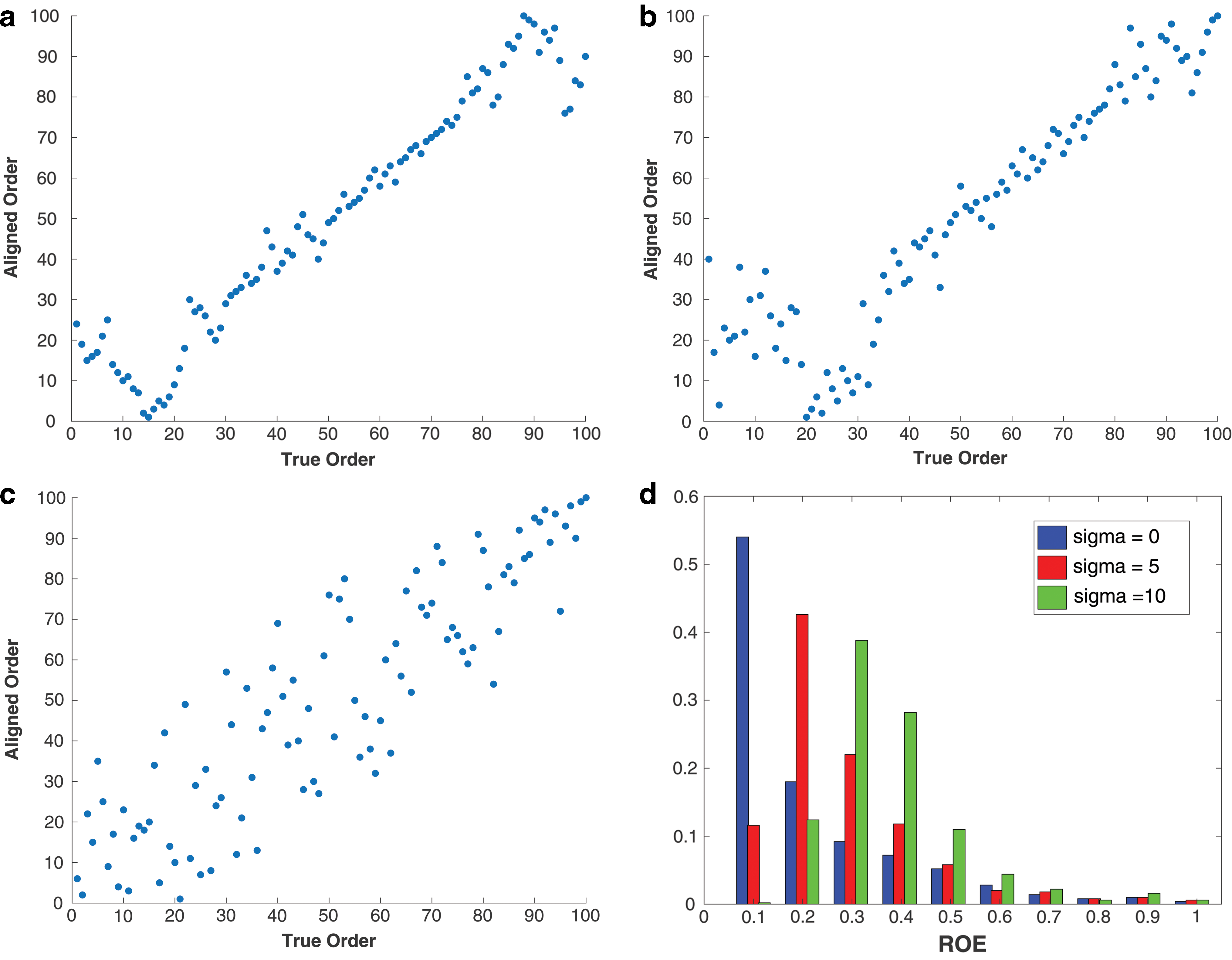
Simulation results with median ROE under different noise levels (σ = 0, 5, 10) are reported in (a), (b), and (c), respectively. The x-axis is the true order of objects; the y-axis is the aligned order of objects. A summary of the simulation is reported in (d). ROE, relative ordering error. Color images are available online.

Path length of the aligned data

In network modeling, a popular approach to study the brain connectivity, ROIs are considered as nodes, and edges between them are established based on their functional connectivity. Many statistics have been proposed to characterize networks, and path length is often used to summarize the efficiency of the network. Recently, the minimum spanning tree (MST) of brain networks has been proposed to summarize the global efficiency of brain function (Olde Dubbelink et al., 2014; Stam et al., 2014; van Dellen et al., 2014). It selects the most efficient and essential path, which connects all the nodes. While this is an appealing way to summarize a network, it fails to detect the differences between the brain connectivity of the normal and demented subjects for the Alzheimer data in the section “Resting-State fMRI Data.” We thus propose a new approach that compares the two groups on a different path, where adjacency of the objects/nodes is determined by the order of the reconfigured brain locations. Specifically, the alignment facilitates an ordered path, ψ(1) → ψ(2) → ψ(3)… → ψ(n − 1) → ψ(n), of the brain connectivity of a subject. We use their ordered path to summarize the efficiency of the brain connectivity, defining a path length: \documentclass{aastex}\usepackage{amsbsy}\usepackage{amsfonts}\usepackage{amssymb}\usepackage{bm}\usepackage{mathrsfs}\usepackage{pifont}\usepackage{stmaryrd}\usepackage{textcomp}\usepackage{portland, xspace}\usepackage{amsmath, amsxtra}\usepackage{upgreek}\pagestyle{empty}\DeclareMathSizes{10}{9}{7}{6}\begin{document} \begin{align*}{L_A} = \mathop \sum \limits_{j = 1}^{n - 1} {{d_{ \psi ( j ) \psi ( j + 1 ) }}}. \tag{4} \end{align*} \end{document}

A traversal distance of a network is usually used to gauge network efficiency. Similar to MST, which is a breadth-first traversal algorithm, path length can be considered as a version of depth-first traversal algorithm, which can be used to measure network efficiency. It is conceivable that an inefficient brain will take longer to travel through, thus it is plausible that path length can capture the deficiency of the brain function of the Alzheimer patients. The data application in the section “Results” underscores the usefulness of this new notion of path length L_A , as it is more effective in detecting the differences between the normal and demented subjects.

A new community detection method

Since the alignment in the section “Alignment of Time Series” arranges similar objects to nearby locations on an interval, one could view these similar objects as a community. An interesting question is how to detect communities by leveraging the reconfiguration after the alignment. The most widely used method to detect communities is to maximize the modularity on networks through thresholded or weighted adjacency matrices. In brain research, these adjacency matrices are usually constructed through functional connectivity maps of ROIs. We proposed a different approach here that takes advantage of the alignment. First, we consider the modularity criterion (Newman, 2006), \documentclass{aastex}\usepackage{amsbsy}\usepackage{amsfonts}\usepackage{amssymb}\usepackage{bm}\usepackage{mathrsfs}\usepackage{pifont}\usepackage{stmaryrd}\usepackage{textcomp}\usepackage{portland, xspace}\usepackage{amsmath, amsxtra}\usepackage{upgreek}\pagestyle{empty}\DeclareMathSizes{10}{9}{7}{6}\begin{document} \begin{align*}{ Q^w } ( { c_1 } , \ldots , { c_n } ) = \frac { 1 } { { { l_w } } } \mathop \sum \limits_ { j , k \in \{ 1 , \cdots , n \} } { \left( { { w_ { jk } } - { \frac { { w_ { j \cdot } } { w_ { k \cdot } } } { { l_w } } } } \right) } \, \times { \rm { } } { { \bf 1 } _ { { \{ c_j } = { c_k \} } } } , \tag { 5 } \end{align*} \end{document}

where w_jk is the weight of the edge between the jth and kth objects; \documentclass{aastex}\usepackage{amsbsy}\usepackage{amsfonts}\usepackage{amssymb}\usepackage{bm}\usepackage{mathrsfs}\usepackage{pifont}\usepackage{stmaryrd}\usepackage{textcomp}\usepackage{portland, xspace}\usepackage{amsmath, amsxtra}\usepackage{upgreek}\pagestyle{empty}\DeclareMathSizes{10}{9}{7}{6}\begin{document}$${w_{j \cdot }} = \sum \nolimits_{k \ne j} {{w_{jk}}}$$ \end{document} ; \documentclass{aastex}\usepackage{amsbsy}\usepackage{amsfonts}\usepackage{amssymb}\usepackage{bm}\usepackage{mathrsfs}\usepackage{pifont}\usepackage{stmaryrd}\usepackage{textcomp}\usepackage{portland, xspace}\usepackage{amsmath, amsxtra}\usepackage{upgreek}\pagestyle{empty}\DeclareMathSizes{10}{9}{7}{6}\begin{document}$${l_w} = \sum \nolimits_{j , k \in \{ 1 , \cdots , n \} } {{w_{jk}}}$$ \end{document} ; and c_j and c_k represent, respectively, the community that the jth and kth objects belong to, where \documentclass{aastex}\usepackage{amsbsy}\usepackage{amsfonts}\usepackage{amssymb}\usepackage{bm}\usepackage{mathrsfs}\usepackage{pifont}\usepackage{stmaryrd}\usepackage{textcomp}\usepackage{portland, xspace}\usepackage{amsmath, amsxtra}\usepackage{upgreek}\pagestyle{empty}\DeclareMathSizes{10}{9}{7}{6}\begin{document}$${1_{ \{ {c_j} = {c_k} \} }}$$ \end{document} is an indicator function indicating whether the jth and kth objects are in the same community. If there are a total of B communities in the network, this formula indicates that the optimization algorithm has to search through Bⁿ possible combinations to find the optimal modularity.

This criterion does not utilize the characteristics of the alignment based on the new reconfiguration proposed above. In the new configuration, one may postulate that objects that are close to each other belong to the same community. With this information, we set out to detect the community structure by locating the boundaries of communities on the new configuration. Since the reconfiguration lies on the 1D space, we formulate the problem as a change-point detection problem. Thus, the modularity criterion is changed to: \documentclass{aastex}\usepackage{amsbsy}\usepackage{amsfonts}\usepackage{amssymb}\usepackage{bm}\usepackage{mathrsfs}\usepackage{pifont}\usepackage{stmaryrd}\usepackage{textcomp}\usepackage{portland, xspace}\usepackage{amsmath, amsxtra}\usepackage{upgreek}\pagestyle{empty}\DeclareMathSizes{10}{9}{7}{6}\begin{document} \begin{align*}{ Q^w } ( B , { b_1 } , \cdots , { b_ { B - 1 } } ) = \frac { 1 }{ { { l_w } } } \mathop \sum \limits_ { j , k \in \ { {\{ 1 , \cdots , n \}} } } { \left( { { w_ { jk } } - { \frac { { w_ { j \cdot } } { w_ { k \cdot } } } { { l_w } } } } \right) } \\ \times \mathop \sum \limits_ { h = 1 } ^B { { 1_ { { { { \{b_ { h- 1 } } \le { { \tilde s } _j } , { { \tilde s } _k } < { b_h \}}}} } } , } \tag { 6 } \end{align*} \end{document}

where (b ₁, ⋯, b_B ₋₁) are the change-points that serve as the boundaries of communities. That is, (b ₁, ⋯, b_B ₋₁) is a subset of \documentclass{aastex}\usepackage{amsbsy}\usepackage{amsfonts}\usepackage{amssymb}\usepackage{bm}\usepackage{mathrsfs}\usepackage{pifont}\usepackage{stmaryrd}\usepackage{textcomp}\usepackage{portland, xspace}\usepackage{amsmath, amsxtra}\usepackage{upgreek}\pagestyle{empty}\DeclareMathSizes{10}{9}{7}{6}\begin{document}$$\{ { \tilde s_2} , \ldots , { \tilde s_n} \}$$ \end{document} , and we further set \documentclass{aastex}\usepackage{amsbsy}\usepackage{amsfonts}\usepackage{amssymb}\usepackage{bm}\usepackage{mathrsfs}\usepackage{pifont}\usepackage{stmaryrd}\usepackage{textcomp}\usepackage{portland, xspace}\usepackage{amsmath, amsxtra}\usepackage{upgreek}\pagestyle{empty}\DeclareMathSizes{10}{9}{7}{6}\begin{document}$${b_0} = { \tilde s_1}$$ \end{document} , b_B = τ. With this set of notations, objects whose aligned positions fall into the interval [b_h _–1, b_h ) are defined as the hth community. This strategy along with the reconfiguration reduces the size of the solution space to 2ⁿ compared with Bⁿ for the modularity in Equation (5). However, there exist two primary challenges for this optimization problem. First, the number of communities B is unknown. Second, to detect the boundaries of communities through optimizing the criteria function, Equation (6) involves a combinatorial optimization problem.

To tackle these challenges, we apply a genetic algorithm (Goldberg et al., 1989) to solve the optimization of the objective function [Eq. (6)]. In a genetic algorithm, candidate solutions are represented by finite-length of strings of alphabets, which are referred to as genes. Each gene is encoded as a binary value 0 or 1, with 1 denoting the boundary of a community. The candidate solutions (b ₁, ⋯, b_B ₋₁) of the criteria function [Eq. (6)] are thus the locations of those genes encoded as 1. More details about the algorithm can be found in a later monograph (Goldberg, 2006).

Results

We apply the methods proposed in the section “Materials and Methods” to resting-state fMRI data from a study of Alzheimer's disease at the University of California, Davis. The study included 172 Alzheimer patients and 67 normal subjects, for whom resting-state fMRI data were obtained for 8 min, resulting in 240 time points of image acquisitions, but the first four observations were discarded to let the scanner magnetization achieve a steady state, so the final length of the BOLD time series was m = 236. The data were preprocessed with SPM8 and subsequently partitioned into 90 cortical regions (based on the AAL system) as described in the section “Resting-State fMRI Data.”

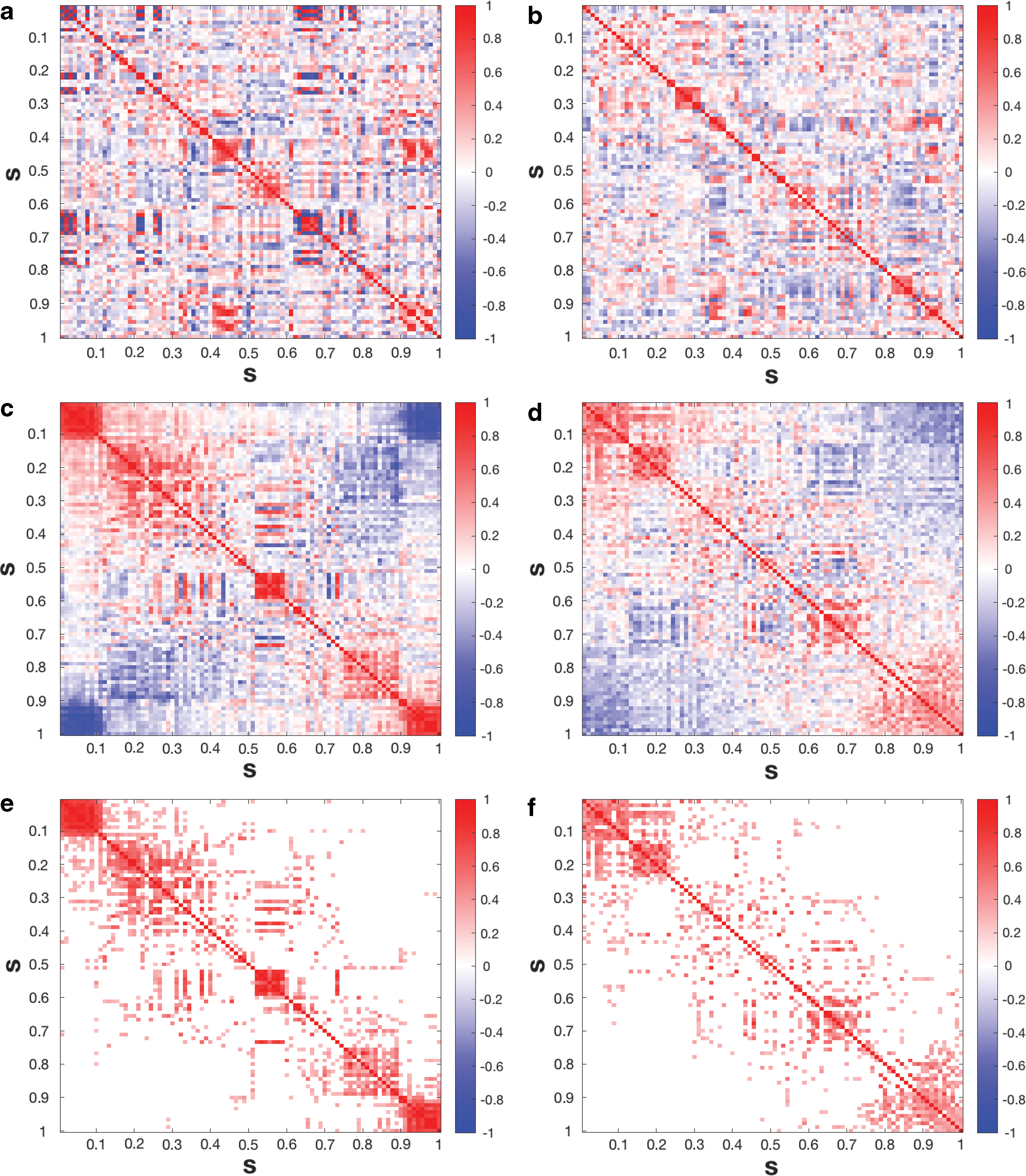
For each subject, this resulted in n = 90 time series, which were subsequently normalized to (X ₁(t),⋯, X ₉₀(t)), where the region locations were arranged in the same order as in the AAL system. The functional connectivity maps of the 90 brain regions are presented in Figure 3a and b for a normal and demented subject, respectively. These subjects are representative of their respective group in the sense that they have the median number of change-points within each group. We then applied the alignment approach to both subjects. The resulting functional connectivity maps based on the reconfiguration are shown in Figure 3c and d. We observe that the information in panels (a) and (b) is difficult to extract, whereas a clearer pattern emerged from each of the panels (c) and (d).

FIG. 3.

Brain image for a representative normal (b and d) and demented (a and c) subject. Panels (a) and (b) show the 90 normalized BOLD signals arranged horizontally according to the AAL ordering, and panels (c) and (d) show the aligned normalized BOLD signals. AAL, automated anatomical labeling; BOLD, blood oxygen level dependent. Color images are available online.

Length of selected path

The path length L_A is computed for each subject, and the average path lengths for the normal and demented groups are 114.69 and 117.47, respectively. The Wilcoxon test reported in Table 1 suggests a marginal significant difference (p = 0.0934 for a two-sided alternative hypothesis) between the two groups and that Alzheimer's disease reduces brain efficiency (shorter path length is more efficient). Here, the Wilcoxon test is used since it does not rely on any parametric assumption and is fairly powerful in comparison with the t-test (Lehmann, 2012). In addition, we apply the MST method (Olde Dubbelink et al., 2014; Stam et al., 2014; van Dellen et al., 2014) to summarize the efficiency of brain network. The average shortest path for the normal and demented groups is 60.37 and 62.29, respectively, but the result is less significant (p = 0.1361 for the Wilcoxon test). This suggests that the new measure L_A is a more effective summary than the MST in existing literature to distinguish normal from demented subjects for brain efficiency.

Table 1.

Test of Network Efficiency

	Network efficiency
	\documentclass{aastex}\usepackage{amsbsy}\usepackage{amsfonts}\usepackage{amssymb}\usepackage{bm}\usepackage{mathrsfs}\usepackage{pifont}\usepackage{stmaryrd}\usepackage{textcomp}\usepackage{portland, xspace}\usepackage{amsmath, amsxtra}\usepackage{upgreek}\pagestyle{empty}\DeclareMathSizes{10}{9}{7}{6}\begin{document}$${{ { \bar {\rm X}}}_1}$$ \end{document}	\documentclass{aastex}\usepackage{amsbsy}\usepackage{amsfonts}\usepackage{amssymb}\usepackage{bm}\usepackage{mathrsfs}\usepackage{pifont}\usepackage{stmaryrd}\usepackage{textcomp}\usepackage{portland, xspace}\usepackage{amsmath, amsxtra}\usepackage{upgreek}\pagestyle{empty}\DeclareMathSizes{10}{9}{7}{6}\begin{document}$${{ \rm{ \bar X}}_2}$$ \end{document}	s₁	s₂	p
Length of MST	60.3687	62.2936	10.0258	8.5955	0.1361
Length of path	114.6889	117.4658	12.9439	10.6568	0.0934

Normal group is indexed by 1 and demented group by 2.

The p-values are calculated from the Wilcoxon rank-sum test.

MST, minimum spanning tree.

Community detection

In addition to using the selected path length to measure the efficiency of brain function, we are also interested in exploring another important topological property of brain networks, the community structure in terms of modularity. A modular organization characterizes many important biological systems, including brain networks. The modularity is considered as a topological structure that can combine advantages of high clustering and high efficiency and optimize between the brain wiring cost and efficiency (Bullmore and Sporns, 2012). This concept is then utilized to detect community structures by maximizing Q as commonly performed (Newman, 2006). Given the new configuration obtained through the proposed alignment method and based on the discussion in the section “A New Community Detection Method,” we adopted the modified Q in Equation (6) to detect the community structure. This modularity is used to measure how well the defined communities maximize the within-group connection and minimize the between-group connection.

Inspired by the framework of exponential random graph modeling (Simpson et al., 2011; Van Wijk et al., 2010), we apply a transformation w_jk = exp(ρ_jk ) to transfer the cosine angle into a nonnegative weight. We applied the change-point analysis in the section “A New Community Detection Method” to each subject and observed block diagonal structures for both the normal and demented subjects in Figures 4c and d. Furthermore, we applied a threshold \documentclass{aastex}\usepackage{amsbsy}\usepackage{amsfonts}\usepackage{amssymb}\usepackage{bm}\usepackage{mathrsfs}\usepackage{pifont}\usepackage{stmaryrd}\usepackage{textcomp}\usepackage{portland, xspace}\usepackage{amsmath, amsxtra}\usepackage{upgreek}\pagestyle{empty}\DeclareMathSizes{10}{9}{7}{6}\begin{document}$${{\bf 1}_{ \left[ {0.25 , 1} \right] }} ( { \rho _{jk}} )$$ \end{document} (Buckner et al., 2009) to aid the visualization of the modularity structure. After thresholding the correlation matrix (Fig. 4e, f), we observed block structures appearing along the diagonal of correlation matrix and that the correlation between these blocks is sparse. This is consistent with the characteristic of modular structures where members within the same community connect densely and members between communities connect sparsely.

FIG. 4.

Brain image for a representative normal (b, d, and f) and demented (a, c, and e) subject. Panels (a) and (b) show the correlation of 90 normalized BOLD signals arranged according to the AAL ordering, and panels (c) and (d) show the correlations of the aligned normalized BOLD signals. Panels (e) and (f) show the thresholded (>0.25) correlations for the aligned normalized BOLD signals. Color images are available online.

We also compared our approach with the algorithm from the brain connectivity toolbox [BCT; Rubinov and Sporns (2010)] on all subjects. The results shown in Figure 5a are based on our proposed algorithm and the Louvain Method for community detection and confirm that the communities detected by our approach are as good as those by BCT. In conclusion, these results indicate that our community detection approach conveys valuable information.

FIG. 5.

(a) Box plots of modularity comparing BCT (Rubinov and Sporns, 2010) with our approach. (b) Box plots of number of communities comparing BCT with our approach. BCT, brain connectivity toolbox. Color images are available online.

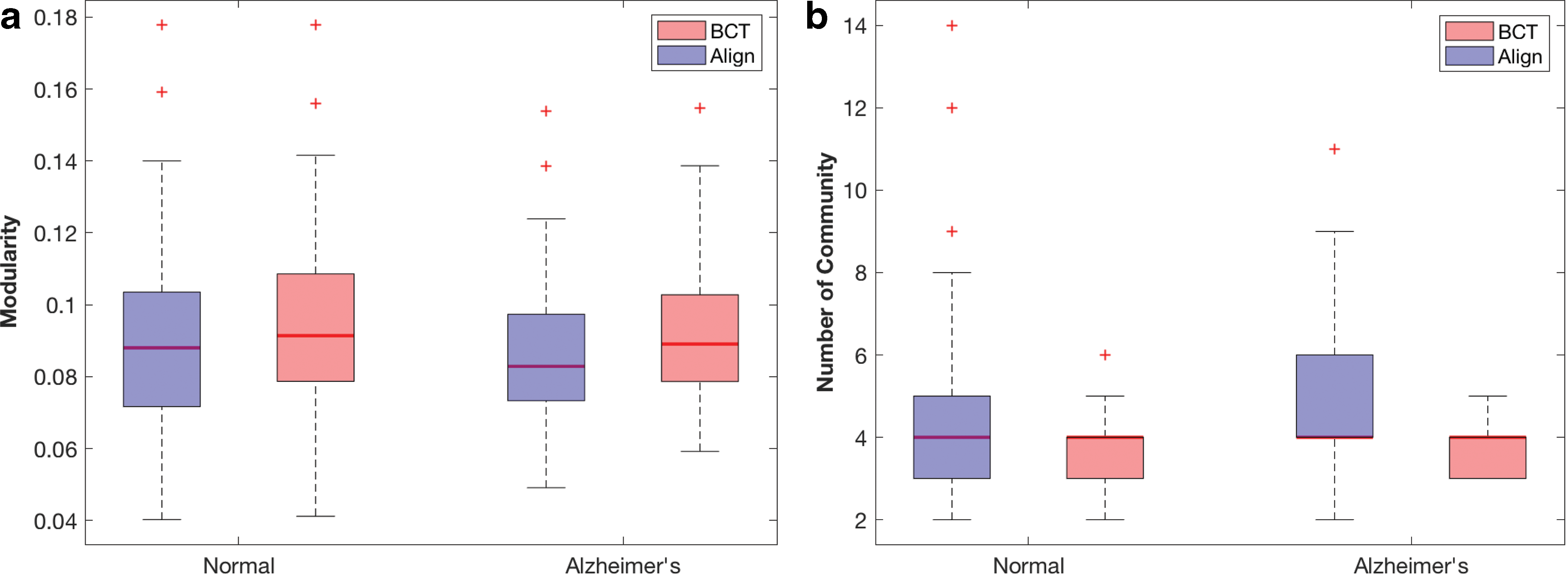
Finally, we compared modularities and numbers of communities between the normal and demented subjects. The average modularity, as shown in Table 2, is 0.0896 and 0.0849 for the normal and demented groups, respectively. Although not statistically significant, our method led to a smaller p-value (p = 0.1210) than the one from BCT (p = 0.1539), suggesting that the demented group seems to have less efficient community structures.

Table 2.

Test of Modularity

	Rank-sum test: modularity
	\documentclass{aastex}\usepackage{amsbsy}\usepackage{amsfonts}\usepackage{amssymb}\usepackage{bm}\usepackage{mathrsfs}\usepackage{pifont}\usepackage{stmaryrd}\usepackage{textcomp}\usepackage{portland, xspace}\usepackage{amsmath, amsxtra}\usepackage{upgreek}\pagestyle{empty}\DeclareMathSizes{10}{9}{7}{6}\begin{document}$${{ \rm{ \bar X}}_1}$$ \end{document}	\documentclass{aastex}\usepackage{amsbsy}\usepackage{amsfonts}\usepackage{amssymb}\usepackage{bm}\usepackage{mathrsfs}\usepackage{pifont}\usepackage{stmaryrd}\usepackage{textcomp}\usepackage{portland, xspace}\usepackage{amsmath, amsxtra}\usepackage{upgreek}\pagestyle{empty}\DeclareMathSizes{10}{9}{7}{6}\begin{document}$${{ \rm{ \bar X}}_2}$$ \end{document}	s₁	s₂	p
Align	0.0896	0.0849	0.0217	0.0194	0.1210
BCT	0.0949	0.0906	0.0205	0.0181	0.1539

Normal group is indexed by 1 and demented group by 2.

The p-values are calculated from the Wilcoxon rank-sum test.

BCT, brain connectivity toolbox.

The average number of communities, as shown in Table 3, is 4.2500 and 4.8955 for the normal and demented groups, respectively. Our method shows that the two groups differ significantly (p = 0.0032) in terms of the number of communities with the demented group split into more communities. But BCT is less effective to detect this difference (p = 0.0625). Combining the results in Tables 2 and 3 and Figure 5 with the findings on the path length, we conclude that in comparison to the normal subjects, the demented subjects not only have less global efficiency but also have less intact local functional modules.

Table 3.

Test of the Number of Communities

	Rank-sum test: number of communities
	\documentclass{aastex}\usepackage{amsbsy}\usepackage{amsfonts}\usepackage{amssymb}\usepackage{bm}\usepackage{mathrsfs}\usepackage{pifont}\usepackage{stmaryrd}\usepackage{textcomp}\usepackage{portland, xspace}\usepackage{amsmath, amsxtra}\usepackage{upgreek}\pagestyle{empty}\DeclareMathSizes{10}{9}{7}{6}\begin{document}$${{ \bar{ \rm {X}}}_1}$$ \end{document}	\documentclass{aastex}\usepackage{amsbsy}\usepackage{amsfonts}\usepackage{amssymb}\usepackage{bm}\usepackage{mathrsfs}\usepackage{pifont}\usepackage{stmaryrd}\usepackage{textcomp}\usepackage{portland, xspace}\usepackage{amsmath, amsxtra}\usepackage{upgreek}\pagestyle{empty}\DeclareMathSizes{10}{9}{7}{6}\begin{document}$${{ \rm{ \bar X}}_2}$$ \end{document}	s₁	s₂	p
Align	4.2500	4.8955	1.7576	1.9473	0.0032
BCT	3.8198	4.0149	0.7391	0.7281	0.0625

Normal group is indexed by 1 and demented group by 2.

The p-values are calculated from the Wilcoxon rank-sum test.

Discussion and Conclusion

We propose a new approach to visualize neuroimaging data using BOLD signals as the platform. The proposed approach compresses the 3D spatial locations of the brain regions into spatial locations of a 1D space, so that the temporal signals of fMRI time series can be aligned along a horizontal axis and the heat map (Fig. 3) can be used to visualize the aligned objects. In addition to visualization, two new approaches emerged from the alignment idea. The first is a new summary for the global efficiency of the functional connectivity of an individual brain. This new summary is based on the path length along the aligned brain location and is shown in the section “Results” to be effective in distinguishing Alzheimer's and normal subjects, thereby providing new insights in how Alzheimer's disease alters the structure of brain connectivity.

The second by-product is a new method to detect communities through change-points locations of the functional connectivity as brain regions between two change-points are more similarly connected than those across change-points. Thus, instead of examining a 90 × 90 adjacency matrix, the alignment reduces the adjacency matrix to diagonal subblocks of sizes n ₁, …, n_B . Such a data reduction is feasible because we have reconfigured the objects by aligning them. When using the weighted modularity criteria, our community detection method performs competitively with the BCT approach.

In summary, the alignment approach opens a new way to explore complex spatially index objects. While we illustrate our approach with time series objects, the proposed method is applicable to any functions or abstract objects. As we have only performed the alignment at the subject level, an interesting question is whether it makes sense to do a unified alignment for a group of subjects, that is, whether it is reasonable to use the same ordering for all subjects in a group. The answer is likely to depend on the homogeneity of the group. One major advantage of the alignment method is that it alleviates or overcomes the curse of high dimensionality for object data. For instance, by aligning the BOLD signal of a subject, we provide an ordering for spatially index signals, so the realigned BOLD signals could be viewed as longitudinal functional data (Chen and Müller, 2012) or smooth 2D functional data.

Since methods to deal with such functional data are plentiful due to the fast growing interest in functional data analysis (Ramsay and Silverman, 2007; Wang et al., 2016), the alignment approach proposed in this article bridges a gap between the analysis for high-dimensional object data and smooth object data. There is clearly a vast array of methods one can borrow from the statistical literature of functional data analysis once the alignment has been completed, including functional principle component analysis, classification, clustering, and prediction. This could be an interesting future direction to explore.

Footnotes

Acknowledgment

The research of J.-L.W. is supported by NSF grant DMS-15-12975 and NIH Grants 7UG3OD023313 and 1UH3OD023313.

Author Disclosure Statement

No competing financial interests exist.

References

Bandettini

, Jesmanowicz

, Wong

, Hyde

. 1993. Processing strategies for time-course data sets in functional MRI of the human brain. Magn Reson Med, 30:161–173.

Biswal

, Yetkin

, Haughton

, Hyde

. 1995. Functional connectivity in the motor cortex of resting human brain using echo-planar MRI. Magn Reson Med, 34:537–541.

Borg

, Groenen

. 2005. Modern Multidimensional Scaling: Theory and Applications. New York, NY: Springer Science & Business Media.

Buckner

, Sepulcre

, Talukdar

, Krienen

, Liu

, Hedden

, et al. 2009. Cortical hubs revealed by intrinsic functional connectivity: mapping, assessment of stability, and relation to Alzheimer's disease. J Neurosci, 29:1860–1873.

Bullmore

, Sporns

. 2012. The economy of brain network organization. Nat Rev Neurosci, 13:336–349.

Castruccio

, Ombao

, Genton

. 2018. A scalable multi-resolution spatio-temporal model for brain activation and connectivity in fMRI data. Biometrics, 74:823–833.

Chen

, Chen

, Müller

H-G

, Wang

J-L

. 2011. Stringing high-dimensional data for functional analysis. J Am Stat Assoc, 106:275–284.

Chen

, Müller

H-G

. 2012. Modeling repeated functional observations. J Am Stat Assoc, 107:1599–1609.

Cordes

, Haughton

, Arfanakis

, Carew

, Turski

, Moritz

, et al. 2001. Frequencies contributing to functional connectivity in the cerebral cortex in “resting-state” data. Am J Neuroradiol, 22:1326–1333.

10.

De Leeuw

. 1977. Applications of convex analysis to multidimensional scaling. In Barra

, Brodeau

, Romier

, van Cutsem

(eds.) Recent Developments in Statistics. Amsterdam, The Netherlands: North-Holland; pp. 133–145.

11.

Ferreira

, Zhao

. 2016. Time series clustering via community detection in networks. Inf Sci, 326:227–242.

12.

Friston

. 2011. Functional and effective connectivity: a review. Brain Connect, 1:13–36.

13.

Friston

, Frith

, Fletcher

, Liddle

, Frackowiak

RSJ

. 1996. Functional topography: multidimensional scaling and functional connectivity in the brain. Cereb Cortex, 6:156–164.

14.

Friston

, Frith

, Liddle

, Frackowiak

RSJ

. 1993. Functional connectivity: the principal-component analysis of large (pet) data sets. J Cereb Blood Flow Metab, 13:5–14.

15.

Goldberg

, Deb

, Korb

. 1989. Messy genetic algorithms: motivation, analysis, and first results. Complex Syst. 493–530.

16.

Goldberg

. 2006. Genetic Algorithms. Chennai: Pearson Education India.

17.

Granger

, Newbold

. 1974. Spurious regressions in econometrics. J Econometrics, 2:111–120.

18.

Greicius

, Krasnow

, Reiss

, Menon

. 2003. ‘Functional connectivity in the resting brain: a network analysis of the default mode hypothesis’, Proc Natl Acad Sci, 100:253–258.

19.

Hampson

, Peterson

, Skudlarski

, Gatenby

, Gore

. 2002. Detection of functional connectivity using temporal correlations in MR images. Hum Brain Mapp, 15:247–262.

20.

Hollander

, Wolfe

, Chicken

. 2013. Nonparametric Statistical Methods, Vol. 751. Hoboken, NJ: John Wiley & Sons.

21.

Horwitz

. 2003. The elusive concept of brain connectivity. Neuroimage, 19:466–470.

22.

Hsing

, Eubank

. 2015. Theoretical Foundations of Functional Data Analysis, with an Introduction to Linear Operators. West Sussex, UK: John Wiley & Sons.

23.

Kendall

. 1938. A new measure of rank correlation. Biometrika, 30:81–93.

24.

Kendall

. 1962. Rank Correlation Methods. London: Charles Griffin and Company.

25.

Lehmann

. 2012. Parametric versus nonparametrics: two alternative methodologies. In: Rojo

(ed.) Selected Works of EL Lehmann. Boston, MA: Springer; pp. 437–445.

26.

Newman

MEJ

. 2006. Modularity and community structure in networks. Proc Natl Acad Sci, 103:8577–8582.

27.

Olde Dubbelink

, Hillebrand

, Stoffers

, Deijen

, Twisk

, Stam

, Berendse

. 2014. Disrupted brain network topology in parkinson's disease: a longitudinal magnetoencephalography study. Brain, 137:197–207.

28.

Park

, Aston

, Ferraty

. 2016. Stable and predictive functional domain selection with application to brain images. arXiv preprint arXiv:1606.02186.

29.

Preti

, Bolton

, Van De Ville

. 2017. The dynamic functional connectome: state-of-the-art and perspectives. Neuroimage, 160, 41–54.

30.

Ramsay

, Silverman

. 2007. Applied Functional Data Analysis: Methods and Case Studies. New York, NY: Springer-Verlag.

31.

Rubinov

, Sporns

. 2010. Complex network measures of brain connectivity: uses and interpretations. Neuroimage, 52:059–1069..

32.

Shinkareva

, Ombao

, Sutton

, Mohanty

, Miller

. 2006. Classification of functional brain images with a spatio-temporal dissimilarity map. Neuroimage, 33:63–71.

33.

Simpson

, Hayasaka

, Laurienti

. 2011. Exponential random graph modeling for complex brain networks. PLoS One, 6:e20039.

34.

Spearman

. 1904. The proof and measurement of association between two things. Am J Psychol, 15:72–101.

35.

Sporns

. 2010. Networks of the Brain. Cambridge, MA: MIT Press.

36.

Stam

, Tewarie

, Dellen

, van Straaten

, Hillebrand

, Mieghem

. 2014. The trees and the forest: characterization of complex brain networks with minimum spanning trees. Int J Psychophysiol, 92:129–138.

37.

van Dellen

, Douw

, Hillebrand

, de Witt Hamer

, Baayen

, Heimans

, et al. 2014. Epilepsy surgery outcome and functional network alterations in longitudinal MEG: a minimum spanning tree analysis. Neuroimage, 86:354–363.

38.

Van Den Heuvel

, Pol

HEH

. 2010. Exploring the brain network: a review on resting-state fmri functional connectivity. Eur Neuropsychopharmacol, 20:519–534.

39.

Van Wijk

, Stam

, Daffertshofer

. 2010. Comparing brain networks of different size and connectivity density using graph theory. PLoS One, 5:e13701.

40.

Wang

J-L

, Chiou

J-M

, Müller

H-G

. 2016. Functional data analysis. Annu Rev Stat Appl, 3:257–295.

41.

Welchew

, Honey

, Sharma

, Robbins

, Bullmore

. 2002. Multidimensional scaling of integrated neurocognitive function and schizophrenia as a disconnexion disorder. Neuroimage, 17:1227–1239.

42.

Welchew

, Ashwin

, Berkouk

, Salvador

, Suckling

, Baron-Cohen

, Bullmore

. 2005. Functional disconnectivity of the medial temporal lobe in asperger's syndrome. Biol Psychiatry, 57:991–998.

43.

Zang

, Jiang

, Lu

, He

, Tian

. 2004. Regional homogeneity approach to fMRI data analysis. Neuroimage, 22:394–400.