New Graph-Theoretical-Multimodal Approach Using Temporal and Structural Correlations Reveals Disruption in the Thalamo-Cortical Network in Patients with Schizophrenia

Abstract

Schizophrenia has been understood as a network disease with altered functional and structural connectivity in multiple brain networks compatible to the extremely broad spectrum of psychopathological, cognitive, and behavioral symptoms in this disorder. When building brain networks, functional and structural networks are typically modeled independently: Functional network models are based on temporal correlations among brain regions, whereas structural network models are based on anatomical characteristics. Combining both features may give rise to more realistic and reliable models of brain networks. In this study, we applied a new flexible graph-theoretical-multimodal model called FD (F, the functional connectivity matrix, and D, the structural matrix) to construct brain networks combining functional, structural, and topological information of magnetic resonance imaging (MRI) measurements (structural and resting-state imaging) to patients with schizophrenia (n = 35) and matched healthy individuals (n = 41). As a reference condition, the traditional pure functional connectivity (pFC) analysis was carried out. By using the FD model, we found disrupted connectivity in the thalamo-cortical network in schizophrenic patients, whereas the pFC model failed to extract group differences after multiple comparison correction. We interpret this observation as evidence that the FD model is superior to conventional connectivity analysis, by stressing relevant features of the whole-brain connectivity, including functional, structural, and topological signatures. The FD model can be used in future research to model subtle alterations of functional and structural connectivity, resulting in pronounced clinical syndromes and major psychiatric disorders. Lastly, FD is not limited to the analysis of resting-state functional MRI, and it can be applied to electro-encephalography, magneto-encephalography, etc.

Introduction

Schizophrenia is a mental illness with heterogeneous symptoms, including positive symptoms such as delusions and hallucinations and negative symptoms such as reduced emotional expression, lack of motivation, among others. It has been hypothesized that schizophrenia could be understood as a network disease with dysfunctional connectivity between multiple brain regions (Andreasen et al., 1998; Friston, 1999; Friston and Frith, 1995). According to this hypothesis, symptoms are assumed to emerge from a failure in the functional integration of information processing in the brain (Garrity et al., 2007). Several studies have found abnormal functional and structural connectivity in multiple brain networks, supporting the theory of schizophrenia as a dysconnectivity syndrome (Friston and Frith, 1995; Hadley et al., 2016) and suggesting functional and structural disturbances in whole-brain connectivity (Andreasen and Pierson, 2008; Barch, 2014; Cocchi et al., 2014; Kühn et al., 2012; Nelson et al., 1998; Singh et al., 2015; van den Heuvel and Fornito, 2014; Zalesky et al., 2012). Moreover, overlapping of disruption in both these functional and structural modalities has been suggested (Liu et al., 2019; Nelson et al., 2017), as well as synchronous changes of fusion measures of brain anatomy and brain networks from independent component analyses (Calhoun and Sui, 2016; Qi et al., 2019) and dynamic functional connectivity networks (Abrol et al., 2017).

Brain networks in neuroimaging using functional magnetic resonance imaging (fMRI) are composed by brain areas, called nodes, and the connections between nodes are called links (van den Heuvel and Hulshoff Pol, 2010). Links in the brain networks can be constructed by using structural or functional information. In structural networks, links are built by using correlations of morphometric features from diffusion tensor imaging (DTI) and MRI as fibers in the white matter (WM)/total number of interconnecting streamlines, cortical thickness or gray matter (GM) volume. However, in functional networks, two regions are said to be functionally connected, and therefore, engaged in information processing, if they present a temporal correlation. Links constructed using these temporal correlations are usually calculated by using Pearson's correlation coefficient.

Typically, structural and functional brain networks are calculated and analyzed separately, for example, functional networks are built by using solely temporal correlations given by Pearson correlation function, regardless of any structural information. However, combining these two equally important features of brain function and morphology might give rise to more realistic, complete, and even reliable models of brain networks as existing interactions between structural and functional connectivity (Abrol et al., 2017; Battiston et al., 2017; Bowman et al., 2012; Calamante et al., 2017; Calhoun and Sui, 2016; Chu et al., 2018; Kang et al., 2017; Xue et al., 2015). Focusing on schizophrenia, recent effort has been made to combine different brain imaging modalities and analysis, in both resting state (Abrol et al., 2017; Liu et al., 2019; Nelson et al., 2017; Qi et al., 2019; Sui et al., 2015; Wang et al., 2015) and task (Calhoun et al., 2006; García-Martí et al., 2012), being able to successfully identify group differences in relevant brain areas for schizophrenia. In addition, concatenation of functional connectivity and anatomical features used in classification of schizophrenia (Qureshi et al., 2017), interestingly, provided the highest predictive accuracy (Guo et al., 2018).

In this framework, a new graph-theoretical-multimodal model was proposed to study connectivity, and this is called the FD model (F, the functional connectivity matrix, and D, the structural matrix) (Finotelli and Dulio, 2015). The FD model adds, to the pure functional connectivity (pFC), structural and topological information that can be obtained from multiple different techniques: topological information given by nodal degree, functional connectivity matrix given by Pearson's correlation, Spearman correlation, mutual information, Granger causality or any other correlation/causality index, and for the structural matrix D, from morphometric characteristics, such as volume, cortical thickness and GM/WM connectivity, as well as the Euclidean distances between pairs of brain areas, DTI data, etc. The FD model has been successfully applied to electro-encephalography (EEG) data, with subjects performing a musical task (Finotelli et al., 2016), and to synthetic data simulation of the human's brain functional activity at rest (Dulio et al., 2018).

The aim of this article is to analyze whole-brain network of patients with schizophrenia and a matched group of healthy individuals by means of two different models. First, the pFC model, commonly used in the literature, takes only the functional connectivity into consideration. Second, the FD model utilizes not only the functional data but also structural and topological properties of the cerebral network.

Methods

Participants

Forty-one were healthy individuals, and 35 individuals who met the criteria for a diagnosis of schizophrenia following the International Classification for Diseases and Related Health Problems (ICD-10) were included in the study. The recruitment of patients diagnosed with schizophrenia took place at St. Hedwig Hospital, Department for Psychiatry and Psychotherapy of the Charité-Universitätsmedizin Berlin (Germany). A trained clinician assessed the severity of symptoms with the Scale for Assessment of Negative Symptoms (Andreasen, 1989), and the Scale for Assessment of Positive Symptoms (Andreasen, 1984). For the healthy individuals, the recruitment was accomplished by using advertisements and flyers. Healthy individuals did not meet the criteria for any psychiatric disorder based on information acquired with the Mini International Neuropsychiatric Interview (Ackenheil et al., 1999) and were not in current or past psychotherapy of an ongoing mental health-related problem. Healthy individuals matched the group of patients in terms of age, sex, handedness, and level of education (Table 1). Handedness was acquired by using the Edinburgh Handedness Inventory, cognitive functioning was tested by using the Brief Assessment of Cognition in Schizophrenia (Keefe et al., 2008), and verbal intelligence was assessed with a German Vocabulary Test (Schmidt and Metzler, 1992). All procedures of the study were approved by the ethics committee of the Charité-Universitätsmedizin Berlin.

Table 1.

Demographics and Clinical Characteristics

	HC (n = 41)	SCZ (n = 35)	p-Value
	Mean (standard deviation)	Mean (standard deviation)	p-Value
Gender (male/female)	24/17	21/14
Age (years)	35.2 (11.0)	35.3 (10.8)	0.953
Framewise displacement	0.15 (0.02)	0.17 (0.02)	0.42
Edinburg Handedness Inventory^a	79.4 (38.5)	75.56 (52.6)	0.742
Education (years)	14.1 (2.9)	13.1 (3.8)	0.183
BACS^a	270.4 (37.0)	234.1 (28.4)	<0.001
Verbal intelligence (IQ)^a	100.5 (10.6)	94.4 (12.8)	0.031
Illness duration (years)		9.4 (8.8)
Illness onset (age in years)		25.6 (8.9)
Chlorpromazine-equivalent (mg)		317.1 (221.6)
SANS composite score^a		20.2 (12.0)
SAPS composite score^a		15.4 (14.9)

Sum score of items reported.

BACS, Brief Assessment of Cognition in Schizophrenia; HC, healthy control; SANS, Scale for Assessment of Negative Symptoms; SAPS, Scale for Assessment of Positive Symptoms; SCZ, schizophrenia.

MRI data acquisition

Images were collected on a Siemens Tim Trio 3T scanner (Erlangen, Germany) with a 12-channel head coil. Structural images were obtained by using a T1-weighted magnetization-prepared gradient-echo sequence (MP-RAGE) based on the Alzheimer's Disease Neuroimaging Initiative (ADNI) protocol (repetition time [TR] = 2500 msec; echo time [TE] = 4.77 msec; inversion time (TI) = 1100 msec, acquisition matrix = 256 × 256 × 176; flip angle = 7°; 1 × 1 × 1 mm³ voxel size). Whole-brain functional resting-state images during 5 min were collected by using a T2*-weighted echo-planar imaging sequence sensitive to blood-oxygen-level dependent (BOLD) contrast (TR = 2000 msec, TE = 30 msec, image matrix = 64 × 64, field of view [FOV] = 216 mm, flip angle = 80°, slice thickness = 3.0 mm, distance factor = 20%, voxel size 3 × 3 × 3 mm³, 36 axial slices). Before resting-state data acquisition was started, participants were in the scanner for about 10 min, during which a localizer and the anatomical images were acquired so that subjects could get used to the scanner noise. During resting-state data acquisition, participants were asked to close their eyes and relax during data acquisition. Exclusion criteria were brain abnormalities and excess movement in the scanner.

Preprocessing of resting-state data

The first five images were discarded to ensure for steady-state longitudinal magnetization. The data were then corrected for slice timing and realigned. Individual T1 images were coregistered to functional images and segmented into GM, WM, and cerebrospinal fluid. Data were spatially normalized to the MNI template and, to improve signal-to-noise ratio, spatially smoothed with a 6-mm FWHM. Motion and signals from WM and cerebrospinal fluid were regressed. Data were then filtered (0.01–1 Hz) to reduce physiological high-frequency respiratory and cardiac noise and low-frequency drift and, finally, detrended. All steps of data preprocessing were done by using SPM12, except filtering that was applied by using the REST toolbox (Song et al., 2011). In addition, to control for motion, the voxel-specific mean framewise displacement was calculated (Power et al., 2012). Framewise displacement values were below the default threshold of 0.5 for control and patient group (Table 1).

Voxel-based morphometry

Voxel-based morphometry (VBM), an unbiased objective technique, has been developed to investigate regional differences in the brain anatomy (Mechelli et al., 2005) by using MRI. VBM estimates regional WM and/or GM volume. Structural data were processed by means of the VBM8 toolbox and SPM8 with default parameters. The VBM8 toolbox involves bias correction, tissue classification, and affine registration. The affine registered GM and WM segmentations were used to build a customized DARTEL diffeomorphic anatomical registration through an exponentiated lie algebra template. Then, warped GM and WM segments were created. Modulation was applied to preserve the volume of a particular tissue within a voxel by multiplying voxel values in the segmented images by the Jacobian determinants derived from the spatial normalization step. In effect, the analysis of modulated data tests for regional differences in the absolute amount (volume) of GM.

The mathematical models

In this section, we introduce the two models involved in this study: pFC and FD, and we describe the basic concepts of Graph Theory and Linear Algebra (the matrices).

Network representation: Adjacency matrix is the mathematical expression of a network. In brain networks, each row and column is a neural element and how they are related are the weights. If the weights are obtained by calculating the pFC between n neural elements, for example, voxels or brain regions, the resulting adjacency matrix will have n rows and n columns, being called a square matrix. Importantly, by exchanging the rows with the columns in a matrix A returns a matrix A^T called the transpose of A. A^T is so characterized by having n rows and n columns. If A = A^T , the matrix is said to be symmetric, which holds to pFC but not to effective connectivity due to the different nature of the measure.

Degree of a node: The degree of a neural element (or node) is the sum of all its connections in the network. This topological metric is useful to get information about the centrality of the node in the network and a first step in understanding whether the node can take on the role of a hub. Hubs play a central role in the network, integrating and distributing information in very effective ways due to the number and positioning of their connections in a network.

Formally, a graph G refers to a set of vertices (or nodes) and of edges (or links) that connect the vertices. Two nodes are said to be adjacent if they are end-points of an edge. An important number associated with each vertex is its degree. The degree of an arbitrary node v is the number deg(v) of the adjacent nodes. In our study, the nodes represent the cerebral areas in the automated anatomical labeling (AAL) template. Importantly, a graph G can be equivalently represented by a square matrix A_G . This is done by defining a weight for each edge of the graph G. For each i ∈{1, 2,…,m} and j ∈{1, 2,…,n}, the entry (ij) of the matrix A_G is the weight of the edge connecting the nodes i and j, if it exists, or 0 otherwise.

The degree of the nodes can be calculated by adding all the nonzero elements of the columns (or equivalently, due to the symmetry, of the rows) of the connectivity matrix associated to that node.

The pFC model: Functional connectivity computed based on Pearson correlation coefficients is the most frequently applied method in the literature. This is a measure of linear correlation between two variables X and Y. The correlation values range from −1 to +1. When applied to neuroimaging, the correlations refer to a statistical dependence between physiological recordings that have been acquired from distinct neural elements (nodes). In fMRI, the neural elements are most likely brain regions or voxels and the physiological recordings are the indirect measure of the neural activity: The BOLD. The Pearson correlation coefficient is symmetric, that is, the correlation between X and Y is the same as the correlation between Y and X: corr(X,Y) = corr(Y,X). This leads to an important property for the mathematical description of a network: The adjacency matrix is symmetric.

The FD model: The FD model combines functional information given by the pFC matrix with structural and topological information; this model computes the connectivity not only as a function of the strength of the statistical correlations as in pFC but also as a function of the node degrees and the structural connectivity (for details, see Finotelli and Dulio, 2015; Finotelli et al., 2018).

In the FD model, the general formula for calculating the functional weight of an arbitrary entry w_ij of the matrix W is: $w_{i j} = \frac{d e g (i) d e g (j)}{W_{m a x} (t)} e^{- (d_{i j} - {f_{i j}}^{s})}$ (1)

where deg is the degree calculated as explained earlier; d_ij and f_ij ^s are, respectively, the generic entry of position (ij) in the matrix D, which incorporates the structural information of the brain network, and in the matrix F^s , the functional connectivity matrix F, whose entries represent the positive statistical dependence between the time series of measured neurophysiological signals. Note that depending on the purpose of a particular study, F^s can be also thresholded (Finotelli et al., 2016).

The generic entry of W, w_ij, is within the range of 0 and +1, and therefore comparable to pFC. The exponent is the difference of two matrices, F^s and D, that should be characterized by having their entries in (nearly) the same range of variability. The FD model can employ both structural and functional data obtained from multiple different techniques. For more details regarding the explicit structure of Equation (1), we refer the reader to Finotelli and Dulio (2015). The only precaution is that D should be normalized to be comparable to matrix F^s .

In summary, the matrix generation of the FD model is obtained by means of functional data (embedded in matrix F) and structural information (embedded in matrix D). We would like to point out that the cerebral areas considered for both matrices generation are the same. In other words, the number of nodes and their labels considered in this work always match in both F and D. Moreover, the value of each of the entries of D, when necessary, as in the case of physical distances between pairs of cerebral areas, is normalized in the range [0, 1].

In this study, we constructed the functional connectivity matrices F^s using positive values from Pearson's correlation, the most popular connectivity measure, and the structural connectivity matrix D using VBM estimates of regional GM volume, resulting in a structural connectivity pattern matrix (He et al., 2007). VBM is a function of cortical thickness and cortical area, and therefore an important unbiased morphometry measure.

Connectivity matrices

Functional connectivity matrix generation: For each subject, the time series of each brain area (node) segmented according to the AAL 90 atlas (Tzourio-Mazoyer et al., 2002) were extracted by using the REST toolbox (Song et al., 2011). Then, the linear correlation between all pair of nodes (i,j = 1,…,90) was calculated by using Pearson's correlation coefficient, resulting in a matrix F = [f_ij]. Two nodes were considered connected, and therefore a link set to f_ij, if the Pearson's correlation coefficient was statistically significant. Due to the FD model, negative and self-correlations were not considered: Negative f_ij was set to 0 as well as all the elements on the principal diagonal of the matrices. This process originates from the matrix F^s = [f_ij ^s]. Please note that the pFC is composed only by the F matrices, whereas the FD model follows Equation (1).

Inferred structural connectivity matrix generation: VBM was calculated as explained earlier. We inferred the structural matrix based on the covariation of GM volume as calculated for the functional connectivity matrix: Regions were segmented into the same AAL 90 regions as mentioned earlier. Two regions (nodes i,j = 1,…,90) were assumed to be connected if the correlation of regional GM across subjects d_ij given by Pearson's correlation coefficient was statistically significant, resulting in a structural connectivity pattern matrix D = [d_ij] for each group (He et al., 2007). Likewise, we did not consider negative and self-correlations due to the FD model: Negative d_ij was set to 0 as well as all the elements on the principal diagonal of the matrices. The inferred structural connectivity matrix is an indirect measure of the anatomical connectivity. This approach was chosen due its simplicity, technical easiness (T1 images) and to the fact that there is evidence of a strong correlation between axonally connected brain regions and cortical thickness (Bassett et al., 2008; Lerch et al., 2006).

The FD model: W matrix generation: For each subject, the entries w_ij (i,j = 1,…,90) of the FD model matrices W were calculated by using Equation (1), where deg(i) and deg(j) are the degree of nodes i and j, respectively; D = [d_ij], is the structural matrix; and F^s = [f_ij ^s] is the matrix obtained as explained earlier. For every matrix W, the normalization procedure is performed by dividing all the entries of W, w_ij, by W_max, the maximum value of W [for details, see Finotelli and Dulio (2015) and Finotelli et al. (2016)].

Statistical analysis

In both pFC and FD models, we performed a permutation-based unpaired t-test to compare the control and the patient group. We tested the null hypothesis of equality between the distributions of patients and controls on link î-ĵ against the alternative of difference in distribution between the two groups on the same link in both pFC and FD models. The test was based on the computation of the squared t-test statistic over all possible permutations of the data with respect to units (regardless of the groups). The p-value of the test was computed as the proportion of permutations leading to a value of the test statistic higher or equal with respect to the one observed with the original data. The significance level of the test α = 0.05. In total, we compared, since the matrices were symmetric, 4050 links (we recall that we have zero entries on the main diagonal since there is no self-looping, so we excluded the diagonal from the comparison).

Finally, to control for multiple comparison, we performed the Bonferroni-Holm correction at α = 0.05. The Bonferroni-Holm correction controls the family-wise error rate over the family of all links. The statistical methodology was the same for both models.

In view of finding possible disrupted connections, we are going to compare the statistically significant links obtained with the pFC model, and the ones obtained with the FD model.

Results

We calculated whole-brain connectivity by using two different methods, first pFC and second the new graph-theoretical-multimodal FD model that takes structural as well as topological information of the brain network into account. First, we presented the results by using the pFC model and second the results of the FD model followed by a comparison between models.

Pure functional connectivity

Brain network using pFC was calculated for each subject (see the Methods section) in both control and patient group (average whole-brain network per group in Fig. 1). Then, a pair-wise group comparison was performed, and the p-values were thresholded at 5% and corrected for multiple comparison (Bonferroni). We remark that the tests that we used in combination with the multiplicity correction are highly conservative (see next for a further discussion on statistically significant links, respective thresholds, and multiple comparison methods between pFC and FD models).

FIG. 1.

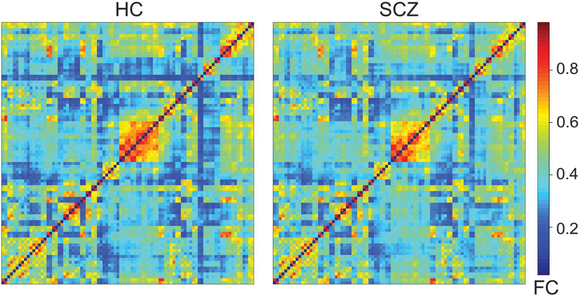
Average connectivity matrices calculated by using pFC. The axis are the labels from the AAL 90 template. HC, healthy control; pFC, pure functional connectivity; SCZ, schizophrenia. Color images are available online.

FD model

A brain network was calculated for each subject [see Equation (1)]. The average whole-brain network per group is depicted in Figure 2-top. Then, pairwise group comparisons were performed in the whole-brain network; the p-values (Fig. 2-bottom) were thresholded at 5% and corrected for multiple comparison (Bonferroni).

FIG. 2.

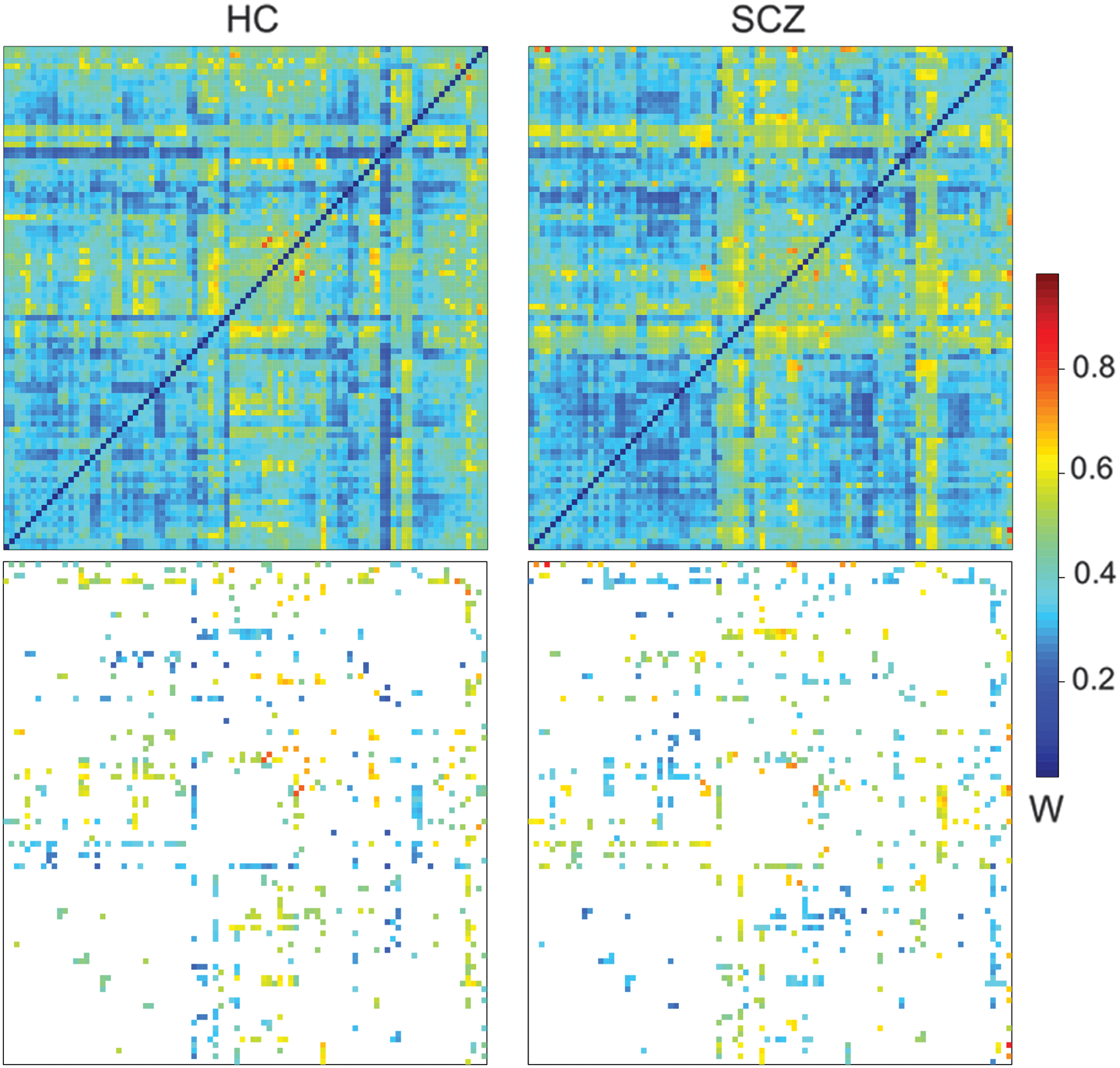
Top—Averaged connectivity matrices calculated by using the FD model. Bottom—Significant links after multiple comparison correction. The axis displays the labels from the AAL 90 template. Connections that were statistically different between healthy control and schizophrenic patients, thresholded by using the Bonferroni-adjusted p-value 0.05. Links are colored according to their average connectivity. FD, F (the functional connectivity matrix) and D (the structural matrix). Color images are available online.

To explore the remaining links after the correction for multiple comparison, we reported the main nodes detected for having a high number of significant links when comparing patient and control groups (Fig. 3 and Table 2). These brain regions were the thalamus, inferior temporal gyrus, middle occipital gyrus, parahippocampus, and superior occipital gyrus. They play a central role in the network given their interconnections and higher differences between schizophrenic and healthy controls. The thalamus was the main hub connecting both cortical (mainly occipital and temporal via superior occipital gyrus) and subcortical areas (parahippocampal gyrus, hippocampus, and precuneus). Impaired connections in frontal areas and sensorimotor cortex were also found. These links were mainly from/to inferior temporal and middle occipital. Interestingly, the hyperconnected subnetwork is part of a large network, known as the thalamo-cortical network (Woodward et al., 2012).

FIG. 3.

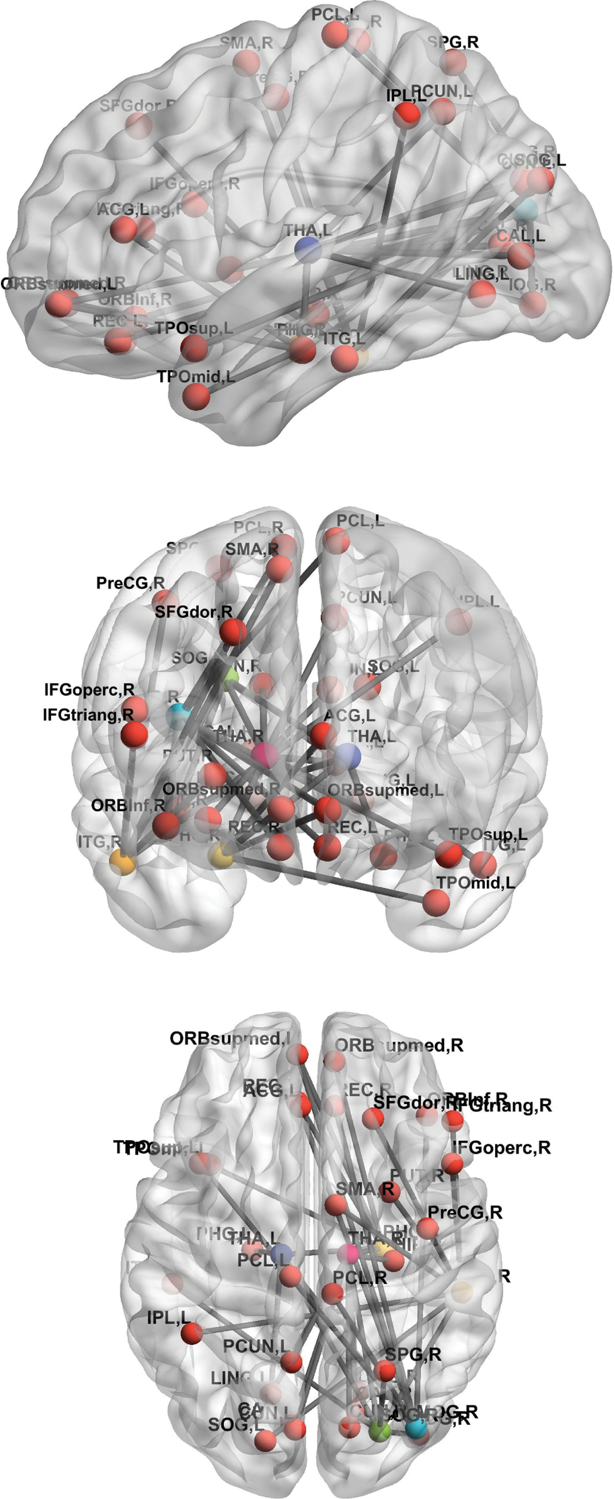
Impaired connections between healthy controls and schizophrenic patients. The central nodes of disrupted subnetworks were THA, ITG, midOG, PHG and SOG. The THA is considered the main hub of these central nodes connecting both cortical (mainly occipital and temporal via SOG) and subcortical areas (PHG, HIP, and PCUN). Impaired connections in frontal areas and sensorimotor cortex were mainly from/to inferior temporal and middle occipital. ACG, anterior cingulum; HIP, hippocampus; ITG, inferior temporal gyrus; L, left; LING, lingual gyrus; midOG, middle occipital gyrus; ORB, orbital; PCL, paracentral lobule; PCUN, precuneus; PHG, parahippocampal gyrus; PreCG, precentral gyrus; R, right; REC, rectus; SFG, superior frontal gyrus; SMA, supplementary motor area; SOG, superior occipital gyrus; SPG, superior parietal gyrus; THA, thalmus; TPO, temporal pole. Color images are available online.

Table 2.

Impaired Links Established by the Central Nodes of the Subnetwork

Central nodes with impaired connectivity	Connected to
Right thalamus	Right hippocampus
	Right parahippocampal gyrus
	Bilateral calcarine
	Bilateral cuneus
	Bilateral lingual gyri
	Right superior occipital gyrus
	Left precuneus
Right inferior temporal gyrus	Right precentral
	Right frontal superior
	Right inferior frontal pars opercularis
	Right frontal inferior pars triangularis
	Right supperior motor areas
	Bilateral superior occipital gyri
	Left inferial parietal gyrus
	Right putamen
Right middle occipital gyrus	Right inferior frontal pars orbitalis
	Left medial frontal pars orbitalis
	Bilateral rectus
	Bilateral paracentral lobuli
	Left superior temporal pole
Right parahippocampus	Bilateral medial frontal pars orbitalis
	Left anterior cingulum
	Bilateral thalamus
	Left middle temporal pole
Right superior occipital gyrus	Right inferior occipital gyrus
	Right superior parietal gyrys
	Bilateral thalamus
	Bilateral inferior temporal gyrus
Left thalamus	Bilateral parahippocampal gyri
	Left lingual gyrus
	Right superior occipital gyrus
	Right inferior occipital gyrus

Model comparison: pFC and FD

As shown in the previous section, differences emerged between schizophrenic patients and healthy controls when applying the FD model, whereas these differences were not detected while employing the pFC model.

In this section, to support the outcomes, we provided a statistical comparison between the two approaches. For that, the following steps were considered.

Test the null hypothesis that the links found by the two models were the same. To this, we considered all the available connections (positive correlations), namely the original adjacency matrices associated to the two models (F for the pFC and W for the FD).

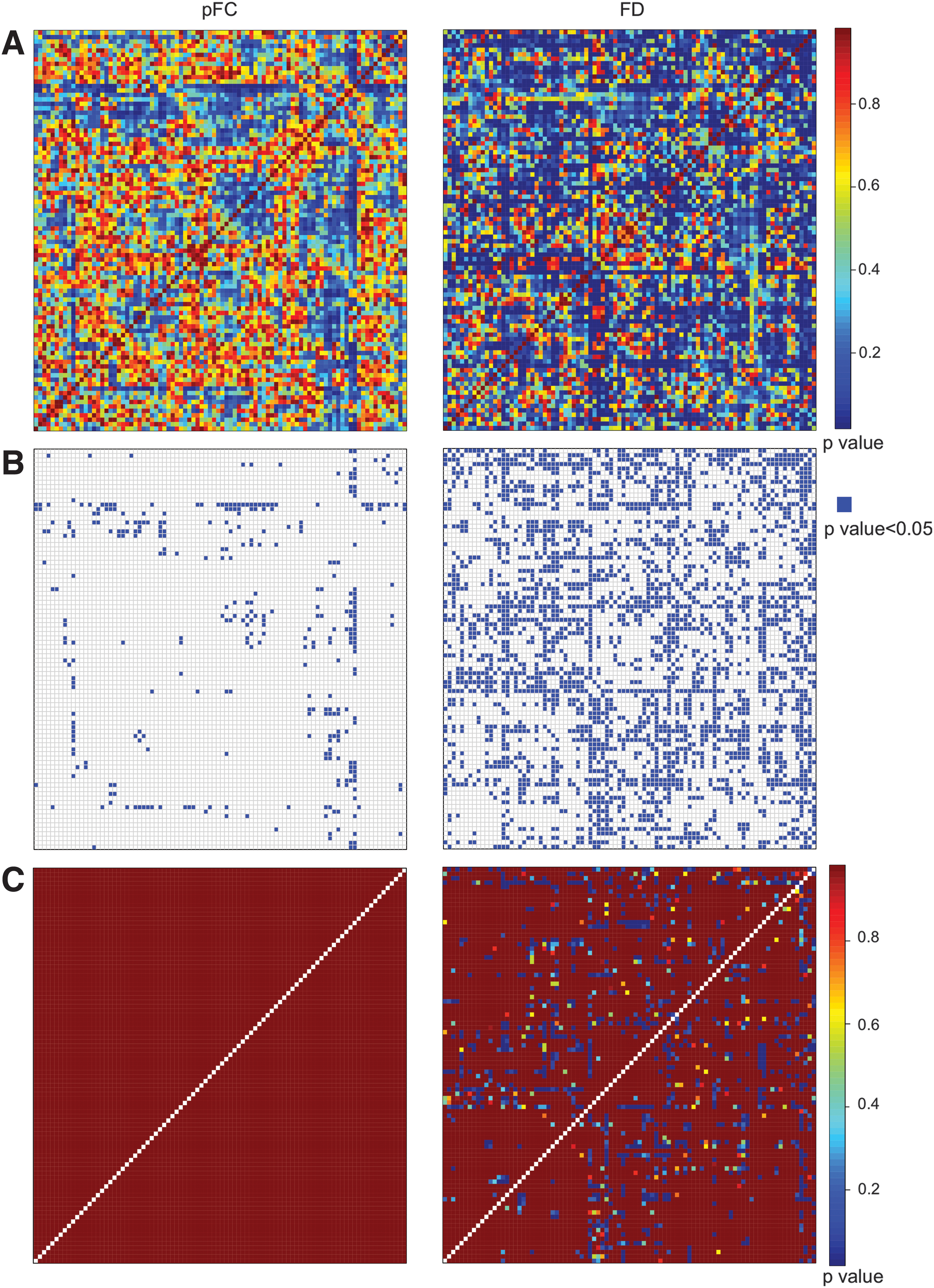
From F and W, we computed the corresponding unadjusted p-values (Fig. 4A-left and right, respectively).

To avoid statistically nonsignificant links, we fixed the threshold α = 0.05 and removed all links having unadjusted p-values greater than α (Fig. 4B-left and right, respectively).

Since multiple tests were required, we then applied a Bonferroni-Holm statistical correction to the unadjusted p-values matrices previously obtained (Fig. 4C-left and right, respectively). Note that, after such an adjustment, all p-values computed for the pFC model are equal to 1, meaning that no statistically significant differences can be outlined by the pFC model between healthy control and schizophrenic patients. Differently, by employing the FD model, a considerable amount of statistically significant differences can be detected between the two groups.

To test whether the links found by applying the FD model were the same as the ones revealed by applying the standard pFC analysis, that is, whether there was a significant overlap between the links found by the two methods, we calculated the confusion matrix (Table 3). On the two rows of the confusion matrix, the nonsignificant and the significant links according to the FD model are reported; on the columns, the nonsignificant and the significant links according to the pFC model are reported. In particular, on the main diagonal of Table 3, the percentages of overlapping links in the two analyses are shown; whereas, on the other diagonal, the percentages of nonoverlapping links are shown.

FIG. 4.

(A) Adjacency matrix with uncorrected p-values for FD model (right column) and pFC model (left column). (B) Adjacency matrix with thresholded uncorrected p-values at 5%. (C) Bonferroni-Holm adjusted p-values for the FD model (right column) and the pFC model (left column). There were no significant differences in connectivity for the pFC model between healthy controls and schizophrenic patients. The axis contains the labels from the AAL 90 template. Color images are available online.

Table 3.

Confusion Matrix: Overlapping Links Between FD Model and Pure Functional Connectivity Model

	Nonsignificant pFC	Significant pFC
Nonsignificant W FD	5099 (63%)	127 (1.6%)
Significant W FD	2651 (33%)	223 (2.8%)

Bold indicates the links that are non-significant (63%) and significant (2.8%) for both FD and pFC models.

FD, F (the functional connectivity matrix) and D (the structural matrix); pFC, pure functional connectivity.

Most of the links were nonsignificant for both models: 5099 (63%). The number of links that were significant for the FD model and for the pFC model was 223 (2.8%; Supplementary Fig. S1). The links that were significant for the FD model but not for the pFC model summed up to 2651 (33%). Significant links for pFC that were not in FD corresponded to 127 (1.6%).

The low percentage of links that were significant in both models can be explained by the low percentage of links that were detected by the pFC model (1.6% +2.8% = 4.4%). This issue might be ascribed to the possibly low statistical power of the tests performed, in relation to the number and heterogeneity of individuals in the sample. Despite statistical power issues, a relevant percentage of significant links (33% +2.8% = 35.8%) could be detected by the FD model. In addition, when considering the total links detected by the pFC model (4.4%), 65% of them are also detected by the FD model.

FD and pFC using Harvard-Oxford atlas

The same procedures described earlier were applied by using the Harvard-Oxford atlas. After correcting for multiple comparisons, there was no remaining links in the pFC model, as also seen in the AAL atlas. Likewise, the thalamo-cortical network was impaired in schizophrenic patients: The thalamus was connected to the superior frontal gyrus, inferior frontal gyrus (pars triagularis), parahipocampal gyrus (posterior division), hippocampus, cuneal cortex, temporal fusiform cortex (posterior division), and occipital pole.

Discussion

We applied a new model, called the FD model, to infer connectivity in the brain and compared it with the classical pFC model. The main advantage of the FD model is that it not only takes into consideration the temporal correlations, as pFC does, but also includes information about inferred structural connectivity and topological information of the network. Combining structural and functional information, two equally important features of the brain, might give rise to more realistic and even reliable models of brain networks (Battiston et al., 2017; Bowman et al., 2012; Calamante et al., 2017; Calhoun and Sui, 2016; Chu et al., 2018; Kang et al., 2017; Xue et al., 2015). In addition, degree is an important topological measure that reflects how well a specific region is connected to the whole network and it is, therefore, related to the notion of a hub. Hubs play a central role in the network, integrating and distributing information in effective ways due to the number and positioning of their connections in a network.

Once the models were applied to each subject in the schizophrenic group and in the healthy controls, individual whole-brain networks were inferred followed by a pairwise comparison of all connections in the network between groups. In the FD model, we found widespread disrupted connectivity in key areas for schizophrenia (Andreasen, 1997; Andreasen et al., 1998; Pergola et al., 2015), namely, hyperconnectivity in the thalamo-cortical network: thalamus, occipital, temporal parahippocampal gyrus, and frontal areas. In this network, there were six main central nodes: bilateral thalamus, right parahippocampal gyrus, right superior and middle occipital, and right inferior temporal gyrus. In addition, frontal and somatosensory areas were also present; in this case, the impaired connections arise mainly from the temporal inferior hub and middle occipital hub.

In line with previous models such as the “cognitive dysmetria” (Andreasen et al., 1998) and “filtering” models (Pergola et al., 2015), we observed that the thalamus was the main hub of the disrupted network. This region is located in a crucial anatomic position of the brain and its main function is the facilitation of connections as it receives input and output from distinct cortical areas. For this reason, it has been considered a key player in filtering and gating of information (Andreasen, 1997; Pergola et al., 2015). Further, it has been suggested that the thalamus might play a crucial role in schizophrenia because any disconnection in such a gate could lead to major changes in information load (Andreasen, 1997), which, in turn, might account for the great variety of cognitive and clinical characteristics of the disease (Andreasen et al., 1998). Motivated by patients' description of “being bombed by stimuli which they have difficulty screening out” (McGhie and Chapman, 1961), Andreasen (Andreasen, 1997) hypothesized a scenario in which information overload due to filtering and gating dysfunction could lead to a misinterpretation of the “self/not self,” auditory hallucinations, persecution, lack of energy, etc., that represent key symptoms of schizophrenia. Although a growing body of evidence points to disruptions in the thalamus in schizophrenic patients (Ferri et al., 2018; Pergola et al., 2015), its role and contribution are still a matter of debate.

In the computational neuroscience literature, the thalamus has been reported as a promising candidate for pattern classification analysis (Pergola et al., 2015). In addition, changes in the network topology of schizophrenic patients makes hubs ideal candidates for machine learning techniques as demonstrated by Cheng and colleagues (2015) with high accuracy when classifying patients and controls.

These are exciting outcomes since the declared goal of computational psychiatry is to provide physicians with tools that enable them to objectively identify patients in whom most approaches had been subjective up until that point. The hope is that the computational approach could be used to predict the likelihood of a previously unseen patient having schizophrenia. Identifying topological markers could lead to tools that enable to quantitatively determine the severity of common symptoms and even identify and measure the progression of the disease, as well as the effectiveness of treatment. Hence, it would be of scientific interest to find prognostic and diagnostic markers, not only based on empirical observations but also based on outcomes obtained by a graph theoretical analysis. Our future research will focus on potential biomarkers and classification in schizophrenia.

Comparing the FD network and pFC network based on pFC, we showed in this study that the FD model is able to select links, of neurobiological meaning for schizophrenia, that otherwise would be neglected by the pFC analysis. Hence, the FD model stresses relevant features of the whole-brain connectivity by adding structural as well as topological information to pFC. Therefore, we suggest that the FD model could be considered as an additional effective model to describe functional neural networks.

We believe that increasing the precision of the anatomical data in the model will reveal even further connectivity differences. In addition, it might contribute to a better understanding about the relationship between structural modularity and functional modularity of the brain, which is an open and challenging problem. Lastly, it is important to stress that the FD model is not only limited to the modality of fMRI. It can be also applied to positron emission tomography, EEG, and magneto-encephalography data.

Footnotes

Acknowledgments

C.G.F. would like to thank Dr. Leonie Ascone Michelis for fruitful discussion about the role of the thalamo-cortical network in schizophrenia.

S.K. was funded by two grants from the German Science Foundation (DFG KU 3322/1-1, SFB 936/C7), the European Union (ERC-2016-StG-Self-Control-677804) and a Fellowship from the Jacobs Foundation (JRF 2016–2018). CGF was funded by the German Science Foundation (SFB 936/C7). L.K. was funded by the Evangelisches Studienwerk Villigst.

Authors' Contribution

Data acquisition: L.K., J.B., L.S., P.G., M.F., N.S., C.M., S.K., J.G. Data analysis: C.G.F., P.F., A.P., S.K., P.D. Article writing: C.G.F., P.F., A.P., J.G., S.K., P.D.

Author Disclosure Statement

No competing financial interests exist.

Supplementary Material

Supplementary Figure S1

References

Abrol

, Rashid

, Rachakonda

, Damaraju

, Calhoun

. 2017. Schizophrenia shows disrupted links between brain volume and dynamic functional connectivity. Front Neurosci, 11:624.

Ackenheil

, Stotz-Ingenlath

, Dietz-Bauer

, Vossen

. 1999. MINI Mini International Neuropsychiatric Interview, German Version 5.0.0, DSM IV. München, Germany: Psychiatrische Universitätsklinik München.

Andreasen

. 1984. The Scale for the Assessment of Positive Symptoms (SAPS). Iowa City, Iowa: University of. Iowa.

Andreasen

. 1989. Scale for the assessment of negative symptoms (SANS). Conceptual and theoretical foundations. Br J Psychiatry, 155:49–52.

Andreasen

. 1997. The role of the thalamus in schizophrenia. Can J Psychiatry, 42:27–33.

Andreasen

, Paradiso

, O'Leary

. 1998. “Cognitive dysmetria”; as an integrative theory of schizophrenia: a dysfunction in cortical-subcortical-cerebellar circuitry?. Schizophr Bull, 24:203–218.

Andreasen

, Pierson

. 2008. The role of the cerebellum in schizophrenia. Biol Psychiatry, 64:81–88.

Barch

. 2014. Cerebellar-thalamic connectivity in schizophrenia. Schizophr Bull, 40:1200–1203.

Bassett

, Bullmore

, Verchinski

, Mattay

, Weinberger

, Meyer-Lindenberg

. 2008. Hierarchical organization of human cortical networks in health and schizophrenia. J Neurosci, 28:9239–9248.

10.

Battiston

, Nicosia

, Chavez

, Latora

. 2017. Multilayer motif analysis of brain networks. Chaos, 27:047404.

11.

Bowman

, Zhang

, Derado

, Chen

. 2012. Determining functional connectivity using fMRI data with diffusion-based anatomical weighting. Neuroimage, 62:1769–1779.

12.

Calamante

, Smith

, Liang

, Zalesky

, Connelly

. 2017. Track-weighted dynamic functional connectivity (TW-dFC): a new method to study time-resolved functional connectivity. Brain Struct Funct, 222:3761–3774.

13.

Calhoun

, Adali

, Giuliani

, Pekar

, Kiehl

, Pearlson

. 2006. Method for multimodal analysis of independent source differences in schizophrenia: combining gray matter structural and auditory oddball functional data. Hum. Brain Mapp, 27:47–62.

14.

Calhoun

, Sui

. 2016. Multimodal fusion of brain imaging data: a key to finding the missing link(s) in complex mental illness. Biol Psychiatry Cogn Neurosci Neuroimaging, 1:230–244.

15.

Cheng

, Newman

, Goñi

, Kent

, Howell

, Bolbecker

, et al. 2015. Nodal centrality of functional network in the differentiation of schizophrenia. Schizophr Res, 168:345–352.

16.

Chu

S-H

, Parhi

, Lenglet

. 2018. Function-specific and enhanced brain structural connectivity mapping via joint modeling of diffusion and functional MRI. Sci Rep, 8:4741.

17.

Cocchi

, Harding

, Lord

, Pantelis

, Yucel

, Zalesky

. 2014. Disruption of structure-function coupling in the schizophrenia connectome. Neuroimage Clin, 4:779–787.

18.

Dulio

, Finotelli

, Frosini

, Pergola

, Presenti

. 2018. Graph model simulation of human brain's functional activity at resting state by means of the FD model. Fundam Inform, 163:93–109.

19.

Ferri

, Ford

, Roach

, Turner

, van Erp

, Voyvodic

, et al. 2018. Resting-state thalamic dysconnectivity in schizophrenia and relationships with symptoms. Psychol Med, 48:2492–2499.

20.

Finotelli

, Dipasquale

, Costantini

, Pini

, Baglio

, Baselli

, et al. 2018. Exploring resting-state functional connectivity invariants across the lifespan in healthy people by means of a recently proposed graph theoretical model. PLoS One, 13:e0206567.

21.

Finotelli

, Dulio

. 2015. A Mathematical model for evaluating the functional connectivity strongness in healthy people. Arch Ital Biol, 153:279–300.

22.

Finotelli

, Panzica

, Dulio

, Rotondi

, Varotto

. 2016. A statistical proposal for selecting a data-depending threshold in neurobiology. Arch Ital Biol, 154:78–101.

23.

Friston

. 1999. Schizophrenia and the disconnection hypothesis. Acta Psychiatr Scand, 99:68–79.

24.

Friston

, Frith

. 1995. Schizophrenia: a disconnection syndrome?. Clin Neurosci, 3:89–97.

25.

García-Martí

, Aguilar

, Martí-Bonmatí

, Escartí

, Sanjuán

. 2012. Multimodal morphometry and functional magnetic resonance imaging in schizophrenia and auditory hallucinations. World J Radiol, 4:159–166.

26.

Garrity

, Pearlson

, McKiernan

, Lloyd

, Kiehl

, Calhoun

. 2007. Aberrant “default mode” functional connectivity in schizophrenia. Am J Psychiatry, 164:450–457.

27.

Guo

, Huang

C-C

, Zhao

, Yang

, Lin

C-P

, Nichols

, Tsai

S-J

. 2018. Combining multi-modality data for searching biomarkers in schizophrenia. PLoS One, 13:e0191202.

28.

Hadley

, Kraguljac

, White

, Ver Hoef

, Tabora

, Lahti

. 2016. Change in brain network topology as a function of treatment response in schizophrenia: a longitudinal resting-state fMRI study using graph theory. NPJ Schizophr, 2:16014.

29.

, Chen

, Evans

. 2007. Small-world anatomical networks in the human brain revealed by cortical thickness from MRI. Cereb Cortex, 17:2407–2419.

30.

Kang

, Ombao

, Fonnesbeck

, Ding

, Morgan

. 2017. A Bayesian double fusion model for resting-state brain connectivity using joint functional and structural data. Brain Connect, 7:219–227.

31.

Keefe

RSE

, Harvey

, Goldberg

, Gold

, Walker

, Kennel

, Hawkins

. 2008. Norms and standardization of the Brief Assessment of Cognition in Schizophrenia (BACS). Schizophr Res, 102:108–115.

32.

Kühn

, Romanowski

, Schubert

, Gallinat

. 2012. Reduction of cerebellar grey matter in Crus I and II in schizophrenia. Brain Struct Funct, 217:523–529.

33.

Lerch

, Worsley

, Shaw

, Greenstein

, Lenroot

, Giedd

, Evans

. 2006. Mapping anatomical correlations across cerebral cortex (MACACC) using cortical thickness from MRI. Neuroimage, 31:993–1003.

34.

Liu

, Wang

, Song

, Lv

, Cui

, Liu

, et al. 2019. Linked 4-Way multimodal brain differences in schizophrenia in a large Chinese Han population. Schizophr Bull, 45:436–449.

35.

McGhie

, Chapman

. 1961. Disorders of attention and perception in early schizophrenia. Br J Med Psychol, 34:103–116.

36.

Mechelli

, Price

, Friston

, Ashburner

. 2005. Voxel-based morphometry of the human brain: methods and applications. Curr Med Imaging Rev, 1:105–113.

37.

Nelson

, Bassett

, Camchong

, Bullmore

, Lim

. 2017. Comparison of large-scale human brain functional and anatomical networks in schizophrenia. Neuroimage Clin, 15:439–448.

38.

Nelson

, Saykin

, Flashman

, Riordan

. 1998. Hippocampal volume reduction in schizophrenia as assessed by magnetic resonance imaging. Arch Gen Psychiatry, 55:433.

39.

Pergola

, Selvaggi

, Trizio

, Bertolino

, Blasi

. 2015. The role of the thalamus in schizophrenia from a neuroimaging perspective. Neurosci Biobehav Rev, 54:57–75.

40.

Power

, Barnes

, Snyder

, Schlaggar

, Petersen

. 2012. Spurious but systematic correlations in functional connectivity MRI networks arise from subject motion. Neuroimage, 59:2142–2154.

41.

, Sui

, Chen

, Liu

, Jiang

, Silva

, et al. 2019. Parallel group ICA+ICA: joint estimation of linked functional network variability and structural covariation with application to schizophrenia. Hum Brain Mapp [Epub ahead of print]; DOI: 10.1002/hbm.24632.

42.

Qureshi

MNI

, Oh

, Cho

, Jo

, Lee

. 2017. Multimodal discrimination of schizophrenia using hybrid weighted feature concatenation of brain functional connectivity and anatomical features with an extreme learning machine. Front Neuroinform, 11:59.

43.

Schmidt

, Metzler

. 1992. Wortschatztest (WST). Weinheim, Germany:. Beltz.

44.

Singh

, Modi

, Goyal

, Kaur

, Singh

, Bhatia

,. 2015. Functional and structural abnormalities associated with empathy in patients with schizophrenia: an fMRI and VBM study. J Biosci, 40:355–364.

45.

Song

X-W

, Dong

Z-Y

, Long

X-Y

, Li

S-F

, Zuo

X-N

, Zhu

C-Z

, et al. 2011. REST: a toolkit for resting-state functional magnetic resonance imaging data processing. PLoS One, 6:e25031.

46.

Sui

, Pearlson

, Du

, Yu

, Jones

, Chen

, et al. 2015. In search of multimodal neuroimaging biomarkers of cognitive deficits in schizophrenia. Biol Psychiatry, 78:794–804.

47.

Tzourio-Mazoyer

, Landeau

, Papathanassiou

, Crivello

, Etard

, Delcroix

, et al. 2002. Automated anatomical labeling of activations in SPM using a macroscopic anatomical parcellation of the MNI MRI single-subject brain. Neuroimage, 15:273–289.

48.

van den Heuvel

, Fornito

. 2014. Brain networks in schizophrenia. Neuropsychol Rev, 24:32–48.

49.

van den Heuvel

, Hulshoff Pol

. 2010. Exploring the brain network: a review on resting-state fMRI functional connectivity. Eur Neuropsychopharmacol, 20:519–534.

50.

Wang

, Meda

, Keshavan

, Tamminga

, Sweeney

, Clementz

, et al. 2015. Large-scale fusion of gray matter and resting-state functional MRI reveals common and distinct biological markers across the psychosis spectrum in the B-SNIP cohort. Front Psychiatry, 6:174.

51.

Woodward

, Karbasforoushan

, Heckers

. 2012. Thalamocortical dysconnectivity in schizophrenia. Am J Psychiatry, 169:1092–1099.

52.

Xue

, Bowman

, Pileggi

, Mayer

. 2015. A multimodal approach for determining brain networks by jointly modeling functional and structural connectivity. Front Comput Neurosci, 9:22.

53.

Zalesky

, Fornito

, Egan

, Pantelis

, Bullmore

. 2012. The relationship between regional and inter-regional functional connectivity deficits in schizophrenia. Hum Brain Mapp, 33:2535–2549.

Supplementary Material

Please find the following supplemental material available below.

For Open Access articles published under a Creative Commons License, all supplemental material carries the same license as the article it is associated with.

For non-Open Access articles published, all supplemental material carries a non-exclusive license, and permission requests for re-use of supplemental material or any part of supplemental material shall be sent directly to the copyright owner as specified in the copyright notice associated with the article.

0.00 MB

0.06 MB