Effect of Fixed-Density Thresholding on Structural Brain Networks: A Demonstration in Cerebral Small Vessel Disease

Abstract

A popular solution to control for edge density variability in structural brain network analysis is to threshold the networks to a fixed density across all subjects. However, it remains unclear how this type of thresholding affects the basic network architecture in terms of edge weights, hub location, and hub connectivity and, especially, how it affects the sensitivity to detect disease-related abnormalities. We investigated these two questions in a cohort of patients with cerebral small vessel disease and age-matched controls. Brain networks were reconstructed from diffusion magnetic resonance imaging data using deterministic fiber tractography. Networks were thresholded to a fixed density by removing edges with the lowest number of streamlines. We compared edge length (mm), fractional anisotropy (FA), proportion of hub connections, and hub location between the unthresholded and the thresholded networks of each subject. Moreover, we compared weighted graph measures of global and local connectivity obtained from the (un)thresholded networks between patients and controls. We performed these analyses over a range of densities (2–20%). Results indicate that fixed-density thresholding disproportionally removes edges composed of long streamlines, but is independent of FA. The edges removed were not preferentially connected to hub or nonhub nodes. Over half of the original hubs were reproducible when networks were thresholded to a density ≥10%. Furthermore, the between-group differences in graph measures observed in the unthresholded network remained present after thresholding, irrespective of the chosen density. We therefore conclude that moderate fixed-density thresholds can successfully be applied to control for the effects of density in structural brain network analysis.

Introduction

Studies of brain network changes in disease have improved our understanding of a wide range of cognitive and neurological disorders (Bassett and Bullmore, 2009; Stam, 2014). In network neuroscience, the structural brain network is often described as a set of nodes (gray matter regions) connected by edges (white matter tracts). Then, graph theoretical analysis is applied to characterize this network, allowing us to examine topological differences between patients and controls (Liu et al., 2017; Rubinov and Sporns, 2010; Sporns et al., 2005).

Although methods to reconstruct brain networks are improving, several methodological issues remain (Qi et al., 2015; Stam, 2014). A well-known issue is the confounding effect of network density (i.e., the number of detected edges divided by the number of all possible edges) on graph metrics (Stam, 2014; van Wijk et al., 2010). Since graph metrics are mathematically dependent on network density, variation in density caused by factors unrelated to disease of interest can mask real group differences or introduce false group differences (van Wijk et al., 2010). Such unwanted variation can be caused by factors related to network reconstruction. For example, brain networks reconstructed from diffusion magnetic resonance imaging (MRI) data contain false-positive and false-negative connections due to errors in fiber tractography, which occur especially in white matter regions with complex fiber orientations (Hein et al., 2016; Jeurissen et al., 2017). These complex fiber orientations cannot be fully resolved by using the diffusion tensor model, resulting in early termination of fiber tracts (i.e., false negatives) (Jones, 2008). On the contrary, advanced diffusion models such as constrained spherical deconvolution (CSD) are more effective in resolving complex fiber orientations but are prone to detect many false positives (Zalesky et al., 2016). Altogether, these reconstruction errors contribute to the variation in network density across subjects, affecting the computation and comparison of graph metrics.

One of the most straightforward methods to control for the variability in network density is to threshold the connectivity matrix by removing edges with the lowest weight until a common fixed density is achieved across all individuals (Achard and Bullmore, 2007; Bassett et al., 2009; van den Heuvel et al., 2008). Fixed-density thresholding is widely used in functional connectivity studies and has been suggested to be more reliable than other thresholding approaches such as absolute thresholding (Mårtensson et al., 2018; Telesford et al., 2011). However, the advantages and shortcomings of fixed-density thresholding are still under discussion (Garrison et al., 2015; van den Heuvel et al., 2017; Váša et al., 2018).

Much less is known about the consequences of fixed-density thresholding on diffusion-based brain networks (Andreotti et al., 2014b; Drakesmith et al., 2015). In particular, the effect of thresholding on the basic architecture of diffusion-based networks (e.g., edge composition, location of hub nodes and hub connections) is still unclear. The influence of thresholding on these network properties is relevant since these characteristics are the building blocks of structural networks and are often the focus of clinical studies (Achard et al., 2012; Daianu et al., 2016; Pandit et al., 2013). For example, long-range fiber connections are suggested to be more affected in certain neurological disorders (Daianu et al., 2015). Moreover, network hubs and hub connections are preferentially disrupted in many pathologies, and are frequently the most discriminatory features between patients and controls (Fagerholm et al., 2015; Tuladhar et al., 2017). Thus, before applying fixed-density thresholding in clinical studies, it is essential to understand if and how it affects the edge composition, the organization of hubs and hub connections in the network as well as the subsequent between-group comparisons of graph metrics.

In this study, we assessed the effects of thresholding on (1) edge composition, location of hub nodes and hub connectivity and (2) the ability to detect between-group differences in a cohort of patients with cerebral small vessel disease (SVD). SVD is a common cause of white matter injury in the elderly, and previous studies have characterized network abnormalities in patients with SVD based on unthresholded networks (Heinen et al., 2018; Reijmer et al., 2015). We evaluated our research objectives over a range of network densities while maintaining a fully connected network (van Dellen et al., 2018).

Materials and Methods

Participants

Patients included in this study were part of the TRACE-VCI cohort recruited through the memory clinic at the University Medical Center Utrecht (Boomsma et al., 2017). Inclusion and exclusion criteria of the original cohort are described elsewhere (Boomsma et al., 2017; Heinen et al., 2018). Patients were eligible for this study if they had (1) a structural brain MRI scan, including a diffusion-weighted sequence; (2) evidence of SVD on MRI, such as white matter hyperintensities (WMH) and lacunes; and (3) if they presented with cognitive complaints, resulting in 162 patients.

In addition, 53 age-, sex-, and education-matched elderly without any history of dementia or other known neurological disorder that could affect cognition, and a minimental state examination (MMSE) score between 28 and 30, were included as a control group (Table 1). Control participants were recruited from the population as part of the Utrecht Diabetic Encephalopathy Study (van Den Berg et al., 2010).

Table 1.

Characteristics of the Study Population

	SVD patients, N = 137	Controls, N = 44
Demographic characteristics
Female sex	65 (47.4)	21 (47.7)
Age, in years	74.01 ± 7.88	72.0 ± 4.6
MMSE	26 [23–28]	29 [28–30]^*
Imaging markers
Brain volume in % of ICV	67.5 [64.9–69.3]	70.9 [69.9–73.0]^*
GM volume in % of ICV	35.4 [34.1–36.7]	38.4 [36.5–39.7]^*
WMH volume in % of ICV	1.1 [0.4–2.2]	0.4 [0.2–0.8]^*
Lacunes	46 (34)	13 (30)

Data presented as mean ± standard deviation, absolute number (%), or median [interquartile range].

Demographic variables and MRI markers of SVD were compared between patients and controls using independent-samples t-test for continuous variables and χ² test for proportions. For the MMSE, brain volume, GM volume, and WMH volume, we used the nonparametric equivalent of the independent-samples t-test, Mann–Whitney U test, since these variables were not normally distributed.

p < 0.02.

GM, gray matter; ICV, intracranial volume; MMSE, minimental state examination; MRI, magnetic resonance imaging; SVD, small vessel disease; WMH, white matter hyperintensities.

All participants underwent 1-day clinical examination, neuropsychological assessment, and a 3-T brain MRI. Since the focus of this study was the reconstruction of structural brain networks, we excluded participants with a low-quality diffusion and/or T1 scans (n = 25 patients, n = 9 controls), yielding 137 patients and 44 controls for the current analyses. Low-quality scans were defined by the presence of major signal dropouts, large subject motion, and/or susceptibility distortions. These scans were excluded in hindsight, after we verified that these artifacts could not fully be corrected during the processing pipeline described below. Characteristics of the study population, including the degree of vascular brain injury, are given in Table 1.

The study was approved by the institutional review board of the UMC Utrecht, and all participants provided written informed consent before any research procedure.

Magnetic resonance imaging data acquisition

MRI data of patients and controls were acquired on a 3-T Philips scanner (Achieva, Philips, Best, the Netherlands) using a standardized protocol that included a 3D T1-weighted image and a diffusion-weighted sequence. The T1 scans were acquired with the following parameters: 192 continuous slices, isotropic acquisition voxel size: 1 × 1 × 1 mm³, a flip angle of 8°, echo time (TE): 4.5 ms and repetition time (TR): 7.9 ms.

The diffusion-weighted scans were obtained using a single-shot spin echo EPI sequence with 48 contiguous slices, field of view of 220 × 220 × 120 mm³, isotropic acquisition voxel size: 2.5 × 2.5 × 2.5 mm³, TR/TE 6638/73 ms, 45 isotropically distributed diffusion-sensitizing gradients with a b-value of 1200 s/mm², and 1 b = 0 s/mm² (3 signal averages).

Furthermore, a fluid-attenuated inversion recovery sequence (FLAIR; TR/TE/Inversion time = 11,000/125/2800 ms) was acquired to rate neuroimaging markers of SVD (i.e., brain volumes, WMH volume, and lacunes).

Diffusion MRI processing and fiber tractography

The diffusion-weighted data were processed using ExploreDTI version 4.8.6 (Leemans et al., 2009) running on MATLAB R2014b (MATLAB and Statistics Toolbox Release 2014b; The MathWorks, Inc., Natick, MA). Data were corrected for signal drift (Vos et al., 2017), subject motion, eddy current, and susceptibility artifacts, including rotation of the B-matrix before the estimation of the diffusion tensors (Leemans and Jones, 2009; Tax et al., 2015; Veraart et al., 2013).

The diffusion tensors were computed using robust estimators (Tax et al., 2015) followed by whole-brain tractography. Fiber tracts were reconstructed by starting seed points uniformly throughout the data at 2 mm isotropic resolution with a step size of 1 mm. Each streamline was propagated using integration over fiber orientation distributions (FODs). Streamlines were guided by fiber orientations inferred using CSD with a maximum harmonic order (l-max) of 6. This method allows for the reconstruction of more complex pathways, such as those found in regions of crossing fibers (Jeurissen et al., 2011). Streamlines were terminated when they entered a voxel with FOD <0.1, or when the deflection angle between two successive steps was >45°. These tractography parameters were chosen according to recommendations from the previous literature (Jeurissen et al., 2017).

Network reconstruction

The T1-weighted images were preprocessed using the Computational Anatomy Toolbox (CAT12) from SPM. The pipeline, as illustrated in Figure 1, included brain extraction and parcellation of the brain volume into 90 cortical and subcortical regions of interest (ROIs), using the automated anatomical labeling (AAL) template (Tzourio-Mazoyer et al., 2002). The parcellation was performed in the native space, with the AAL template being warped to each subject's T1 image (Odish et al., 2015). After parcellation, we visually checked the quality of each image, and overlaid the segmented AAL labels with the original T1 image to ensure that the registration and parcellation were successful. The cerebellum was excluded from the analysis since most subjects had insufficient scan coverage of this structure.

FIG. 1.

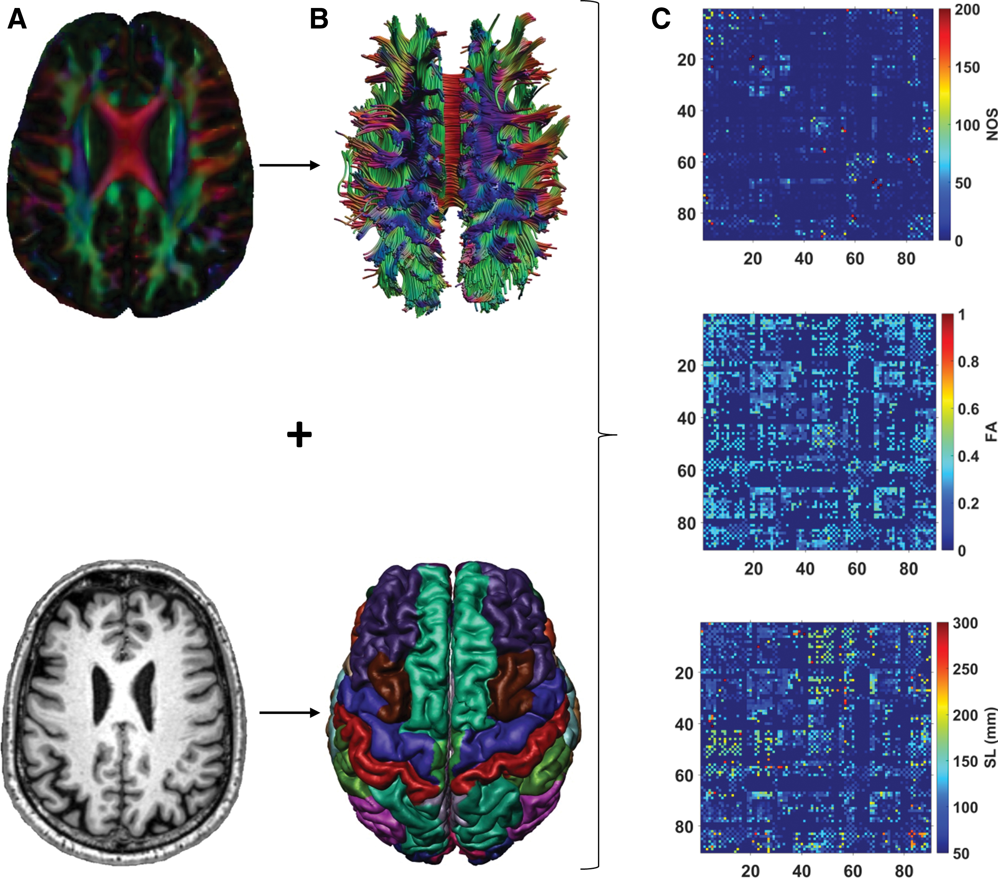
Flowchart of the structural network reconstruction. (A) Coregistration of the diffusion-weighted image (top) with the T1-weighted image (bottom). (B) Reconstruction of fiber tracts from the diffusion-weighted data (top) and the parcellation of the T1 image into 90 cortical and subcortical regions using AAL template (bottom). (C) Network definition: for any pair of ROIs of the AAL template, we established that a connection was present when at least one streamline existed with end-points in these two regions, resulting in a 90 × 90 connectivity matrix; NOS-weighted matrix (top), FA-weighted matrix (middle), SL-weighted matrix (bottom). AAL, automated anatomical labeling; FA, fractional anisotropy; NOS, number of streamlines; ROIs, regions of interest; SL, streamline length. Color images are available online.

For network definition, each ROI represented a node in the network. Two nodes were considered to be connected if they contained the end-points of at least one streamline, resulting in a 90 × 90 binary connectivity matrix. We also obtained three weighted connectivity matrices for each subject, in which the previously defined edges were weighted by the number of streamlines (NOS), average streamline length (SL), and fractional anisotropy (FA) (Fig. 1).

Network thresholding

The NOS-weighted matrix is typically used for thresholding (Sarwar et al., 2019; van Dellen et al., 2018). To obtain thresholded networks, edges with the lowest NOS are removed, which can result in disconnected networks. To ensure that the network did not become disconnected, we first calculated the minimum spanning tree (MST) using the Kruskal algorithm (Kruskal, 1956). The MST is an acyclic subgraph that connects all N nodes in the network such that the weight is minimal. We computed the MST by selecting the edges with the largest NOS first. This method of constructing the MST has previously been described as a good representation of the network backbone (Tewarie et al., 2015; van Dellen et al., 2018). The MST has per definition N − 1 edges and a density of 2/N. Since our network definition includes N = 90 nodes, the density of the MST was ≈2.2%.

To obtain networks with larger densities, we added edges from the original unthresholded network to the MST, until a fixed density was reached, again by selecting edges with the largest NOS first. After each thresholding step, the NOS weights were disregarded to obtain binary matrices with densities of 2.2% (MST), 5%, 10%, 15%, and 20% (Fig. 2). In this manner, the NOS weight determined which edges were retained after thresholding. The binary matrices were then multiplied with the FA-weighted and SL-weighted matrices for further analyses.

FIG. 2.

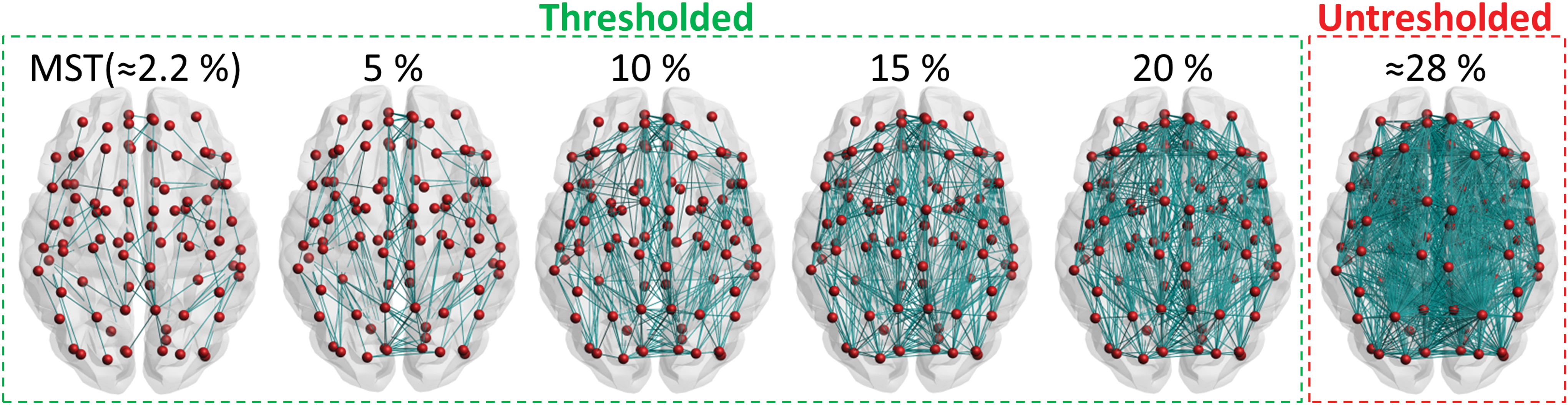
Network thresholding. The first step was the calculation of the MST (density ≈2.2%), by prioritizing the edges with the largest NOS. Next, edges were added until fixed densities of 5%, 10%, 15%, and 20% were reached. The average density of all the unthresholded networks of patients and controls was 28% ± 3% (mean ± SD). MST, minimum spanning tree; SD, standard deviation. Color images are available online.

Edge composition and hubs

The first question we addressed was whether and how thresholding affects the characteristics of edges and nodes in the network. To examine the edge composition, we computed NOS, SL (mm), and FA of the edges removed versus the edges retained in the network.

We also explored whether the edges removed and retained during thresholding were preferentially connected to hub nodes. For this purpose, we first defined hub nodes as the nine nodes with the highest betweenness centrality (i.e., top 10th percentile) (Reijmer et al., 2015). Nodes with high betweenness centrality are often considered “hubs” because they participate in many shortest paths and largely contribute to the global efficiency of the network (Hagmann et al., 2008; van den Heuvel and Sporns, 2011). After defining the hub nodes, we computed the percentage of hub connections relative to all edges retained in the network. Here, hub connections represent edges that connect hub nodes to other hub nodes and edges that connect hub nodes to nonhub nodes. We repeated the calculation of hub connections for each density level.

We also examined whether the hub nodes defined in the unthresholded network corresponded to the hub nodes defined in the thresholded networks. We computed nine hubs (according to the definition above) for each density level and compared their location with the location of the hubs in the unthresholded network. Finally, we investigated whether the overall nodal ranking (here defined as the ranked betweenness centrality of all nodes) was affected by thresholding. We calculated the nodal ranking for each density and compared it with the nodal ranking of the unthresholded network.

Detection of small vessel disease-related network impairments

The second question we addressed was whether thresholding influences comparisons of graph metrics between patients and controls. Ideally, the edge weight applied for thresholding the networks is not the same as applied for the between-group comparisons. In this study, we therefore obtained measures of global connectivity (e.g., global efficiency) and local connectivity (e.g., connectivity strengths of hub and nonhub nodes) from the FA-weighted networks. FA-weighted networks are frequently used to examine structural aspects of brain connectivity in patients and have been shown to be sensitive to the effects of SVD (Heinen et al., 2018; Lawrence et al., 2014; Reijmer et al., 2015; Tuladhar et al., 2016).

Global efficiency was defined as the inverse of the shortest path lengths (i.e., the minimum number of connections between each pair of brain regions). This network measure expresses the extent to which information is exchanged over the network (Rubinov and Sporns, 2010). Connectivity strength of hubs and nonhubs was defined as the mean FA over all the edges connected to hub nodes or nonhub nodes, respectively.

All graph measures mentioned in this article were calculated using the brain connectivity toolbox (https://sites.google.com/site/bctnet) (Rubinov and Sporns, 2010).

SVD imaging markers

SVD markers were computed as described previously (Ferro et al., 2019). Shortly, brain volumes were obtained using an in-house semiautomated pipeline as follows: (1) automated WMH segmentation using the FLAIR images; (2) lesion filling of 3D T1 images; and (3) probabilistic segmentations for gray matter, WM, and CSF. We visually checked the tissue classifications to ensure that the segmentations were correct and not affected by partial volume effects. Total brain volume was defined as the sum of the gray and WM volume. Brain volume was expressed as a percentage of the total intracranial volume. Lacunes were defined as hypointense areas between 2 and 15 mm on both FLAIR and T1-weighted images with a hyperintense rim on FLAIR images. Ratings were performed in line with the STRIVE (Standards for Reporting Vascular Changes on Neuroimaging) criteria (Wardlaw et al., 2013) under supervision of a neuroradiologist (in training).

Statistical analysis

Statistical analysis was performed using IBM SPSS statistics (IBM Corp. Released 2017, IBM SPSS Statistics for Windows, Version 25.0.; IBM Corp., Armonk, NY). A p-value <0.05 was considered significant. Demographic variables and MRI markers of SVD were compared between patients and controls using independent-samples t-test for continuous variables and χ²-test for proportions. For the MMSE, brain volume, gray matter volume, and WMH volume, we used the nonparametric equivalent of the independent-samples t-test, Mann–Whitney U test, since these variables were not normally distributed. Characteristics of the unthresholded network (i.e., edge weights and network density) were compared between patients and controls using independent-samples t-test.

FA and SL were compared between the edges retained and the edges removed from the network using independent-samples t-test. Changes in the organization of nodes were analyzed in two different ways: first, we computed the one-to-one overlap of hub nodes between the unthresholded network and the thresholded networks; second, we correlated the ranked betweenness centrality of the unthresholded network with the ranked betweenness centrality of the thresholded network using Pearson's correlation coefficient (r). Hence, the hub overlap reflects changes in the location of the nine hubs, while the correlation coefficient reflects changes in nodal ranking of all the nodes.

We analyzed between-group differences (SVD vs. controls) in weighted graph metrics (global efficiency, strength of hub- and nonhub nodes) for each density level using a univariate ANOVA with age and sex as covariates. Effect sizes were defined as Cohen's d, and p-values were adjusted for multiple testing using Bonferroni correction. To examine whether the between-group differences change across density levels, we tested interactions between density × group using a repeated-measures ANOVA with group as between-subject factor and density as within-subject factor. Again, age and sex were used as covariates.

Results

Characteristics of the unthresholded network

Characteristics of the unthresholded networks of patients and controls are shown in Figure 3. The NOS of all edges in the unthresholded network was similar for patients and controls (p > 0.14; Fig. 3A). However, the unthresholded networks of patients were composed of edges with relatively long streamlines (p < 0.001; Fig. 3B) and lower FA (p < 0.001; Fig. 3C). Of note, the edge FA and edge length seemed independent of the NOS (Supplementary Fig. S1). The network density of the unthresholded networks of patients (mean ± SD = 26.98% ± 3.12%) was lower when compared with the unthresholded networks of controls (mean ± SD = 28.78% ± 3.17%) (p = 0.002, Fig. 3D).

FIG. 3.

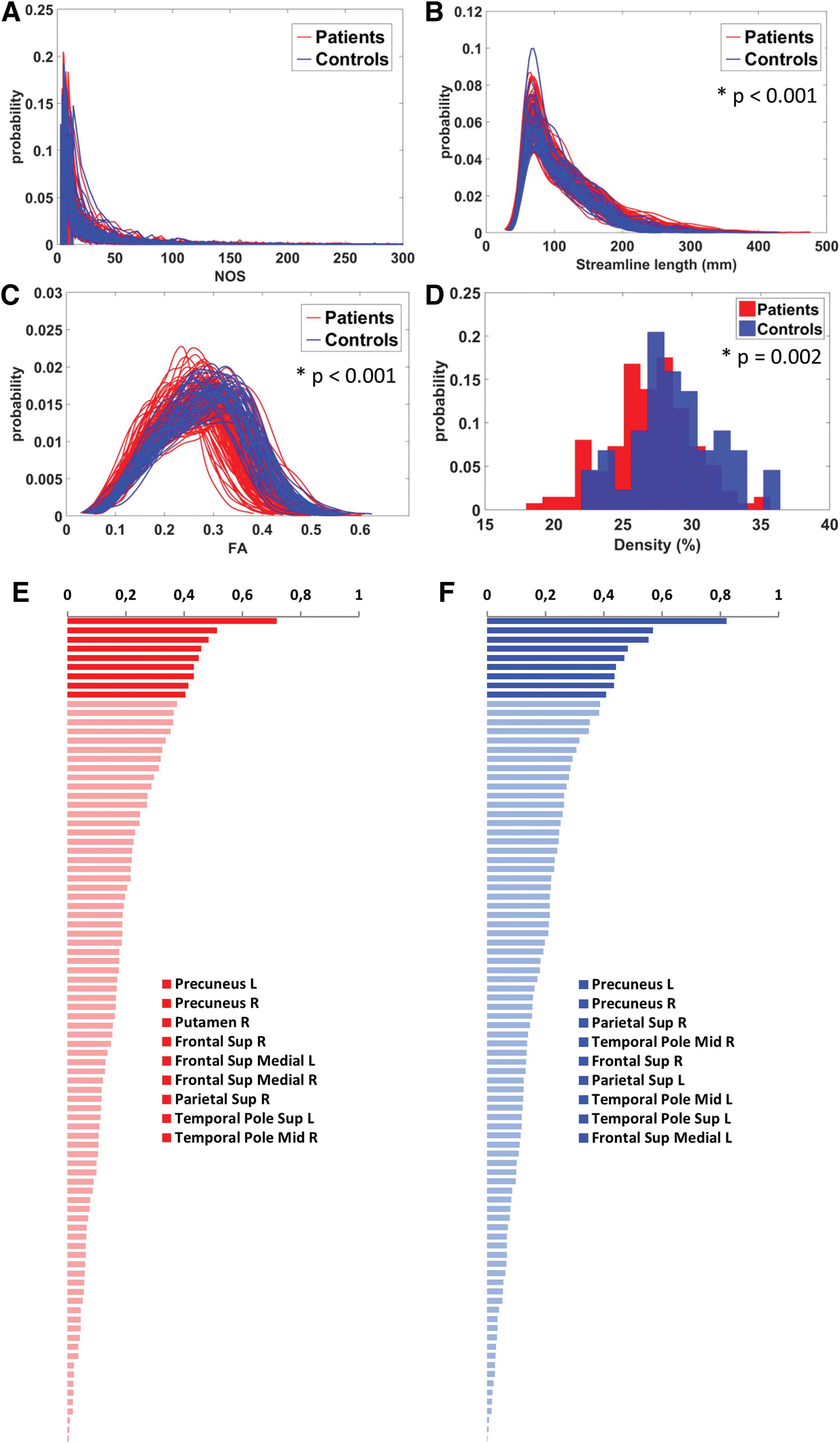
Characteristics of the unthresholded networks. (A) NOS weight of all edges in the unthresholded networks of patients (red) and controls (blue). (B) SL of all edges in the unthresholded networks (patients vs. controls p < 0.001). (C) FA weight of all edges in the unthresholded networks (patients vs. controls p < 0.001). (D) Histogram of network density of the unthresholded networks of patients (mean ± SD = 26.98% ± 3.12%) and controls (mean ± SD = 28.78% ± 3.17%), p = 0.002. (E) Average node betweenness centrality of the unthresholded networks of patients. (F) Average node betweenness of the unthresholded networks of controls. Hubs were defined as the nine nodes with the highest betweenness. Color images are available online.

Nodes that were identified as hubs in the unthresholded networks of patients and controls are shown in Figure 3E and F. Hub nodes were largely consistent across groups and with those commonly reported in the literature (Hagmann et al., 2008; van den Heuvel and Sporns, 2011, 2013).

Effect of thresholding on edge composition and hubs

The effect of thresholding on the edge composition of all subjects is shown in Figure 4. The edges removed from the network during thresholding had, by definition, a lower NOS, but they were also on average longer than the edges retained (p < 0.001; Fig. 4A, B). However, the mean FA was similar for both sets of removed edges (p > 0.10; Fig. 4C).

FIG. 4.

Effect of thresholding on the edge composition. (A) Average NOS of edges retained (black) and edges removed (red) at each density level (all p < 0.001). Error bars represent the SD. “unthr” (unthresholded network). (B) Average SL of the edges retained and edges removed at each density level (all p < 0.001); (C) average FA of the edges retained and the edges removed at each density level (all p > 0.1). p-Values were derived from independent-samples t-tests. Color images are available online.

The effect of thresholding on hub connections and hub nodes of all subjects is shown in Figure 5. In the unthresholded network, 33% of all edges were hub connections (Fig. 5A). This proportion did not change after thresholding, indicating that thresholding did not preferentially target edges connected to hub or nonhub nodes. These results indicate that fixed-density thresholding (based on NOS weights) removes edges composed of relatively long streamlines, but is independent of FA and does not disproportionally affect hub connections. When a small proportion of edges was removed, more than half of the hubs found in the thresholded network corresponded with the original hubs found in the unthresholded network (hub overlap ≥5/9 for densities ≥10%; Fig. 5B). When a greater proportion of edges was removed, the majority of hubs defined in the unthresholded network no longer corresponded with the hubs defined in the thresholded network (hub overlap ≤4/9 for densities ≤5%, Fig. 5B).

FIG. 5.

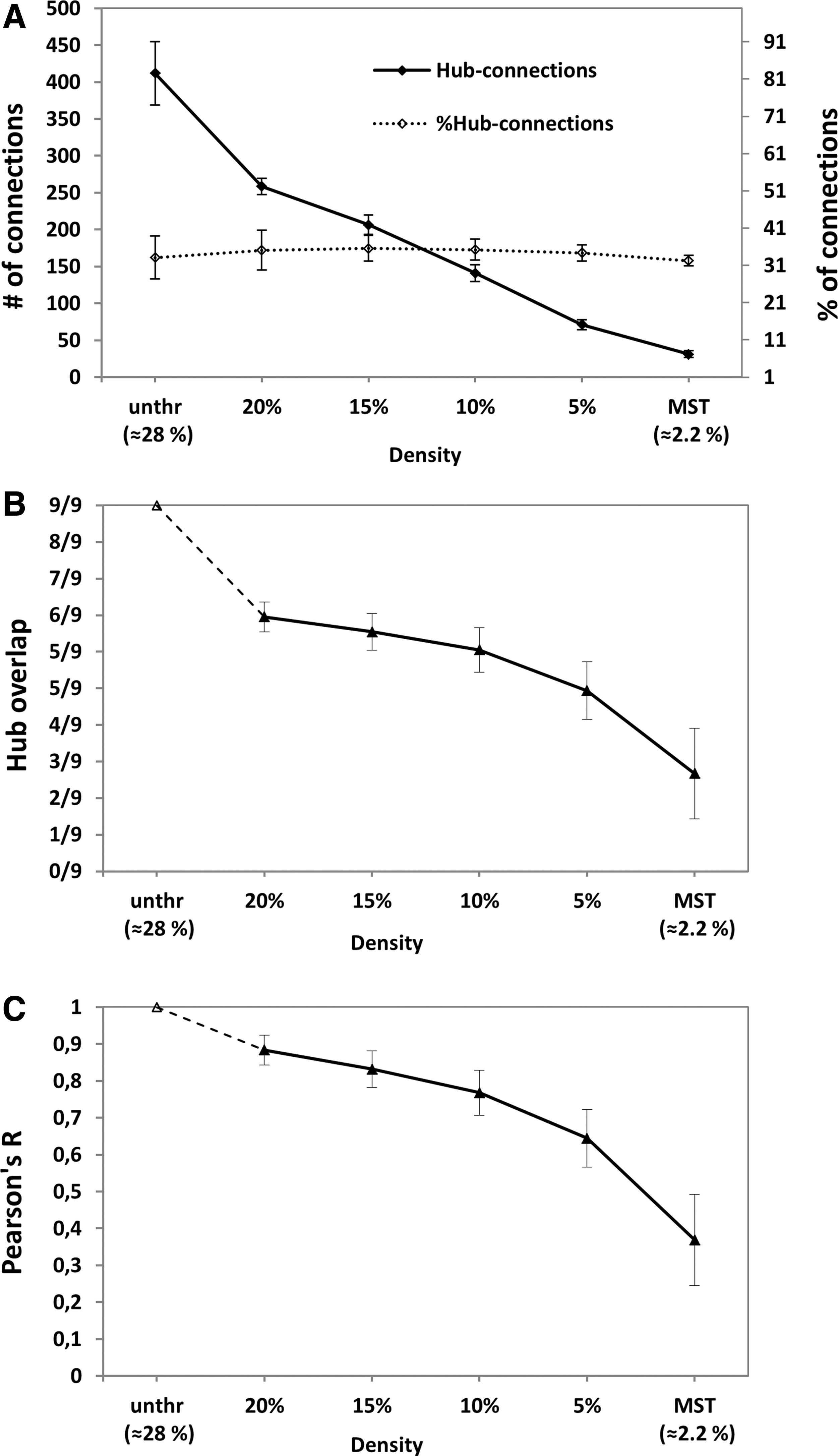
Effect of thresholding on hub connections and hub nodes. (A) Average number of hub connections retained in the network at each density level. This number is also represented as the percentage of all the edges retained in the network (dotted line, right y-axis). Error bars represent the SD. (B) Overlap between the hubs defined in the unthresholded network and the hubs defined in the thresholded networks (20%, 15%, 10%, 5% and MST). (C) Correlation between the nodal ranking of the unthresholded and nodal ranking of the thresholded networks (20%, 15%, 10%, 5% and MST). Note that each density is compared against the unthresholded network. Thus, the hub overlap and correlation coefficient for the unthresholded network are 9/9 and 1, respectively.

We found similar results when we compared the overall nodal ranking (i.e., the ranked betweenness centrality of all nodes) (Fig. 5C). There was a high correspondence in nodal ranking when a small proportion of edges was removed (r > 0.77 for densities ≥10%) and lower correspondence in nodal ranking when a larger proportion of edges was removed (r < 0.64 for densities ≤5%).

When we performed these analyses separately for patients and controls, fixed-density thresholding had a similar effect on the edge composition, hub location, and hub connections for both groups (Supplementary Figs. S2 and S3).

Effect of thresholding on the detection of SVD-related network impairments

In line with the previous literature (Heinen et al., 2018; Lawrence et al., 2014; Tuladhar et al., 2016), the global efficiency of the unthresholded FA-weighted network was lower in patients with SVD when compared with controls (Cohen's d = 0.97, p < 0.001; Fig. 6A). The between-group differences in global efficiency remained present after thresholding, irrespective of the network density (Fig. 6A). The largest effect size was observed at 15% density (Cohen's d = 1.09, interaction term density × group: p = 0.026).

FIG. 6.

Difference in weighted network measures between patients with SVD (red) and controls (blue) across different levels of network density. (A) FA-weighted global network efficiency. (B) Average FA-weighted strength of hub nodes. (C) Average FA-weighted strength of nonhub nodes. Hubs were defined in the control group; thus, the same nodes were considered hubs in both groups. *p < 0.001, Bonferroni corrected; age- and sex-adjusted effect sizes are given as Cohen's d. ^¥ p ≤ 0.026, density × group interaction. SVD, small vessel disease. Color images are available online.

The connectivity strength of hub nodes in the unthresholded network was lower in patients when compared with controls (Cohen's d = 1.11, p < 0.001, Fig. 6B). Again, the between-group difference remained significant after thresholding. The largest effect size in strength of hub nodes was observed at 10% density (Cohen's d = 1.18, interaction term density × group: p < 0.001).

Similarly, the largest effect size in strength of nonhub nodes was observed at 15% density (Cohen's d = 0.95, interaction term density × group: p < 0.001, Fig. 6C). At 10% and 5% densities, the group difference in strength of nonhub nodes was not significant and even reversed, indicating that the strength of nonhub nodes is less stable over thresholds.

Discussion

In this study, we investigated the impact of fixed-density thresholding on the basic architecture of structural brain networks and on the subsequent detection of network abnormalities in patients with SVD. Our results showed that fixed-density thresholding mainly removes edges composed of long streamlines but seemed independent of FA. The removed edges were not preferentially connected to hub or to nonhub nodes. As a result, more than half of the hubs and their original location, as well as the overall nodal ranking, were preserved when networks were thresholded to a density >10%. Importantly, our results also showed that the sensitivity to detect network abnormalities in patients with SVD is not affected by thresholding. Patients had a lower global efficiency and hub strength than controls when we compared their unthresholded networks. These between-group differences remained present in the thresholded networks, indicating that the disease effects are not removed by thresholding. Thresholding of brain networks in case-control studies remains a topic of intense debate (Stam, 2014). Some have argued that the difference in network density is partly a consequence of the disease, and enforcing a similar density would therefore lead to an elimination of disease effects. Here, we showed that disease effects were not removed by obtaining measures from brain networks with fixed densities.

Another argument against fixed-density thresholding in clinical network studies is that group differences may be artificially inflated. This effect is especially problematic when there is an initial group difference in the edge weights used for thresholding (van den Heuvel et al., 2017). Under these circumstances, more high-weight edges will be selected from the control networks than the patient networks to obtain the same network density, thereby increasing the between-group difference in network weight. This inflation of between-group differences is often a problem in functional network studies where the same measure of functional connectivity is used for thresholding as well as for calculation of network measures for group comparison. In our study however, the unthresholded networks of patients and controls had similar NOS weight distributions. Furthermore, the edge weight used to calculate graph metrics (i.e., FA) seemed independent of the weight used for thresholding (i.e., NOS). Therefore, this form of bias introduced by the difference in thresholding weight was not an issue.

We also found that a larger proportion of long-range connections was removed during thresholding, indicating that longer connections are often composed of low NOS (Roberts et al., 2017). A possible explanation for this bias is that long-range white matter pathways are inherently more difficult to tract because the likelihood of meeting the stopping criteria of the tractography algorithm (i.e., extreme fiber deviations or voxels with low FOD) is higher for long-range fibers (Jeurissen et al., 2017; Leopold et al., 2014). Understanding how the connection length is affected by thresholding is relevant because the role of long-range connections is a topic of interest in disease studies (Tuladhar et al., 2017), due to their contribution for global network signaling (van den Heuvel et al., 2012).

The edges removed during thresholding were not preferentially connected to hub nodes (or to nonhub nodes). In this way, the removal of edges seemed comparable with a “random network attack” (Mengiste et al., 2015). Brain networks are shown to be resilient to random attacks due to their hierarchical organization (Crossley et al., 2014). This resilience could also explain why the hub location and nodal ranking were largely unaffected when the networks were thresholded to densities ≥10%. These results suggest that a threshold between 10% and 15% can be applied without significantly damaging the backbone structure of brain networks. This is also supported by previous research that shows that brain networks preserve their small-world characteristics when they are thresholded to densities between 10% and 34% (Zhang et al., 2011).

Finally, we showed that the between-group differences in graph metrics are preserved after thresholding. In line with previous work, global efficiency and FA-weighted strength of hubs nodes in the unthresholded network were lower in patients with SVD than in controls (Lawrence et al., 2014; Reijmer et al., 2015). These group differences remained present after thresholding, which could be explained by the fact that there was no correlation between the NOS of the edges removed and their FA value. Thus, the FA weight used to calculate weighted graph metrics was not influenced by thresholding. Again, this shows the importance of using independent edge weights for thresholding and for the calculation of weighted graph metrics. Another explanation for the preservation of group differences is that thresholding had a similar impact on the network architecture of patients and controls. Thus, the computation of graph metrics was not affected differently for both groups. The only measure where the group differences were not maintained (for densities <10%) was the strength of nonhub nodes. Since these nodes have low degree to begin with, when the networks are thresholded to low densities, local graph metrics are calculated based on few connections (often only one), making the strength of nonhub nodes a less stable measure.

The fact that the largest effect sizes were observed at 10% and 15% densities suggests that fixed-density thresholding might improve the detection of between-group differences. It is possible that by applying moderate thresholds, the amount of spurious (false-positive) connections is reduced without significantly increasing the amount of false negatives (i.e., true connections removed during thresholding), which can improve the network specificity and sensitivity. Indeed, previous research indicates that reducing the amount of false positives in the network is more beneficial than safeguarding against the creation of new false negatives (Zalesky et al., 2016). These mid-range densities (10% and 15%) could represent the levels where this balance between false positives and false negatives is achieved. Thresholding beyond these levels would be detrimental to both the initial network architecture and the detection of between-group differences.

Strength of this study includes a standardized clinical MRI protocol with high-quality diffusion data from the TRACE-VCI cohort (Boomsma et al., 2017). Furthermore, we performed whole-brain tractography using CSD, which is known to have a better anatomical accuracy than the conventional diffusion tensor imaging approach (Jeurissen et al., 2013). Moreover, by incorporating the MST into the thresholded network, we ensured that the network did not become disconnected, avoiding differences in network structure due to disconnected nodes.

This study also has some limitations. Brain network reconstruction involves several choices in preprocessing steps, which could have influenced our results. The choice of parcellation scheme (Zalesky et al., 2010), tractography algorithm (Bastiani et al., 2012), and tractography parameters (e.g., FOD threshold, l-max, streamline deflection angle, etc.) can have a significant impact on the definition of nodes and edges as well as on the number of false positives and false negatives in the network. Consequently, these choices can influence the thresholding results and graph outcome measures obtained from these networks. Another limitation is that we did not consider the effect of thresholding on all network characteristics but only on network properties commonly investigated in network studies with SVD populations. Furthermore, we used the betweenness centrality as the only metric to characterize nodal ranking and define hub nodes. This may not fully describe the importance of a node for network integration and communication. Alternatively, a metric such as communicability (Andreotti et al., 2014a) could have provided a broader view of node importance. However, the interpretation of this metric is not straightforward and not established in clinical studies.

Future studies should examine the consequences of fixed-density thresholding on other network parameters and in other disease populations. Nevertheless, fixed-density thresholding may yield more reproducible networks, as suggested by repeatability studies (Andreotti et al., 2014b; Roine et al., 2018; Tsai et al., 2018). This can be beneficial in studies with a longitudinal design but further investigation is required.

Conclusion

We showed that moderate fixed-density thresholds (10% and 15% densities in this dataset) can be used to control for density effects in diffusion-based brain network studies. The present findings can help researchers make a well-informed choice when selecting an appropriate density threshold for future clinical studies.

Footnotes

Acknowledgments

Members of the Utrecht Vascular Cognitive Impairment (VCI) study group involved in this study (in alphabetical order by department): University Medical Center Utrecht, The Netherlands, Department of Neurology: E. van den Berg, J.M. Biesbroek, G.J. Biessels, M. Brundel, W.H. Bouvy, L.G. Exalto, C.J.M. Frijns, O. Groeneveld, S.M. Heringa, N. Kalsbeek, L.J. Kappelle, Y.D. Reijmer, J. Verwer; Department of Radiology/Image Sciences Institute: J. de Bresser, H.J. Kuijf, A. Leemans, P.R. Luijten, M.A. Viergever, K.L. Vincken, J.J.M. Zwanenburg; Department of Geriatrics: H.L. Koek; Hospital Diakonessenhuis Zeist, The Netherlands: M. Hamaker, R. Faaij, M. Pleizier, E. Vriens.

Author Disclosure Statement

No competing financial interests exist.

Funding Information

This work was supported by ZonMw, The Netherlands Organisation for Health Research and Development (Vidi Grant 91711384 and Vici Grant 91816616 to Geert Jan Biessels). Yael D. Reijmer receives funding from Alzheimer Nederland and ZonMw/Deltaplan Dementie (Grant #733050503) and a Young Talent Fellowship from the Brain Center Rudolf Magnus, University Medical Center Utrecht. Jil Meier is funded by a Weston Brain Institute Rapid Response grant and by the ALS Foundation Netherlands. The research of Alexander Leemans is supported by VIDI grant 639.072.411 from the Netherlands Organization for Scientific Research (NWO).

Supplementary Material

Supplementary Figure S1

Supplementary Figure S2

Supplementary Figure S3

References

Achard

, Bullmore

. 2007. Efficiency and cost of economical brain functional networks. PLoS Comput Biol, 3:0174–0183.

Achard

, Delon-Martin

, Vertes

, Renard

, Schenck

, Schneider

, et al. 2012. Hubs of brain functional networks are radically reorganized in comatose patients. Proc Natl Acad Sci U S A, 109:20608–20613.

Andreotti

, Abela

, Dierks

, Federspiel

, Melie-Garcia

, Jann

, et al. 2014a. Validation of network communicability metrics for the analysis of brain structural networks. PLoS One, 9:e115503.

Andreotti

, Jann

, Melie-Garcia

, Dierks

, Federspiel

, Giezendanner

. 2014b. Repeatability analysis of global and local metrics of brain structural networks. Brain Connect, 4:203–220.

Bassett

, Bullmore

. 2009. Human brain networks in health. Curr Opin Neurol, 10:324–336.

Bassett

, Bullmore

, Meyer-lindenberg

, Coppola

. 2009. Cognitive fitness of cost-efficient brain functional networks. Proc Natl Acad Sci U S A, 106:11747–11752.

Bastiani

, Shah

, Goebel

, Roebroeck

. 2012. Human cortical connectome reconstruction from diffusion weighted MRI: the effect of tractography algorithm. Neuroimage, 62:1732–1749.

Boomsma

JMF

, Exalto

, Barkhof

, van den Berg

, de Bresser

, Heinen

, et al. 2017. Vascular cognitive impairment in a memory clinic population: rationale and design of the “Utrecht-Amsterdam Clinical Features and Prognosis in Vascular Cognitive Impairment” (TRACE-VCI) study. JMIR Res Protoc, 6:e60.

Crossley

, Mechelli

, Scott

, Carletti

, Fox

, Mcguire

, Bullmore

. 2014. The hubs of the human connectome are generally implicated in the anatomy of brain disorders. Brain, 137:2382–2395.

10.

Daianu

, Jahanshad

, Nir

, Jack

, Weiner

, Bernstein

, Thompson

. 2015. Rich club analysis in the Alzheimer's disease connectome reveals a relatively undisturbed structural core network. Hum Brain Mapp, 36:3087–3103.

11.

Daianu

, Mezher

, Mendez

, Jahanshad

, Jimenez

, Thompson

. 2016. Disrupted rich club network in behavioral variant frontotemporal dementia and early-onset Alzheimer's disease. Hum Brain Mapp, 37:868–883.

12.

Drakesmith

, Caeyenberghs

, Dutt

, Lewis

, David

, Jones

. 2015. Overcoming the effects of false positives and threshold bias in graph theoretical analyses of neuroimaging data. Neuroimage, 118:313–333.

13.

Fagerholm

, Hellyer

, Scott

, Leech

, Sharp

. 2015. Disconnection of network hubs and cognitive impairment after traumatic brain injury. Brain, 138:1696–1709.

14.

Ferro

, Heinen

, De Brito Robalo

, Kuijf

, Biessels

, Reijmer

. 2019. Cortical microinfarcts and white matter connectivity in memory clinic patients. Front Neurol, 10:571.

15.

Garrison

, Scheinost

, Finn

, Shen

, Constable

. 2015. The (in)stability of functional brain network measures across thresholds. Neuroimage, 118:651–661.

16.

Hagmann

, Cammoun

, Gigandet

, Meuli

, Honey

, Van Wedeen

, Sporns

. 2008. Mapping the structural core of human cerebral cortex. PLoS Biol, 6:1479–1493.

17.

Hein

KHM

, Neher

, Christophe

, Alexandre

. 2016. Tractography-based connectomes are dominated by false-positive connections. BioRxiv. 1–23. DOI: 10.1101/084137.

18.

Heinen

, Vlegels

, de Bresser

, Leemans

, Biessels

, Reijmer

. 2018. The cumulative effect of small vessel disease lesions is reflected in structural brain networks of memory clinic patients. Neuroimage, 19:963–969.

19.

Jeurissen

, Descoteaux

, Mori

, Leemans

. 2017. Diffusion MRI fiber tractography of the brain. NMR Biomed, 32:e3785.

20.

Jeurissen

, Leemans

, Jones

, Tournier

, Sijbers

. 2011. Probabilistic fiber tracking using the residual bootstrap with constrained spherical deconvolution. Hum Brain Mapp, 32:461–479.

21.

Jeurissen

, Leemans

, Tournier

, Jones

, Sijbers

. 2013. Investigating the prevalence of complex fiber configurations in white matter tissue with diffusion magnetic resonance imaging. Hum Brain Mapp, 34:2747–2766.

22.

Jones

DK.

2008. Studying connections in the living human brain with diffusion MRI. Cortex, 44:936–952.

23.

Kruskal

JB.

1956. On the shortest spanning subtree of a graph and the traveling salesman problem. Proc Am Math Soc, 7:48.

24.

Lawrence

, Chung

, Morris

, Markus

, Barrick

. 2014. Structural network efficiency is associated with cognitive impairment in small-vessel disease. Neurology, 83:304–311.

25.

Leemans

, Jeruissen

, Sijbers

, Jones

. 2009. ExploreDTI: a graphical toolbox for processing, analyzing, and visualizing diffusion MR data. Proc Int Soc Magn Reson Med, 245:3537.

26.

Leemans

, Jones

. 2009. The B-matrix must be rotated when correcting for subject motion in DTI data. Magn Reson Med, 61:1336–1349.

27.

Leopold

, Modi

, Thomas

, Irfanoglu

, Saleem

, Ye

, Pierpaoli

. 2014. Anatomical accuracy of brain connections derived from diffusion MRI tractography is inherently limited. Proc Natl Acad Sci U S A, 111:16574–16579.

28.

Liu

, Li

, Pan

, Lan

, Zheng

, Wu

, Wang

. 2017. Complex brain network analysis and its applications to brain disorders: a survey. Complex, 2017:1–27. DOI: 10.1155/2017/8362741.

29.

Mårtensson

, Pereira

, Mecocci

, Vellas

, Tsolaki

, Kłoszewska

, et al. 2018. Stability of graph theoretical measures in structural brain networks in Alzheimer's disease. Sci Rep, 8:1–15.

30.

Mengiste

, Aertsen

, Kumar

. 2015. Effect of edge pruning on structural controllability and observability of complex networks. Sci Rep, 5:1–14.

31.

Odish

OFF

, Caeyenberghs

, Hosseini

, Van Den Bogaard

SJA

, Roos

RAC

, Leemans

. 2015. Dynamics of the connectome in Huntington's disease: a longitudinal diffusion MRI study. Neuroimage, 9:32–43.

32.

Pandit

, Expert

, Lambiotte

, Bonnelle

, Leech

, Turkheimer

, Sharp

. 2013. Traumatic brain injury impairs small-world topology. Neurology, 80:1826–1833.

33.

, Meesters

, Nicolay

, ter Haar Romeny

, Ossenblok

. 2015. The influence of construction methodology on structural brain network measures: a review. J Neurosci Methods, 253:170–182.

34.

Reijmer

, Fotiadis

, Martinez-Ramirez

, Salat

, Schultz

, Shoamanesh

, et al. 2015. Structural network alterations and neurological dysfunction in cerebral amyloid angiopathy. Brain, 138:179–188.

35.

Roberts

, Perry

, Roberts

, Mitchell

, Breakspear

. 2017. Consistency-based thresholding of the human connectome. Neuroimage, 145:118–129.

36.

Roine

, Aelterman

, Sijbers

, Jeurissen

, Philips

, Leemans

, Perrone

. 2018. Reproducibility and intercorrelation of graph theoretical measures in structural brain connectivity networks. Med Image Anal, 52:56–67.

37.

Rubinov

, Sporns

. 2010. Complex network measures of brain connectivity: uses and interpretations. Neuroimage, 52:1059–1069.

38.

Sarwar

, Ramamohanarao

, Zalesky

. 2019. Mapping connectomes with diffusion MRI: deterministic or probabilistic tractography?. Magn Reson Med, 81:1368–1384.

39.

Sporns

, Tononi

, Kötter

. 2005. The human connectome: a structural description of the human brain. PLoS Comput Biol, 1:0245–0251.

40.

Stam

CJ.

2014. Modern network science of neurological disorders. Nat Rev Neurosci, 15:683–695.

41.

Tax

CMW

, Otte

, Viergever

, Dijkhuizen

, Leemans

. 2015. REKINDLE: Robust Extraction of Kurtosis INDices with linear estimation. Magn Reson Med, 73:794–808.

42.

Telesford

, Simpson

, Burdette

, Hayasaka

, Laurienti

. 2011. The brain as a complex system: using network science as a tool for understanding the brain. Brain Connect, 1:295–308.

43.

Tewarie

, van Dellen

, Hillebrand

, Stam

C.J

. 2015. The minimum spanning tree: an unbiased method for brain network analysis. Neuroimage, 104:177–188.

44.

Tsai

SY.

2018. Reproducibility of structural brain connectivity and network metrics using probabilistic diffusion tractography. Sci Rep, 8:1–12.

45.

Tuladhar

, Lawrence

, Norris

, Barrick

, Markus

, de Leeuw

. 2017. Disruption of rich club organisation in cerebral small vessel disease. Hum Brain Mapp, 38:1751–1766.

46.

Tuladhar

, van Dijk

, Zwiers

, van Norden

AGW

, de Laat

, Shumskaya

, et al. 2016. Structural network connectivity and cognition in cerebral small vessel disease. Hum Brain Mapp, 37:300–310.

47.

Tzourio-Mazoyer

, Landeau

, Papathanassiou

, Crivello

, Etard

, Delcroix

, et al. 2002. Automated anatomical labeling of activations in SPM using a macroscopic anatomical parcellation of the MNI MRI single-subject brain. Neuroimage, 15:273–289.

48.

van Dellen

, Sommer

, Bohlken

, Tewarie

, Draaisma

, Zalesky

, et al. 2018. Minimum spanning tree analysis of the human connectome. Hum Brain Mapp, 39:2455–2471.

49.

Van Den Berg

, Reijmer

, De Bresser

, Kessels

RPC

, Kappelle

, Biessels

. 2010. A 4 year follow-up study of cognitive functioning in patients with type 2 diabetes mellitus. Diabetologia, 53:58–65.

50.

van den Heuvel

, de Lange

, Zalesky

, Seguin

, Yeo

BTT

, Schmidt

. 2017. Proportional thresholding in resting-state fMRI functional connectivity networks and consequences for patient-control connectome studies: issues and recommendations. Neuroimage, 152:437–449.

51.

van den Heuvel

, Kahn

, Goni

, Sporns

. 2012. High-cost, high-capacity backbone for global brain communication. Proc Natl Acad Sci U S A, 109:11372–11377.

52.

van den Heuvel

, Sporns

. 2011. Rich-club organization of the human connectome. J Neurosci, 31:15775–15786.

53.

van den Heuvel

, Sporns

. 2013. Network hubs in the human brain. Trends Cogn Sci, 17:683–696.

54.

van den Heuvel

, Stam

, Boersma

, Hulshoff Pol

. 2008. Small-world and scale-free organization of voxel-based resting-state functional connectivity in the human brain. Neuroimage, 15:528–539.

55.

van Wijk

BCM

, Stam

, Daffertshofer

. 2010. Comparing brain networks of different size and connectivity density using graph theory. PLoS One 5:. 13701.

56.

Váša

, Bullmore

, Patel

. 2018. Probabilistic thresholding of functional connectomes: application to schizophrenia. Neuroimage, 172:326–340.

57.

Veraart

, Sijbers

, Sunaert

, Leemans

, Jeurissen

. 2013. Weighted linear least squares estimation of diffusion MRI parameters: strengths, limitations, and pitfalls. Neuroimage, 81:335–346.

58.

Vos

, Tax

CMW

, Luijten

, Ourselin

, Leemans

, Froeling

. 2017. The importance of correcting for signal drift in diffusion MRI. Magn Reson Med, 77:285–299.

59.

Wardlaw

, Smith

, Biessels

, Cordonnier

, Fazekas

, Frayne

, et al. 2013. Neuroimaging standards for research into small vessel disease and its contribution to ageing and neurodegeneration. Lancet Neurol, 12:822–838.

60.

Zalesky

, Fornito

, Cocchi

, Gollo

, van den Heuvel

, Breakspear

. 2016. Connectome sensitivity or specificity: which is more important?. Neuroimage, 142:407–420.

61.

Zalesky

, Fornito

, Harding

, Cocchi

, Yücel

, Pantelis

, Bullmore

. 2010. Whole-brain anatomical networks: does the choice of nodes matter?. Neuroimage, 50:970–983.

62.

Zhang

, Wang

, Wu

, Kuang

, Huang

, He

, Gong

. 2011. Disrupted brain connectivity networks in drug-naive, first-episode major depressive disorder. Biol Psychiatry, 70:334–342.

Supplementary Material

Please find the following supplemental material available below.

For Open Access articles published under a Creative Commons License, all supplemental material carries the same license as the article it is associated with.

For non-Open Access articles published, all supplemental material carries a non-exclusive license, and permission requests for re-use of supplemental material or any part of supplemental material shall be sent directly to the copyright owner as specified in the copyright notice associated with the article.

0.00 MB

0.15 MB

0.18 MB

0.15 MB