BrainNET: Inference of Brain Network Topology Using Machine Learning

Abstract

Background:

To develop a new functional magnetic resonance image (fMRI) network inference method, BrainNET, that utilizes an efficient machine learning algorithm to quantify contributions of various regions of interests (ROIs) in the brain to a specific ROI.

Methods:

BrainNET is based on extremely randomized trees to estimate network topology from fMRI data and modified to generate an adjacency matrix representing brain network topology, without reliance on arbitrary thresholds. Open-source simulated fMRI data of 50 subjects in 28 different simulations under various confounding conditions with known ground truth were used to validate the method. Performance was compared with correlation and partial correlation (PC). The real-world performance was then evaluated in a publicly available attention-deficit/hyperactivity disorder (ADHD) data set, including 134 typically developing children (mean age: 12.03, males: 83), 75 ADHD inattentive (mean age: 11.46, males: 56), and 93 ADHD combined (mean age: 11.86, males: 77) subjects. Network topologies in ADHD were inferred using BrainNET, correlation, and PC. Graph metrics were extracted to determine differences between the ADHD groups.

Results:

BrainNET demonstrated excellent performance across all simulations and varying confounders in identifying the true presence of connections. In the ADHD data set, BrainNET was able to identify significant changes (p < 0.05) in graph metrics between groups. No significant changes in graph metrics between ADHD groups were identified using correlation and PC.

Conclusion:

We describe BrainNET, a new network inference method to estimate fMRI connectivity that was adapted from gene regulatory methods. BrainNET out-performed Pearson correlation and PC in fMRI simulation data and real-world ADHD data. BrainNET can be used independently or combined with other existing methods as a useful tool to understand network changes and to determine the true network topology of the brain under various conditions and disease states.

Impact statement

Developed a new functional magnetic resonance image (fMRI) network inference method named as BrainNET using machine learning.

BrainNET out-performed Pearson correlation and partial correlation in fMRI simulation data and real-world attention-deficit/hyperactivity disorder data.

BrainNET does not need to be pretrained and can be applied to infer fMRI network topology independently on individual subjects and for varying number of nodes.

Introduction

The brain is a complex interconnected network that balances segregation and specialization of function with strong integration between regions, resulting in complex and precisely coordinated dynamics across multiple spatiotemporal scales (Sporns, 2018). Connectomics and graph theory offer powerful tools for mapping, tracking, and predicting patterns of disease in brain disorders through modeling brain function as complex networks (Fornito et al., 2015). Studying brain network organization provides insight in understanding global network connectivity abnormalities in neurological and psychiatric disorders (Avena-Koenigsberger et al., 2018). Several studies suggest that pathology accumulates in highly connected hub areas of the brain (Buckner et al., 2009; Crossley et al., 2014) and that cognitive sequelae are closely related to the connection topology of the affected regions (Warren et al., 2014). An understanding of network topology may allow prediction of expected levels of impairment, determination of recovery following an insult, and selection of individually tailored interventions for maximizing therapeutic success (Fornito et al., 2016). A large number of network inference methods are being used to model brain network topology with varying degrees of validation. A recent study (Smith et al., 2011) evaluated some of the most common methods, including correlation, partial correlation (PC), and Bayes NET, to infer network topology using simulated resting-state functional magnetic resonance image (rs-fMRI) data with known ground truth and found that performance can vary widely under different conditions.

Development of statistical techniques for valid inferences on disease-specific group differences in brain network topology is an active area of research (Kim et al., 2015, 2019). Machine learning methods have been used in neuroimaging for disease diagnosis and anatomic segmentation (Murugesan et al., 2018; Zaharchuk et al., 2018). Brain Network Construction and Classification (BrainNetClass) and GraphVar toolboxes provide a full pipeline from network construction to classification. BrainNetClass comprises various fMRI network inference methods such as correlation, PC, and higher order functional connectivity for brain network inference followed by feature extraction for machine learning model development and testing (Waller et al., 2018; Zhou et al., 2020). Very few studies have attempted to apply machine learning methods on direct time series of fMRI to infer brain networks (O'Neill et al., 2017; Pellegrini et al., 2018; Williams and Henson, 2018; Zaharchuk et al., 2018). Recent work in machine learning approaches for inference of gene regulatory networks (GRN) has demonstrated excellent performance (Camacho et al., 2018; Finkle et al., 2018; Turki et al., 2016). Interestingly, these same approaches to GRNs can be used to infer brain networks. In this study, we describe a new network inference method called BrainNET, inspired by machine learning methods used to infer GRN (Irrthum et al., 2010).

Yan et al. (2018) devised a bidirectional long short-term memory (LSTM) deep learning network (Full-BiLSTM) to effectively learn the periodic fMRI brain status changes using both past and future information for each brief time segment. They then fused them to form the final output by taking a dynamic functional connectivity matrix calculated using the sliding window approach as input (Yan et al., 2018). Higher order functional connectivity was developed by Chen et al. (2016) by taking dynamic relationships between the brain regions to infer network topology. Yu et al. (2017) proposed a novel method using connectivity weighted sparse representation to construct optimal brain functional networks from rs-fMRI data. The method has taken advantage of both Pearson's correlation and sparse representations, which are the two most commonly used brain network modeling approaches. This ensures the construction of more biologically meaningful brain networks by a unified framework that integrates connectivity strength, group structure, and sparsity. Yu et al. (2017) used l1-norm regularized linear regression or sparse representation, which learns a linear relationship, while BrainNET considers the nonlinear relationships. The abovementioned methods, including BrainNetClass and GraphVar, focus on using machine learning methods for computer-aided diagnosis by predicting the cognitive metrics or classifying a group of the subjects, whereas BrainNET uses machine learning for inferring the networks directly.

Validation of BrainNET was performed using fMRI simulations with known ground, as well as in real-world attention-deficit/hyperactivity disorder (ADHD) fMRI data sets. In this study, publicly available resting-state fMRI simulated data (Smith et al., 2011) were used to validate BrainNET's ability to infer networks. The real-world performance of BrainNET was then evaluated in a publicly available data set of ADHD. ADHD is one of the most common neurodevelopmental disorders in children with significant socioeconomic and psychological effects (Hilger and Fiebach, 2019; Lin et al., 2014). It can be difficult to diagnose due to the overlapping nature of symptoms, with resultant diagnostic errors and overprescribing of medications due to misdiagnosis (Saeed, 2018). ADHD has widespread but often subtle alterations in multiple brain regions affecting brain function (Cortese et al., 2012; Sidlauskaite et al., 2015). Neuro Bureau, a collaborative neuroscience forum, has released fully processed open-source fMRI data “ADHD-200 preprocessed” from several sites (Bellec et al., 2017; Milham et al., 2012) providing an ideal data set to test the BrainNET model and compare its performance with standard correlation and PC, the most widely used methodology to infer brain networks using fMRI data.

Materials and Methods

Data sets

MRI simulation data

Open-source rs-fMRI simulation data representing brain dynamics were used to validate the BrainNET model (Smith et al., 2011). The data were simulated based upon the dynamic causal modeling fMRI forward model, which uses the nonlinear balloon model for vascular dynamics, in combination with a neural network model (Smith et al., 2011). The open-source data set has 28 simulations, each including simulated data for 50 subjects with a varying number of nodes and several confounders (e.g., shared input between the nodes, varying fMRI session lengths, noise, cyclic connections, and hemodynamic lag variability changes). Additional details on the simulations can be found in the original study (Supplementary Table S1) (Smith et al., 2011).

ADHD data

Preprocessed rs-fMRI data were obtained from the ADHD-200 database (http://fcon1000.projects.nitrc.org/indi/adhd200). IRB approval is not required for deidentified data received from an open repository. Seven different sites contributed to the ADHD-200 database for 776 rs-fMRI data acquisitions. The data were preprocessed using the Athena pipeline and were provided in 3D NifTI format. Additional information on the Athena pipeline and “ADHD 200 preprocessed” data are detailed by Bellec et al. (2017).

In our study, subjects identified with “no naive medication” status, or questionable quality on rs-fMRI data was excluded. The remaining subjects were age-matched between the groups resulting in 135 typically developing children (TDC) (mean age: 12.00, males: 83), 75 ADHD inattentive (ADHD-I) (mean age: 11.46, males: 56), and 93 ADHD combined (ADHD-C) (mean age: 11.86, males: 77) subjects. Mean time series from 116 regions of interests (ROIs) in the automated anatomic atlas (AAL) atlas (Tzourio-Mazoyer et al., 2002) were extracted using the NILEARN package (Abraham et al., 2014).

BrainNET model development

The objective of BrainNET is to infer the connectivity from fMRI data as a network with N different nodes in the brain (i.e., ROIs), where edges between the nodes represent the true functional connectivity between nodes. At each node, there are measurements from m time points $X = \{x_{1}, x_{2}, x_{3}, x_{4}, \dots ., x_{N}\},$ where x_i is the vector representation of m time points measured as

Our method assumes that fMRI measurement of BOLD (blood oxygen level dependent) activation at each node is a function of each of the other nodes' activation with additional random noise.

For the jth node with m time points, a vector can be defined denoting all nodes except the jth node as $x_{- j} = (x_{1}, x_{2}, x_{j - 1}, x_{j + 1}, \dots . ., x_{N}),$ then the measurements at the jth node can be represented as a function of other nodes as

$x_{j} = f_{j} (x_{- j}) + ɛ_{j}$

where ɛ_j is random noise specific to each node_j. We further assume that function ƒ_j () only exploits the data of nodes in x_−j that are connected to node_j. The function ƒ_j () can be solved in various ways in the context of machine learning. Since the nature of the relationship between different ROIs in the brain is unknown and expected to be nonlinear (Stam and Reijneveld, 2007), we choose a tree-based ensemble method as it works well with a large number of features with nonlinear relationships and is computationally efficient. We utilized extremely randomized trees (ERT), an ensemble algorithm similar to random forest, which aggregates several weak learners to form a robust model. ERT uses a random subset of predictors to select divergences in a tree node and then selects the “best split” from this limited number of choices (Praagman, 1985). Finally, outputs from individual trees are averaged to obtain the best overall model (Petralia et al., 2015). BrainNET infers a network with N different nodes by dividing the problem into N different subproblems, and solving the function ƒ_j () for each node independently as illustrated in Figure 1. The steps are listed below:

FIG. 1.

Schematic overview of the BrainNET model. For N nodes in fMRI data (X), each node will have m time points such that $X = \{x_{1}, x_{2}, x_{3}, x_{4}, \dots ., x_{N}\},$ where x_i is the vector representation of m time points measured as . Each node's time series (x_n ) is predicted from all other nodes time series (x_-n ) using the ERT regressor. Node importance of each node for predicting the target node is extracted and populated in the importance matrix. The average of the upper and lower triangle of the matrix is thresholded at (1/Num of Nodes) to obtain an adjacency matrix representing the network topology. ERT, extremely randomized trees; fMRI, functional magnetic resonance images. Color images are available online.

For j = 1 to N nodes

Fit the ERT regressor with all the node data, except the jth node, to find the function f_j that minimizes the following mean squared error:

$1 ∕ m \sum_{k = 1}^{m} {(x_{j} - f_{j} (x_{- j}))}^{2}$

Extract the weight of each node to predict node j,

$W (j, n) = \{\begin{matrix} w_{n} i f n \neq j \\ 0 i f n = j \end{matrix}$

where w_n is the weight of node to predict node j and n = 1 to N.

Append the weight values to the importance matrix.

The importance score for each node (Node_j) to predict (Node_i) is defined as the total decrease in impurity due to splitting the samples based on Node_j (Praagman, 1985). The GINI index is used here as the measure of impurity. Let “S” denote a node split in the tree ensemble and let (S_L, S_R) denote its left and right children nodes. Then, the decrease in impurity ΔImpurity(S) from node split “S” based on Node_j to predict Node_i is defined as follows:

$\begin{matrix} Δ I m p u r i t y (S_{i j}) & = I m p u r i t y (S) - (N_{L} ∕ N_{P}) * I m p u r i t y (S_{L}) \\ - (N_{R} ∕ N_{P}) * I m p u r i t y (S_{R}) \end{matrix}$

where S_L and S_R are left and right splits and N_P, N_L, N_R are number of samples reaching parent, left, and right nodes, respectively. Let be the number of ensembles, which uses ROI_j for splitting trees. Then, the importance score for Node_j for predicting Node_i is calculated as the average of node impurities across all trees, that is, importance of ROI_ji

where T is the number of trees in the ensemble.

Importance values extracted using a typical random forest model can be biased in the presence of two or more correlated features since the model will randomly assign importance to any one of the equally important features without any preference (Strobl et al., 2007). This problem is avoided by using the ERT regressor. The comparison between ERT, random forest, and baseline LASSO in inferring network topology with the simulation data is provided in Supplementary Figure S1 and Supplementary Table S2.

The importance of each node to predict all other node time series is extracted from the model and an N × N (where N is the number of nodes) importance matrix is generated with the diagonal equal to zero. Each row of the importance matrix represents normalized weights of each node in predicting the target node. The extracted adjacency matrix is affected in two ways. First, due to the row-wise normalization, the upper triangular values of the importance matrix are not same as the lower triangle values. We therefore take the average of the upper triangle and the lower triangle of the matrix to make it symmetric to determine the presence of connection between the nodes. This procedure does not allow directionality of the connections to be determined. The comparison between ERT, random forest, and baseline LASSO in inferring network topology with the lower and upper triangle, averaged (symmetrized) and nonaveraged (nonsymmetrized), is provided in Supplementary Figure S1 Second, again because of the row-wise normalization, the sum of each row in the importance matrix is one. Since the importance values are normalized with respect to number of nodes in the analysis, we used a threshold that is inversely proportional to the number of nodes (i.e., threshold = 1/number of nodes) in the network to produce a final adjacency matrix representing the network topology. The selection of threshold is not based on statistical theory and it is not made to keep the false positive rate below a nominal level, but it results in a dynamically changing threshold based on the number of nodes in the network.

Analysis

Evaluation of inference methods on simulation data

Evaluation of inference methods on simulation data using c-sensitivity

The network topology was inferred using BrainNET, correlation, and PC. The network topology inferred by correlation and PC method may vary drastically based on the values used to threshold connectivity matrix. Hence, we evaluated the ability of the inference methods based on BrainNET, correlation, and PC to detect the presence of connection between the nodes in terms of c-sensitivity. C-sensitivity quantifies how well the true positives (TPs) are separated from the false positives (FPs) by measuring the fraction of TPs that are estimated with a higher connection strength than the 95th percentile of the FP distribution. C-sensitivity is a measure of success in separating true connections from FP connections and it is calculated by counting the number of TPs above the 95th percentile of FPs and then divided by the total number of TPs (Smith et al., 2011).

Effects of simulation parameters such as TR (repetition time), number of nodes, noise, hemodynamic response function standard deviation, shared inputs, bad ROIs, backward, strong, and cyclic connections, and strong inputs on c-sensitivity of the inference methods were evaluated using the mixed-effects model with a random effect for the simulation to control for the effect of the specific generating model. The mixed-effects models were fit across subjects under different simulations to analyze the effects of simulation parameters on c-sensitivity of the inference methods. The parameter estimates from each regression were then summarized across subjects in terms of their effect size (Smith et al., 2011).

Evaluation of inference methods on simulation data using threshold

Thresholding can be applied to suppress spurious connections that may arise from measurement noise and imperfect connectome reconstruction techniques and to potentially improve statistical power and interpretability (Fornito et al., 2016). However, based on the threshold value, the connection density of each network inferred by correlation and PC may vary from network to network after the threshold has been applied. Using a less stringent lower threshold value results in higher FP values (lower sensitivity) and a more stringent threshold results in higher false negatives (lower specificity). This can lead to wide variability in computed graph metrics, as they are typically susceptible to the number of edges in a graph. Identifying an appropriate threshold to infer the underlying brain network topology is critical.

Hence, we evaluated the specificity, sensitivity, and accuracy of correlation and PC under varying thresholds. The results show that the network topology inferred using correlation and PC method may vary drastically based on the threshold values (Fig. 2). An optimum threshold for correlation methods can be very difficult to find in real-life experimental data. However, given the ground truth for the simulation data, we calculated the optimum threshold values for the correlation methods and compared their performance at optimum threshold with BrainNET. The optimal thresholds are defined where the correlation and PC methods performed with the best sensitivity and accuracy. It is important to note that BrainNET is not optimized on these simulation data, and the threshold is based on the number of nodes inferred in the network. Specificity, sensitivity, and accuracy of correlation and PC at threshold values of 30% (Corr₃₀, PC₃₀) and optimum (Corr_opt, PC_opt) values are estimated and compared with BrainNET. We further evaluated the specificity, sensitivity, and accuracy of the Corr_opt and PC_opt with BrainNET for each simulation. Similar to the c-sensitivity, we calculated the effect of simulation parameters on the sensitivity and specificity of BrainNET, Corr_opt, and PC_opt.

FIG. 2.

Sensitivity analysis for correlation and PC. Average sensitivity (true-positive rate) and specificity across 28 simulations for the correlation and PC methods are plotted as a function of threshold ranging between 0% and 100%. Optimum threshold is found using simulation ground truth at 20% and 16% for correlation and PC, respectively. PC, partial correlation. Color images are available online.

Evaluation of inference methods on ADHD data

BrainNET, correlation, and PC were applied to the real-world ADHD data to evaluate whole-brain network changes in ADHD subtypes (i.e., ADHD-C, ADHD-I) compared with TDC. Mean time series from 116 ROIs in the AAL atlas (Tzourio-Mazoyer et al., 2002) were extracted using the NILEARN package (Abraham et al., 2014). The BrainNET model was applied to extract an importance matrix for each subject. The importance matrix was then thresholded at 1/number of nodes (e.g., 1/116 for the AAL atlas regions) to obtain an adjacency matrix for each subject (BN). Functional network connectivity was calculated between the 116 ROIs using correlation and PC. The connectivity matrices are thresholded at a threshold of 20% and 30% (Corr₂₀, Corr₃₀, PC₂₀, and PC₃₀) (no optimum threshold for real-world experimental data). Graph theoretic metrics were extracted using each of these methods for each group. Network differences between the three groups TDC, ADHD-I, and ADHD-A were then computed using t-tests on the graph metrics. Site effects and effects of age and handedness were removed using the ComBat multisite harmonization method (Yamashita et al., 2019), an effective harmonization technique that both removes unwanted variation associated with the site and preserves biological associations in the data (Fortin et al., 2018).

Graph metrics

Graph theoretical metrics representing global and local characteristics of network topology were used to compare between the groups in the ADHD data set. The GRETNA MATLAB toolbox (v2.0, https://www.nitrc.org/projects/gretna) was used to extract additional graph theoretical metrics, including shortest path length, global network efficiency, and betweenness centrality (BC) (Wang et al., 2015). The NetworkX package in python was used to extract the graph theoretical metrics, including density, average clustering coefficient, and characteristic path length (CPL) (Hagberg et al., 2013). Two-sample t-tests between groups were performed using the GRETNA toolbox. Bonferroni multiple comparison correction was applied with statistical significance set at p < 0.05.

Node metrics

The nodal shortest path length (NSPL) is defined as the shortest mean distance from a particular node to all other nodes in the graph. Shorter NSPL represents greater integration (Sporns, 2018). The BC measures a node's influence in information flow between all other nodes (Wang et al., 2010). BC quantifies the influence of a node and is defined as the number of shortest paths passing through it.

Global metrics

Network efficiency is a more biologically relevant measure representing the ability of the network to transmit information globally and locally. Networks with high efficiency, both globally and locally, are said to be economic small-world networks (Achard and Bullmore, 2007). The density of the graph is defined as the ratio of number of connections in the network to the number of possible connections in the network. Average clustering is the fraction of a node's neighbors that are neighbors of each other. The clustering coefficient of a graph is the average clustering coefficient over all nodes in the network. Networks with high clustering coefficient are considered locally efficient networks. CPL is the average shortest path length between nodes in the graph, with a minimum number of edges that must be traversed to get from one node to another. CPL indicates how easily information can be transferred across the network (Sporns, 2018).

Experimental Results

Simulation data

Evaluation of inference methods using c-sensitivity

BrainNET performed significantly better than correlation (p < 0.001) and equivalent to PC (p > 0.05) methods with c-sensitivity of 79.53%, 59.82%, and 75.75%, respectively, across 28 simulations (Fig. 3A and Supplementary Table S3).

FIG. 3.

C-sensitivity. Boxplots of c-sensitivity for BrainNET, correlation, and PC (left). The effects of different simulation parameters on the c-sensitivity, sensitivity, and specificity of inference methods using mixed-effects model. The color bar represents the effect size of each simulation parameter on the c-sensitivity, sensitivity, and specificity of inference methods (right). Color images are available online.

The study on the effect of simulation parameters on the c-sensitivity of inference methods showed that increasing the number of nodes and session duration does not have much effect on any of the inference methods (Fig. 3B). Having shared inputs between the nodes affected the correlation and PC method more drastically than the BrainNET method. Selection of bad ROIs with mixed time series between them affected all the inference methods negatively, however, selection of bad ROIs with randomly random time series mixed between them did not affect the inference methods drastically. The presence of cyclic and backward connection between the nodes affected the correlation and PC methods but not BrainNET. The presence of only one strong input affected the performance of the BrainNET method but not the other methods. In summary, BrainNET performance was robust under various confounding factors but prone to selection of inaccurate ROIs with mixed time series between them and networks with only one strong input. Both PC and correlation methods were affected by shared inputs between the nodes, selection of inaccurate ROIs, and backward, cyclic, and stationary/nonstationary connections between the nodes.

Evaluation of inference methods using threshold

The accuracy, sensitivity, and specificity for each method across all 28 simulated data sets were estimated at thresholds of 30% and at optimum value for correlation and PC, and at a threshold of 1/number of nodes for BrainNET (Fig. 4). BrainNET achieved higher accuracy and specificity at a threshold of 30% compared with the Corr₃₀ and PC₃₀ method, as shown in Figure 4. PC_opt achieved a slightly higher accuracy than BrainNET across 28 simulations, but no significant difference in terms of specificity and accuracy even at its optimum (p > 0.05) (Fig. 5). As expected, the specificity and sensitivity of correlation and PC methods vary with threshold and it will be difficult to find an optimum threshold in a real-life data set. BrainNET showed more robust performance with little variance across the simulation compared with other methods.

FIG. 4.

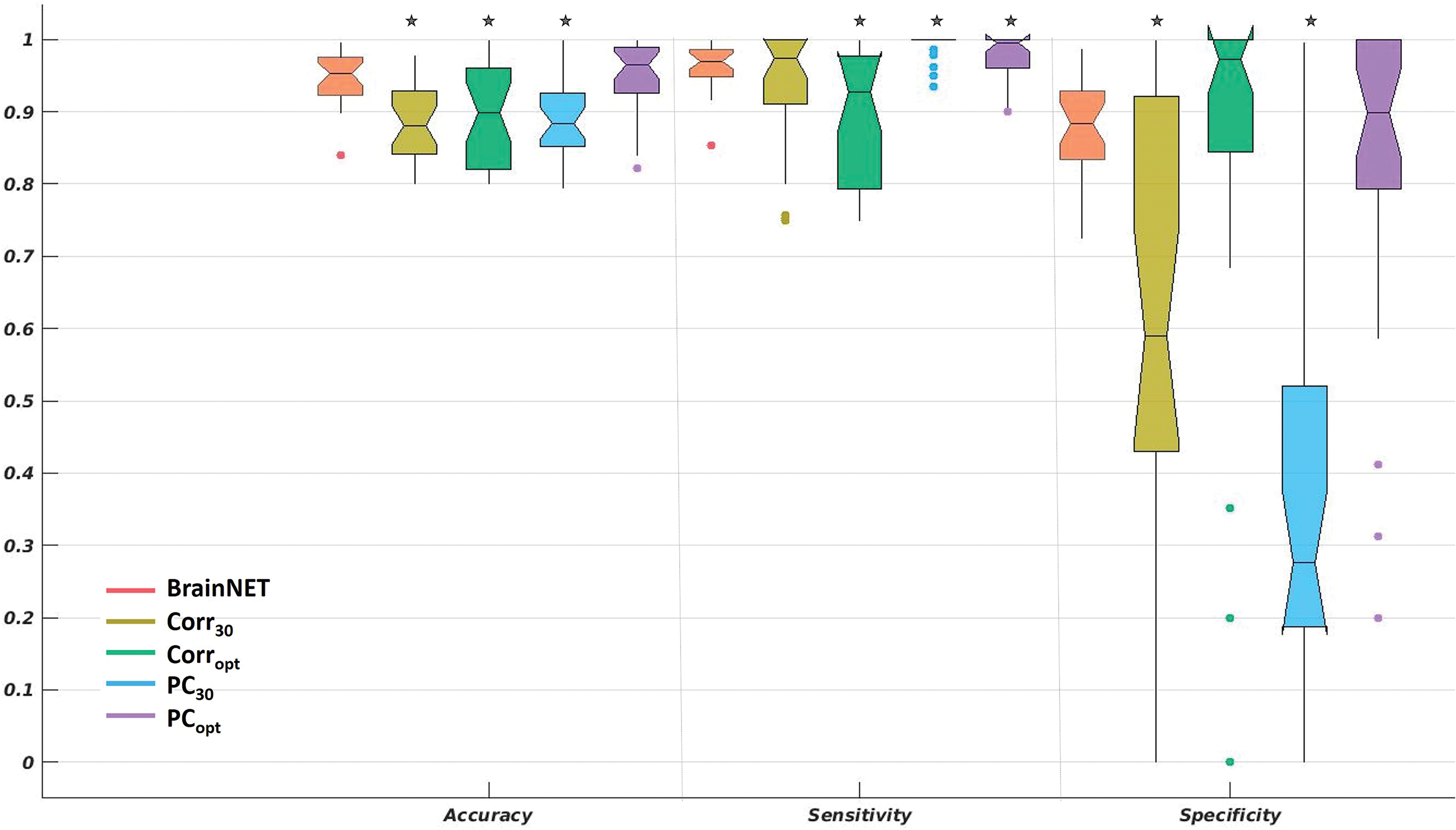
Evaluation of inference methods under varying thresholds. Boxplots of accuracy (left), sensitivity (middle), and specificity (right) across 28 simulations for correlation and PC for optimum and 30% threshold (Corr_opt, Corr₃₀, PC_opt and PC₃₀), and BrainNET. * Represents statistically significant differences from BrainNET performance. Color images are available online.

FIG. 5.

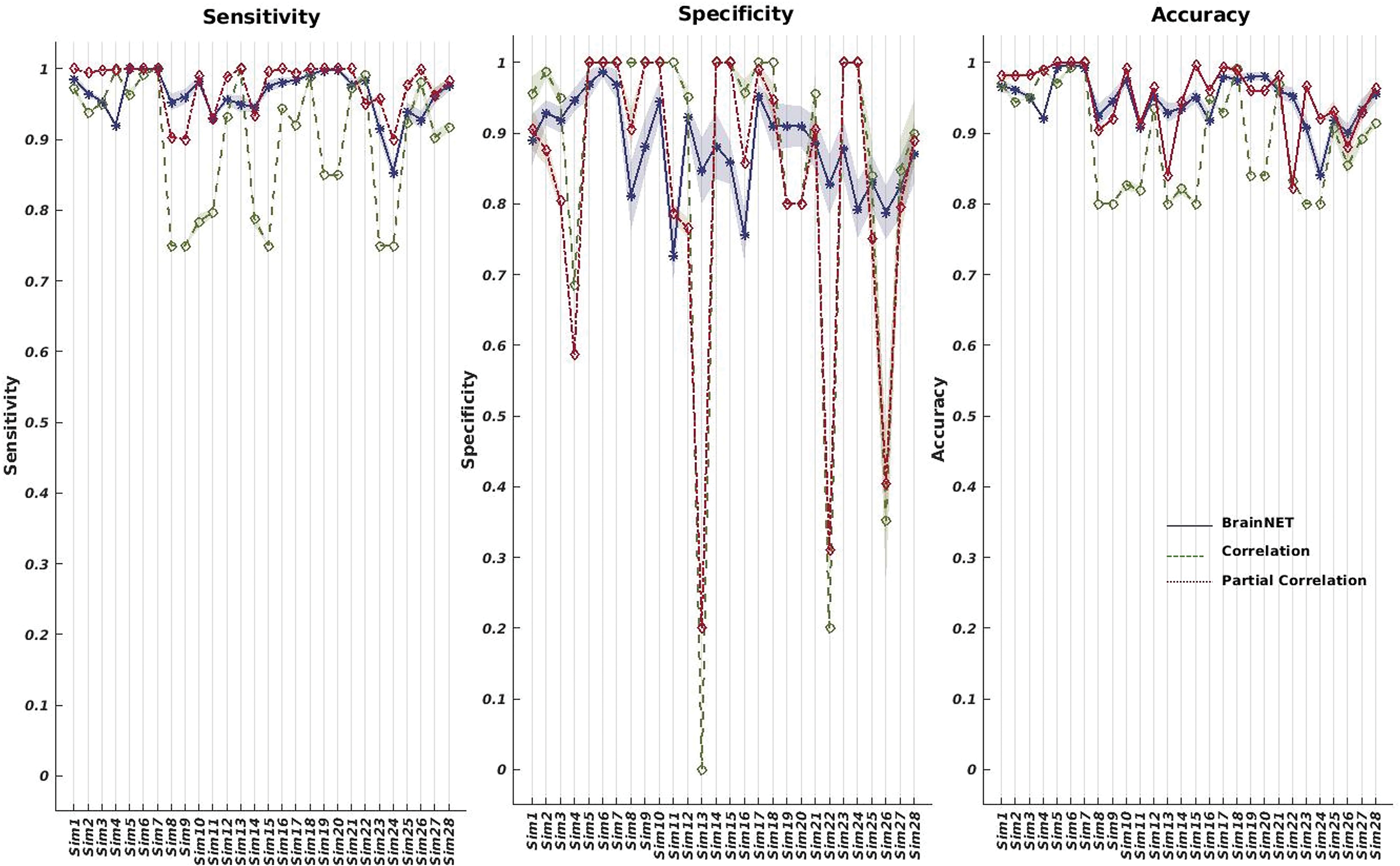
Comparison of correlation (Corr_opt) and PC (PC_opt) at their optimum threshold to BrainNET. Accuracy (left), sensitivity (middle), and specificity (right) for correlation, BrainNET, and PC for 28 simulations. Sensitivity, specificity, and accuracy are all robust across different simulation cases, while PC and correlation methods show fluctuations even with their optimal threshold for functional connectivity. Color images are available online.

The study on effect of simulation parameters on sensitivity and specificity after threshold for BrainNET, PC_opt, and Corr_opt showed that the sensitivity of the inference methods does not get affected by the simulation parameters (Fig. 3B). The specificity of the correlation and PC methods was negatively affected even at their optimum threshold in the presence of backward connections. It is important to note that the specificity and sensitivity were calculated after we thresholded the connectivity matrices from each of these methods (1/number of nodes for BrainNET and optimum threshold for others). After the threshold, BrainNET's performance became robust and consistent across all the simulation parameters.

Evaluation of inference methods on ADHD data

BrainNET was able to identify significant changes (p < 0.05) in global network efficiency, network density, CPL, BC, and shortest path in the ADHD data. Correlation and PC were not able to detect significant changes in any of the whole-brain analyses (Corr₂₀, Corr₃₀, PC₂₀, and PC₃₀).

TDC and ADHD

Statistical analysis of the BrainNET adjacency matrix demonstrated a significant decrease in global network efficiency, an increase in CPL, and an increase in the shortest path length in the right medial temporal gyrus in ADHD compared with TDC (Fig. 7A). While the analysis of the correlation adjacency matrix did not show any significant changes, the PC₃₀ demonstrated a trending increase in CPL in ADHD compared with TDC (p = 0.07). BC and node level local efficiency did not show any changes between the groups in any of the three methods.

TDC and ADHD-I

Statistical analysis of the BrainNET adjacency matrix demonstrated a significant decrease in global network efficiency, a decrease in density, an increase in CPL, and an increase in the shortest path length in the right superior orbital, right Heschl's gyrus, and right medial temporal gyrus nodes in the ADHD-I group compared with TDC (Fig. 7A). The correlation method did not show any relationship between the groups. No relationship was found in other graph metrics studied in any of the methods.

TDC and ADHD-C

Statistical analysis of the BrainNET adjacency matrix demonstrated a significant decrease in density. No significant relationship was found in any other graph metrics for any of the three methods.

ADHD-I and ADHD-C

Statistical analysis of the BrainNET adjacency matrix demonstrated a significant decrease in global network efficiency, a decrease in density, an increase in CPL, and an increase in shortest path length of the right olfactory node (Fig. 7A). A significant increase in BC of the right precuneus node in the ADHD-I group compared with ADHD-C was observed for BrainNET (Fig. 7B). No relationship was found in other graph metrics studied for any of the methods.

Discussion

BrainNET was developed to infer brain network topology using ERT (Geurts et al., 2006). The ERT regressor is used to develop a tree-based ensemble model to predict each node's time series from all other node time series. The tree-based ensemble methods are ideal for inferring complex functional brain networks as they are efficient in learning nonlinear patterns even where there are a large number of features (Wehenkel et al., 2017). The importance matrix is then thresholded to generate an adjacency matrix representing the fMRI topology. The BrainNET model is applicable to both resting-state and task-based fMRI network analysis. It can be easily adapted to data sets with varying session lengths and can be used with different parcellation schemes. A unique feature of the BrainNET approach is that it is implemented at the subject level. It does not need to be trained on big data sets as it infers the network topology based on each individual subject's data.

BrainNET inference of network topology in simulated fMRI data

Evaluation of inference methods using c-sensitivity

BrainNET demonstrated excellent performance across all the simulations and varying confounders. It achieved a significantly higher c-sensitivity than correlation (p < 0.05) and equivalent to PC (p = 0.38) (Fig. 2A). BrainNET performance remained high in the simulations across varying session lengths, number of nodes, neural lags, cyclic connections, and changing number of connections. BrainNET performed weakest in simulations with one primary strong external source around the network. This causes every node to be highly correlated with other nodes and it becomes very difficult to distinguish direct from indirect connections (Smith et al., 2011). It is important to highlight that this kind of one strong external input just for one node is highly unlikely in real-life scenarios. BrainNET, similar to PC and correlation methods, was affected by selection of bad ROIs with time series mixed between them. In this simulation, there are 10 nodes, and each node shares a relatively small amount of the other node time series in a proportion of 0.8:0.2. Since the features have shared data between the nodes in this simulation, it limits discrimination of true connectivity between nodes. The leakage of data between nodes can be minimized in fMRI analysis by selecting independent regions using functionally derived parcellation or methods such as independent component analysis.

One concern with this approach is that as the number of nodes increases, the threshold [1/(number of nodes)] similarly decreases and may result in increased FPs at this low threshold value. The study on effect of number of nodes on the c-sensitivity of BrainNET shows that c-sensitivity of BrainNET does not get affected by the number of nodes (Fig. 2B). This can be interpreted that the ability of BrainNET to distinguish between TP and FPs increases with the increasing number of nodes and the corresponding lower threshold values do not necessarily affect its inference.

Shared inputs between the nodes can be thought of as distinct sensory inputs that feed into one or more nodes. These shared inputs between the nodes could be deleterious if not modeled (Smith et al., 2011). BrainNET is robust to the shared inputs between the nodes, whereas c-sensitivity of PC and correlation is negatively affected (Fig. 2B). The performance on varying connection strengths over time was tested by simulations of stationary/nonstationary connection strengths between the nodes. BrainNET was least affected by nonstationary connection strengths between the nodes (Fig. 2B). The robust performance of BrainNET in simulations with increasing number of nodes, TR, shared inputs, and backward, cyclic, and nonstationary connections represents a promising aspect of the BrainNET method for inferring brain network topology in real-life experimental data (Fig. 2B).

Evaluation of inference methods using thresholds

In this study, we compared the performance of correlation and PC in inferring underlying network topology at optimum threshold values estimated using ground truth (Corr_opt and PC_opt). We also compared the performance of these methods against BrainNET at 30% threshold (Corr₃₀ and PC₃₀) (Fig. 4). BrainNET performed significantly better than PC₃₀, Corr₃₀, and Corr_opt (p < 0.05). At its optimum threshold, PC_opt performed relatively equivalent to BrainNET in terms of accuracy. However, PC_opt showed decreased specificity with increasing number of nodes (sim1–4) and the presence of nonstationary and backward connections (sim13 and sim22) (Fig. 5). Nonstationary connections represent the varying strengths of connections between nodes, which are believed to be similar to those at the neuronal level and being studied in fMRI. The higher sensitivity and lower specificity of PC_opt represent higher numbers of FP connections, which will affect the statistical power of group analysis. The results show that the performance of the PC and correlation method varies under different thresholds and that BrainNET had a better performance than these methods even in their optimum (PC_opt and Corr_opt) (Fig. 4). The study on the effect of the number of nodes on c-sensitivity of BrainNET shows robust performance across all the confounders.

A major strength of the BrainNET approach is that it provides a unique threshold to determine the true network topology. In correlation-based approaches, there is no defined correlation cutoff to determine the true network topology. Instead, multiple approaches are used, or multiple thresholds are applied to generate different networks. Typically, the network cost has been used to define the cutoff value for defining true connections in correlation-based approaches (Supekar et al., 2009). Multiple costs are then applied to generate multiple instances of the network topology, and analyses are performed to determine the variation in network metrics across these costs, or variation in group differences across thresholds (Achard and Bullmore, 2007). The BrainNET approach provides a single threshold obviating the need for these imprecise and convoluted thresholding approaches.

Evaluation of inference methods on ADHD data

Global metrics

Previous studies have shown that ADHD is often associated with changes in the functional organization of the brain and lower network efficiencies in ADHD (Lin et al., 2014; Sidlauskaite et al., 2015). BrainNET was effective in identifying the subtle changes in the ADHD subjects and supports the notion that the functional organization of brain changes in ADHD (Fig. 6) by identifying statistically significant changes in graph metrics between ADHD subjects and TDC.

FIG. 6.

Global graph metrics. The probability density functions and boxplots of global graph metrics with significant changes (p < 0.05) between the groups, ADHD (both ADHD-I and ADHD-C), ADHD-I, ADHD-C, and TDC. ADHD, attention-deficit/hyperactivity disorder; ADHD-C, ADHD combined; ADHD-I, ADHD inattentive; CPL, characteristic path length; TDC, typically developing children. For ease of reading and color images, the figure can be viewed online.

Our results demonstrate that there is a decrease in density and network efficiency, and an increase in CPL in ADHD compared with TDC. A decrease in density suggests that the number of connections is decreased in ADHD compared with TDC. This can be interpreted as an increase in the cost of wiring in the brain. The increase in CPL and the decrease in network efficiency are expected, given that there is a decrease in density suggesting that there is increased difficulty in transferring information across the brain in ADHD. The observed abnormalities in global network topology were identified in ADHD-I, but not in participants with ADHD-C compared with TDC, however, changes between the ADHD-C and ADHD-I were observed. The differential changes observed between the ADHD subtypes may reflect clinical distinctions between the inattentive and combined subtypes of ADHD. Further investigations may shed light on detailed brain-behavior phenotype associations in this neuropsychiatric disorder (Barber et al., 2015; Qian et al., 2019).

Local metrics

BrainNET identified increased NSPL in ADHD-I compared with ADHD-C, suggesting lesser integration of the prefrontal cortex (PFC) in ADHD-I. The PFC is a part of the default mode network (DMN) and plays a crucial role in regulating attention, behavior, and emotion, with the right hemisphere specialized for behavioral inhibition (Arnsten, 2009). The DMN refers to the brain circuitry that includes the medial PFC, posterior cingulate, precuneus, and the medial, lateral, and inferior parietal cortices (Weyandt et al., 2013). These results support previous studies demonstrating that ADHD is associated with structural changes and decreased function of the PFC circuits, especially in the right hemisphere (Arnsten, 2009). BrainNET also demonstrated that BC of the right precuneus, also a part of DMN, was increased in ADHD-I compared with the ADHD-C group. This suggests increased influence of the precuneus in ADHD-I (Fig. 7B). Abnormalities within the DMN have also been found in children in previous studies with ADHD and especially changes in centrality of the right precuneus, which is an important discriminatory feature for classifying ADHD-I and ADHD-C (dos Santos Siqueira et al., 2014).

FIG. 7.

Node level graph metrics. Nodes with significant increases in NSPL in ADHD-I compared with ADHD-C (orange) and in ADHD-I compared with ADHD-C (red) are plotted in the left. Nodes with significant increases in betweenness centrality in ADHD-I compared with ADHD-C are plotted on the right. NSPL, nodal shortest path length. Color images are available online.

Our results also show that the NSPL of the right Heschl's gyrus and right medial temporal gyrus is increased in the ADHD-I group compared with TDC. The NSPL of the olfactory cortex was increased in ADHD-I compared with ADHD-C (Fig. 7A). Deficits in olfactory function are found in neurodegenerative and neuropsychiatric disorders and represent a topic of interest in ADHD (Ghanizadeh et al., 2012). Increased NSPL was found in the right olfactory region in ADHD-I compared with ADHD-C, suggesting lesser integration. Deficits in olfactory ability have been linked to impulsive tendencies within the healthy population and have discriminatory features in identifying people at risk of impulse-control-related problems, supporting the planning of early clinical interventions (Herman et al., 2018). Further studies are required to investigate whether the functional network topology can be used as a biological marker for early diagnosis, treatment, and prognosis of ADHD.

It is important to note that the proposed method measures nonlinear relationships, while the correlation methods measure linear relationships, which may have resulted in the lower performance of correlation in inferring nonlinear brain dynamics. Although PC performed relatively similarly to BrainNET in the simulation data, it did not achieve statistical significance in the ADHD data. This may be due to the FPs identified reducing the statistical power of the analysis. BrainNET can be added to the standard inference methods such as PC and correlation methods, by using a mask derived from the BrainNET importance matrix and applying to the correlation matrix. The output from this combined method will have nodes determined by BrainNET, with Pearson correlation values assigned between the connections. This will avoid using arbitrary thresholds, increase the specificity of the standard inference methods by adding nonlinearity and allowing analysis of connectivity changes between nodes, which cannot be performed with an adjacency matrix derived only from BrainNET.

Limitations

BrainNET takes relatively longer to infer the adjacency matrix than the correlation method. BrainNET took ∼3 sec per subject, whereas the correlation and PC methods just took 0.001 and 9.3 sec, respectively. Longer running time makes BrainNET challenging to apply for voxel-wise analysis.

Conclusion

We describe BrainNET, a new network inference method, to estimate fMRI connectivity that was adapted from gene regulatory methods. We validated the proposed model on ground truth simulation data (Smith et al., 2011). BrainNET outperformed Pearson correlation in terms of accuracy and sensitivity across simulations and various confounders such as the presence of cyclic connections, and even with truncated fMRI sessions of only 2.5 min. We evaluated the performance of BrainNET on the open-source “ADHD 200 preprocessed” data from Neuro Bureau. BrainNET was able to identify significant changes in global graph metrics between ADHD groups and TDC, whereas correlation and PC were unable to find any differences. BrainNET can be used independently or combined with other existing methods as a useful tool to understand network changes and to determine the true network topology of the brain under various conditions and disease states.

Footnotes

Author Contributions

Gowtham Krishnan Murugesan conceptualized and designed the work, analyzed and interpreted the data, and wrote the article. Dr. Joseph Maldjian and Dr. Won Hwa Kim provided expert knowledge and mentorship to develop the method. Ben Wagner contributed in developing fMRI analysis. Chandan Ganesh, Sahil Nalawade, and Dr. Elizabeth Davenport contributed in reviewing the article.

Author Disclosure Statement

No competing financial interests exist.

Funding Information

No funding was received for this article.

Supplementary Material

Supplementary Figure S1

Supplementary Table S1

Supplementary Table S2

Supplementary Table S3

References

Abraham

, Pedregosa

, Eickenberg

, Gervais

, Mueller

, Kossaifi

, et al. 2014. Machine learning for neuroimaging with scikit-learn. Front Neuroinformatics, 8:14.

Achard

, Bullmore

. 2007. Efficiency and cost of economical brain functional networks. PLoS Comput Biol, 3:e17.

Arnsten

FTA.

2009. The emerging neurobiology of attention deficit hyperactivity disorder: the key role of the prefrontal association cortex. J Pediatr, 154:I-S43.

Avena-Koenigsberger

, Misic

, Sporns

. 2018. Communication dynamics in complex brain networks. Nat Rev Neurosci, 19:17.

Barber

, Jacobson

, Wexler

, Beth Nebel

, Caffo

, Pekar

, Mostofsky

. 2015. Connectivity supporting attention in children with attention deficit hyperactivity disorder. Neuroimage Clin, 7:68–81.

Bellec

, Chu

, Chouinard-Decorte

, Benhajali

, Margulies

, Cameron Craddock

. 2017. The neuro bureau ADHD-200 preprocessed repository. Neuroimage, 144:275–286.

Buckner

, Sepulcre

, Talukdar

, Krienen

, Liu

, Hedden

, et al. 2009. Cortical hubs revealed by intrinsic functional connectivity: mapping, assessment of stability, and relation to Alzheimer's disease. J Neurosci, 29:1860–1873.

Camacho

, Collins

, Powers

, Costello

, Collins

. 2018. Next-generation machine learning for biological networks. Cell, 173:1581–1592.

Chen

, Zhang

, Gao

, Wee

C-Y

, Li

, Shen D; Alzheimer's Disease Neuroimaging

Initiative

. 2016. High-order resting-state functional connectivity network for MCI classification. Hum Brain Mapp, 37:3282–3296.

10.

Cortese

, Kelly

, Chabernaud

, Proal

, Di Martino

, Milham

, Castellanos

. 2012. Toward systems neuroscience of ADHD: a meta-analysis of 55 fMRI studies. Am J Psychiatry, 169:1038–1055.

11.

Crossley

, Mechelli

, Scott

, Carletti

, Fox

, McGuire

, Bullmore

. 2014. The hubs of the human connectome are generally implicated in the anatomy of brain disorders. Brain, 137:2382–2395.

12.

dos Santos Siqueira

, Anderson, Biazoli Junior

, Comfort

, Rohde

, ato

. 2014. Abnormal functional resting-state networks in ADHD: graph theory and pattern recognition analysis of fMRI data. Biomed Res Int, 2014:380531.

13.

Finkle

, Wu

, Bagheri

. 2018. Windowed Granger causal inference strategy improves discovery of gene regulatory networks. Proc Natl Acad Sci U S A, 115:2252–2257.

14.

Fornito

, Zalesky

, Breakspear

. 2015. The connectomics of brain disorders. Nat Rev Neurosci, 16:159–172.

15.

Fornito

, Zalesky

, Bullmore

. 2016. Fundamentals of Brain Network Analysis. Cambridge, MA: Academic Press; p. 301.

16.

Fortin

J-P

, Cullen

, Sheline

, Taylor

, Aselcioglu

, Cook

, et al. 2018. Harmonization of cortical thickness measurements across scanners and sites. Neuroimage, 167:104–120.

17.

Geurts

, Ernst

, Wehenkel

. 2006. Extremely randomized trees. Mach Learn, 63:3–42.

18.

Ghanizadeh

, Bahrani

, Miri

, Sahraian

. 2012. Smell identification function in children with attention deficit hyperactivity disorder. Psychiatry Investig, 9:150.

19.

Hagberg

, Schult

, Swart

, Conway

, Séguin-Charbonneau

, Ellison

, et al. 2013. Networkx. High productivity software for complex networks. https://networkx.lanl.gov/wiki Last accessed March 21, 2020 .

20.

Herman

, Critchley

, Duka

. 2018. Decreased olfactory discrimination is associated with impulsivity in healthy volunteers. Sci Rep, 8:15584.

21.

Hilger

, Fiebach

. 2019. ADHD symptoms are associated with the modular structure of intrinsic brain networks in a representative sample of healthy adults. Netw Neurosci, 3:567–588.

22.

Irrthum

, Wehenkel

, Geurts

. 2010. Inferring regulatory networks from expression data using tree-based methods. PLoS One, 5:e12776.

23.

Kim

, Adluru

, Chung

, Okonkwo

, Johnson

, Bendlin

, Singh

. 2015. Multi-resolution statistical analysis of brain connectivity graphs in preclinical Alzheimer's disease. Neuroimage, 118:103–117.

24.

Kim

, Racine

, Adluru

, Jae Hwang

, Blennow

, Zetterberg

, et al. 2019. Cerebrospinal fluid biomarkers of neurofibrillary tangles and synaptic dysfunction are associated with longitudinal decline in white matter connectivity: a multi-resolution graph analysis. Neuroimage Clin, 21:101586.

25.

Lin

, Sun

, Yu

, Wu

, Yang

, Liang

, Liu

. 2014. Global and local brain network reorganization in attention-deficit/hyperactivity disorder. Brain Imaging Behav, 8:558–569.

26.

Milham

, Fair

, Mennes

, Mostofsky

SHMD

. 2012. The ADHD-200 consortium: a model to advance the translational potential of neuroimaging in clinical neuroscience. Front Syst Neurosci, 6:62.

27.

Murugesan

, Saghafi

, Davenport

, Wagner

, Urban

, Kelley

, et al. 2018. Single season changes in resting state network power and the connectivity between regions: distinguish head impact exposure level in high school and youth football players. Proc SPIE Int Soc Opt Eng, 10575:105750F1–105750F7.

28.

O'Neill

, Davenport

, Murugesan

, Montillo

, Maldjian

. 2017. Applications of resting state functional mr imaging to traumatic brain injury. Neuroimaging Clin, 27:685–696.

29.

Pellegrini

, Ballerini

, Hernandez

MdCV

, Chappell

, González-Castro

, Anblagan

, et al. 2018. Machine learning of neuroimaging to diagnose cognitive impairment and dementia: a systematic review and comparative analysis. arXiv Preprint arXiv:1804.01961.

30.

Petralia

, Wang

, Yang

, Tu

. 2015. Integrative random forest for gene regulatory network inference. Bioinformatics, 31:i197–i205.

31.

Praagman

1985. Classification and regression trees. In: Breiman

, Friedman

, Olshen

, Stone

(eds.) The Wadsworth Statistics/Probability Series. Belmont, CA: Wadsworth; p. 144.

32.

Qian

, Castellanos

, Uddin

, Yi Loo

, Liu

, Li Koh

, et al. 2019. Large-scale brain functional network topology disruptions underlie symptom heterogeneity in children with attention-deficit/hyperactivity disorder. Neuroimage Clin, 21:101600.

33.

Saeed

2018. Towards quantifying psychiatric diagnosis using machine learning algorithms and big fMRI data. Big Data Analytics, 3:7.

34.

Sidlauskaite

, Caeyenberghs

, Sonuga-Barke

, Roeyers

, Wiersema

. 2015. Whole-brain structural topology in adult attention-deficit/hyperactivity disorder: preserved global–disturbed local network organization. Neuroimage Clin, 9:506–512.

35.

Smith

, Miller

, Salimi-Khorshidi

, Webster

, Beckmann

, Nichols

, et al. 2011. Network modelling methods for FMRI. Neuroimage, 54:875–891.

36.

Sporns

2018. Graph theory methods: applications in brain networks. Dialogues Clin Neurosci, 20:111.

37.

Stam

, Reijneveld

. 2007. Graph theoretical analysis of complex networks in the brain. Nonlinear Biomed Phys, 1:3.

38.

Strobl

, Boulesteix

A-L

, Zeileis

, Hothorn

. 2007. Bias in random forest variable importance measures: illustrations, sources and a solution. BMC Bioinformatics, 8:25.

39.

Supekar

, Musen

, Menon

. 2009. Development of large-scale functional brain networks in children. PLoS Biol, 7:e1000157.

40.

Turki

, Wang

JTL

, Rajikhan

. Inferring gene regulatory networks by combining supervised and unsupervised methods. In 2016 15th IEEE International Conference on Machine Learning and Applications (ICMLA). Anaheim, CA: IEEE, 2016, pp. 140–145.

41.

Tzourio-Mazoyer

, Landeau

, Papathanassiou

, Crivello

, Etard

, Delcroix

, et al. 2002. Automated anatomical labeling of activations in SPM using a macroscopic anatomical parcellation of the MNI MRI single-subject brain. Neuroimage, 15:273–289.

42.

Waller

, Brovkin

, Dorfschmidt

, Bzdok

, Walter

, Kruschwitz

. 2018. GraphVar 2.0: a user-friendly toolbox for machine learning on functional connectivity measures. J Neurosci Methods, 308:21–33.

43.

Wang

, Wang

, Xia

, Liao

, Evans

, He

. 2015. GRETNA: a graph theoretical network analysis toolbox for imaging connectomics. Front Hum Neurosci, 9:386.

44.

Wang

, Zuo

, He

. 2010. Graph-based network analysis of resting-state functional MRI. Front Syst Neurosci, 4:16.

45.

Warren

, Power

, Bruss

, Denburg

, Waldron

, Sun

, et al. 2014. Network measures predict neuropsychological outcome after brain injury. Proc Natl Acad Sci U S A, 111:14247–14252.

46.

Wehenkel

, Bastin

, Phillips

, Geurts

. Tree ensemble methods and parcelling to identify brain areas related to Alzheimer's disease. In 2017 International Workshop on Pattern Recognition in Neuroimaging (PRNI). Toronto, Canada: IEEE, 2017, pp. 1–4.

47.

Weyandt

, Swentosky

, Gudmundsdottir

. 2013. Neuroimaging and ADHD: fMRI, PET, DTI findings, and methodological limitations. Dev Neuropsychol, 38:211–225.

48.

Williams

, Henson

. 2018. Recent Advances in Functional Neuroimaging Analysis for Cognitive Neuroscience. London, England: SAGE Publications.

49.

Yamashita

, Yahata

, Itahashi

, Lisi

, Yamada

, Ichikawa

, et al. 2019. Harmonization of resting-state functional MRI data across multiple imaging sites via the separation of site differences into sampling bias and measurement bias. PLoS Biol, 17:e3000042.

50.

Yan

, Zhang

, Sui

, Shen

. 2018. Deep chronnectome learning via full bidirectional long short-term memory networks for MCI diagnosis. In International Conference on Medical Image Computing and Computer-Assisted Intervention. Granada, Spain: Springer, 2018, pp. 249–257.

51.

, Zhang

, An

, Chen

, Wei

, Shen

. 2017. Connectivity strength-weighted sparse group representation-based brain network construction for MCI classification Hum Brain Mapp, 38:2370–2383.

52.

Zaharchuk

, Gong

, Wintermark

, Rubin

, Langlotz

. 2018. Deep learning in neuroradiology. Am J Neuroradiol, 39:1776–1784.

53.

Zhou

, Chen

, Zhang

, Hu

, Qiao

, Yu

, et al. 2020. A toolbox for brain network construction and classification (BrainNetClass). Hum Brain Mapp, 41:2808–2826.

Supplementary Material

Please find the following supplemental material available below.

For Open Access articles published under a Creative Commons License, all supplemental material carries the same license as the article it is associated with.

For non-Open Access articles published, all supplemental material carries a non-exclusive license, and permission requests for re-use of supplemental material or any part of supplemental material shall be sent directly to the copyright owner as specified in the copyright notice associated with the article.

0.00 MB

0.02 MB

0.01 MB

0.02 MB

5.84 MB