Real-Time Resting-State Functional Magnetic Resonance Imaging Using Averaged Sliding Windows with Partial Correlations and Regression of Confounding Signals

Abstract

Background/Introduction:

There is considerable interest in using real-time functional magnetic resonance imaging (fMRI) for monitoring functional connectivity dynamics. To date, the majority of real-time resting-state fMRI studies have examined a limited number of brain regions. This is, in part, due to the computational demands of traditional seed- and independent component analysis-based methods, in particular when using increasingly available high-speed fMRI methods.

Methods:

This study describes a computationally efficient, real-time, seed-based, resting-state fMRI analysis pipeline using moving averaged sliding-windows (ASW) with partial correlations and regression of motion parameters and signals from white matter and cerebrospinal fluid.

Results:

Analytical and numerical analyses of ASW correlation and sliding-window regression as a function of window width show selectable bandpass filter characteristics and effective suppression of artifactual correlations resulting from signal drifts and transients. The analysis pipeline is compatible with multislab echo-volumar imaging and simultaneous multislice echo-planar imaging with repetition times as short as 136 msec. High-speed, resting-state fMRI data in healthy controls demonstrate the effectiveness of this approach for minimizing artifactual correlations in white and gray matter, which was comparable to conventional regression across the entire scan. Integrating sliding-window averaging (width: W ₁) within a second-level sliding-window (width: W ₂) enabled monitoring of intra- and internetwork correlation dynamics of up to 12 resting-state networks with bandpass filter characteristics determined by the first-level sliding-window and temporal resolution W ₁ + W ₂.

Conclusions:

The computational performance and confound tolerance make this seed-based, resting-state fMRI approach suitable for real-time monitoring of data quality and resting-state connectivity dynamics in neuroscience and clinical research studies.

Impact statement

Using averaged sliding-windows for seed-based correlation and regression of confounding signals provides a powerful model-free approach to increase tolerance to artifactual signal transients in resting-state analysis. The algorithmic efficiency of this sliding-window approach enables real-time, seed-based, resting-state functional magnetic resonance imaging (fMRI) of multiple networks with computation of connectivity matrices and online monitoring of data quality. Integration of a second-level sliding-window enables mapping of resting-state connectivity dynamics. Sensitivity and tolerance to confounding signals compare favorably with conventional correlation and confound regression across the entire scan. This methodological advance has the potential to enhance the clinical utility of resting-state fMRI and facilitate neuroscience applications.

Introduction

Resting-state connectivity is currently studied in a wide range of neuroscience and clinical applications with more than 100 resting-state networks identified in group studies and interindividual differences in network topology detectable in individual subjects (Allen et al., 2011; D'Esposito, 2019; Gordon et al., 2017; Smith et al., 2013). Real-time, resting-state functional magnetic resonance imaging (fMRI) is an emerging technology (Esposito et al., 2003; Kim et al., 2015; Megumi et al., 2015; Monti et al., 2017; Posse et al., 2013; Vakamudi et al., 2020; Zilverstand et al., 2014) that has been explored in a few feasibility studies (Koush et al., 2013, 2017), in addition to task-based, real-time fMRI (Misaki et al., 2018; Young et al., 2018), to investigate changes in functional connectivity with neurofeedback.

Monitoring of resting-state network dynamics in real time may enhance data quality control, support decision-making to adapt a scanning strategy, and stabilize a subject's level of attention and wakefulness to maximize sensitivity and specificity. In the clinical setting, this approach has the potential to increase scan success, and reduce scan time and overall cost. However, analysis tools that are suitable for real-time, resting-state fMRI, such as cortex-based independent component analysis (ICA) (Esposito et al., 2003; Soldati et al., 2013a, 2013b), region of interest (ROI)-based connectivity between network nodes (Kim et al., 2015; Megumi et al., 2015; Monti et al., 2017; Zilverstand et al., 2014), and seed-based, whole-brain connectivity (Posse et al., 2013; Vakamudi et al., 2020), are currently only at the feasibility stage (Margulies et al., 2010).

Real-time, resting-state fMRI, in particular when using sliding-windows to monitor temporal dynamics, is highly sensitive to a wide range of confounds, including movement, which obscure networks as well as create false-positive correlations (Satterthwaite et al., 2012, 2013; Van Dijk et al., 2012), physiological noise (cardiovascular and respiratory pulsations) (Liu, 2016; Triantafyllou et al., 2011), and scanner instabilities. A real-time, motion analytics tool that allows censoring of data frames affected by head movement and provides statistics to determine the scan time necessary to collect a desired amount of low movement data has recently been described (Dosenbach et al., 2017). Regression of confounds is widely used in resting-state fMRI (Behzadi et al., 2007; Glover et al., 2000; Muschelli et al., 2014), and the feasibility of real-time, resting-state fMRI with regression of physiological noise using a general linear model-based approach implemented in a graphic processing unit has recently been described (Misaki et al., 2015).

Increasingly available high-speed fMRI methods, such as simultaneous multislice echo-planar imaging (SMS-EPI) (Feinberg et al., 2010; Setsompop et al., 2012), magnetic resonance encephalography (Zahneisen et al., 2011), and multislab echo-volumar imaging (MS-EVI) (Posse et al., 2012), enable unaliased measurement of physiological noise to increase sensitivity in resting-state fMRI. However, few real-time fMRI analysis tools offer the processing performance required for high-speed fMRI.

In the current study, we describe a computationally efficient, real-time, seed-based, resting-state fMRI analysis pipeline using moving averaged sliding-windows (ASW) with partial correlations and regression of motion parameters and signals from white matter (WM) and cerebrospinal fluid (CSF), which in our preliminary studies demonstrated tolerance to head movement, signal drifts, and physiological signal pulsation (Posse et al., 2013; Vakamudi et al., 2020). We perform analytical and numerical analyses of this approach, evaluate the computational performance for high-speed fMRI with repetition times (TR) as short as 136 msec, and assess in vivo the suppression of artifactual correlations in white and gray matter in comparison with full window regression (FWR). We then introduce a second-level sliding-window approach to monitor intra- and internetwork correlation dynamics.

Methods and Materials

Analytical analysis of ASW correlation

Averaging of sliding-windows provides high-pass filter characteristics determined by the window width, similar to non-ASW (Leonardi and Van De Ville, 2015), which reduce the effects of low-frequency drifts. The combination of ASW with a moving average low-pass filter provides an effective bandpass filter that depends on the widths of the sliding-window and the moving average filter (MAF) to attenuate both low frequencies and physiological signal pulsation. The frequency responses of the ASW and the MAF with Hamming window were calculated numerically and analytically, respectively, and convolved together. The passband response is shown in Figure 1. While the transition bands with this approach are not as steep as the traditional finite impulse response or infinite impulse response bandpass filters, it is effective for reducing physiological noise (Lin et al., 2012) and can be applied in real time with minimal computational cost and time lag. The addition of a Hamming window reduces the amplitudes of sidebands in the frequency domain and provides ∼40 dB attenuation in the high-frequency range.

FIG. 1.

Bandpass frequency response of high-pass moving average SW correlation combined with Hamming-filtered low-pass MAF. (a) Frequency response for SW width: 15 sec and MAF width: 2 sec using a 100% Hamming window. (b) Low-frequency cutoff at −30 dB as a function of SW width and MAF width. (c) High-frequency cutoff at −30 dB as a function of MAF width and SW width for different Hamming filters. MAF, moving average filter; SW, sliding-window. Color images are available online.

Averaging of sliding-window correlation maps additionally reduces the confounding effect of signal transients as these are confined to a limited number of windows and are averaged out (Posse et al., 2013). To characterize confound suppression, we considered the correlation coefficient between two signals x and y, which is defined as follows:

$r = \frac{N \sum x y - \sum x \sum y}{{\{(N \sum x^{2} - {(\sum x)}^{2}) (N \sum y^{2} - {(\sum y)}^{2})\}}^{1 ∕ 2}}$ (1)

Analytical equations to characterize the over/underestimation of the correlation due to different signal confounds (drifts, offsets, spikes, boxcars) were developed based on Equation 1. The following equations show correlations for the cases of spikes in a single time course (Eq. 3) and simultaneously in both time courses (Eq. 4) using the function f defined in Equation 2. Each spike is modeled as an increase in amplitude at a single time point.

$f (x, y) = N \sum x^{2} - {(\sum x)}^{2} + n_{s} (N - 1) {A_{s}}^{2} + 2 n_{s} A_{s} (N x_{s} - \sum x)$ (2)

$ρ_{1 s p i k e} = \frac{N \sum x y - \sum x \sum y + n_{s} A_{s} (N y_{s} - \sum y)}{{\{f (x, y) (N \sum y^{2} - {(y)}^{2})\}}^{1 ∕ 2}}$ (3)

$\begin{matrix} ρ_{2 s p i k e} = \\ \frac{N \sum x y - \sum x \sum y + n (N - 2) {A_{s}}^{2} + n_{s} A_{s} (N x_{s} + N y_{s} - \sum x - \sum y)}{{\{f (x, y) f (y, x)\}}^{1 ∕ 2}} \end{matrix}$ (4)

where x and y are the spike-free time courses being correlated, N is the number of time points, A_s is the spike amplitude, x_s = mean(x) + A_s , y_s = mean(y) + A_s , and n_s is the number of spikes. Equation 5 shows how sliding-window correlations modify the confounded correlations in Equations 3 and 4:

$ρ_{S W} = \frac{1}{N - ω + 1} \sum_{1}^{N - 2 ω + 1} μ + \frac{n_{s}}{N - ω + 1} \sum_{1}^{ω} ρ_{s p i k e}$ (5)

where μ is the correlation without confounds and ω is the window width. The first term is the contribution from windows that do not sample the spikes, while the second term accounts for the contribution from windows that do sample the spikes. For spike amplitude approaching zero, there is little difference between correlations with various window widths, including conventional, cumulative seed-based approaches (ω = N). As spike strength increases, sliding-window correlations display reduced changes in measured correlations. To further characterize the behavior of this methodology, we take the limit of Equation 5 for large spikes in both time courses, and small values of ω/N:

${lim}_{\frac{ω}{N} \to 0; A_{s} \to \infty} ρ_{S W} = μ + \frac{n_{s} ω}{N}$ (6)

In these limits, the over/underestimation of the correlation due to the spikes decreases linearly with window width and spike number (Eq. 6). This behavior holds for the case of spikes with varying amplitudes and is further explored numerically in the next section.

Numerical simulations of ASW correlation

Two random signals (variance = 1, mean = 0) were generated, filtered using a low-pass filter (∼0.23 Hz), and mixed to induce a known correlation. Rician noise and confounds were added to assess the viability of different window widths (including seed-based analysis with no sliding-window) for reproducing the original correlation. To verify the theoretical behavior predicted in the previous sections, signal spikes were added to one of the time courses and then both of the time courses. Spike number (n) varied from a single instance to randomly distributed spikes of varying numbers (from 2 to 100), either at fixed or various randomly chosen points in the time course. Spike amplitude was also varied from 1 to 10σ (σ—standard deviation [SD]). Other parameter choices made in these simulations approximate standard analysis and did not affect qualitative results.

In addition, simulated signal-to-noise ratios (SNRs) were varied to assess the effectiveness of this approach as a denoising tool with SNR values ranging from 0.1 to 10. Various confound types were modeled and added to one or both time courses to analyze the response of this methodology. These confounds included the following: boxcars, linear drifts, step functions (offsets), spikes, and combinations of these signal profiles. Signal offsets were modeled as a 4σ positive discontinuity in signal intensity halfway through the time course (dx/dt|_t ₌ _T/2 = ∞). Signal drifts were modeled as a simple linear function (dx/dt = 1% of root mean square signal) added to the time course. Boxcar functions were modeled as 4σ positive discontinuity followed by a 4σ negative discontinuity. The width of the boxcar was N/10 and was aligned with the center of the time course.

Numerical analysis of ASW regression

For FWR, the entire signal was regressed before sliding-window correlation analysis, and the sliding-window averaged correlations were then computed between the regressed signals. The sliding-window regression method was implemented based on the detrending approach described in Equation 4 in Gembris et al. (2000). Sliding-window correlation between two signals x and r with regression of L confounding signals s_i was computed as follows:

$ρ = \frac{{\vec{x}}_{S} \vec{r_{S}}}{|{\vec{x}}_{S}| |\vec{r_{S}}|} = \frac{(\vec{x} - \sum_{i = 0}^{L - 1} α_{i} {\vec{s}}_{i}) (\vec{r} - \sum_{i = 0}^{L - 1} β_{i} {\vec{s}}_{i})}{|\vec{x} - \sum_{i = 0}^{L - 1} α_{i} {\vec{s}}_{i}| |\vec{r} - \sum_{\dot{i} = 0}^{L - 1} β_{i} {\vec{s}}_{i}|}$ (7)

where $α_{i}$ and $β_{i}$ are the regression coefficients. Two signal time courses that consisted of single or combinations of sinusoids with varying phases and periodicity, and 2000 time points were generated. A Rician noise distribution with noncentrality and scale parameters of unity was added along with the following signal confounds: boxcars, linear drifts, step functions (offsets), and spikes. These signals were then mixed according to Equation 8 with a mixing coefficient (β) of 0.2, to induce the Pearson correlation (r) of the order of 0.2–0.3.

$s_{1} = (1 - β) s_{1} + β s_{2}$ (8)

where s₁ and s₂ are nonregressed signals 1 and 2, respectively. Sliding-window averaged correlations were calculated before the introduction of signal confounds (no confound case) and after adding signal confounds either to one or to both time courses. The regression process included regression of a constant vector to remove offset effects. Multiple iterations of the simulation using different manifestations of random signals were performed.

All analytical analyses and simulations were performed using custom matrix laboratory (MATLAB, a programming software developed by MathWorks; The MathWorks, Inc., Natick, MA) scripts.

Subjects

Resting-state scans were acquired in 11 right-handed healthy controls (6 females and 5 males) aged between 21 and 55 years. In this Institutional Review Board-approved study, subjects were instructed to clear their mind and try not to think anything in particular, relax, and fixate on a cross-hair presented on a computer screen during eyes-open resting scans.

Data acquisition

Data were collected at the Mind Research Network on a 3T Siemens TIM Trio scanner (Siemens Healthineers, Malvern, PA) equipped with the MAGNETOM Avanto gradient system and a 32-channel head array coil. High-resolution, T₂-weighted Turbo Spin Echo scans were acquired for anatomical reference. FMRI data were acquired in anterior commissure/posterior commissure (AC/PC) orientation using the following:

MS-EVI (Posse et al., 2012) was acquired in five healthy controls using the following: TR/TE (echo time)—136/28 msec, flip angle—10°, number of scans—2276, 2 slabs, spatial matrix—64 × 64 × 8 × 2, voxel size—4 × 4 × 6 mm³, interslab gap—10%, generalized autocalibrating partial parallel acquisition acceleration—4, k_y partial Fourier encoding—6/8, and oversampling along the slab-direction (7/8) resulting in 13 reconstructed slices, scan time: 5:16 min. The in-plane image reconstruction with parallel imaging reconstruction was performed on the scanner. The through-plane reconstruction of MS-EVI was performed online (Posse et al., 2012) on an external Linux workstation using our custom TurboFIRE (Turbo Functional Imaging in Real-time) fMRI analysis tool (Gembris et al., 2000; Posse et al., 2013).

SMS-EPI was acquired in six healthy controls using the following: TR/TE—400/35 msec, flip angle—42°, number of scans: 900, number of slices: 32, spatial matrix—64 × 64 × 32, voxel size—3 × 3 × 3 mm³, interslice gap—0 mm, SMS factor—8, and scan time: 6:08 min. Raw data were preprocessed using the scanner reconstruction computer and sent via a local network connection to an external server (second Linux workstation) for multiband reconstruction calculations. Unaliased data were sent back to the scanner reconstruction computer for parallel imaging reconstruction and postprocessing.

Real-time image transfer (partial header file and reconstructed pixel [picture element] data) to the scanner host computer was performed using an in-house-developed software module (Image Calculation Environment functor) that was integrated into the image reconstruction pipeline, and a server that forwarded images to the TurboFIRE Linux workstation using the transmission control protocol/Internet protocol (TCP/IP). For performance reasons, the transfer of reconstructed images to the image database was disabled.

Data analysis

The reconstructed data were processed using TurboFIRE (version v5.15.28.0) on an Intel Xeon E5-2697 v4 @ 2.30 GHz × 51, 2 × 18 core workstation with 64 GB random access memory (RAM) and 64 Bit Ubuntu operating system 16.04. The C++ software architecture consisted of 11 single-threaded sequential processes for pre- and postprocessing and up to 12 parallel correlator processes with dynamic multithreading (up to 64 threads per correlator) to take advantage of the multiprocessor architecture of the workstation.

Preprocessing (real time and offline)

The preprocessing steps included the following: T₂*-weighted echo averaging (in case of multiecho data) (Posse et al., 1999; Vakamudi et al., 2020), six-parameter rigid body motion correction, isotropic 5 mm spatial smoothing using a Gaussian kernel, spatial normalization using manual selection of the midpoint of the AC/PC line, and mapping of the Montreal Neurological Institute (MNI) atlas into subject space using a lookup table approach (Gao and Posse, 2003), and an 8-sec moving average time domain low-pass filter with a 100% Hamming window width (Lin et al., 2012) to reduce signal fluctuations due to cardiac and respiratory pulsations. The lookup table related coordinates in object space to MNI space using voxel to voxel mapping. Since several voxels in normalized space may be projected to the same voxel in object space, corresponding source locations in normalized space were spatially averaged. The initial 10 sec of data were discarded to account for nonsteady-state signal changes. A maximum of 12 ROIs were simultaneously processed in TurboFIRE to generate time courses for correlation analysis (Gao and Posse, 2004).

Seed selection and tissue masks

Brodmann areas (BAs) were selected as seed regions after transforming the coordinates from the MNI atlas into the Talairach atlas using Matthew Brett's formula and automatically assigned using a modified Talairach Daemon database (Lancaster et al., 2000). For real-time analysis, a 10-sec prescan was spatially normalized to select atlas-based seed regions. WM and CSF seeds for regression were manually delineated. For offline analyses, the following atlas-based networks were mapped in subject-space: sensorimotor network (SMN)—BA1-3, default mode network (DMN)—BA7 and 31, visual network (VSN)—BA17, and auditory network (AUN)—BA41 and 42. For MS-EVI data, WM and CSF seeds for regression were manually delineated. For SMS-EPI data, segmentation-based CSF and WM tissue masks for offline analysis were generated using statistical parametric mapping (SPM) 12 and analysis of functional neuroimages (AFNI; https://afni.nimh.nih.gov/afni). The binary masks were iteratively eroded to minimize partial volume effects.

Resting-state seed-based connectivity analysis

The time courses of up to 12 selected ROIs were designated as seed regions to extract time courses for correlation analysis or as reference regions to extract time courses for regression. Voxel-based, sliding-window (window width: W ₁) partial correlations between the regressed signal time courses $\vec{x_{s}}$ in each pixel and the regressed reference vector $\vec{r_{s}}$ were computed using Equation 7 by adapting the methodology described in Gembris et al. (2000). Sliding-window correlation without regression was based on a fast implementation of Equation 1 (Gembris et al., 2000). The means of the signal and the reference vector were subtracted before correlation. Regressor time courses included the six rigid body motion parameters and manually defined WM and CSF ROIs (in case of real-time analysis) or the spatially averaged time courses from the imported masks of WM and CSF (in case of offline analysis). The regression coefficients were computed for each sliding-window by solving Equations 6 and 7 in Gembris et al. (2000) using the conjugate gradient method. The moving averaging of the resulting sliding-window correlation maps used an efficient running variance algorithm (Welford, 1962) to compute the mean and the SD of correlation maps and combinations thereof (e.g., mean/SD) during the scan (Posse et al., 2013). For comparison, conventional regression across the entire scan was performed using custom MATLAB toolboxes, which used a principal component analysis (PCA)-based approach (Behzadi et al., 2007) that extracts five principal components each from the multivoxel time courses of the WM and CSF masks and averages them.

Nonthresholded (r = 0) and thresholded correlation maps (r = 0.3–0.7) were obtained. A correlation threshold of 0.5 corresponds to a threshold of p < 0.0001 (corrected for family-wise error rates using a third-order autoregressive [AR(3)] model). K-means cluster analyses were performed to record the spatial cluster extent (number of voxels), the maximum (peak), mean, SD of the correlation within each cluster, and the anatomical location of the peak voxel in MNI coordinates within each cluster at a correlation threshold of 0.5. A corresponding cluster analysis across the entire brain was performed for correlation maps obtained with WM seeds using a correlation threshold of 0.5. Correlation coefficients were Fisher Z-transformed. To characterize the effect of sliding-window width, Z-scores and spatial extents (measured in a number of voxels) were normalized within subject to ASW with 30-sec window. To compare the three analysis methods (ASW, averaged sliding-window regression [ASWR], and FWR), Z-scores and spatial extents were normalized within subject to FWR. SDs were computed across subjects.

Computational performance

The computation times for individual processing steps were measured using a profiling feature implemented in TurboFIRE. The latency between image transfer and generation of a fully regressed update of the resting-state correlation map was measured as a function of the number of mapped networks and TR.

Mapping of temporal dynamics of networks and inter-region connectivity

A second-level sliding-window (width: W ₂) that constrained the moving averaging process to the W ₂ most recent (first level) sliding-window correlation maps (window width: W ₁) was implemented to dynamically map the mean and SD and combinations thereof (e.g., mean/SD) for each position of the second-level sliding-window. The effective temporal resolution of this approach was W ₁ + W ₂. To assess the utility of this approach, SMS-EPI data from one subject were processed using W ₁ = 8 sec, W ₂ = 30 sec, 10 sec of discarded images, and an 8-sec MAF with 100% Hamming window. Cluster analyses were performed at selected time intervals after the first acquisition (t ₀) starting at t ₀ + 40 sec to ensure steady-state processing with consistent degrees of freedom. Second-level sliding-window correlations between seed regions were computed from the sliding-window seed signal time courses and displayed in the form of dynamically updated 12 × 12 correlation matrices. To compare this display of internetwork correlations with a recent ICA-based study of resting-state connectivity (Allen et al., 2011), a larger 28 × 28 correlation matrix was computed offline by individually masking 28 seed regions using the peaks of ICA components described in that study that represent major network nodes. The following network nodes and corresponding ICA components from that study (Allen et al., 2011) were selected: attention—independent component (IC) 34, IC52, IC55, IC60, IC71, IC72; auditory—IC17; basal ganglia—IC21; default mode—IC25, IC50, IC53, IC68; frontal—IC20, IC42, IC47, IC49; sensorimotor—IC07, IC23, IC24, IC29, IC38, IC56; and visual—IC39, IC46, IC48, IC59, IC64, IC67. Voxel-based correlation values within these masks were spatially averaged using TurboFIRE and custom MATLAB scripts.

Results

Analytical and numerical analysis of ASW correlation

The suppression of the effects of signal transients using averaging of sliding-window correlations for the case of spikes is shown in Figure 2, which displays the analytical behavior of Equation 5 in a graphical representation with varying window widths (w) and spike strengths (s) and a numerical simulation. The initial correlation between the two signals without spikes in Figure 2a and b is 0.5. When adding a simultaneous spike in both time courses, the correlation reaches unity (Fig. 2a). With decreasing window width, it decreases to the original value of 0.5. When adding a spike in a single time courses, the correlation approaches zero (Fig. 2b). With decreasing window width, it increases back to the original value of 0.5. In the case of spikes with low amplitudes, the difference is minimal between varying windows, however, as the spike strength increases, the shorter windows maintain the original correlation (∼0.5) compared with larger windows and full-width correlation analysis (w = N). The analytical computation matches the simulation up to a relative window width of 40%, as the example for a single spike in both time courses in Figure 2c shows. In the simulations of signal spikes, the linearity of the correlation deviation with respect to window width and spike number within the limit in Equation 6 was confirmed for a small numbers of spikes (n/N < 0.01) and small window widths (w/N < 0.23). As the window width and spike number increase past these thresholds, however, the effectiveness of the method became limited, as confounds dominate a larger percentage of windows and linearity breaks down as shown in Figure 2d. This figure also shows that the analytical computation matches the simulation until 1% of time points are confounded by spikes. Similar results were obtained for drifts, offsets, and boxcars. Suppression of these confound types increased with decreasing window width, as predicted, and was most efficient for offsets and boxcars below a relative window width of 40–50% (Fig. 3).

FIG. 2.

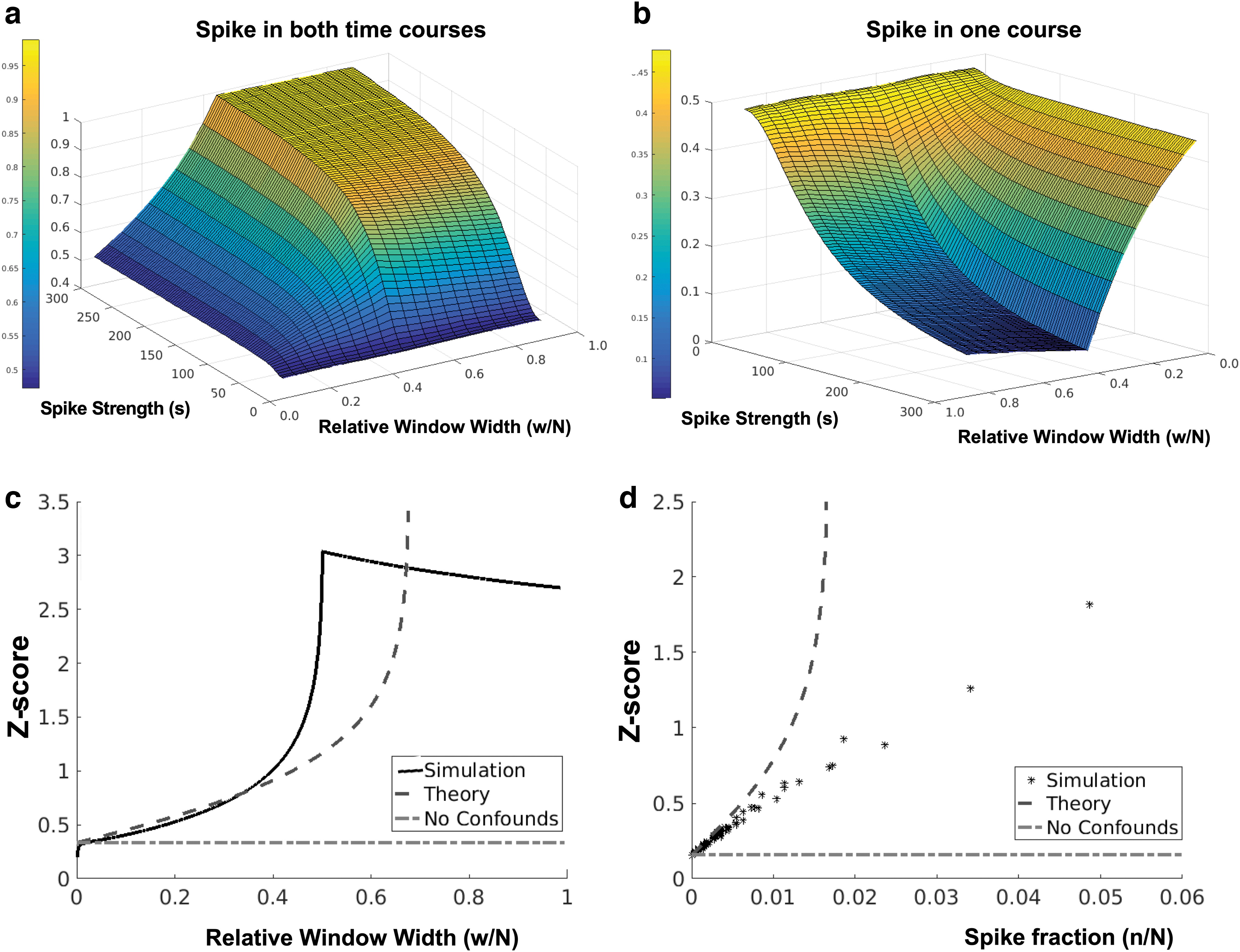
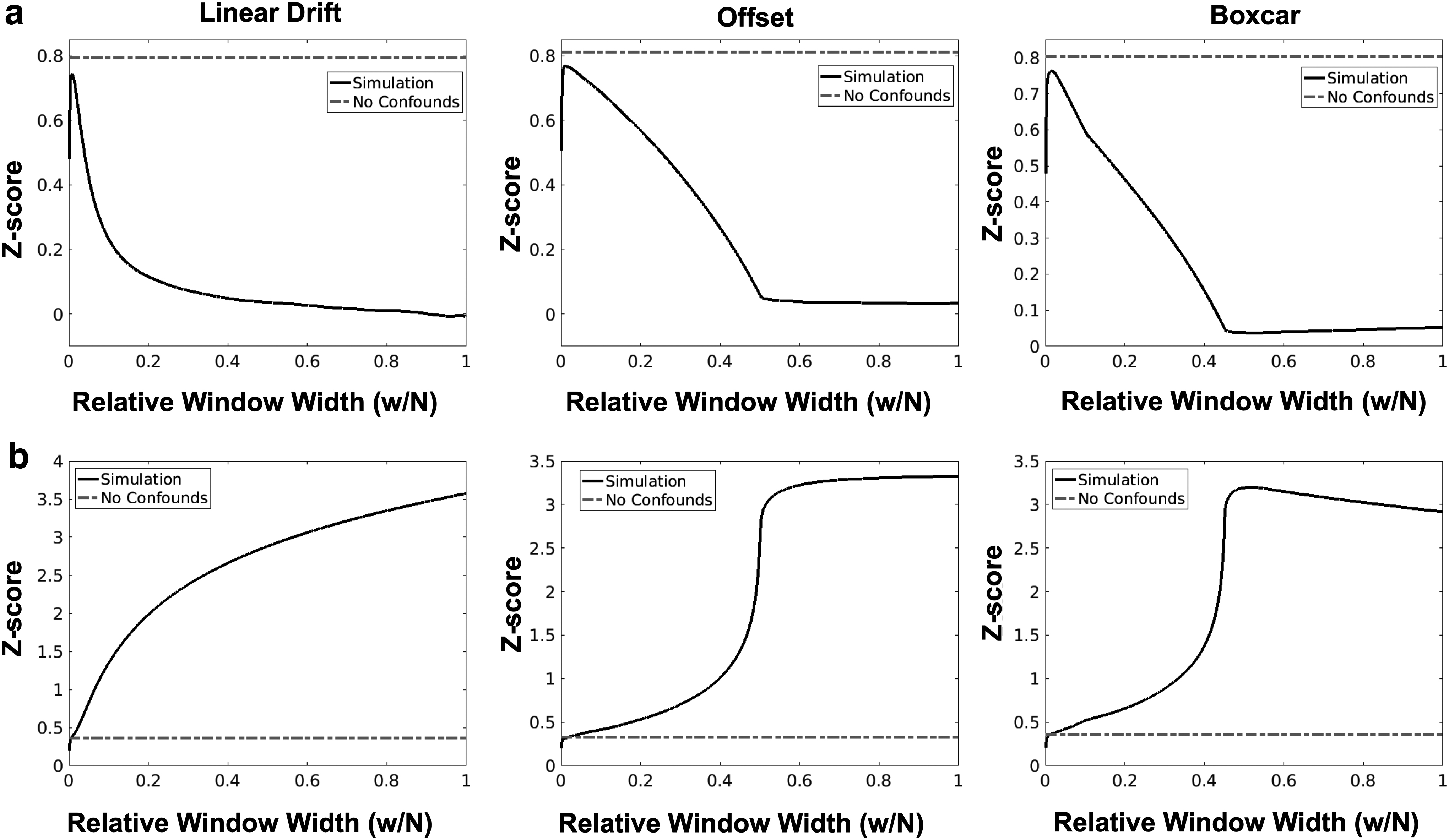
Comparison of analytical and numerical simulations of ASW correlation. A three-dimensional representation of Equation 5 for varying spikes strengths versus relative window width for (a) a spike in both time courses and (b) in single time course. Comparison of the theoretical limit in Equation 6 with numerical simulations: (c) the effect of window width on suppression of a single spike in both time courses. The limit matches well until a relative window width of ∼0.4; (d) the effect of the number of spikes on correlation. The limit matches well until 1% of time points are confounded by spikes. ASW, averaged sliding-window. Color images are available online.

FIG. 3.

Simulation of ASW correlation response to three commonly observed signal confound shapes (drifts, offsets, and boxcars). Signal confounds were simulated in (a) single time course and (b) both time courses. The unconfounded Z-score of the correlation between the original signals is shown with a dashed line in each example. Shorter windows retain original Z-scores. The saturation points seen in the case of offsets are due to the fact that with long enough windows, confounds are sampled by each window rendering the change in width less effective for providing strong confound suppression.

Numerical analysis of ASWR

Figure 4 shows that the removal of confounding signals using averaged partial correlations with sliding-window regression is approximately comparable with ASW correlation after regression across the entire scan, independent of sliding-window width, and with using conventional correlation with regression across the entire scan. Regression is shown to be substantially more effective than ASW correlation without regression, except for short window lengths where ASW correlation itself attenuates the effects of the confounding signals as described above. These simulations assume that the shape of the time course of confounding signals is matched by the shape of the time course of the regression vector. A constant vector was regressed in all cases.

FIG. 4.

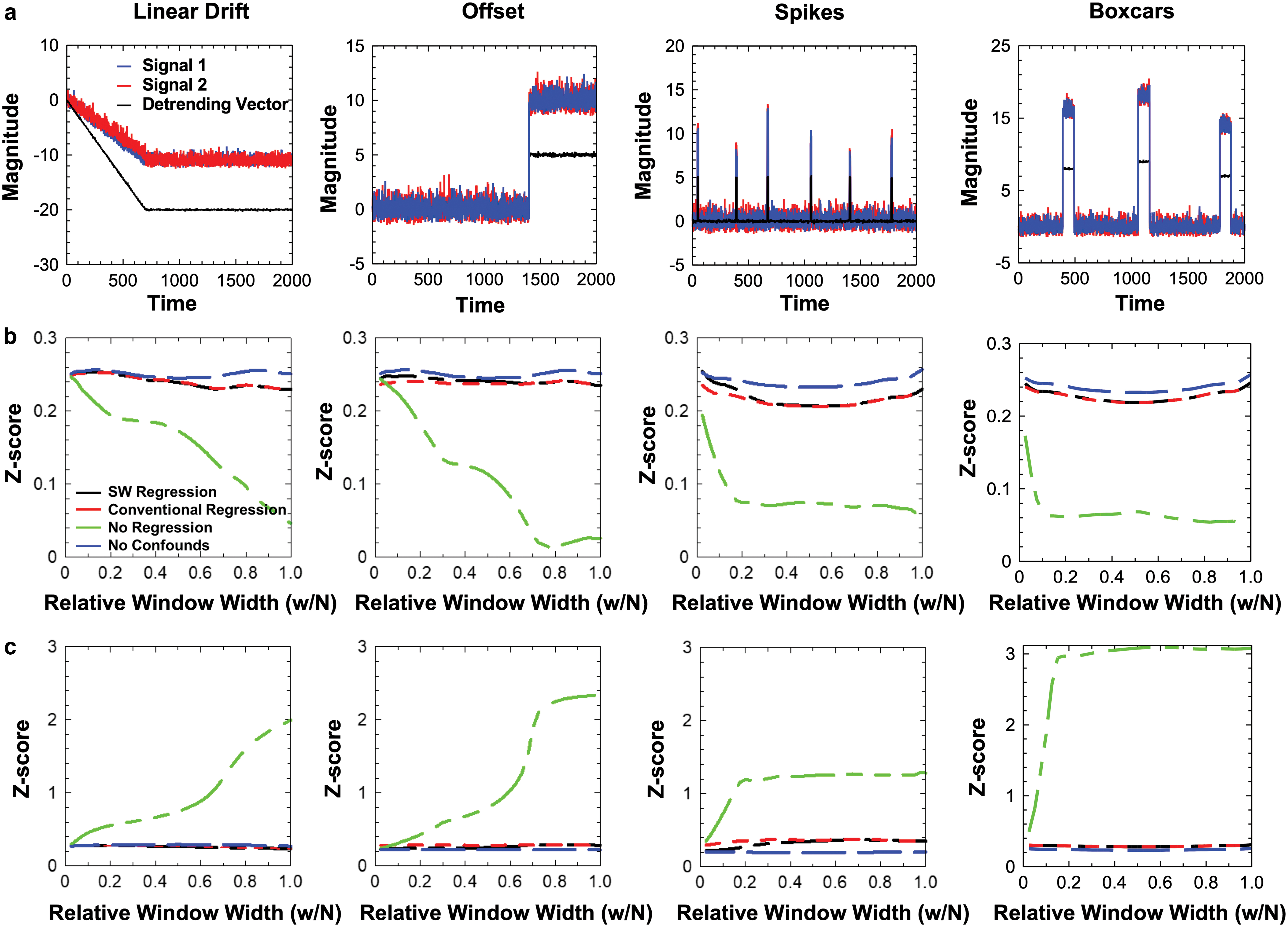
Simulations of ASWR in comparison with conventional regression across the entire time course. (a) Commonly observed confounds were simulated in (b) single and (c) both signal time courses. The Z-scores at the end of the measurement are displayed. Spikes and boxcars were simulated with identical shape and equidistant spacing. The Z-score of the original signals was 0.25. ASWR, averaged sliding-window regression. Color images are available online.

The confound suppression of conventional FWR degrades, in case there is a mismatch between signal confounds and the regression vectors, for example, due to temporal changes of the confound amplitudes that are not reflected in the regression vectors. Neither regression methods completely succeeded to remove the effects of spikes and boxcars in the case where the regression vector did not precisely match the shape of the signal, although at shorter sliding-window widths, sliding-window regression removed confounding signals more efficiently than conventional regression, since the regression coefficients change with window position. Figure 5a and d shows an example of a mismatch in amplitude variation (i.e., shape mismatch) with equidistant spacing between the time courses of the confounding boxcar signal changes and the regression vector where Z-scores with conventional regression across the entire scan and sliding-window regression with long windows deviate substantially from that of the original signals (Fig. 5b, e). Sliding-window correlation more rapidly approaches that of the original signals as window width decreases. For a window width of 12.5% of the full data set, sliding-window regression compensates for the amplitude variations and produces a Z-score time course during sliding-window averaging that is virtually identical to that of the original signals (Fig. 5b, e).

FIG. 5.

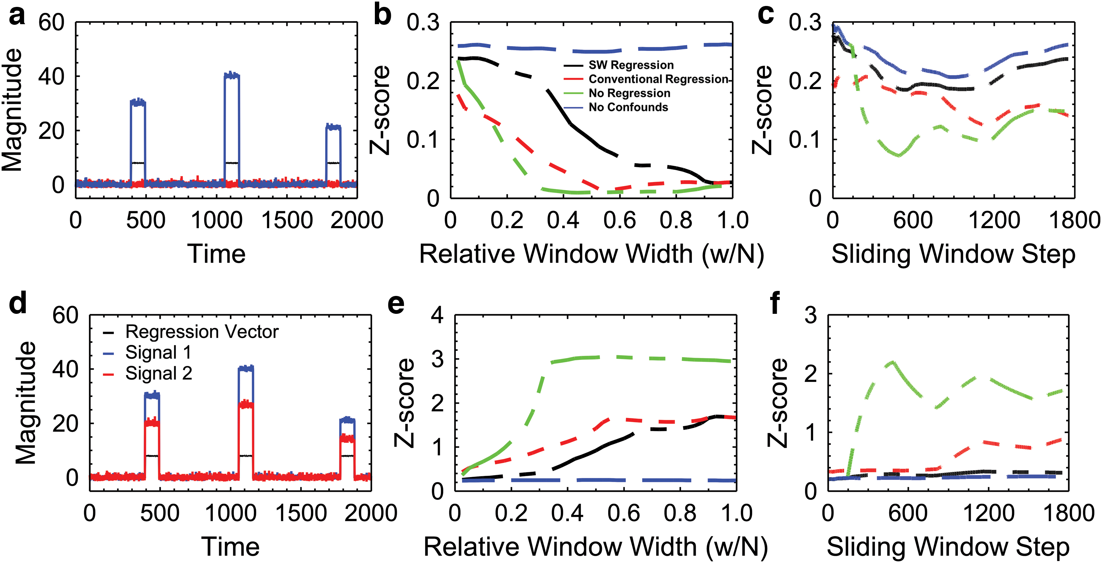
Simulations of ASWR in comparison with conventional regression across the entire time course for the case of a mismatch in amplitude variation (i.e., shape mismatch) with equidistant spacing between (a, d) the confound time courses and the regression vector time course in (a–c) single and (d–f) both the time courses. (b, e) Z-scores at the end of the measurement as a function of window width. (c, f) Temporal evolution of the Z-scores during the measurement for a relative window width of 0.125. Color images are available online.

In vivo validation

The major nodes of SMN, DMN, VSN, and AUN were usually detectable in real time within the 30–60-sec scan duration using both MS-EVI and SMS-EPI, stabilized after 2–3 min, and did not undergo significant changes for the remainder of the scan duration. Most subjects had head movement with linear drifts <2 mm and rotations <2°. False-positive correlation in WM and at slice edges was below a correlation threshold of 0.5 in all subjects.

The high-pass filter characteristics of moving ASW correlation with different sliding-window widths were assessed offline in five subjects scanned using MS-EVI with TR of 136 msec and ASW correlation without regression. Artifactual correlations in WM and in gray matter outside of the major nodes of these networks, in particular in the motion-sensitive frontal cortex, that were detectable when using the zero correlation threshold decreased with decreasing window width and increasing temporal averaging in all subjects (Fig. 6a–e). Correlation coefficients in major nodes decreased with window widths below 15 sec as more strongly correlated low-frequency components below 0.02 Hz were increasingly attenuated due to the high-pass filter characteristics of the sliding-window. Bilateral intranetwork correlations were detected with sliding-window widths as small as 4 sec, suggesting that the frequency range of these networks extends beyond 0.25 Hz, consistent with other studies (Chu et al., 2013; Lee et al., 2013, 2014) and our recent work (Posse et al., 2013; Trapp et al., 2018).

FIG. 6.

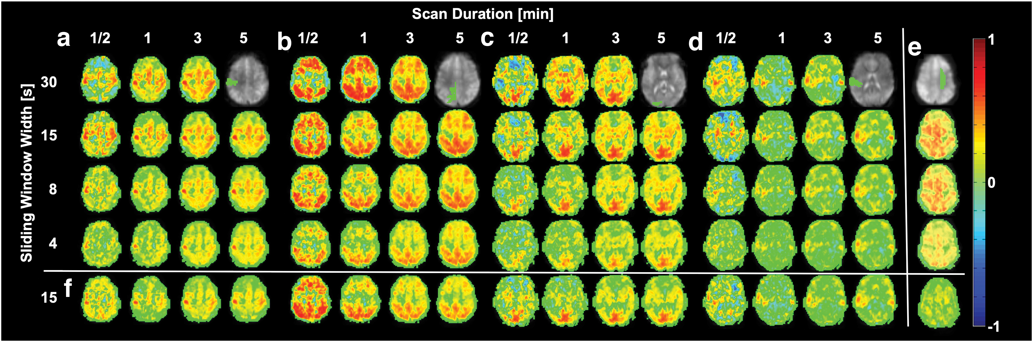
ASW correlation (a–e) without regression as a function of SW width and scan duration, and (f) with regression as a function of scan duration in single-subject MS-EVI data (TR: 136 msec). A representative slice for each of the following seed regions is shown: (a) SMN, (b) DMN, (c) VSN, (d) AUN, and (e) WM. Raw images with the BA seed regions and manually delineated WM seed in green are shown on the top (right) of each subfigure. (f) Addition of regression for an SW width of 15 sec. The meta-mean correlation maps are shown at zero threshold. AUN, auditory network; BA, Brodmann area; DMN, default mode network; MS-EVI, multislab echo-volumar imaging; SMN, sensorimotor network; TR, repetition time; VSN, visual network; WM, white matter. Color images are available online.

Sliding-window regression of motion parameters and signals from WM and CSF was tested offline using MS-EVI data with TR of 136 msec and a sliding-window width of 15 sec to assess the reduction of spatially coherent signal fluctuations between 0.02 and 0.25 Hz. Residual artifactual correlations in WM and in gray matter outside of the major nodes of major networks, including negative correlations in motion-sensitive frontal cortex, which were measured without regression (Fig. 6a–e), decreased when adding sliding-window regression (Fig. 6f).

Group-averaged cluster analysis results using MS-EVI data with TR of 136 msec and resting-state network seeds show a decrease of peak Z scores and spatial extents of correlations (Fig. 7a, b) with decreasing window width and improved suppression of artifactual correlations using regression. Group-averaged cluster analysis results using WM seeds (Fig. 7c, d) show a reduction of the peak Z-scores and spatial extent of artifactual whole-brain correlations with window width and improved suppression of artifactual correlations using regression.

FIG. 7.

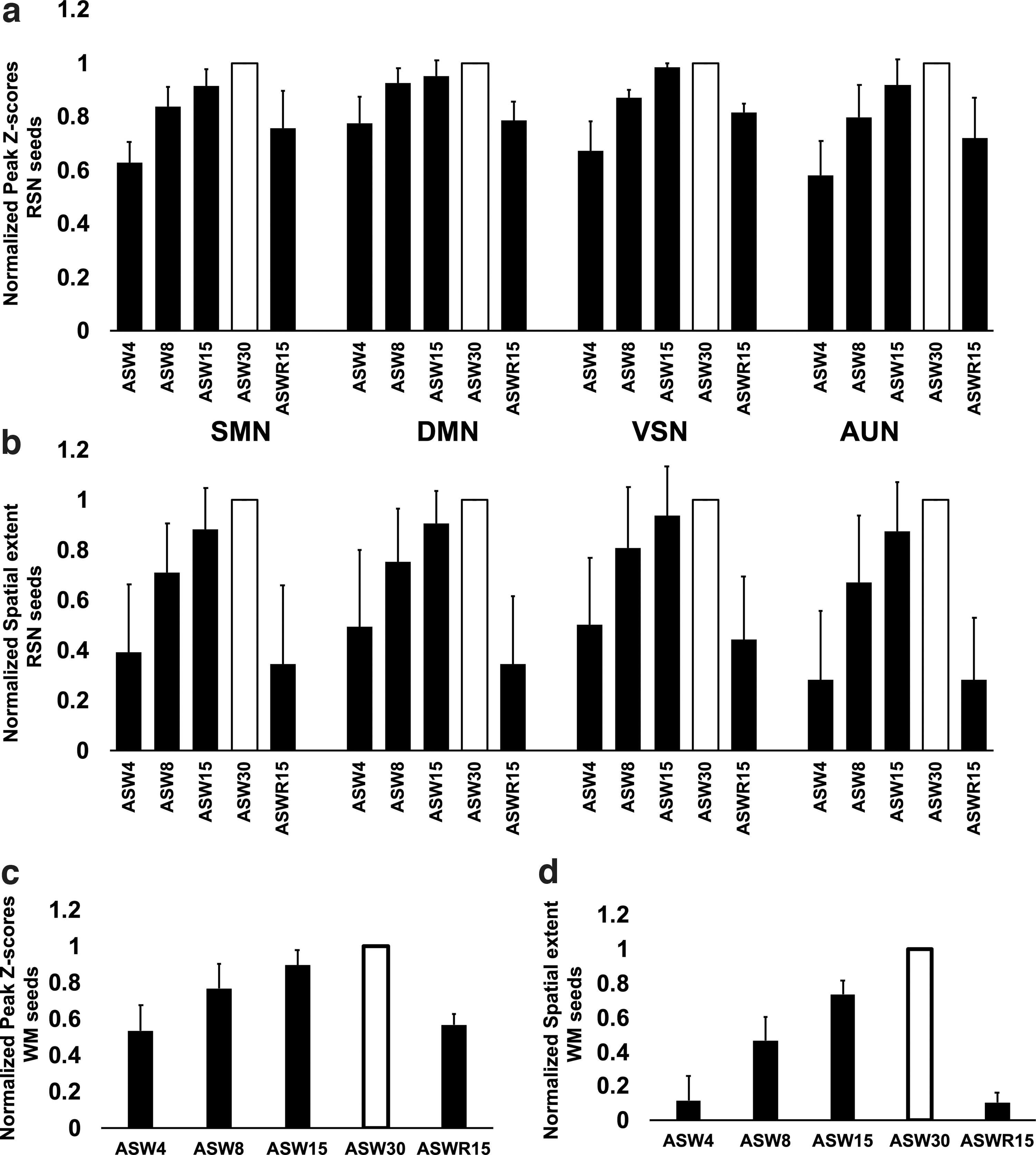
Comparison of ASW correlation without regression (ASW) as a function of SW width (4, 8, 15, and 30 sec), and with regression using an SW width of 15 sec (ASWR15). Group-averaged (N = 5) cluster analysis results in MS-EVI data (TR: 136 msec) at correlation threshold of 0.5 normalized within subject to 30-sec SW without regression (ASW30) showing: (a) normalized peak Fisher Z-transformed correlation values, (b) normalized spatial extents within SMN, DMN, VSN, and AUN, (c) normalized Fisher Z-transformed peak correlation values, and (d) normalized whole-brain spatial extents using WM seeds. The error bars represent the standard deviation across subjects.

A comparison of (1) moving ASW correlation without regression, (2) moving ASW correlation with sliding-window regression, and (3) conventional FWR followed by moving ASW correlation was performed offline in six subjects using SMS-EPI with TR of 400 msec. Residual artifactual correlations in WM and in gray matter outside of the major nodes of SMN, DMN, VSN, and AUN, which were detectable without regression when using a zero-correlation threshold, were strongly reduced in all subjects using both sliding-window and conventional regression (Fig. 8a–d). This reduction of artifactual correlations was particularly evident when using segmented WM masks as seed regions (Fig. 8e). The peak Z-scores within RSNs were comparable between sliding-window and FWR (Fig. 8f, g). The spatial extent of connectivity with sliding-window regression was ∼50% of that with FWR when averaged across networks. Across all subjects, the reduction of artifactual correlations using sliding-window regression was comparable with that using conventional FWR across the entire scan (Fig. 8h), with minor regional differences that likely reflect differences between the regression based on Equation 7 implemented in TurboFIRE and the PCA-based regression using MATLAB tools.

FIG. 8.

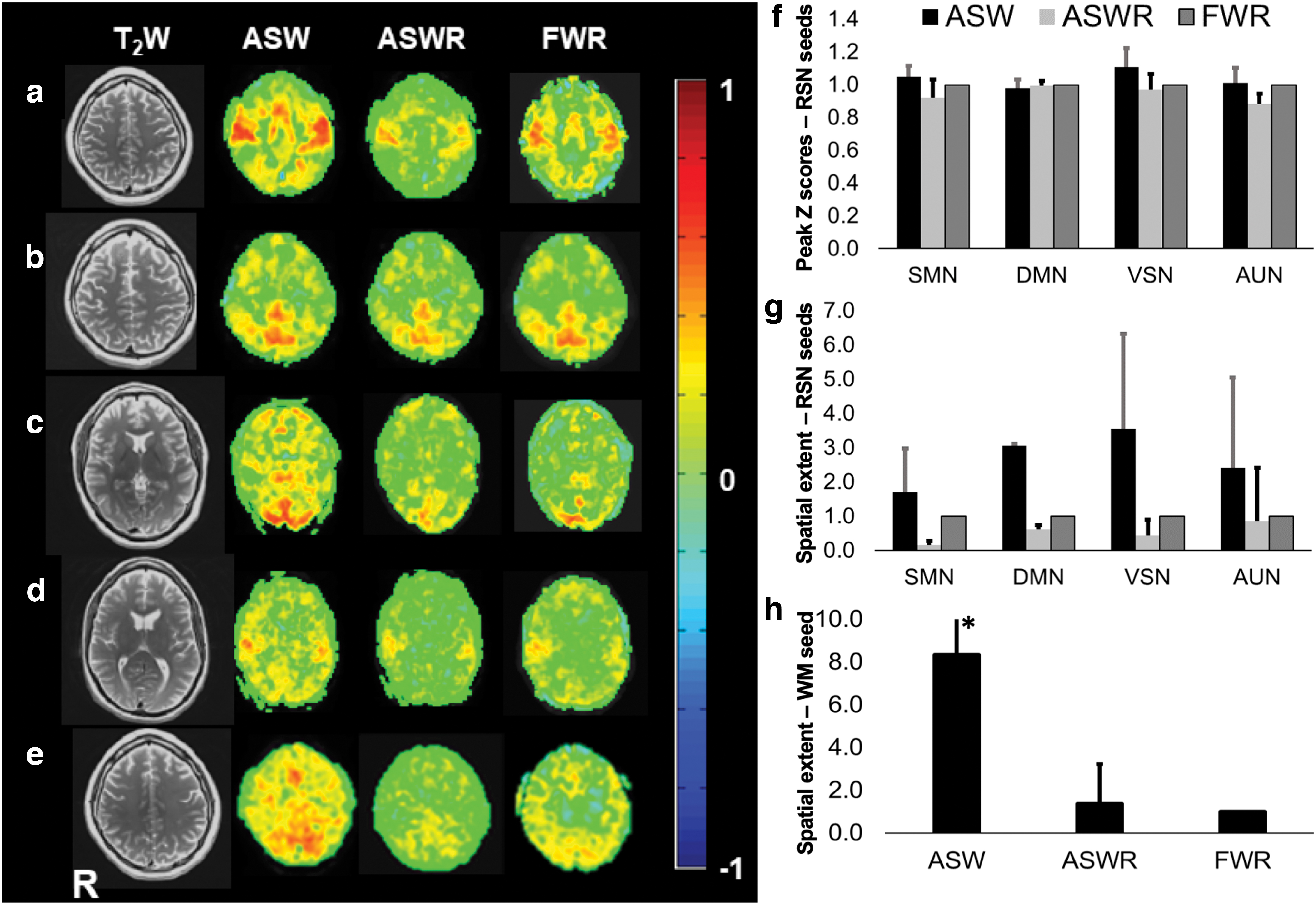
Comparison of resting-state correlations in single-subject SMS-EPI data (TR: 400 msec) using ASW, ASWR, and FWR with seeds in (a) SMN, (b) DMN, (c) VSN, (d) AUN, and (e) using segmented WM masks as seed regions. The meta-mean correlation maps are shown at zero threshold. Group-averaged (N = 6) cluster analysis results at correlation threshold of 0.5 normalized within subject to FWR showing (f) normalized peak Fisher Z-transformed correlations in resting-state networks, (g) normalized spatial extents within resting-state network seed regions, and (h) normalized whole-brain spatial extent using WM seed. The error bars represent the standard deviation across subjects. *Error bar (11.7) off-scale. FWR, full window regression; SMS-EPI, simultaneous multislice echo-planar imaging. Color images are available online.

Computational performance

The image reconstruction and transfer of each image took <1 TR for all pulse sequences in this study. Steady-state preprocessing of a 32-slice SMS-EPI data set with 64 × 64 matrix, including motion correction and spatial and temporal filtering, took ∼100 msec per image using a single thread. Steady-state, sliding-window correlation of four ROIs with regression of 6 motion parameters, WM and CSF signals using 64 threads took ∼200 msec per image. Steady-state postprocessing including moving averaging of sliding-window correlation maps took ∼10 msec per image. The time required for resampling and displaying imaging and ROI time course data in the graphical user interface (GUI) was dependent on the size of the GUI on the monitor (3840 × 2160 pixels) and ranged from 50 msec per image for a 900 × 570 pixel GUI to 210 msec per image for a 2300 × 1400 pixel GUI. SMS-EPI data acquired with TR: 400 msec could be processed in near-steady state using two seed regions and sliding-window regression (Fig. 9). Time delays up to 20% after the end of the scans were encountered using four seed regions and sliding-window regression. Larger time delays ranging from 47% to 157% after the end of the scan depending on the processing method and number of seeds were measured using MS-EVI data acquired with TR: 136 msec.

FIG. 9.

Computational performance of the real-time, resting-state fMRI analysis pipeline on a 36-core Linux workstation. The steady-state processing time per image for ASW and ASWR was computed as a function of the number of seeds using MS-EVI (TR: 136 msec, spatial matrix: 64 × 64, no. of slices: 16) and SMS-EPI (TR: 400 msec, spatial matrix: 64 × 64, no. of slices: 32) data. fMRI, functional magnetic resonance imaging.

An actual real-time fMRI experiment required a prescan to acquire an image volume for spatial normalization, atlas-based seed selection, and manual delineation of WM and CSF regions in case of regression. The preparation time, including prescan before the actual real-time scan, was 1–2 min without sliding-window regression and 4–8 min with sliding-window regression, depending on the number of seed regions.

Resting-state network connectivity dynamics and internetwork connectivity

An example of monitoring intra- and internetwork temporal dynamics using the second-level sliding-window approach is shown in Figure 10. All mapped resting-state networks stabilized after the first minute of the scan and retained the initial spatial pattern across the scan (Fig. 10a–d). Figure 10e shows 12 × 12 matrices of interseed correlations that monitor the stabilization of intranetwork correlations within 12 seed regions during the scan. The corresponding cluster results show that spatial extents, peak correlations, mean correlations, and the SD of correlations within the clusters stabilized after the initial 1–1.5 min of the scan (Fig. 10f–i).

FIG. 10.

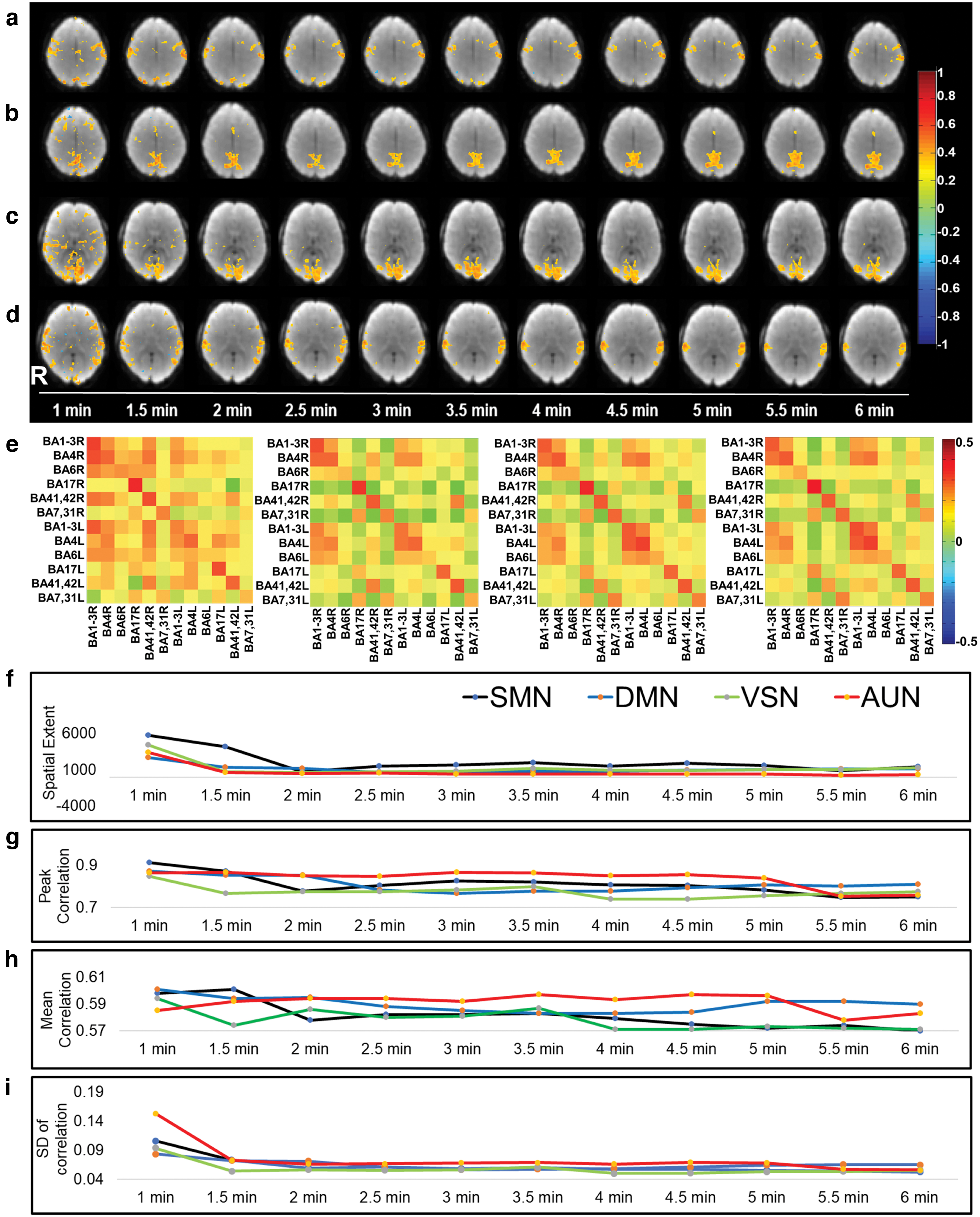
Temporal dynamics of resting-state connectivity at half-minute intervals in (a) SMN, (b) DMN, (c) VSN, and (d) AUN with first- and second-level SWs (W ₁ = 8 sec, W ₂ = 30 sec) using SMS-EPI data (TR: 400 msec). The peak clusters of the resting-state connectivity are monitored across a 6-min scan using (e) the 12 × 12 intra- and inter-resting-state network correlation matrices representing the connectivity dynamics at 1-, 3-, 5-, and 6-min scan intervals, which are dominated by bilateral intra-SMN connectivity (labels represent the left and right BA seeds for SMN, DMN, VSN, and AUN), and the (f) spatial extent (no. of voxels), (g) peak and (h) mean correlation, and (i) standard deviation of the correlation within the clusters. The correlation maps in (a–d) are shown at a correlation threshold of 0.5. The color contrast in (e) was enhanced using a correlation scale from −0.5 (blue) to 0.5 (red). Color images are available online.

Moving averaged correlation analysis with 15-sec sliding-window enabled mapping of 28 resting-state networks in single subjects using MS-EVI with TR of 136 msec. Single-subject, internetwork correlation matrices (Fig. 11a) displayed stronger anticorrelations across the DMN and VSN nodes than the internetwork correlation matrix averaged across five subjects (Fig. 11b). The group-averaged internetwork correlation matrix displayed predominantly positive correlations that have similarity with the connectivity patterns of the functional network connectivity matrix (FNCM) presented in Allen et al. (2011). The strongest correlations (blocks of high connectivity across the principal diagonal) are seen within the seven classes of resting-state networks, both in the single subjects and in group results, a characteristic feature also observed in the FNCM presented in Allen et al. (2011). The sensorimotor seed shows strong positive correlations with the attention seed and weaker correlations with the visual seed. The default mode ROI is less strongly correlated with the rest of task-positive resting-state network seeds, as expected.

FIG. 11.

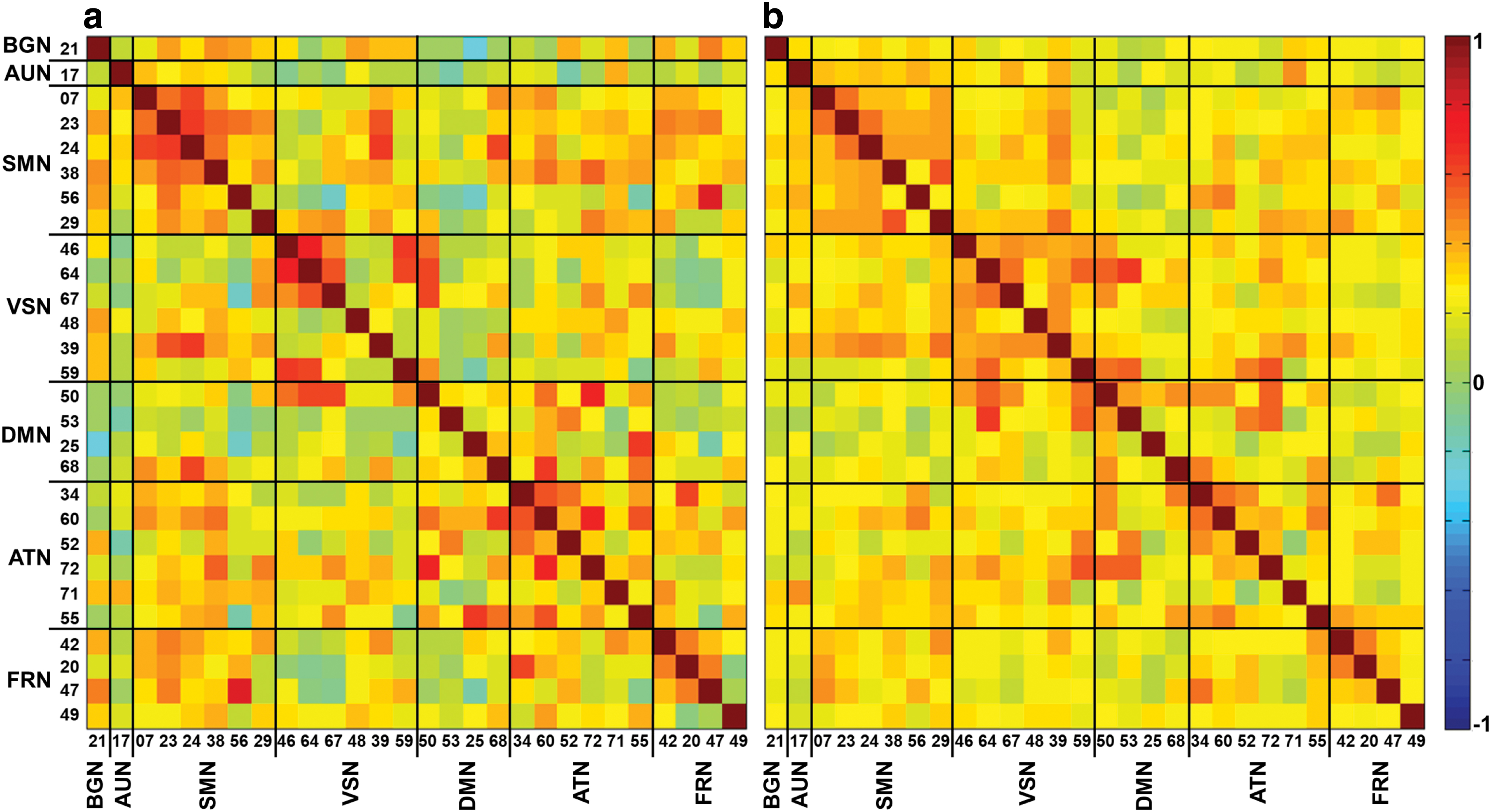
Single-subject (a) and group-averaged (b) internetwork correlation matrices between 28 seed regions computed at zero meta-mean correlation threshold using MS-EVI data (TR: 136 msec) measured in 5 subjects. The seed regions were selected based on the following network nodes and ICA components described in Allen et al. (2011): attention—IC34, IC52, IC55, IC60, IC71, IC72; auditory—IC17; basal ganglia—IC21; default mode—IC25, IC50, IC53, IC68; frontal—IC20, IC42, IC47, IC49; sensorimotor—IC07, IC23, IC24, IC29, IC38, IC56; and visual—IC39, IC46, IC48, IC59, IC64, IC67. ATN, attention network; BGN, basal ganglia network; FRN, frontal network; IC, independent component; ICA, independent component analysis. Color images are available online.

Discussion

The present study introduces a computationally efficient real-time, seed-based, resting-state fMRI analysis pipeline using moving ASW partial correlations with regression of confounding signals from motion, WM, and CSF. We show that ASW correlation per se provides confound tolerance that increases with decreasing window width. When adding sliding-window regression, the suppression of confounding signal correlations becomes comparable with that of offline FWR. In situations where there is a mismatch between the regression vector and the confounding signals, confound suppression of sliding-window regression may even surpass that of FWR. The methodology is suitable for real-time, seed-based, resting-state fMRI analysis with very short TR that allows unaliased sampling of cardiac-related signal pulsation. The study also introduces a second-level sliding-window approach that is suitable for monitoring intra- and internetwork correlation dynamics while maintaining confound tolerance and demonstrated the feasibility of mapping internetwork correlations.

Suppression of artifactual connectivity

Our analytical and numerical analyses and in vivo data in the current and our previous study (Posse et al., 2013) show that ASW correlation without regression of confounding signals already provides considerable confound suppression. ASW correlation reduces the effects of isolated signal changes such as spikes. Traditional despiking methods (Cox, 1996; Gold et al., 1998) provide stronger spike suppression, but require the ability to reliably identify isolated signal events and do not account for more complex confound waveforms. Moving ASW correlation does not require a priori knowledge of signal characteristics and is particularly advantageous for mapping high-frequency connectivity where artifact characteristics are less well established, and the high degree of averaging using short windows enhances confound suppression as our recent study has demonstrated (Trapp et al., 2018). The addition of sliding-window regression further enhanced confound suppression in vivo to a level that was comparable with and in some data sets even surpassed the performance of conventional FWR. Inspection of these data revealed that there were shape discrepancies between the confounding signals and the regression vectors, in particular in frontal brain regions that are sensitive to motion artifacts.

Frequency selectivity of sliding-windows

The ASW approach provides a selectable trade-off between the degrees of confound suppression and the high-pass filtering frequency cutoff, which both increase with decreasing window width. The range of sliding-window widths used in this study (4–30 sec) in conjunction with a 4- or 8-sec Hamming-windowed MAF creates a bandpass with a low-frequency cutoff of 0.005–0.02 Hz and a high-frequency cutoff of 0.25–0.5 Hz at −30 dB attenuation, which is consistent with the frequency spectrum of resting-state fluctuations. A 15-sec sliding-window was the preferred window to capture resting-state fluctuations above ∼0.02 Hz (−20 dB attenuation), which is roughly consistent with the rule-of-thumb criterion “window width (W) ≥ 1/f _min” described in Leonardi and Van De Ville (2015). However, we also detected functional connectivity at much shorter window widths at correspondingly reduced sensitivities, similar to Zalesky and Breakspear (2015). The AUN, SMN, and VSN exhibit considerable high-frequency connectivity (0.3–0.5 Hz), which was detected using sliding-windows as short as 4 sec.

Limitations

This study provides a preliminary assessment of the performance of our analysis pipeline in vivo. A larger scale study is required to compare the sensitivity and specificity of mapping resting-state networks with state-of-the-art resting-state analysis pipelines. A correction of the correlation thresholds for the degrees of freedom as a function of sliding-window width has not been applied in the present study and is under investigation. Regression analysis assumes that the regressors and the underlying resting-state signal fluctuation time courses are orthogonal (e.g., Monti, 2011; Mumford et al., 2015). Collinearity between the regressors and the resting-state signal fluctuations, which could not be excluded in our approach, may have decreased the measured correlations. Integration of real-time, PCA-based extraction of regressors (e.g., using CompCor; Behzadi et al., 2007) will be the subject of a future study. Seed-based approaches are highly sensitive to the choice of the seed locations, and therefore, seeds were carefully chosen, particularly in MS-EVI data sets to avoid slab edges, where respiratory artifacts primarily manifest. Seed optimization tailored to individual anatomy along with robust spatial normalization techniques in real time is currently under investigation.

Conclusions

This computationally efficient and confound-tolerant, seed-based, resting-state fMRI analysis approach using moving ASW with partial correlations and regression of confounding signal changes provides a flexible framework for mapping resting-state connectivity in single subjects in real time and probing temporal dynamics of whole-brain connectivity at timescales as short as 30 sec. This approach is particularly suitable for real-time mapping of resting-state connectivity using high-speed fMRI, single-subject analyses, monitoring data quality, and clinical applications, such as presurgical mapping (Posse et al., 2013; Vakamudi et al., 2020).

Software Distribution

A custom MATLAB toolbox to simulate and process signal time courses to characterize signal correlations using sliding-window correlation analysis with sliding-window regression.

Footnotes

Authors' Contributions

K.V.: conducted software performance checks, recruited subjects, and processed data. C.T.: developed simulation software in MATLAB to characterize moving average sliding-window correlation and MAFs. K.T.: developed simulation software in MATLAB to characterize sliding-window regression in combination with moving average sliding-window correlation and MAFs. K.G.: designed the parallel architecture and implemented the analysis pipeline in C++ in the TurboFIRE software package. B.R.G.: processed data. S.P.: conceived and coordinated the study, defined software architecture and functionality, conducted software performance checks, and acquired, processed, and interpreted the study data. K.V., C.T., K.T., and S.P.: wrote the article.

Acknowledgments

We gratefully acknowledge our former laboratory member Elena S. Ackley for her original contributions to developing the TurboFIRE software and moving ASW correlations. We wish to thank the following people for their contributions to this work: Arvind Caprihan, PhD, for advice on signal modeling, Eswar Damaraju for his help with the implementation of a PCA-based FWR preprocessing pipeline, Vince D. Calhoun, PhD, for providing valuable feedback on the measurement of resting-state connectivity with ICA and seed-based methods, Orrin Myers, PhD, for his suggestions regarding statistical analyses, Joel Castellanos, PhD, and Robin Campos for help with optimizing intra- and inter-resting-state network correlation matrices in TurboFIRE, Diana South and Catherine Smith for their assistance with scanner operations, Greg Scantlen for supporting TurboFIRE testing on high-performance workstations, and Jan Minterovitch, PhD, and Dieter Dennig, MD, PhD, for their project support. We sincerely thank our subjects for their participation in this study.

Author Disclosure Statement

The corresponding author is the founder of NeurInsight, LLC that developed components of the TurboFIRE software tool with STTR funding (1R41NS090691). The coauthors declare no competing financial conflicts of interest.

Funding Information

The corresponding author received funding from the National Institutes of Health (grants 1R21EB022803, 1R41NS090691, 1R21EB018494, 1P30GM122734, and 2P20GM103472).

References

Allen

, Erhardt

, Damaraju

, Gruner

, Segall

, Silva

, et al. 2011. A baseline for the multivariate comparison of resting-state networks. Front Syst Neurosci, 5:2.

Behzadi

, Restom

, Liau

, Liu

. 2007. A component based noise correction method (CompCor) for BOLD and perfusion based fMRI. Neuroimage, 37:90–101.

Chu

, Ahveninen

, Tommi

, Kuo

W-J

, Belliveau

, Lin

F-H

. Resting-state fMRI at 4 Hz. In Annual Meeting of the ISMRM, Salt Lake City, USA, Abstract 41, 2013.

Cox

RW.

1996. AFNI: software for analysis and visualization of functional magnetic resonance neuroimages. Comput Biomed Res, 29:162–173.

D'Esposito

2019. Are individual differences in human brain organization measured with functional MRI meaningful?. Proc Natl Acad Sci U S A, 116:22432–22434.

Dosenbach

NUF

, Koller

, Earl

, Miranda-Dominguez

, Klein

, Van

, et al. 2017. Real-time motion analytics during brain MRI improve data quality and reduce costs. Neuroimage, 161:80–93.

Esposito

, Seifritz

, Formisano

, Morrone

, Scarabino

, Tedeschi

, et al. 2003. Real-time independent component analysis of fMRI time-series. Neuroimage, 20:2209–2224.

Feinberg

, Moeller

, Smith

, Auerbach

, Ramanna

, Gunther

, et al. 2010. Multiplexed echo planar imaging for sub-second whole brain FMRI and fast diffusion imaging. PLoS One, 5:e15710.

Gao

, Posse

. TurboFire: real-time fMRI with automated spatial normalization and Talairach Daemon database. In Proceedings of the 9th Annual Meeting of the Organization of Human Brain Mapping, Budapest, Hungary, 2003, p. 838.

10.

Gao

, Posse

. TurboFIRE: real-time fMRI with online generation of reference vectors. In Proceedings of the 10th Annual Meeting of the Organization of Human Brain Mapping, Budapest, Hungary, 2004, WE177.

11.

Gembris

, Taylor

, Schor

, Frings

, Suter

, Posse

. 2000. Functional magnetic resonance imaging in real time (FIRE): sliding-window correlation analysis and reference-vector optimization. Magn Reson Med, 43:259–268.

12.

Glover

, Li

, Ress

. 2000. Image-based method for retrospective correction of physiological motion effects in fMRI: RETROICOR. Magn Reson Med, 44:162–167.

13.

Gold

, Christian

, Arndt

, Zeien

, Cizadlo

, Johnson

, et al. 1998. Functional MRI statistical software packages: a comparative analysis. Hum Brain Mapp, 6:73–84.

14.

Gordon

, Laumann

, Adeyemo

, Gilmore

, Nelson

, Dosenbach

NUF

, Petersen

. 2017. Individual-specific features of brain systems identified with resting state functional correlations. Neuroimage, 146:918–939.

15.

Kim

, Yoo

, Tegethoff

, Meinlschmidt

, Lee

. 2015. The inclusion of functional connectivity information into fMRI-based neurofeedback improves its efficacy in the reduction of cigarette cravings. J Cogn Neurosci, 27:1552–1572.

16.

Koush

, Ashburner

, Prilepin

, Sladky

, Zeidman

, Bibikov

, et al. 2017. OpenNFT: an open-source Python/MATLAB framework for real-time fMRI neurofeedback training based on activity, connectivity and multivariate pattern analysis. Neuroimage, 156:489–503.

17.

Koush

, Rosa

, Robineau

, Heinen

, Rieger

, Weiskopf

, et al. 2013. Connectivity-based neurofeedback: dynamic causal modeling for real-time fMRI. Neuroimage, 81:422–430.

18.

Lancaster

, Woldorff

, Parsons

, Liotti

, Freitas

, Rainey

, et al. 2000. Automated Talairach atlas labels for functional brain mapping. Hum Brain Mapp, 10:120–131.

19.

Lee

, Asslander

, LeVan

, Hennig

. Resting-state functional hubs at multiple frequencies revealed by MR-encephalography. In Proceedings of the International Society for Magnetic Resonance in Medicine, International Society for Magnetic Resonance in Medicine, Milan, 2014, p. 4184.

20.

Lee

, Zahneisen

, Hugger

, LeVan

, Hennig

. 2013. Tracking dynamic resting-state networks at higher frequencies using MR-encephalography. Neuroimage, 65:216–222.

21.

Leonardi

, Van De Ville

. 2015. On spurious and real fluctuations of dynamic functional connectivity during rest. Neuroimage, 104:430–436.

22.

Lin

, Nummenmaa

, Witzel

, Polimeni

, Zeffiro

, Wang

, Belliveau

. 2012. Physiological noise reduction using volumetric functional magnetic resonance inverse imaging. Hum Brain Mapp, 33:2815–2830.

23.

Liu

TT.

2016. Noise contributions to the fMRI signal: an overview. Neuroimage, 143:141–151.

24.

Margulies

, Bottger

, Long

, Lv

, Kelly

, Schafer

, et al. 2010. Resting developments: a review of fMRI post-processing methodologies for spontaneous brain activity. MAGMA, 23:289–307.

25.

Megumi

, Yamashita

, Kawato

, Imamizu

. 2015. Functional MRI neurofeedback training on connectivity between two regions induces long-lasting changes in intrinsic functional network. Front Hum Neurosci, 9:160.

26.

Misaki

, Barzigar

, Zotev

, Phillips

, Cheng

, Bodurka

. 2015. Real-time fMRI processing with physiological noise correction—comparison with off-line analysis. J Neurosci Methods, 256:117–121.

27.

Misaki

, Phillips

, Zotev

, Wong

, Wurfel

, Krueger

, et al. 2018. Real-time fMRI amygdala neurofeedback positive emotional training normalized resting-state functional connectivity in combat veterans with and without PTSD: a connectome-wide investigation. Neuroimage Clin, 20:543–555.

28.

Monti

MM.

2011. Statistical analysis of fMRI time-series: a critical review of the GLM approach. Front Hum Neurosci, 5:28.

29.

Monti

, Lorenz

, Braga

, Anagnostopoulos

, Leech

, Montana

2017. Real-time estimation of dynamic functional connectivity networks. Hum Brain Mapp, 38:202–220.

30.

Mumford

, Poline

, Poldrack

. 2015. Orthogonalization of regressors in FMRI models. PLoS One, 10:e0126255.

31.

Muschelli

, Nebel

, Caffo

, Barber

, Pekar

, Mostofsky

. 2014. Reduction of motion-related artifacts in resting state fMRI using aCompCor. Neuroimage, 96:22–35.

32.

Posse

, Ackley

, Mutihac

, Rick

, Shane

, Murray-Krezan

, et al. 2012. Enhancement of temporal resolution and BOLD sensitivity in real-time fMRI using multi-slab echo-volumar imaging. Neuroimage, 61:115–130.

33.

Posse

, Ackley

, Mutihac

, Zhang

, Hummatov

, Akhtari

, et al. 2013. High-speed real-time resting-state FMRI using multi-slab echo-volumar imaging. Front Hum Neurosci, 7:479.

34.

Posse

, Wiese

, Gembris

, Mathiak

, Kessler

, Grosse-Ruyken

, et al. 1999. Enhancement of BOLD-contrast sensitivity by single-shot multi-echo functional MR imaging. Magn Reson Med, 42:87–97.

35.

Satterthwaite

, Elliott

, Gerraty

, Ruparel

, Loughead

, Calkins

, et al. 2013. An improved framework for confound regression and filtering for control of motion artifact in the preprocessing of resting-state functional connectivity data. Neuroimage, 64:240–256.

36.

Satterthwaite

, Wolf

, Loughead

, Ruparel

, Elliott

, Hakonarson

, et al. 2012. Impact of in-scanner head motion on multiple measures of functional connectivity: relevance for studies of neurodevelopment in youth. Neuroimage, 60:623–632.

37.

Setsompop

, Gagoski

, Polimeni

, Witzel

, Wedeen

, Wald

. 2012. Blipped-controlled aliasing in parallel imaging for simultaneous multislice echo planar imaging with reduced g-factor penalty. Magn Reson Med, 67:1210–1224.

38.

Smith

, Beckmann

, Andersson

, Auerbach

, Bijsterbosch

, Douaud

, et al. 2013. Resting-state fMRI in the Human Connectome Project. Neuroimage, 80:144–168.

39.

Soldati

, Calhoun

, Bruzzone

, Jovicich

. 2013a. ICA analysis of fMRI with real-time constraints: an evaluation of fast detection performance as function of algorithms, parameters and a priori conditions. Front Hum Neurosci, 7:19.

40.

Soldati

, Calhoun

, Bruzzone

, Jovicich

. 2013b. The use of a priori information in ICA-based techniques for real-time fMRI: an evaluation of static/dynamic and spatial/temporal characteristics. Front Hum Neurosci, 7:64.

41.

Trapp

, Vakamudi

, Posse

. 2018. On the detection of high frequency correlations in resting state fMRI. Neuroimage, 164:202–213.

42.

Triantafyllou

, Polimeni

, Wald

. 2011. Physiological noise and signal-to-noise ratio in fMRI with multi-channel array coils. Neuroimage, 55:597–606.

43.

Vakamudi

, Posse

, Jung

, Cushnyr

, Chohan

. 2020. Real-time presurgical resting-state fMRI in patients with brain tumors: quality control and comparison with task-fMRI and intraoperative mapping. Hum Brain Mapp, 41:797–814.

44.

Van Dijk

, Sabuncu

, Buckner

. 2012. The influence of head motion on intrinsic functional connectivity MRI. Neuroimage, 59:431–438.

45.

Welford

BP.

1962. Note on method calculating correct sum of squares and products. Technometrics, 4:419–420.

46.

Young

, Siegle

, Misaki

, Zotev

, Phillips

, Drevets

, Bodurka

. 2018. Altered task-based and resting-state amygdala functional connectivity following real-time fMRI amygdala neurofeedback training in major depressive disorder. Neuroimage Clin, 17:691–703.

47.

Zahneisen

, Grotz

, Lee

, Ohlendorf

, Reisert

, Zaitsev

, Hennig

. 2011. Three-dimensional MR-encephalography: fast volumetric brain imaging using rosette trajectories. Magn Reson Med, 65:1260–1268.

48.

Zalesky

, Breakspear

. 2015. Towards a statistical test for functional connectivity dynamics. Neuroimage, 114:466–470.

49.

Zilverstand

, Sorger

, Zimmermann

, Kaas

, Goebel

. 2014. Windowed correlation: a suitable tool for providing dynamic fMRI-based functional connectivity neurofeedback on task difficulty. PLoS One, 9:e85929.