Understanding Global Brain Network Alterations in Glioma Patients

Abstract

Introduction:

Glioma patients show increased global brain network clustering related to poorer cognition and epilepsy. However, it is unclear whether this increase is spatially widespread, localized in the (peri)tumor region only, or decreases with distance from the tumor.

Materials and Methods:

Weighted global and local brain network clustering was determined in 71 glioma patients and 53 controls by using magnetoencephalography. Tumor clustering was determined by averaging local clustering of regions overlapping with the tumor, and vice versa for non-tumor regions. Euclidean distance was determined from the tumor centroid to the centroids of other regions.

Results:

Patients showed higher global clustering compared with controls. Clustering of tumor and non-tumor regions did not differ, and local clustering was not associated with distance from the tumor. Post hoc analyses revealed that in the patient group, tumors were located more often in regions with higher clustering in controls, but it seemed that tumors of patients with high global clustering were located more often in regions with lower clustering in controls.

Conclusions:

Glioma patients show non-local network disturbances. Tumors of patients with high global clustering may have a preferred localization, namely regions with lower clustering in controls, suggesting that tumor localization relates to the extent of network disruption.

Impact statement

This work uses the innovative framework of network neuroscience to investigate functional connectivity patterns associated with brain tumors. Glioma (primary brain tumor) patients experience cognitive deficits and epileptic seizures, which have been related to brain network alterations. This study shows that glioma patients have a spatially widespread increase in global network clustering, which cannot be attributed to local effects of the tumor. Moreover, tumors occur more often in brain regions with higher network clustering in controls. This study emphasizes the global character of network alterations in glioma patients and suggests that preferred tumor locations are characterized by particular network profiles.

Introduction

Gliomas are the most frequently diagnosed primary brain tumors and are characterized by poor prognosis. Overall survival ranges from months to several years depending on tumor subtype (Ho et al., 2014). Patients may experience a wide range of neurological and cognitive deficits, and valuable insights in these tumor-related sequelae have been obtained through graph theoretical analyses (Aerts et al., 2016; Derks et al., 2014).

Widespread deviations from the healthy brain network have been demonstrated in studies using magnetoencephalography (MEG) to establish the functional brain network in glioma patients, particularly showing higher global network clustering (Bosma et al., 2009; Derks et al., 2014; Fox and King, 2018; van Dellen et al., 2012; Wang et al., 2010). These differences are associated with poorer cognitive functioning and greater frequency or longer duration of epilepsy (van Dellen et al., 2012; Wang and Meng, 2016). Global network clustering is often calculated as the average of all local clustering coefficients and labels the extent to which neighboring brain regions are also connected in terms of number or weight of connections (Watts and Strogatz, 1998). The “pathological” clustering in glioma patients is mostly seen in the theta (4–8 Hz) frequency band (Bosma et al., 2009; van Dellen et al., 2012).

However, previous studies did not distinguish between global and local increases in functional network clustering. Hypothetically, increased average network clustering could reflect either (1) a non-local and widespread increase in clustering, (2) a specific increase in clustering in only the tumor region (e.g., local clustering) that raises the average clustering, or (3) a more gradual distribution of high clustering around the tumor that decays at further distance from the tumor. Greater understanding of the properties of pathological clustering may aid in improved prognostication of cognitive decline in these patients and may help delineate potential future treatment options for these patients.

In this study, brain networks derived from MEG recordings of glioma patients were analyzed. Global clustering was compared between patients and matched healthy controls (HCs), and local clustering of tumor regions and regions without tumor were computed. The Euclidean distance between the tumor area and all other brain regions was used to investigate the relationship between distance from the tumor and local clustering.

Materials and Methods

Patients

Patients with suspected diffuse glioma who visited the Amsterdam University Medical Center between 2010 and 2017, and age and sex-matched HCs were included in this study. Part of the glioma patients and HCs have been previously described (Belgers et al., 2020; Carbo et al., 2017; Derks et al., 2017, 2018, 2019; Hillebrand et al., 2016; Tewarie et al., 2014a; Tewarie et al., 2014b, 2015; van Dellen et al., 2012, 2014). Inclusion criteria consisted of age of 18 years or older, and the ability to take part in MEG recording and neuropsychological testing (cognitive data were not used in the current study). Exclusion criteria included previous craniotomies and neurological/psychiatric comorbidities. All patients were diagnosed with the World Health Organization (WHO) grade II, III, or IV glioma according to the WHO 2007 classification (Louis et al., 2007), and isocitrate dehydrogenase (IDH) mutation status was assessed in most cases (for details see [Derks et al., 2018]). In addition, epilepsy status and Karnofsky performance status (KPS) (Karnofsky et al., 1948) were collected. Preoperative magnetic resonance imaging (MRI) images, contrast-enhanced T1-weighted images, and fluid-attenuated inversion recovery/T2-weighted images before and after injection of gadolinium were used to manually draw the tumors slice by slice (L.D.). The absolute volume of this mask was extracted as tumor volume. To also investigate tumor volume relative to brain size, we multiplied the tumor mask volume with patients' individual v-scaling factor, extracted from FMRIB Software Library SIENAX. Then, the 78 cortical regions of the automated anatomical labeling atlas (AAL) (Tzourio-Mazoyer et al., 2002) were co-registered to patients' individual scans, and voxels within the atlas regions containing tumor were identified. This study was approved by the ethical review board of the VU University Medical Center, and all subjects gave written informed consent before participation.

Magnetoencephalography

Before neurosurgical intervention, patients underwent an MEG recording. Details of the MEG recording have been previously described (Carbo et al., 2017; van Dellen et al., 2014). In brief, an eyes-closed resting-state recording of 3–5 min was performed in a magnetically shielded room (Vacuum Schmelze GmbH, Hanau, Germany) with a 306 channel MEG system (Elekta Neuromag Oy, Helsinki, Finland) and a sampling frequency of 1250 Hz. Two filters were applied online, a 410 Hz antialiasing filter and a 0.1 Hz high pass filter. After cross-validation signal space separation (SSS) (van Klink et al., 2017), a maximum of 12 malfunctioning channels were visually identified (J.D., S.D.K., T.N., L.D.) per participant. Data were filtered offline by using the temporal extension of SSS (tSSS) in MaxFilter (Elekta Neuromag Oy; version 3.0.10) (Taulu and Hari, 2009; Taulu et al., 2006). Four or five head localization coils and the scalp shape were digitized (∼500 points) with a 3D digitizer (Fastrak; Polhelmus, Colchester, VT), allowing for co-registration of each participant's scalp to their anatomical MRI. Co-registration was performed by using a surface-matching procedure with an estimated accuracy of 4 mm (Whalen et al., 2008). Next, the co-registered MRI was spatially normalized to a template MRI and subject data were transformed from signal to source space with an atlas-based beamforming approach (Elekta Neuromag Oy; version 2.1.28) (Hillebrand et al., 2012). The centroid voxels (Hillebrand et al., 2016) of the 78 cortical regions of the AAL atlas were selected. For each glioma patient, 60 consecutive epochs of 4096 samples (3.27 sec) were available for analyses (Derks et al., 2019); for each HC, 52 consecutive epochs of identical length were available. To obtain theta band time series, a digital filter between 4 and 8 Hz was applied to all epochs by using a Fast Fourier Transform (MATLAB, version R2012.a; Mathworks, Natick, MA), after which all bins outside the passbands were set to zero, and an inverse Fourier transform was performed. Relative theta power (relative to broadband power [0.5–48 Hz]) was calculated and averaged over all 78 regions, and all epochs per subject.

Functional connectivity

Because previous results regarding global clustering in glioma patients were found in the theta band, theta functional connectivity was calculated between reconstructed time series of each pair of regions with the phase lag index (PLI) (Stam et al., 2007), resulting in an adjacency matrix. The PLI is a well-validated measure of asymmetrical distribution of phase differences between time series, which is minimally affected by volume conduction and field spread because it only takes non-zero phase lag between two time series into account. For each subject, regional functional connectivity was calculated by averaging the PLI between a region and all other regions over all epochs; global functional connectivity was calculated by averaging the regional functional connectivity over all regions.

To explore the robustness of the main results across different measures of functional connectivity, analyses were repeated with another measure of functional connectivity, namely the corrected amplitude envelope correlation (AECc). Time series were orthogonalized in the time domain with a pairwise leakage correction to remove zero-lag correlations. Subsequently the Hilbert transform was calculated, time series were absolutized, the Pearson correlation coefficient was calculated between each pair of connections (Brookes et al., 2011; Lai et al., 2018), and the values were rescaled according to $\frac{A E C c + 1}{2}$ to avoid negative values in the matrices.

Global clustering

Clustering describes the tendency of a network to display local connectedness by measuring the extent to which neighbors of brain regions are also connected (Watts and Strogatz, 1998). Global clustering is calculated by averaging these clustering values over all brain regions. Global clustering (Brain Connectivity Toolbox [BCT], version 2017-15-01, Matlab) was calculated on the weighted, fully connected functional connectivity matrices of all epochs, taking all possible triangles of the connections (weights) between brain regions into account (Onnela et al., 2005; Rubinov and Sporns, 2010). Normalization of global clustering was applied to limit the influence of connection strength on the clustering coefficient. The adjacency matrix was randomly shuffled 100 times for each subject, and epoch and global clustering was calculated for each shuffled matrix (van Dellen et al., 2012). The normalized global clustering coefficient (gamma) was calculated by dividing the original global clustering by the average clustering of the 100 randomly shuffled matrices. Normalized global clustering was then averaged over all epochs per subject. Subsequently, normalized global clustering was compared between patients and HCs (panel 1 in Fig. 1).

FIG. 1.

Overview of the methods applied in the main analyses. (1) Normalized global clustering was compared between patients and HCs. (2) Local clustering: tumor clustering was defined as the weighted clustering values of all regions containing tumor tissue. The numbers in the tumors exemplify a weight that is given to that region to calculate tumor clustering. Non-tumor clustering was defined as the average local clustering of all non-tumor regions. Within patients, tumor clustering was compared with non-tumor clustering. (3) Tumor regions of the patients were “copied” onto the average HC matrix, using the local clustering values of the HCs to calculate healthy clustering at tumor locations. Healthy clustering at non-tumor locations was again the average clustering of all other, non-tumor, regions. Subsequently, the clustering at tumor locations was compared with that at non-tumor locations. (4) The Euclidean distance from the centroids of all non-tumor regions to the tumor centroid was calculated for each patient and correlated to local clustering values (z-scores). HC, healthy control.

Because possible differences in theta global clustering between patients and HCs could be confounded by differences in relative theta power and/or theta functional connectivity, both measures were also compared between groups.

Local clustering

To test whether increased global clustering reflected only higher local clustering of the (peri)tumor regions, local clustering was compared between tumor and non-tumor regions within patients. To be maximally sensitive to inter-individual regional differences at the group level, all adjacency matrices were first rescaled to the range of [0,1]. Note that this rescaling was redundant for global clustering, as it was normalized by using randomized networks. Local clustering for each region was then averaged over all epochs per subject.

Local tumor clustering was defined as the average clustering value of the weighted proportion of each region containing tumor tissue: $T u m o r c l u s t e r i n g = s u m (\frac{t u m o r v o x e l s_{r e g i o n}}{s u m (t u m o r v o x e l s_{r e g i o n})} * a v e r a g e c l u s t e r i n g_{r e g i o n}),$ (1)

where $t u m o r v o x e l s_{r e g i o n}$ is the number of voxels containing tumor tissue per region (only including regions with ≥1 tumor voxels; panel 2 in Fig. 1) and $a v e r a g e c l u s t e r i n g_{r e g i o n}$ is the average clustering per region per subject. Non-tumor clustering was calculated by averaging the clustering values of all regions without tumor (0 tumor voxels).

Healthy regional variation

Local clustering values vary between regions in the healthy brain network. To account for these natural variations, local clustering of every region in patients' brain networks was transformed to a z-score, based on the mean and standard deviation (SD) of the clustering of that same region in healthy controls (HCs). Subsequently, tumor and non-tumor clustering were computed as described earlier (Local Clustering section), taking “healthy local clustering” into account (panel 3 in Fig. 1).

A post hoc analysis tested the hypothesis that gliomas were more frequently located in regions with high clustering in HCs. To do so, all tumor masks were linearly transformed (FMRIB's Linear Image Registration Tool [Jenkinson et al., 2002]) to the Montreal Neurological Institute's template (standard space). Subsequently, all masks were concatenated into one glioma probability map describing the occurrence of tumor per voxel summed over all glioma patients (i.e., intensity range 0–71). Next, tumor occurrence per region was defined as the average occurrence across all voxels within a region.

Euclidean distance from the tumor

To investigate whether pathological local clustering normalized at further distance from the tumor, the Euclidean distances between the centroid voxel of the tumor and the centroid voxels of all other regions were calculated for each patient in standard space (panel 4 in Fig. 1).

Patients with high global clustering

To more specifically investigate pathological global clustering, as post hoc analyses, the patient group was split into high (top 25%, n = 18) and normal global clustering (other 75%, n = 53). The groups were compared regarding demographic (age, sex) and clinical (KPS, tumor histology, WHO tumor grade, tumor volume, IDH mutation status, presence of epilepsy, tumor lateralization) characteristics and regarding local clustering values of tumor and non-tumor regions. Further, the relationship between local clustering and Euclidean distance from the tumor and differences in relative theta power and theta functional connectivity were investigated within these subgroups. Finally, we compared healthy clustering of the tumor locations between the high and normal global clustering groups. Healthy clustering of the tumor location was defined as: $H e a l t h y c l u s t e r i n g o f t u m o r l o c a t i o n = s u m (\frac{t u m o r v o x e l s_{r e g i o n}}{s u m (t u m o r v o x e l s_{r e g i o n})} * a v e r a g e c l u s t e r i n g H C s_{r e g i o n}) .$ (2)

Statistical analyses

Statistical analyses were performed with the use of customized scripts (MATLAB, IBM SPSS Statistics for Windows; IBM Corp., Armonk, NY, version 22.0.0.0). Group differences between patients and HCs in age, global theta clustering, mean theta functional connectivity, and relative theta power were investigated with Mann–Whitney U tests, and sex differences were investigated with a chi-square test. Local clustering differences between tumor and non-tumor regions (original clustering values and z-scores) within patients were tested with Wilcoxon signed-rank tests. Post hoc tumor occurrence in relation to healthy local clustering was tested with Spearman's rho. A possible association between local clustering (z-scores) and Euclidean distance from the tumor was tested with a linear mixed model, to account for interdependence between regions within patients. Comparisons between patients with high global clustering and normal global clustering were performed with Mann–Whitney U tests or chi-square tests where appropriate.

A p-value lower than 0.05 (two-tailed) was considered statistically significant.

Results

Patient characteristics

In total, 71 glioma patients (25 females, mean age 43.96 years, SD 15.31 years) and 53 HCs (mean age 45.19, SD 8.43) were included. Thirty-four patients were diagnosed with WHO grade II glioma, 15 patients with grade III glioma, and 22 patients with grade IV glioma (Table 1). For 4 out of 71 patients, relative tumor volume was not available.

Table 1.

Patient Characteristics

Patient characteristics	Healthy controls (n = 53)	Glioma (n = 71)	High global clustering (n = 18)	Normal global clustering (n = 53)	High vs. normal global clustering p-value
Age (mean/SD)	45.19/8.43 (p = 0.135)^a	43.96/15.31	37.33/12.31	46.21/15.68	p = 0.027
Sex (female/male)	27/26 (p = 0.079)^a	25/46	7/11	18/35	p = 0.705
KPS (≤80/≥90/NA)	NA	17/51/3	5/13/0	12/38/3	p = 0.751
WHO grade (II/III/IV)	NA	34/15/22	8/6/4	26/9/18	p = 0.735^b
Tumor histology (A/O/OA)	NA	50/12/9	12/3/3	38/9/6	p = 0.839
IDH mutation (yes/no/NA)	NA	32/22/17	9/4/5	23/18/12	p = 0.401
Tumor hemisphere (left/right/both)	NA	42/25/4	9/7/2	33/18/2	p = 0.542^c
Epilepsy (yes/no)	NA	56/15	15/3	41/12	p = 0.592
Anti-epileptic drug use (yes/no/NA)	NA	53/15/3	12/5/1	41/10/2	NA
Dexamethasone use (yes/no/NA)	NA	10/57/4	1/17/0	9/40/4	NA
Tumor volume cm3 (mean/SD)	NA	41.50/37.42	55.43/52.76	36.77/29.74	p = 0.191

Glioma (n = 71) versus healthy controls.

Grade II versus grade III/IV.

Excluding bilateral tumors.

A, astrocytoma; IDH, isocitrate dehydrogenase; KPS, Karnofsky performance status; NA, not available; O, oligondendroglioma; OA, oligoastrocytoma; SD, standard deviation; WHO, World Health Organization.

Global clustering is higher in glioma patients

Glioma patients showed higher global clustering in the theta band compared with HCs (U = 5040, p = 0.002) [Fig. 2, Table 2(a)]. This result was replicated with the AECc [U = 2353, p < 0.001, Table 2(a)] and did not relate to underlying differences in relative power [U = 2952, p = 0.069, Table 2(b)]. Also, a post hoc analysis showed no correlation between theta power and global clustering in patients [r(69) = −0.043, p = 0.725]. Global theta functional connectivity did not differ between patients and HCs [PLI: U = 3296, p = 0.936, Table 2(c)] nor was it related to global clustering in patients in a post hoc analysis [PLI: r(69) = 0.081, p = 0.499]. Moreover, tumor size did not confound this result, as global clustering was not related to absolute tumor volume [Spearman's Rho(71) = 0.070, p = 0.559] or relative tumor volume [Spearman's Rho(67) = 0.060, p = 0.600].

FIG. 2.

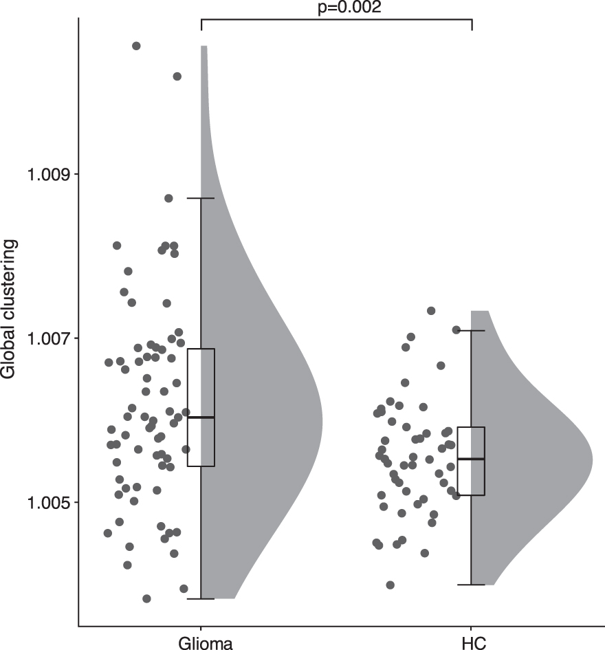
Global clustering in HCs and glioma patients. Patients had higher global clustering compared with HCs (U = 5040, p = 0.002).

Table 2.

Median and Interquartile Range Values of All Group Comparisons

	PLI	AECc
	Median (IQR)	Median (IQR)
Patients
Global clustering (a)	1.0060 (1.0054 to 1.0069)	1.0013 (1.0011 to 1.0014)
Relative theta power (b)	0.1475 (0.1378 to 0.1636)
Functional connectivity (c)	0.1937 (0.1950 to 0.1971)
Local clustering—tumor (d)	0.1919 (0.1905 to 0.1944)	0.5639 (0.5608 to 0.5694)
Local clustering—non-tumor (d)	0.1918 (0.1901 to 0.1931)	0.5634 (0.5600 to 0.5677)
Local clustering (z-scores)—tumor (e)	0.1427 (−0.2713 to 0.8840)	−0.1830 (−0.8391 to 0.8754)
Local clustering (z-scores)—non-tumor (e)	0.1395 (−0.3753 to 0.5259)	−0.3519 (−1.0030 to 0.4683)
HCs
Global clustering (a)	1.0055 (1.0051 to 1.0059)	1.0010 (1.0009 to 1.0012)
Relative theta power (b)	0.1457 (0.1449 to 0.1464)
Functional connectivity (c)	0.1951 (0.1940 to 0.1962)
High global clustering group
Local clustering—tumor (f)	0.9360 (0.3092 to 1.3766)
Local clustering—non-tumor (g)	1.0612 (0.3084 to 1.3965)
Power—tumor (h)	0.1505 (0.1384 to 0.1683)
Power—non-tumor (i)	0.1479 (0.1380 to 0.1773)
Average connectivity—tumor (j)	0.1961 (0.1947 to 0.1977)
Average connectivity—non-tumor (k)	0.1946 (0.1937 to 0.1966)
Healthy local clustering—tumor (l)	0.1914 (0.1912 to 0.1915)
Normal global clustering group
Local clustering—tumor (f)	0.0119 (−0.2815 to 0.4535)
Local clustering—non-tumor (g)	−0.0053 (−0.4942 to 0.2918)
Power—tumor (h)	0.1509 (0.1344 to 0.1731)
Power—non-tumor (i)	0.1455 (0.1360 to 0.1603)
Average connectivity—tumor (j)	0.1951 (0.1926 to 0.1974)
Average connectivity—non-tumor (k)	0.1948 (0.1938 to 0.1973)
Healthy local clustering—tumor (l)	0.1915 (0.1914 to 0.1917)

(x) corresponds to “Table 2(x)” in the results section.

AECc, corrected amplitude envelope correlation; HCs, healthy controls; IQR, interquartile range; PLI, phase lag index.

Local clustering differences between tumor and non-tumor regions are explained by healthy regional variation

Local clustering in tumor regions (regions containing tumor per patient: mean = 13.409, SD = 6.701) was significantly higher than local clustering in non-tumor regions [PLI: W = 1632, p = 0.043; AECc: W = 1464, p = 0.287; Table 2(d)]. This difference did not relate to tumor size, as local tumor clustering did not relate to absolute tumor volume [Spearman's Rho(71) = 0.001, p = 0.994] or relative tumor volume (Spearman's Rho = −0.005, p = 0.970). However, when taking healthy clustering into account using z-scores, no difference between local clustering in tumor and non-tumor regions remained [PLI: W = 1554, p = 0.114; AECc: W = 1554, p = 0.114; Table 2(e)], indicating that local clustering did not differ between tumor and non-tumor regions beyond the normal healthy regional variation. Moreover, this result could indicate that gliomas are located more often in regions with high local clustering in HCs. Indeed, a post hoc analysis showed a significant positive relationship between glioma occurrence and healthy local clustering [Fig. 3, PLI: r(76) = 0.349, p = 0.002].

FIG. 3.

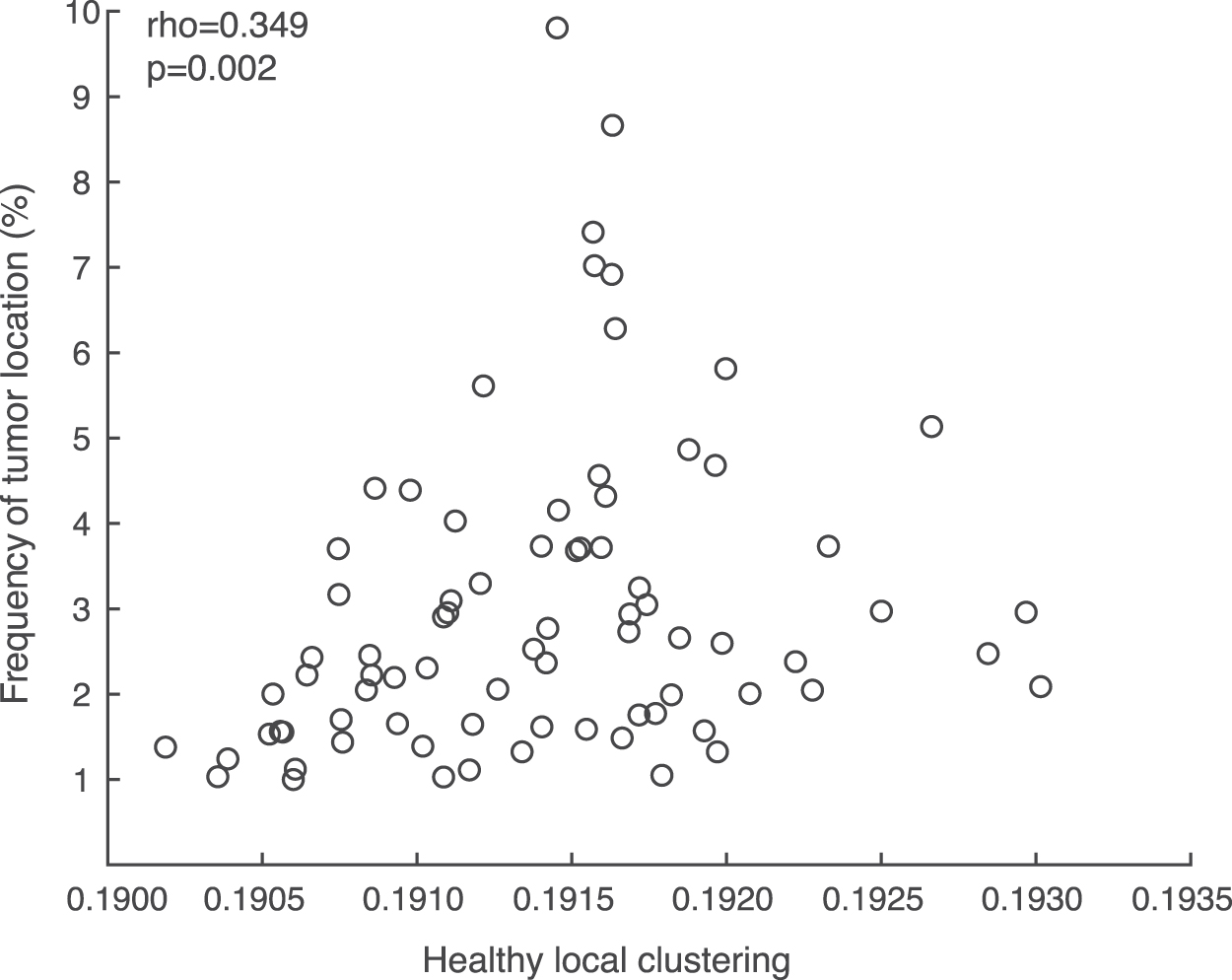
Correlation between average local clustering in the healthy network and overlap with tumors. Gliomas were located more frequently in regions with higher local clustering in the HCs [r(76) = 0.349, p = 0.002].

Local clustering does not relate to distance from the tumor

No association between local clustering and Euclidean distance from the tumor was found (Fig. 4A, PLI: beta = 0.315, 95% confidence interval [CI] [−0.370 to 1.000], p = 0.361, AECc: beta = −0.511, 95% CI [−1.279 to 0.256], p = 0.191).

FIG. 4.

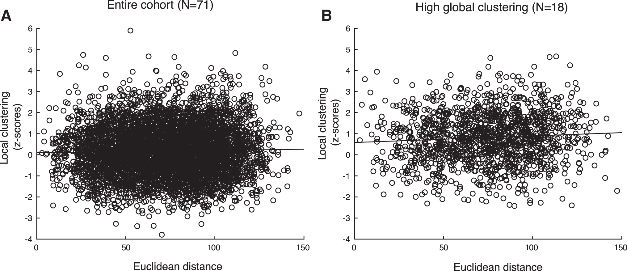
Scatterplot of local clustering and the Euclidean distance between the tumor and all brain regions. (A) Entire cohort. (B) Patients with high global clustering. No association between local clustering and Euclidean distance from the tumor was found for the entire cohort (beta = 0.315, 95% CI [−0.370 to 1.000], p = 0.361) nor for the high clustering group (beta = 0.334, 95% CI [−1.053 to 1.721, p = 0.636]). CI, confidence interval.

Patients with high global clustering have a distinct profile

When analyzing the subgroups of patients with high (n = 18) versus normal (n = 53) global clustering, patients with high global clustering were younger (U = 310, p = 0.027; Table 1). There were no group differences in terms of sex [χ ²(1, n = 71) = 0.143, p = 0.705], KPS [≤80 vs. ≥90, χ ²(1, n = 68) = 0.101, p = 0.751], tumor histology [astrocytoma, oligodendroglioma, or oligoastrocytoma, χ ²(2, n = 71) = 0.352, p = 0.839], tumor grade [grade II vs. grade III/IV, χ ²(1, n = 71) = 0.115, p = 0.735], tumor volume (U = 378, p = 0.191), IDH mutation status [χ ²(1, n = 54) = 0.705, p = 0.401], and presence of epilepsy [χ ²(1, n = 71) = 0.288, p = 0.592; Table 1].

Further, higher local tumor clustering [PLI: U = 1667, p = 0.001; Table 2(f)] as well as local non-tumor clustering [PLI: U = 1599, p < 0.001; Table 2(g)] was found in the patients with high global clustering compared with the rest of the cohort, taking healthy regional variance into account by using z-scores (Fig. 5).

FIG. 5.

Tumor and non-tumor local clustering expressed as z-scores (based on the HC cohort) for patients with highest global clustering (top 25%) and the rest of the glioma patients. Patients with high global clustering had higher tumor (U = 1667, p = 0.001) and non-tumor (U = 1599, p < 0.001) clustering compared with the rest of the cohort.

Within the high global clustering group, no association between local clustering and Euclidean distance from the tumor was found (Fig. 4B, PLI: beta = 0.334, 95% CI [−1.053 to 1.721], p = 0.636, AECc: beta = 0.152, 95% CI [−1.174 to 1.479], p = 0.822). The high global clustering group did not differ from the rest of the cohort in terms of relative power [tumor: U = 656, p = 0.921, Table 2(h); non-tumor: U = 704, p = 0.463, Table 2(i)] or functional connectivity [PLI tumor: U = 755, p = 0.159, Table 2(j); PLI non-tumor: U = 582, p = 0.387; Table 2(k)]. Also, there was no difference in healthy local clustering of tumor locations between patients from the high and normal global clustering groups, although tumors in patients from the high global clustering group tended to occur more often in less locally clustered regions in the healthy brain network [PLI: U = 504, p = 0.058, Fig. 6, Table 2(l)].

FIG. 6.

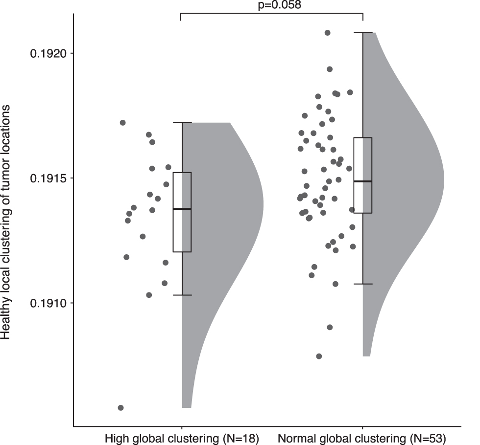
Healthy local clustering at the tumor locations of patients with high global clustering and the rest of the cohort. Tumors of patients with high global clustering tended to locate in regions that have lower clustering in HCs as compared with tumors of patients with normal global clustering (U = 504, p = 0.058).

Discussion

In this large cohort of glioma patients, higher theta band global clustering was observed compared with HCs, replicating previous research (Bosma et al., 2009; van Dellen et al., 2012). Locally, tumor regions did not show higher local clustering than non-tumor regions when taking normal regional variation in clustering into account. Further, no association between local clustering and distance from the tumor was found. Interestingly, post hoc analysis suggests that gliomas are generally located more often in brain regions characterized by higher clustering in the healthy brain network. In contrast, it seemed that the tumor location of patients with pathologically increased global clustering (top 25%) predominantly occurred in regions that were less clustered in the healthy brain network. These patients were also younger than those with normal global clustering.

No evidence was found for the hypotheses that the increase in global clustering in glioma patients is due to increased local clustering of the tumor region or a distance-dependent increase in clustering that decays further from the tumor. Instead, we report widespread increases in local clustering in a subset of patients with high global clustering, suggesting that the entire functional brain network is diffusely altered in these patients. Propagation of functional alterations through the network could be due to cascading network failure caused by local brain lesions, eventually leading to global network dysfunction (Stam, 2014). Although signs of such propagation were not observed due to the cross-sectional nature of the patient cohort, it is still plausible that increases in clustering start locally and eventually affect the whole network in glioma patients. Particularly in low-grade glioma, connectivity changes may have been ongoing for a longer period, since these tumors may be present years before the onset of symptoms and subsequent diagnosis.

Explorative post hoc results showed that gliomas occur more often in regions that have higher local clustering in the healthy functional brain network. The link between the location of focal pathology and local network characteristics has also been established in other neurological diseases. In Alzheimer's disease, amyloid-beta deposition is highest in cortical hubs in the healthy brain network, that is, regions that play a central role in the network (Buckner et al., 2009). Moreover, a meta-analysis of different brain disorders characterized by lesions concluded that lesions were more likely to be located in regions that are marked as hubs in healthy subjects (Crossley et al., 2014). Our results support the idea that regional preferences of pathology may relate to local network topology. The pathophysiology underlying these findings in glioma remains unknown, warranting future studies to look at cellular and metabolic processes in these regions in more detail.

Interestingly, it seemed that tumors in patients with high global clustering were more often located in regions with lower clustering in the healthy brain network. Since this finding contrasts the group-level positive relationship between tumor occurrence and healthy local clustering, it may thus indicate that tumors that occur in normally less clustered regions disrupt global network functioning more than tumors that occur in normally more clustered regions. Or inversely, when the damaged region is part of a local cluster of highly interconnected nodes, these regions may be able to provide protection against global propagation of damage. This idea is supported by a modeling study in which typical brain activity of patients with gliomas was simulated: Gliomas in regions with low local clustering resulted in larger disruption of global functional connectivity, compared with lesions occurring in highly clustered regions (van Dellen et al., 2013). Perhaps regions with high clustering are able to “buffer” more than low clustered regions, thereby reducing the effect of damage. Future (modeling) studies should address how the interplay between premorbid local clustering and a growing tumor impacts global network alterations.

Patients in the high global clustering group were significantly younger than patients with normal global clustering. In general, younger brains are believed to encompass more plasticity (Lu et al., 2004), which could indicate that these brains might be more prone to network changes when pathology occurs. However, these network alterations may not be beneficial in this patient population, since higher global clustering has been associated with poorer cognitive performance in glioma patients (van Dellen et al., 2012). Moreover, despite the lack of differences in tumor type or grade between our subgroups, younger patients generally have lower grade gliomas and more often have IDH-mutated gliomas than older patients. We, therefore, cannot disentangle the true effects of age versus glioma subtype, particularly as different glioma subtypes also tend to occur in spatially distinct regions (Darlix et al., 2017). The current results spark the question as to whether there is a complex interplay between tumor localization and subtype, the premorbid functional brain network, and the subsequent functional network alterations that relate to cognitive decline and epilepsy.

A limitation of this study is that pathological brain tissue, for example, brain tumors, may influence the MEG signal. An increase in MEG power around brain tumors is usually observed in the delta frequency band (de Jongh et al., 2003), which was, therefore, not investigated in this study. Nonetheless, we concluded that our results were not due to power differences after investigating the relationship between global clustering and theta power, as well as differences in theta power between the subgroups.

Conclusions

Brain networks of a subset of glioma patients are disturbed on a global level: No location- or distance-dependence of altered clustering could be determined in these patients. Gliomas tend to occur in regions that have high clustering in healthy brain networks. Nonetheless, it also seems that gliomas located in regions with low healthy clustering have a more detrimental effect on the whole-brain network.

Footnotes

Acknowledgments

The authors would like to thank Nico Akemann, Ndedi Sijsma, Karin Plugge, Marieke Alting Siberg, Marlous van den Hoek, and Peter-Jan Ris for the MEG acquisitions.

Authors' Contributions

J.D., S.D.K., A.H., and L.D. had a major role in the acquisition of the data. J.D., S.D.K., T.N., and L.D. designed and conceptualized the study. J.D., S.D.K., and L.D. did the analysis of the data. J.D., S.D.K., T.N., and L.D. did the interpretation of the data. J.D. and S.D.K. drafted the article for intellectual and technical content. All other authors (T.N., P.C.d.W.H., D.P.N., M.K., J.J.G.G., J.C.R., C.J.S., M.M.S., A.H., and L.D.) also took part in writing, reviewing, and revising the article.

Author Disclosure Statement

J.J.G.G. receives research fees from Biogen, Genzyme, Novartis, and MerckSerono and is President of the Netherlands Institute for Health Research and Development. All other authors have no competing financial interests to report.

Funding Information

This study was funded by the Dutch Epilepsy Foundation (NEF 08-08, 09-09), the Dutch MS research foundation (02-358b, 05-358c, 08-650, 09-358d, 10-718), the Nederlandse Organisatie voor Wetenschappelijk Onderzoek (Veni 016.146.086), and Society in Science (Branco Weiss Fellowship).

References

Aerts

, Fias

, Caeyenberghs

, et al. 2016. Brain networks under attack: robustness properties and the impact of lesions. Brain, 139:3063–3083.

Belgers

, Numan

, Kulik

, et al. 2020. Postoperative oscillatory brain activity as an add-on prognostic marker in diffuse glioma. J Neurooncol, 147:49–58.

Bosma

, Reijneveld

, Klein

, et al. 2009. Disturbed functional brain networks and neurocognitive function in low-grade glioma patients: a graph theoretical analysis of resting-state MEG. Nonlinear Biomed Phys, 3:9.

Brookes

, Hale

, Zumer

, et al. 2011. Measuring functional connectivity using MEG: methodology and comparison with fcMRI. Neuroimage, 56:1082–1104.

Buckner

, Sepulcre

, Talukdar

, et al. 2009. Cortical hubs revealed by intrinsic functional connectivity: mapping, assessment of stability, and relation to Alzheimer's disease. J Neurosci, 29:1860–1873.

Carbo

EWS

, Hillebrand

, van Dellen

, et al. 2017. Dynamic hub load predicts cognitive decline after resective neurosurgery. Sci Rep, 7:42117.

Crossley

, Mechelli

, Scott

, et al. 2014. The hubs of the human connectome are generally implicated in the anatomy of brain disorders. Brain, 137:2382–2395.

Darlix

, Deverdun

, Menjot de Champfleur

, et al. 2017. IDH mutation and 1p19q codeletion distinguish two radiological patterns of diffuse low-grade gliomas. J Neurooncol, 133:37–45.

de Jongh

, Baayen

, de Munck

, et al. 2003. The influence of brain tumor treatment on pathological delta activity in MEG. Neuroimage, 20:2291–2301.

10.

Derks

, Dirkson

, de Witt Hamer

, et al. 2017. Connectomic profile and clinical phenotype in newly diagnosed glioma patients. NeuroImage Clin, 14:87–96.

11.

Derks

, Kulik

, Wesseling

, et al. 2019. Understanding cognitive functioning in glioma patients: the relevance of IDH-mutation status and functional connectivity. Brain Behav, 9:e01204.

12.

Derks

, Reijneveld

, Douw

. 2014. Neural network alterations underlie cognitive deficits in brain tumor patients. Curr Opin Oncol, 26:627–633.

13.

Derks

, Wesseling

, Carbo

EWS

, et al. 2018. Oscillatory brain activity associates with neuroligin-3 expression and predicts progression free survival in patients with diffuse glioma. J Neurooncol, 140:403–412.

14.

Fox

, King

. 2018. Functional connectivity in adult brain tumor patients: a systematic review. Brain Connect, 8:381–397.

15.

Hillebrand

, Barnes

, Bosboom

, et al. 2012. Frequency-dependent functional connectivity within resting-state networks: an atlas-based MEG beamformer solution. Neuroimage, 59:3909–3921.

16.

Hillebrand

, Tewarie

, van Dellen

, et al. 2016. Direction of information flow in large-scale resting-state networks is frequency-dependent. Proc Natl Acad Sci U S A, 113:3867–3872.

17.

VKY

, Reijneveld

, Enting

, et al. 2014. Changing incidence and improved survival of gliomas. Eur J Cancer, 50:2309–2318.

18.

Jenkinson

, Bannister

, Brady

, et al. 2002. Improved optimization for the robust and accurate linear registration and motion correction of brain images. Neuroimage, 17:825–841.

19.

Karnofsky

, Abelmann

, Craver

, 1948. The use of nitrogen mustards in the palliative treatment of carcinoma. Cancer, 1:634–656.

20.

Lai

, Demuru

, Hillebrand

, et al. 2018. A comparison between scalp- and source-reconstructed EEG networks. Sci Rep, 8:12269.

21.

Louis

, Ohgaki

, Wiestler

, et al. 2007. The 2007 WHO classification of tumours of the central nervous system. Acta Neuropathol, 114:97–109.

22.

, Pan

, Kao

, et al. 2004. Gene regulation and DNA damage in the ageing human brain. Nature, 429:883–891.

23.

Onnela

, Saramäki

, Kertész

, et al. 2005. Intensity and coherence of motifs in weighted complex networks. Phys Rev, E71:065103.

24.

Rubinov

, Sporns

. 2010. Complex network measures of brain connectivity: uses and interpretations. Neuroimage, 52:1059–1069.

25.

Stam

. 2014. Modern network science of neurological disorders. Nat Rev Neurosci, 15:683–695.

26.

Stam

, Nolte

, Daffertshofer

. 2007. Phase lag index: assessment of functional connectivity from multi channel EEG and MEG with diminished bias from common sources. Hum Brain Mapp, 28:1178–1193.

27.

Taulu

, Hari

. 2009. Removal of magnetoencephalographic artifacts with temporal signal-space separation: demonstration with single-trial auditory-evoked responses. Hum Brain Mapp, 30:1524–1534.

28.

Taulu

, Simola

. 2006. Spatiotemporal signal space separation method for rejecting nearby interference in MEG measurements. Phys Med Biol, 51:1759–1768.

29.

Tewarie

, Hillebrand

, van Dellen

, et al. 2014a. Structural degree predicts functional network connectivity: a multimodal resting-state fMRI and MEG study. Neuroimage, 97:296–307.

30.

Tewarie

, Schoonheim

, Schouten

, et al. 2015. Functional brain networks: linking thalamic atrophy to clinical disability in multiple sclerosis, a multimodal fMRI and MEG Study. Hum Brain Mapp, 36:603–618.

31.

Tewarie

, Steenwijk

, Tijms

, et al. 2014b. Disruption of structural and functional networks in long-standing multiple sclerosis. Hum Brain Mapp, 35:5946–5961.

32.

Tzourio-Mazoyer

, Landeau

, Papathanassiou

, et al. 2002. Automated anatomical labeling of activations in SPM using a macroscopic anatomical parcellation of the MNI MRI single-subject brain. Neuroimage, 15:273–289.

33.

van Dellen

, Douw

, Hillebrand

, et al. 2012. MEG network differences between low- and high-grade glioma related to epilepsy and cognition. PLoS One, 7:e50122.

34.

van Dellen

, Douw

, Hillebrand

, et al. 2014. Epilepsy surgery outcome and functional network alterations in longitudinal MEG: a minimum spanning tree analysis. Neuroimage, 86:354–363.

35.

van Dellen

, Hillebrand

, Douw

, et al. 2013. Local polymorphic delta activity in cortical lesions causes global decreases in functional connectivity. Neuroimage, 83:524–532.

36.

van Klink

, van Rosmalen

, Nenonen

, et al. 2017. Automatic detection and visualisation of MEG ripple oscillations in epilepsy. NeuroImage Clin, 15:689–701.

37.

Wang

, Meng

. 2016. Functional brain network alterations in epilepsy: a magnetoencephalography study. Epilepsy Res, 126:62–69.

38.

Wang

, Douw

, Hernández

, et al. 2010. Effect of tumor resection on the characteristics of functional brain networks. Phys Rev, E82:021924.

39.

Watts

, Strogatz

. 1998. Collective dynamics of “small-world” networks. Nature, 393:440–442.

40.

Whalen

, Maclin

, Fabiani

, et al. 2008. Validation of a method for coregistering scalp recording locations with 3D structural MR images. Hum Brain Mapp, 29:1288–1301.