
Abstract
Aim:
In this work, we propose the novel use of adaptively constrained independent vector analysis (acIVA) to effectively capture the temporal and spatial properties of dynamic blood-oxygen-level-dependent (BOLD) activity (dBA), and we efficiently quantify the spatial property of dBA (sdBA). We also propose to incorporate dBA into the study of brain dynamics to gain insight into activity-connectivity co-evolution patterns.
Introduction:
Studies of the dynamics of the human brain using functional magnetic resonance imaging (fMRI) have enabled the identification of unique functional network connectivity (FNC) states and provided new insights into mental disorders. There is evidence showing that both BOLD activity, which is captured by fMRI, and FNC are related to mental and cognitive processes. However, a few studies have evaluated the inter-relationships of these two domains of function. Moreover, the identification of subgroups of schizophrenia has gained significant clinical importance due to a need to study the heterogeneity of schizophrenia.
Methods:
We design a simulation study to verify the effectiveness of acIVA and apply acIVA to the dynamic study of resting-state fMRI data collected from individuals with schizophrenia and healthy controls (HCs) to investigate the relationship between dBA and dynamic FNC (dFNC).
Results:
The simulation study demonstrates that acIVA accurately captures the spatial variability and provides an efficient quantification of sdBA. The fMRI analysis yields synchronized sdBA-temporal property of dBA (tdBA) patterns and shows that the dBA and dFNC are significantly correlated in the spatial domain. Using these dynamic features, we identify schizophrenia subgroups with significant differences in terms of their clinical symptoms.
Conclusion:
We find that brain function is abnormally organized in schizophrenia compared with HCs since there are less synchronized sdBA-tdBA patterns in schizophrenia and schizophrenia prefers a component that merges multiple brain regions. Identification of schizophrenia subgroups using dynamic features inspires the use of neuroimaging in studying the heterogeneity of disorders.
Impact statement
This work introduces the use of joint blind source separation for the study of brain dynamics to enable efficient quantification of the spatial property of dynamic blood-oxygen-level-dependent (BOLD) activity to provide insight into the relationship of dynamic BOLD activity and dynamic functional network connectivity. The identification of subgroups of schizophrenia using dynamic features allows the study of heterogeneity of schizophrenia, emphasizing the importance of functional magnetic resonance imaging analysis in the study of brain activity and functional connectivity to gain a better understanding of the human brain, especially the brain with a mental disorder.
Introduction
Studies of the dynamics of human brain function using neuroimaging data have achieved great success in identifying unique biomedical patterns that enable a better understanding of the functional differences between the healthy and disordered brain (Assaf et al., 2010; Etkin et al., 2009; Hutchison et al., 2013; Lefebvre et al., 2016; Rashid et al., 2014; Uddin et al., 2011).
Functional magnetic resonance imaging (fMRI) is one of the most commonly used imaging modalities and measures the blood-oxygen-level-dependent (BOLD) activity in human brain during either resting- or task-evoked state (Allen et al., 2014; Kucyi and Davis, 2014; Sakoğlu et al., 2010; Verley et al., 2018; Wang et al., 2010). Most dynamic studies obtain a functional connectivity (FC) or functional network connectivity (FNC) matrix, which measures the association between the BOLD activity of different functional regions or coherent networks, as a function of time. A dynamic FNC (dFNC) analysis allows a systematical study of evolving functional patterns by jointly taking multiple brain networks into consideration (Calhoun et al., 2014; Mennigen et al., 2019).
There is rich work showing that both BOLD activity and F(N)C are related to mental and cognitive processes (Britz et al., 2009; Hutchison and Morton, 2016; Marusak et al., 2017; McIntosh et al., 2008; Pereira et al., 2019). Differences in BOLD activity and FNC have been separately reported in multiple mental disorders, especially in schizophrenia, such as reduced amplitude of low-frequency fluctuation (ALFF) in cuneus (Hoptman et al., 2010; Turner et al., 2013), reduced BOLD activation in anterior cingulate gyrus (Baiano et al., 2007; Schultz et al., 2012), dysconnectivity in default mode network (DMN; Mingoia et al., 2012; Van Den Heuvel and Pol, 2010), and dysconnectivity between thalamus and sensory regions (Calhoun et al., 2009; Guller et al., 2012; Kühn and Gallinat, 2013; Malaspina et al., 2004; Zhou et al., 2007). However, the association between time-varying, that is, dynamic BOLD activity (dBA) and dFNC is not well studied and it is desirable to incorporate dBA to gain insight into the activity-connectivity co-evolution by identifying highly correlated patterns between dBA and dFNC.
In Fu et al. (2018), the authors investigate the associations between dBA and dFNC in temporal domain, that is, they measure dBA and dFNC by using the temporal variabilities of functional networks and observe that dBA and dFNC are significantly correlated in time in some cases and patients with schizophrenia show lower or nonexistent associations between dBA and dFNC compared with the healthy controls (HCs). However, similar to Fu et al. (2018), most previous studies conduct a dFNC analysis by using the time courses of BOLD activity by assuming the spatial domain is static (Jafri et al., 2008; Calhoun et al., 2014; Allen et al., 2014; Weber et al., 2020).
Spatial variation of BOLD activity is observed as a change in the volume of a functional network or variations in the activated regions within a functional network and has started to attract attention, since they enrich the dynamic study of brain function (Iraji et al., 2019a,b, 2020). Previous studies have shown that simultaneously considering temporal and spatial changes yields more distinguishable resting-state networks (RSNs) between subject groups (Jie et al., 2018; Kottaram et al., 2018; Iraji et al., 2020). Studies that compute dFNC by using the spatial maps of brain networks have also emphasized the importance of the assumption of spatial variability in a dynamic study, by detecting significant differences between the patients with mental disorder such as between those with schizophrenia and the HCs (Bhinge et al., 2019a,b; Ma et al., 2014).
However, the spatial activation patterns of dBA themselves are not well explored primarily due to the lack of effective quantification strategies of spatial property of dBA (sdBA). An efficient quantification of sdBA does not only enable the investigation of the spatial activation patterns of dBA but also leads to a study of activity-connectivity co-evolution using sdBA and dFNC that is computed by using the spatial maps (sdFNC) of functional networks.
The extraction and efficient quantification of the dynamic features captured through temporal and spatial variation leads one to analyze their importance in studying a mental disorder such as schizophrenia. There has been significant interest in studying the subtypes of schizophrenia (Dwyer et al., 2018; Geisler et al., 2015; Jablensky, 2006, 2010) to gain a better understanding of the uncertainty in whether a precision medicine is needed (Senn, 2018) during clinical diagnosis and treatment. Subtypes of schizophrenia have been studied by using genetic information (Hallmayer et al., 2005; Morar et al., 2018; Sayın et al., 2013) but not yet using neuroimaging modalities such as fMRI data that have been successfully used in the study of schizophrenia (Calhoun and Adalı, 2009; Geisler et al., 2015; Ma et al., 2012).
Our previous work showed that fMRI alone can identify subgroups of schizophrenia that demonstrated significant differences in terms of clinical symptoms and it helps understand the heterogeneity of schizophrenia (Long et al., 2020). However, these subgroups were identified through static imaging features. This motivates an investigation of the effectiveness of dynamic neuroimaging features for identifying and studying the heterogeneity of mental disorders such as schizophrenia.
Both temporal and spatial variabilities of BOLD activity are important to gain a better understanding of brain dynamics. However, existing methods such as group independent component analysis (ICA; Calhoun et al., 2001) and joint ICA (Calhoun et al., 2006) can only effectively capture either temporal variability or spatial variability by making relatively strong assumptions. In this work, we propose the novel use of a recent method, adaptively constrained independent vector analysis (acIVA; Bhinge et al., 2019b), that enables us to simultaneously capture the dFNC and dBA in the spatial and temporal domain, and acIVA also provides an effective quantification of sdBA, as part of the algorithm.
AcIVA is able to precisely preserve spatial variability by adaptively tuning the constraint parameter that controls the spatial association between reference signals and the source estimates. More importantly, measuring the association between reference signals and the source estimates as part of the acIVA algorithm provides an efficient quantification of sdBA. The acIVA method also reduces the undesirable effects of high dimensionality that frequently arise during a dynamic study. We describe the issue of high dimensionality and its relation to the dynamic study in the Data Formation for Dynamic Analysis section. In addition, acIVA eliminates the tough alignment process across multiple decompositions due to the use of reference signals (Bhinge et al., 2019b).
To study the novel use of acIVA to capture the dynamic features, we propose a simulation study and demonstrate that acIVA yields a desirable performance in capturing spatial dynamics by accurately recovering the association between reference signals and the targeted estimates. The adaptively tuned constraint parameter ρ provides the closest lower bound for the association, hence preserving the spatial variation patterns across datasets.
We apply acIVA to extract dynamic features from a resting-state fMRI dataset acquired from 179 subjects (88 schizophrenia subjects and 91 HCs). We quantify the temporal property of dBA (tdBA) by using fractional ALFFs (fALFFs) of network time courses to conduct a comparison between tdBA and sdBA. To study the activity-connectivity co-evolution of dBA and dFNC, dFNC is measured by using the dependence among spatial maps and the correlation between sdBA and sdFNC is computed.
The analysis results show that tdBA and sdBA pairs of the same functional network have higher correlation than those of different networks, and sdBA yields higher correlation with the network connectivity that is associated with the same network. However, schizophrenia subjects show fewer significantly correlated sdBA and tdBA pairs and favor a complex component that merges multiple brain regions—super parietal, visual, and cerebellum (SP-V-C)—when compared with HCs, suggesting that the brain function is abnormally organized in schizophrenia; hence, more brain regions are simultaneously activated for a certain intrinsic function. Most importantly, we identify subgroups of schizophrenia by using the tdBA-sdBA association and the sdBA-sdFNC co-evolution, and we detect significant differences across subgroups in terms of their clinical symptoms that are measured by the positive and negative syndrome scale (PANSS) scores (Kay et al., 1987). This observation inspires further study of the heterogeneity of mental disorders by using neuroimaging modalities such as fMRI.
The rest of the article is organized as follows. The Materials and Methods section presents the framework of using acIVA for dynamic analysis of fMRI data, including data formation by adopting the sliding window approach, a detailed introduction of acIVA algorithm, the extraction of reference signal, and the quantification of dBA and dFNC. The Results section shows the simulation results and the application to real fMRI data. Finally, we conclude in the Discussion section and point out the limitations of this work and possible interesting future directions.
Materials and Methods
Institutional Review Board approval statement
Institutional Review Board approval was obtained for the study. All participants provided informed consent. This work is not a clinical trial.
Data acquisition and preprocessing
We used resting-state fMRI data from the Center of Biomedical Research Excellence (COBRE) that is available on the collaborative informatics and neuroimaging suite data exchange repository (Scott et al., 2011; Çetin et al., 2014; Aine et al., 2017). The data include 88 schizophrenia subjects (average age:
For this study, the participants were asked to keep their eyes open during the entire scanning period. All images were collected on a single 3-Tesla Siemens Trio scanner with a 12-channel radio frequency coil by using the following parameters: echo time = 29 msec, repetition time = 2 sec, flip angle = 75°, slice thickness = 3.5 mm, slice gap = 1.05 mm, and voxel size
Data formation for dynamic analysis
The sliding window approach facilitates the dynamic study of fMRI data that are acquired within a certain duration (Ma et al., 2014). In a sliding window approach, the entire scanning period is divided into overlapping windows of length Tw
, yielding L windows for each subject, as shown in Figure 1. In our case, this results in
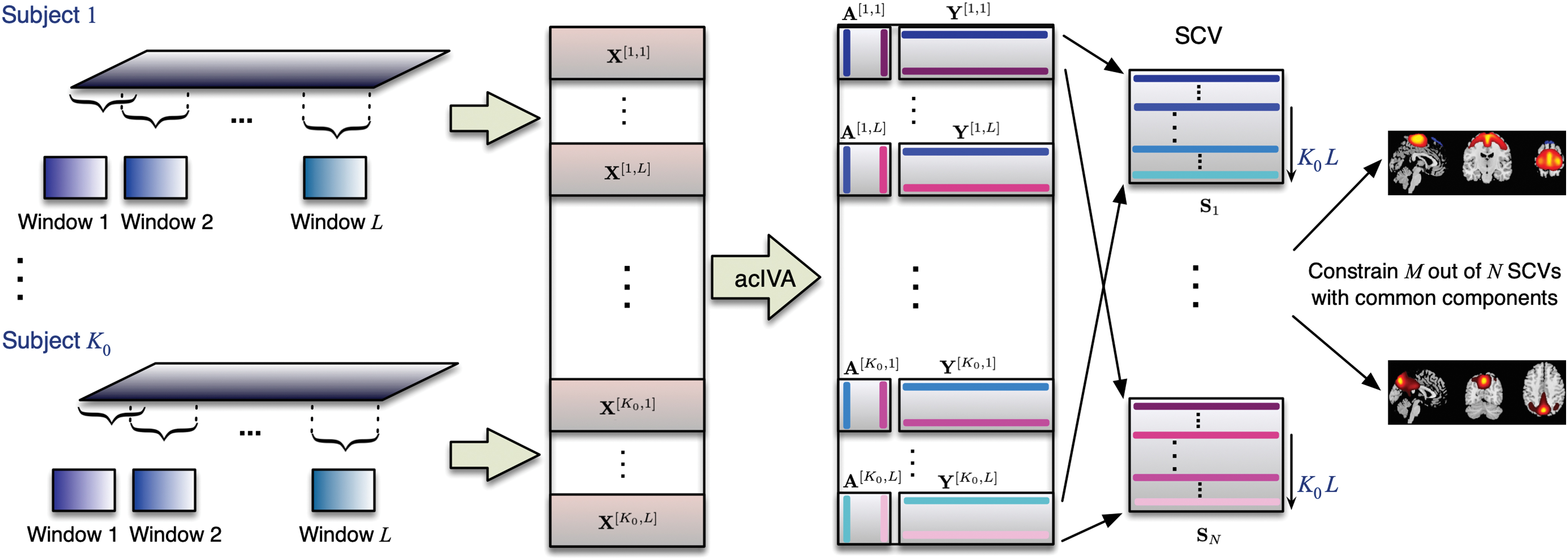
Dynamic study using acIVA with the sliding window approach on a subset of K 0 subjects. Applying acIVA to the windowed datasets with the spatial maps of common components as reference signals yields the time courses and spatial maps for each dataset. The constrained SCVs contain corresponding components from different windows and subjects. acIVA, adaptively constrained independent vector analysis; SCV, source component vector. Color images are available online.
Independent vector analysis (IVA) is a data-driven technique that extends ICA to multiple datasets and makes effective use of the dependence across datasets (Adalı et al., 2014). The IVA also relaxes the assumptions made in other joint blind source separation solutions such as group ICA (Calhoun et al., 2001), which assumes a common spatial signal space, and joint ICA (Calhoun et al., 2006), which assumes a common temporal signal space. The IVA simultaneously estimates the demixing matrices of all datasets to obtain dataset-specific time courses and spatial maps, effectively capturing both the temporal and spatial variability of functional networks across datasets (Bhinge et al., 2019a,b; Laney et al., 2014; Ma et al., 2014). However, this flexibility comes at a cost that, with a limited number of samples, the performance of IVA degrades as the number of datasets and/or the model order—the number of sources—increases (Bhinge et al., 2019b; Long et al., 2020). This issue is referred to as a curse of high dimensionality in IVA and is addressed by using a novel algorithm, acIVA, that incorporates reference information into the IVA decomposition.
Adaptively constrained IVA
The acIVA algorithm is a semi-blind source separation technique that incorporates reference information regarding the time courses or spatial maps into the IVA decomposition. This reference information guides the decomposition toward a desirable solution in high-dimensional scenarios, thereby addressing the issue of high dimensionality (Bhinge et al., 2019b). In this section, we introduce the general IVA model followed by a description of the acIVA technique.
Given K datasets each containing V samples, IVA assumes that each dataset is a linear mixture of N independent sources,
where

such that the estimated sources of each dataset are obtained as  denotes the demixing matrices,
The acIVA algorithm guides the decomposition with prior information such as properly selected reference signals for the source components. The IVA decomposition is, hence, achieved by minimizing the cost function in Equation (2) subject to an inequality constraint

where  is the IVA cost function as defined in Equation (2),
Through an adaptive parameter-tuning process, acIVA yields different values of the lower bound
The use of reference signals also effectively reduces the effect of high dimensionality, providing a more robust estimation. In addition, it eliminates the alignment problem across multiple decompositions. In application to the dynamic study of resting-state COBRE fMRI data, this makes it possible to divide the 179 subjects into multiple subsets of K
0 subjects (yielding
Reference signal extraction
In our implementation of acIVA for extracting and quantifying sdBA from multi-subject resting-state fMRI data, we use the spatial maps of exemplar RSN components as reference signals. Possible choices for the exemplar RSNs include the pre-defined RSN templates (Allen et al., 2011) or the group-level RSN components extracted from the same dataset by using group decomposition algorithms such as group ICA (Bhinge et al., 2019a).
In this work, we apply acIVA to the resting COBRE data collected from a schizophrenia group and an HC group, seeking to gain a better understanding of schizophrenia through a fair comparative study of dynamic features, that is, the association between sdBA and tdBA and the co-evolution of sdBA and sdFNC, between groups. Therefore, instead of using arbitrarily pre-defined or estimated RSNs, it is desirable to use common static RSNs that are shared across the subjects of two groups as the reference signals. We extract common RSNs from the data of all 179 subjects by using a common subspace analysis method (Long et al., 2020) and use their spatial maps as reference signals. All the spatial maps are normalized to have zero mean and unit variance.
Analysis of dBA and dFNC
Spontaneous slow fluctuations of correlated activity are a fundamental feature of the resting brain and can be captured as the BOLD signal that reflects neural synchrony between brain regions (Bluhm et al., 2007; van de Ven et al., 2004). A related measure is fALFF that quantifies the amplitude of these low-frequency oscillations. Therefore, we measure tdBA by computing the fALFF of time courses as the fraction of the square root of power spectrum integrated in a low-frequency band (0.025–0.15 Hz) that summarizes the most dominant frequencies of BOLD signal during resting state (Zang et al., 2007; Zou et al., 2008).
Before computing fALFF, the time courses were detrended, motion parameters were regressed (including their derivatives, their squares, and derivatives of their squares), and finally despiked, which involved detecting spikes as determined by the 3dDespike algorithm that is originally included in the Analysis of Functional NeuroImages toolbox (
The fALFF feature of each component is a vector of length L with each entry as the fALFF value of the associated time course in a single window. In this study, there are M RSN components involved, hence yielding M fALFF features. Since the variabilities of the spatial maps of RSNs reflect sdBA, we quantify sdBA by using correlation between the spatial maps of the estimates and the reference signals,
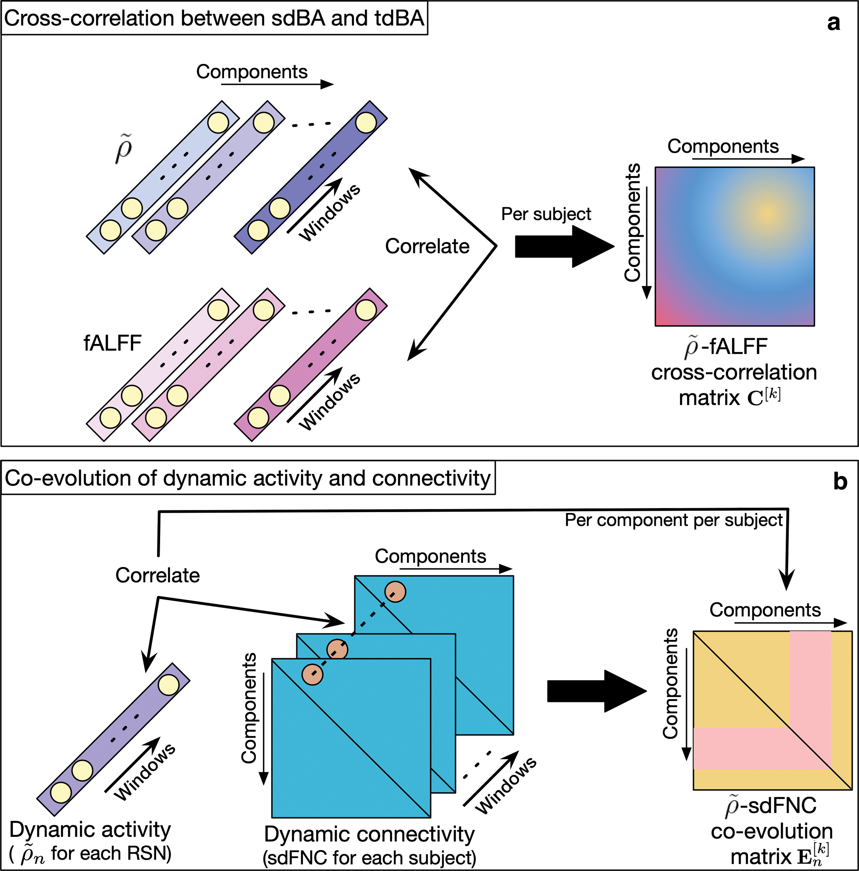
Cross-correlation between sdBA (
As there is evidence that both BOLD activity and network connectivity are related to mental and cognitive processes in the brain, it is desirable to study the co-evolution of BOLD activity and network connectivity. In Fu et al. (2018), the authors studied activity-connectivity co-evolution by using temporal characteristics of the BOLD signal. In this work, we make use of an effective metric
The matrices
Study of schizophrenia heterogeneity
We study the heterogeneity of schizophrenia by identifying subgroups of schizophrenia subjects using k-means clustering to cluster the
After identifying subgroups of schizophrenia, we perform a multivariate analysis of variance (MANOVA) on
Simulation study
In the application of acIVA to real fMRI data, we use the spatial maps of RSNs as reference signals to emphasize the importance of spatial variabilities. Therefore, we first use a simulation study to demonstrate that acIVA is able to accurately recover the spatial variabilities due to the adaptive parameter-tuning process.
The acIVA implementation enables the quantification of sdBA by adaptively tuning the amount of correspondence between the estimated functional networks and the reference signals. We use simulated data to demonstrate the ability of acIVA to accurately capture the underlying spatial variability of dBA. To simulate fMRI-like sources that are super-Gaussian distributed, we generate

Visualization of the correlation matrices and the decomposition results of acIVA in the four cases of simulation. A total of 100 independent realizations are generated for each case. In the ticklabels of x-axis in the boxplots, “H” refers to the results of components that are highly correlated (c
1) with the reference signal, “L” refers to the results of components that are not highly correlated (c
2), and “diff” refers to the cases where we summarize the differences between the tuned values of
Out of the 10 SCVs, we constrain 6 SCVs, where the first component in each of the first 6 SCVs is used as the reference signal, and the other 15 components are used to generate 
The details of four cases where the SCVs are generated to have different correlation matrices are as follows, and the visualization of correlation matrices is illustrated in Figure 3. If the components within an SCV are highly correlated with the reference signal, it means the spatial activation of the component is relatively stationary and does not vary much across datasets. If the components are barely correlated with the reference signal, it means the component varies a lot across datasets in terms of its spatial activation.
Case 1: SCVs 1–3 are generated to have a uniform correlation structure with correlation value
Case 2: SCVs are generated by using the same parameters as in Case 1, except that the low correlation values in SCVs 4–6 are randomly selected from a uniform distribution 

Case 3: SCVs 1–3 are generated to have correlation values
Case 4: SCVs 1 and 2 are generated to have correlation values
We quantify sdBA by using correlation between the spatial maps of the estimates and the reference signals. This metric is reflected in the tuned value of
Results
We summarize the experimental results of both the simulation study and the application to real fMRI data in this section. With the simulation study, we demonstrated that acIVA accurately preserves the spatial variabilities across datasets. When applied to real fMRI data, we investigated the association between the tdBA and sdBA and study the activity-connectivity co-evolution by using spatial variabilities.
Simulation results
We had 100 independent realizations for each of the four cases introduced in the Simulation study section and summarized the results in Figure 3. We used the box plot for comparing values of the tuned
Application to fMRI data
We obtained
Using the common subspace extraction method, we obtained eight components that were shared across all 179 subjects. The spatial maps of
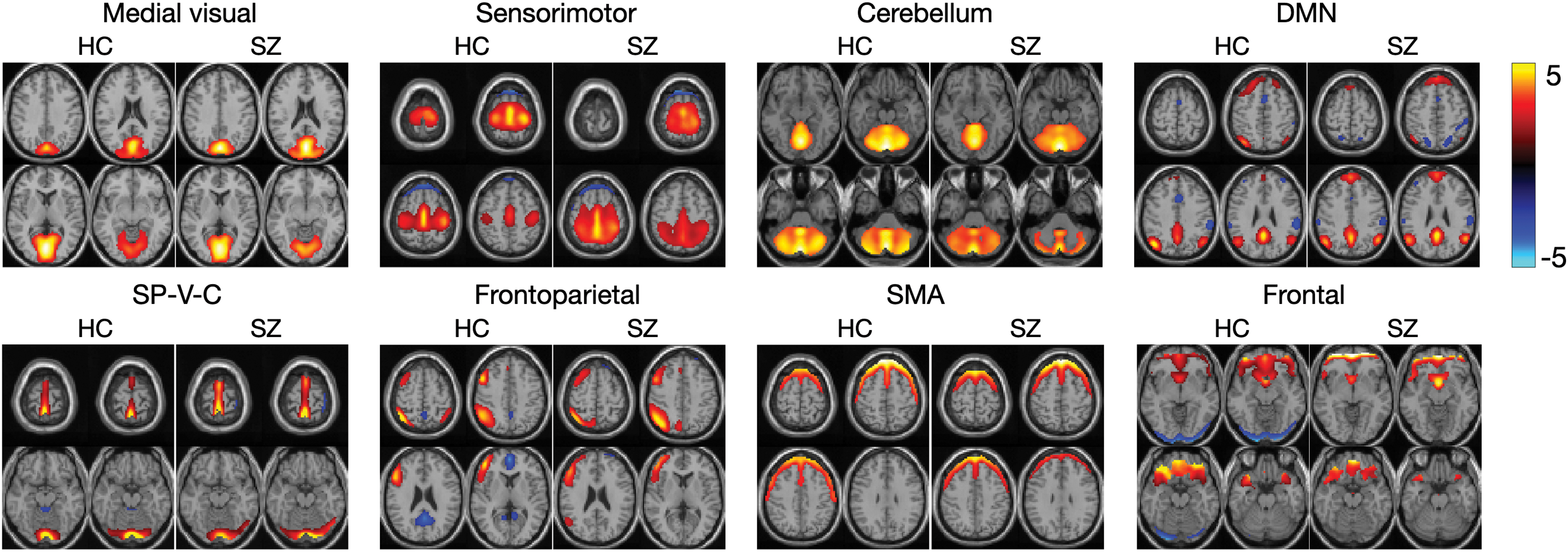
Spatial maps of the eight common RSN components extracted by using IVA-CS for HC and SZ groups. DMN, default mode network; HC, healthy control; IVA-CS, IVA for common subspace analysis; SMA, supplementary motor area; SP-V-C, super parietal, visual, and cerebellum; SZ, schizophrenia. Color images are available online.
The tuned values of
We also computed the normalized mutual information between the estimates and reference signals and compared their values with the correlation values
Co-evolution of activity and connectivity
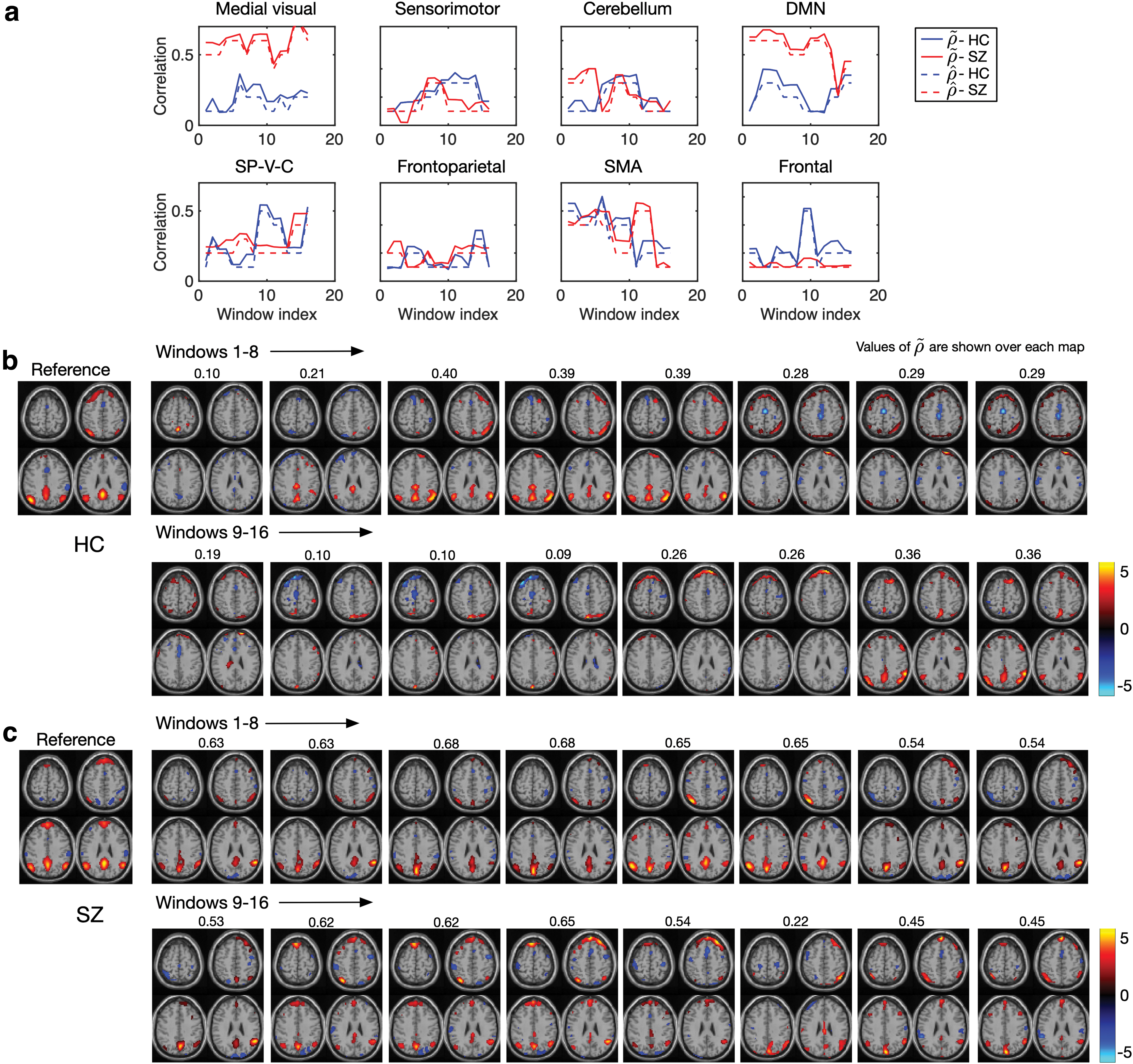
We first investigated the association between sdBA and tdBA (referred to as Case 1 for simplicity in the following context) by computing the cross-correlation between
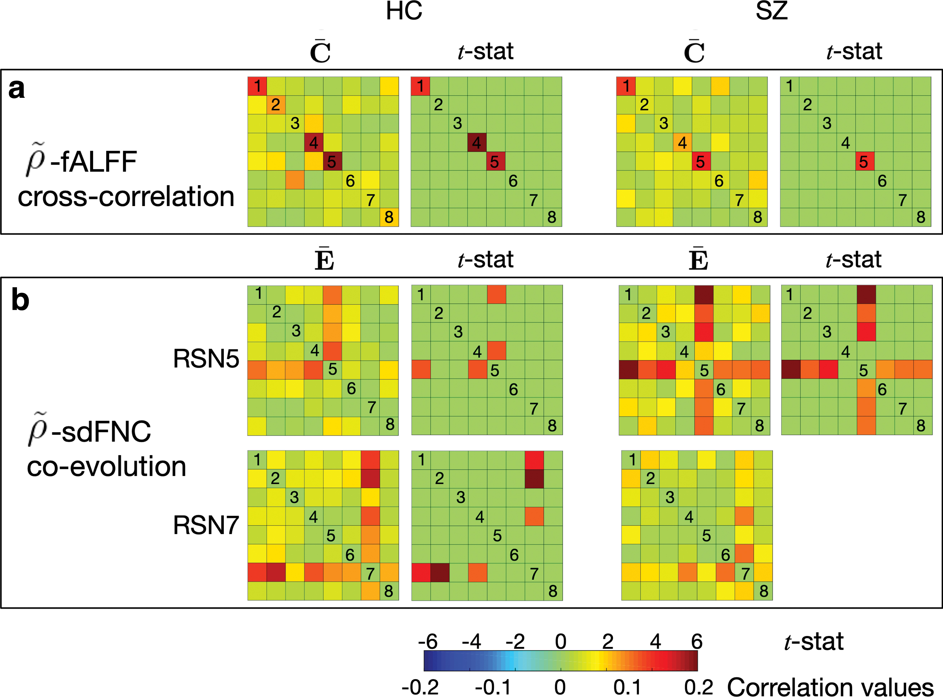
Cross-correlation matrices of two types of dBA
The investigation of the activity-connectivity co-evolution in the spatial domain (referred to as Case 2 for simplicity in the following context) is shown in Figure 6b by demonstrating the mean co-evolution matrices
Identification of subgroups of schizophrenia using dynamic features
We identified subgroups of schizophrenia subjects by clustering
The mean cross-correlation matrices
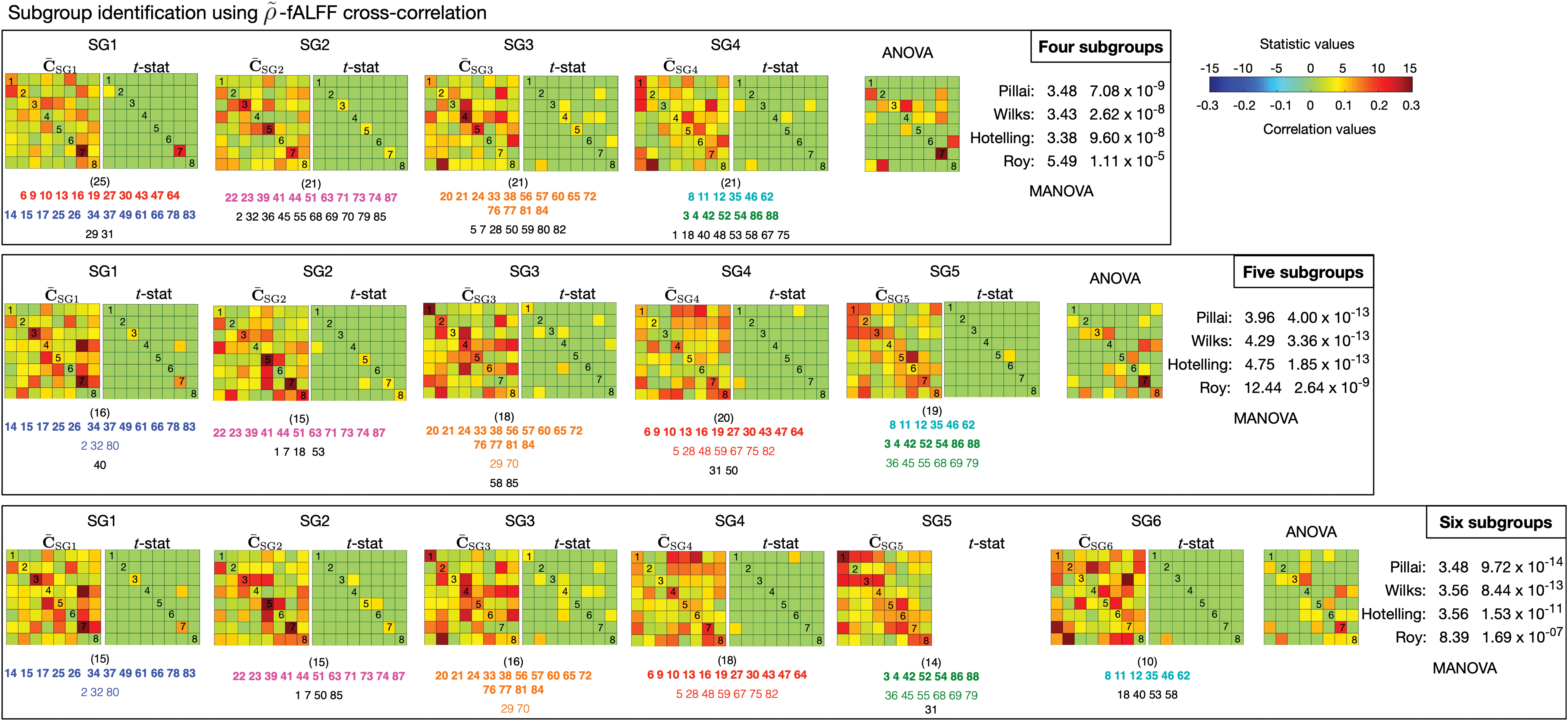
Mean cross-correlation matrices of each subgroup and the statistical test results (with an FDR control) for three scenarios with different values of N s. The consistent subclusters of SZ subjects that are denoted by using numbers k = 1, …, 88 are listed under the correlation matrices using different colors. The colored font in bold refers to subclusters that are consistently detected in all three scenarios, and the regular colored font refers to subclusters that are detected in at least two scenarios. The font in black refers to subjects that do not belong to any consistent subclusters. The numbers in brackets denote the number of subjects in each subgroup. It should be noted that in the fifth subgroup (SG5) in the third scenario, all the correlation values are not significant with FDR control. ANOVA, analysis of variance; MANOVA, multivariate analysis of variance. Color images are available online.
We looked in detail at subjects that were clustered into each subgroup, and we identified some subject clusters that were consistently grouped together, as shown in Figure 7 with numbers denoting subject indices ((
We also compared the clinical symptoms measured by PANSS scores (Kay et al., 1987) across the schizophrenia subgroups that were identified by using neuroimaging data. There is a total of 7 positive, 7 negative, and 16 general PANSS scales that were measured for each subject. To compare the scores across the identified subgroups, we performed a MANOVA on five statistics—mean, standard deviation, median, minimum, and maximum—of all the 30 PANSS across subgroups. The statistics of each PANSS were computed by using the values of all subjects in a single subgroup. Therefore, in this MANOVA, five variables—mean, standard deviation, median, minimum, and maximum—with 30 samples were tested across the
Positive, negative, and general PANSS are three independent categories that can be investigated separately (Kayahan et al., 2005; Peralta and Cuesta, 1994). Therefore, we also investigated the differences across the identified subgroups by looking at the correlation between their positive, negative, and general PANSS for the case when

Correlation between the positive, negative, and general positive and negative syndrome scale scores for each subgroup when N
s = 6 for Case 1
Discussion
In this work, we proposed the use of a semi-blind source separation method acIVA to extract both the spatial and temporal variations across multiple datasets. We first demonstrated that acIVA yielded preferable performance in preserving the spatial variabilities across multiple datasets when using the spatial maps as reference signals by conducting a simulation study. The use of acIVA in the analysis has a number of advantages. First, acIVA is a flexible model that makes use of reference signals, hence providing a more reliable estimation by reducing the effect of dimensionality issue in IVA. Second, through the use of reference signals, acIVA eliminates the alignment issue of components across multiple decompositions and enables the study of variabilities of a set of target components.
Although there are a significant number of works studying the functional dynamics in the human brain, most of these have a focus on temporal variabilities (Fu et al., 2018; Jafri et al., 2008; Weber et al., 2020). This is true, primarily because it is straightforward to withdraw temporal variability by applying the window strategy to the time series of raw fMRI or time courses of functional networks that are estimated from the original fMRI data. The extraction of spatial variability requires effective analysis of a large number of windowed datasets, such as the use of acIVA on the windowed datasets in this study.
There is evidence that functional patterns change in both spatial and temporal domains, thus also taking spatial variability into account is expected to enrich the dynamic study of the brain (Iraji et al., 2019a,b, 2020; Jie et al., 2018; Kottaram et al., 2018). Data-driven source separation techniques enable the extraction of dataset-specific variabilities (Bhinge et al., 2019a,b; Laney et al., 2014; Ma et al., 2014). However, a consistent estimation of functional networks from windowed datasets is challenging due to the iterative nature of data-driven algorithms and the alignment issue across multiple decompositions. The AcIVA desirably addresses these issues through the use of a set of reference signals and is able to extract both temporal and spatial variations from a large number of windowed datasets, allowing for a more comprehensive study of brain dynamics.
In the application of acIVA to the dynamic study of fMRI data, we investigated the effect of using different values as the window length and decided to obtain the windowed datasets by using a sliding window of length 24TR with a 66.67% (8TR) overlap. We ensured the window length to be in the suggested range of 30–60 sec for capturing brain dynamics (Allen et al., 2014; Damaraju et al., 2014; de Lacy et al., 2017; Rashid et al., 2014; Shirer et al., 2012). In our recent study using the same dataset (Long et al., 2020), there were 14 common components identified for subjects with schizophrenia and 16 for the HCs. Eight of these common components are aligned across the two groups. We decided to use 20 as the model order when applying acIVA to the windowed datasets to allow the estimation of all of the common components for each group as well as a small number of subject-specific components. Therefore, the smallest window length we can use in this study is 20TR (40 sec).
We designed a hybrid simulation study similar to that in Long et al. (2020) to investigate the effect of changes in window length and compare three scenarios where 20TR, 24TR (48 sec), and 28TR (56 sec) were used as window lengths. We summarized the results in Supplementary Figure S3. The results illustrate that there is no significant difference across the three scenarios. Therefore, we finally chose 24TR as the window length in this work since it is in the middle of the suggested range for studying brain dynamics.
Most previous studies compute dF(N)C matrices and do not require a decomposition of a large number of windowed datasets. They identify discrete dF(N)C states by using these matrices; hence, a sliding step of 1TR avoids missing a single potential state. In this work, we did not identify dFNC states but extracted dynamic features such as dBA and dFNC to study the correlation among the extracted dynamic features. To extract dynamic features, we performed acIVA on the windowed datasets.
We chose a relatively large sliding step of 8TR when dividing the data into overlapping windows to avoid a significant increase in the computational cost. With 24TR as the window length, we compared the
When applied to real fMRI data, we demonstrated that acIVA extracted both the temporal and spatial variabilities and provided an efficient measure of the sdBA in the study of brain dynamics. A desirable measure of sdBA enables us to investigate the cross-correlation between the two types of dBA as well as a first attempt in studying the activity-connectivity co-evolution patterns in the spatial domain. Our study of the cross-correlation between sdBA and tdBA illustrated that spatial and temporal variations of BOLD signal synchronously reflected the functional dynamics.
The results showed that the schizophrenia group had fewer significantly correlated sdBA and tdBA pairs when compared with the HC group, which may illustrate the dysconnectivity in the brain of patients with schizophrenia. The investigation of the activity-connectivity co-evolution in the spatial domain yielded a complex component that merges multiple brain regions—SP-V-C. This was the only component that yields significant co-evolution patterns for schizophrenia. Compared with HC, this complex component even yielded more significant co-evolution patterns; hence, it can be interpreted as performing a more centralized role in the brain for schizophrenia. The preference of this complex component suggested the reduced efficiency of brain function in schizophrenia, because more regions were simultaneously activated for a certain intrinsic function in their brain.
The additional SMA component (RSN7) that yielded significant activity-connectivity co-evolution patterns for the HC group may reveal that HCs show better functional organization in terms of the spatial variation patterns in the superior and middle frontal cortex compared with the schizophrenia group. The frontal cortex has been widely studied to better understand schizophrenia, and there is rich work showing the functional deficits in the frontal lobe for schizophrenia (Callicott et al., 2000, 2003; Carter et al., 1998; Hahn et al., 2018; Manoach, 2003; Mubarik and Tohid, 2016; Perlstein et al., 2001; Sheffield and Barch, 2016).
The dynamic features—cross-correlation and co-evolution patterns—were used to study schizophrenia heterogeneity by identifying schizophrenia subgroups. We validated the results by detecting significant differences across the identified subgroups and summarized the results in Figure 7 and Supplementary Figure S1. A study of the relationship between the findings of imaging data and clinical data is of great interest. PANSS scores are important clinical diagnostic data of schizophrenia and have been widely used in studies to gain a better interpretation of schizophrenia (Kayahan et al., 2005; Peralta and Cuesta, 1994).
We performed statistical tests on all 30 PANSS scores and compared the three independent PANSS categories across the schizophrenia subgroups that were identified by using imaging data. As shown in Figure 8a, schizophrenia subgroups 3 and 5 demonstrate a negative correlation between their positive and negative PANSS. These two subgroups yielded two extreme cases regarding the
There has been rich work showing that schizophrenia subjects demonstrate dysconnectivity in DMN (Mingoia et al., 2012; Van Den Heuvel and Pol, 2010) and this work provides novel evidence that the dynamics of DMN also help better interpret schizophrenia. More importantly, our work shows that biological data suggest multiple subgroups that also correspond to unique aspects of the clinical symptom scores. Although it is tempting to label these as schizophrenia subtypes, additional work is needed to further confirm this. Replication of these results would be important, and ideally, we would like to also evaluate a broader sampling of the psychosis spectrum for a further validation. However, this preliminary work showcases the potential of an approach that lets the biological data drive the categorizations by using the (often ignored) spatial dynamic information and suggests a way forward for linking self-reported symptoms to biological markers. With the increase in emphasis of personalized therapy for schizophrenia, a joint analysis of multi-domain data that helps gain a better understanding of the heterogeneity may help improve treatment strategies.
Given the interesting results discussed earlier, there are certain limitations of our work and some of the limitations lead to promising future research directions. First, we used dynamic features of eight aligned components that are common across subjects of both the schizophrenia and HC groups to identify the schizophrenia subgroups for the study of heterogeneity in schizophrenia since this work involves a comparative study between the two groups. However, it might be also reasonable to use components that are only common within the schizophrenia group and in this case more components might be involved, hence yielding more comprehensive observations. Second, we studied the association between two types of dBA and the co-evolution of dBA and dFNC by using the resting-state COBRE data and we drew interesting conclusions. The co-evolution of dBA and dFNC is a very promising research topic and should be further investigated in more datasets and other mental disorders.
Conclusion
We investigated the effectiveness of dynamic functional features extracted from fMRI in studying the heterogeneity of schizophrenia by identifying subgroups of schizophrenia subjects. Besides the dFNC information that is widely used in dynamic studies, BOLD activity is also shown to be related to mental and cognitive processes in the human brain, making a strong case for the desirability of using both BOLD activity and FC when studying dynamics. We proposed a novel use of a recent method, acIVA, to effectively capture tdBA and sdBA and to quantify sdBA as part of the algorithm. The efficient quantification of sdBA allows the study of the association between tdBA and sdBA as well as the activity-connectivity co-evolution in the spatial domain by using sdBA and sdFNC.
We conducted a simulation study to demonstrate that the adaptive parameter-tuning process in acIVA helps accurately capture the spatial variabilities and provides a nice metric to efficiently quantify the sdBA. The application of acIVA to the dynamic study of multi-subject resting-state fMRI data shows that dBA demonstrates synchronized patterns in temporal and spatial domains, and dBA and dFNC are significantly correlated in the spatial domain. The results illustrate that the brain function is differently organized in schizophrenia subjects compared with HCs. In addition, we identify unique subgroups of schizophrenia subjects that demonstrate different dynamic patterns by using the cross-correlation and co-evolution matrices separately. More importantly, significant differences are detected across the subgroups in terms of their clinical symptoms that are measured by PANSS. This observation inspires further study of the heterogeneity of mental disorders by using neuroimaging modalities such as fMRI.
Footnotes
Authors' Contributions
Q.L. conducted the project, including software development, method development, formal data analysis, visualization of results, and the writing of the article. S.B. contributed to software development, method development, and the writing of the article. V.D.C. contributed to project conceptualization, funding acquisition, and writing of the article, and provided data and related resources. T.A. conceptualized the project, supervised and administered the project, provided research resources and funding, and contributed to writing of the article.
Acknowledgments
The authors thank the research staff from the Mind Research Network COBRE study who collected, preprocessed, and shared the data. The authors appreciate the valuable feedback provided by the members of Machine Learning for Signal Processing Laboratory at the University of Maryland, Baltimore County. The hardware used in the computational studies is part of the UMBC High Performance Computing Facility (HPCF). The facility is partially supported by the U.S. National Science Foundation through the MRI program (OAC–1726023). See
Author Disclosure Statement
No competing financial interests exist.
Funding Information
Q.L., S.B., V.D.C., and T.A. were supported by NSF grants CCF 1618551 and NCS 1631838, and NIH grant R01MH 118695. V.D.C. was also supported by NIH grant R01EB 020407.
Supplementary Material
Supplementary Figure S1
Supplementary Figure S2
Supplementary Figure S3
Supplementary Table S1
References
Supplementary Material
Please find the following supplemental material available below.
For Open Access articles published under a Creative Commons License, all supplemental material carries the same license as the article it is associated with.
For non-Open Access articles published, all supplemental material carries a non-exclusive license, and permission requests for re-use of supplemental material or any part of supplemental material shall be sent directly to the copyright owner as specified in the copyright notice associated with the article.