Functional Connectivity in Dorsolateral Frontal Cortex: Intracranial Electroencephalogram Study

Abstract

Motivation:

Mechanisms underlying the variation in the appearance of electroencephalogram (EEG) over human head are not well characterized. We hypothesized that spatial variation of the EEG, being ultimately linked to variations in cortical neurobiology, was dependent on cortical connectivity patterns. Specifically, we explored the relationship of resting-state functional connectivity derived from intracranial EEG (iEEG) data in seven (N = 7) human epilepsy patients with the intrinsic dynamic variability of the local iEEG. We asked whether primary and association brain areas over the lateral frontal lobe—due to their sharply different connectivity patterns—were thus dissociable in “EEG space.”

Methods:

Functional connectivity between pairs of subdural grid electrodes was averaged to yield an electrode connectivity (EC) whose time-average yielded mean electrode connectivity (mEC), compared with that electrode's time-averaged sample entropy (SE; mean electrode sample entropy, mESE).

Results:

We found that mEC and mESE were generally in inverse proportion to each other. Extreme values of mEC and mESE occurred over the Rolandic region and were part of a more general rostrocaudal gradient observed in all patients, with larger (smaller) values of mEC (mESE) occurring anteriorly.

Conclusions:

Brain networks influence brain dynamics. Over the lateral frontal lobe, mEC and mESE demonstrate a rostrocaudal topography, consistent with current notions regarding the structural and functional parcellation of the human frontal lobe. Our findings distinguish the frontal association cortex from primary sensorimotor cortex, effectively “diagnosing” Rolandic iEEG independent of the classical mu rhythm associated with the latter brain region.

Impact statement

Electroencephalographic rhythms (electroencephalogram [EEG]) exhibit well-recognized spatial variation over the brain surface. How such variation pertains to the biology of the cortex is poorly understood. Here we identify a novel relationship between sample entropy of the local EEG and the connectivity of that local cortical region to the rest of the brain. Due to the differing connectivities of primary and association motor areas, our methods identify new differences in the EEG arising from those respective brain areas. Our work demonstrates that aspects of brain dynamics (i.e., EEG entropy) may be understood in terms of brain architecture (i.e., functional connectivity) and vice versa.

Introduction

Waveforms of the electroencephalogram (EEG) appear qualitatively different over different locations over the head, an observation going back to the origins of human scalp EEG (Berger, 1929). The same is true for EEG recorded directly from the surface or substance of the brain (intracranial EEG; iEEG), a signal at finer spatial scale and far superior signal-to-noise ratio (Kahane and Dubeau, 2014). Recently, atlases of the normal human iEEG have appeared (Frauscher et al., 2018; von Ellenrieder et al., 2020) along with brain “maps” based on those data (Kalamangalam et al., 2020). These descriptive studies add to the knowledge regarding the appearances of normal brain rhythms and their variation over the cortex. The question of why brain rhythms look different over different cortical areas has received less attention. The features of the EEG over any particular location must reflect local cytoarchitecture, the time constants of local dynamical processes, and the influence from neighboring and distant brain regions at varying timescales. In other words, spatiotemporal variation of the EEG should be explicable in terms of the relevant features of the underlying (and also spatiotemporal varying) cortical biology. In particular, one may ask whether primary and association brain areas—due to their sharply different functions—are similarly distinguishable in “EEG space.”

In this work, we used iEEG from human epilepsy patients to explore the resting-state functional connectivity of the lateral frontal cortex as a player in determining its resting-state dynamics. We found a novel reciprocal relationship between the local variability of iEEG at a particular cortical location and its connectivity to the rest of the network. We observed a rostrocaudal gradient to this reciprocal relationship, concordant with current views on the neuroanatomical and functional parcellation of the human lateral frontal lobe. We also found that iEEG connectivity and variability metrics distinguish primary sensorimotor from premotor and prefrontal areas.

Methods

Data

We studied wake and non-rapid eye movement sleep subdural EEG (electrocorticogram [ECoG]) recordings from seven (N = 7) human subjects with epilepsy. All patients had medically refractory focal epilepsy from the left or right frontotemporal regions that was not satisfactorily localized further by conventional clinical scalp EEG monitoring and neuroimaging. The decision to offer an invasive EEG evaluation with subdural grid electrodes for a more detailed evaluation of seizure onset areas was taken by the treating medical team. Brief clinical details on patients are presented in Table 1.

Table 1.

Demographics of Subject Group, Seizure Onset Localization on Subdural Grid Evaluation, and Surgical Resection Performed

Subject	Age/gender	Epilepsy classification	Seizure onset area	Surgery
S1	43/F	R premotor region	Crown of R SFG	R SFG topectomy
S2	30/F	L mesial temporal	L AMT	L ATL
S3	33/M	R mesial temporal	R AMT	R ATL
S4	30/M	L mesial temporal	L AMT	L ATL
S5	22/M	R neocortical-mesial temporal	R NCT + R AMT	R ATL
S6	40/F	L mesial temporal	L AMT	L ATL
S7	55/M	L neocortical-mesial temporal	L NCT + L AMT	L hippocampal LITT

AMT, anteromesial temporal; ATL, anterior temporal lobectomy with amygdala-hippocampectomy; L, left; LITT, laser interstitial thermal therapy; NCT, neocortical temporal; R, right; SFG, superior frontal gyrus.

Subdural electrodes were platinum/iridium discs of 3.5 mm diameter and 10 mm interelectrode distance, embedded in Silastic^® (Ad-Tech, Oak Creek, WI, or PMT Corporation, Chanhassen, MN). Sets of electrodes forming rectilinear grids or strips were placed under direct vision through a conventional craniotomy by a single surgeon. Location and numbers of electrodes implanted were determined by clinical criteria; all patients nevertheless received reasonably similar coverage of the temporal and frontal brain areas, including a single grid with 20–36 contacts placed over the lateral frontal surface. Following the implant, patients underwent cranial computed tomography (CT) scans to check the positions of the grids in situ. Patients were subsequently monitored for several days with continuous video-EEG (Nicolet/Natus, Middleton, WI; EEG sampling frequency either 256 [subjects S1–S4] or 512 [subjects S5–S7] Hz, corresponding to analog data filtered into the pass band 0.3–70 or 0.3–140 Hz) with their antiepileptic medications reduced to enable recording of habitual seizures. Following recording of seizures and other clinically mandated clinical testing, the electrodes were removed in a second procedure that usually also involved the appropriate therapeutic surgery (Table 1). For the purposes of this research, postimplant CT scans were coregistered with the individual preimplantation cranial magnetic resonance imaging (MRI) using CURRY^®, and electrodes projected on to a cortical surface model generated from the MRI (Fig. 1).

FIG. 1.

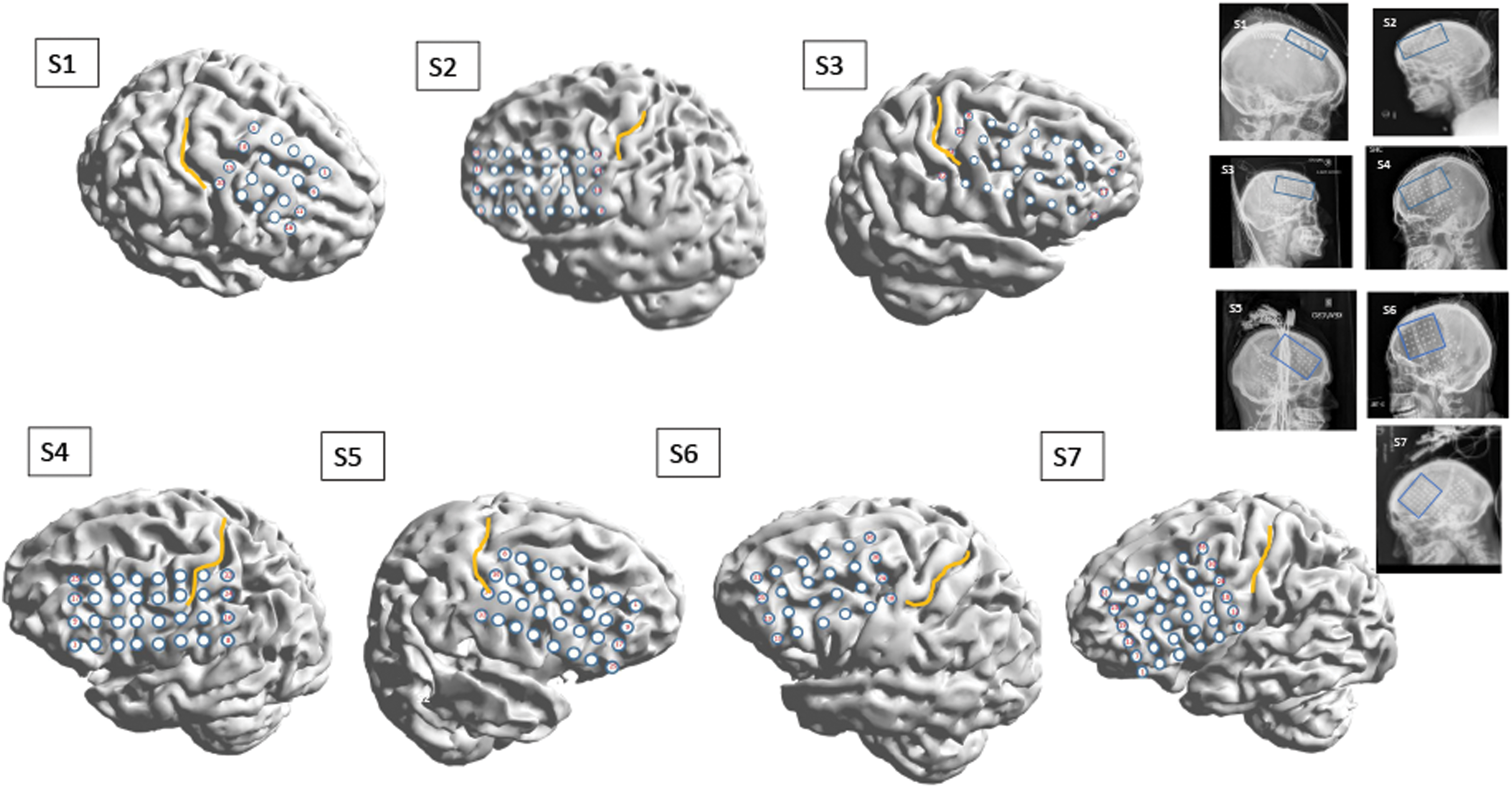
Representations of cortical surfaces of the subject group S1–S7. All surfaces were reconstructed from high-resolution, T1-weighted clinical MRI scans, with subdural electrode positions extracted and superimposed from coregistered postimplant CT scans using CURRY^®. The yellow line marks the central sulcus over each cortical surface. Each subject's postimplant skull X-ray is shown in the group to the right, with the entire subdural implant scheme seen as patterned high-attenuation artifact in each image. The blue rectangles in these images denoted the lateral frontal electrode group (grid), whose recordings provided the data (iEEG) for this work. CT, computed tomography; iEEG, intracranial electroencephalogram; MRI, magnetic resonance imaging. Color images are available online.

Segments of raw ECoG in the resting awake and asleep states were reviewed by the first author, a board-certified electroencephalographer. All data analyzed in this work were from the lateral frontal grid, whose recordings were confirmed to be free of pathological activity (abnormal slowing, spiking, or seizure onsets) for the entirety of the hospitalization. Three or four epochs, each of duration 2–6 min, in the awake and asleep states in machine-derived zero reference montage were archived for offline analysis. Epochs were no closer than 8 h of recording time apart and also more than 4 h before, or following, any seizure; a concurrent review of video suggested the behavioral state as either quiet wakefulness or asleep throughout individual epochs. Offloaded data were preprocessed by resampling to 256 Hz (for subjects S5–S7), notch filtered to eliminate 60 Hz artifact, and normalized to zero mean and unit variance. All data processing was done with custom scripts in MATLAB^®, except where specifically indicated.

The study was approved by the Institutional Review Board of the University of Florida, with the requirement of patient consent waived due to the study's retrospective nature.

Electrode functional connectivity

Functional connectivity between a pair of electrodes for a data epoch was measured with amplitude cross-correlation (ACC), the Pearson correlation of their respective Hilbert amplitudes (Bastos and Schoffelen, 2015). The Hilbert amplitude of a function x(t) is the magnitude of the associated analytic (“quadrature”) function x(t) – iH(x(t)), where H denotes the Hilbert transform and is the envelope of that function (Karl, 1989). For our discrete data x(n), the Hilbert amplitude 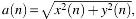where y(n) = H (x(n)) (black line in Fig. 2A, B, E). At time point n, we defined the electrode connectivity (EC) of a certain electrode as the average of its functional connectivity with all the other electrodes of the grid over a 5-sec epoch starting at n. The time dependence of EC was computed in moving windows of 5 sec that overlapped by 4 sec yielding a value of EC every second. We also defined grid connectivity (GC) as the spatial (i.e., across all the electrodes) average of individual ECs. ECs were computed for the entire ECoG signal, as well as for ECoG filtered into the canonical EEG bands (δ [0–4], θ [4–8], α [8–13], β [13–32], γ [ > 32] Hz). To compute EC in a certain EEG band, we decimated the signal such that its bandwidth was higher than the maximum frequency of that band [i.e., we used δ (24), θ (12), α (6), β (3), and γ (1), where the numbers in the parenthesis represent the decimation factors]. We then filtered the decimated signals with low-pass (for the δ band) or band-pass filters (for the θ, α, β, and γ bands). Thus, for band-pass filtered signals, the envelope spectrum was shifted to the origin of the frequency axis (red line in Fig. 2D, F) ensuring that the spectra of the amplitude in all the EEG bands had a “low-pass” shape, similar to the spectrum of the full bandwidth ECoG (Fig. 2B).

FIG. 2.

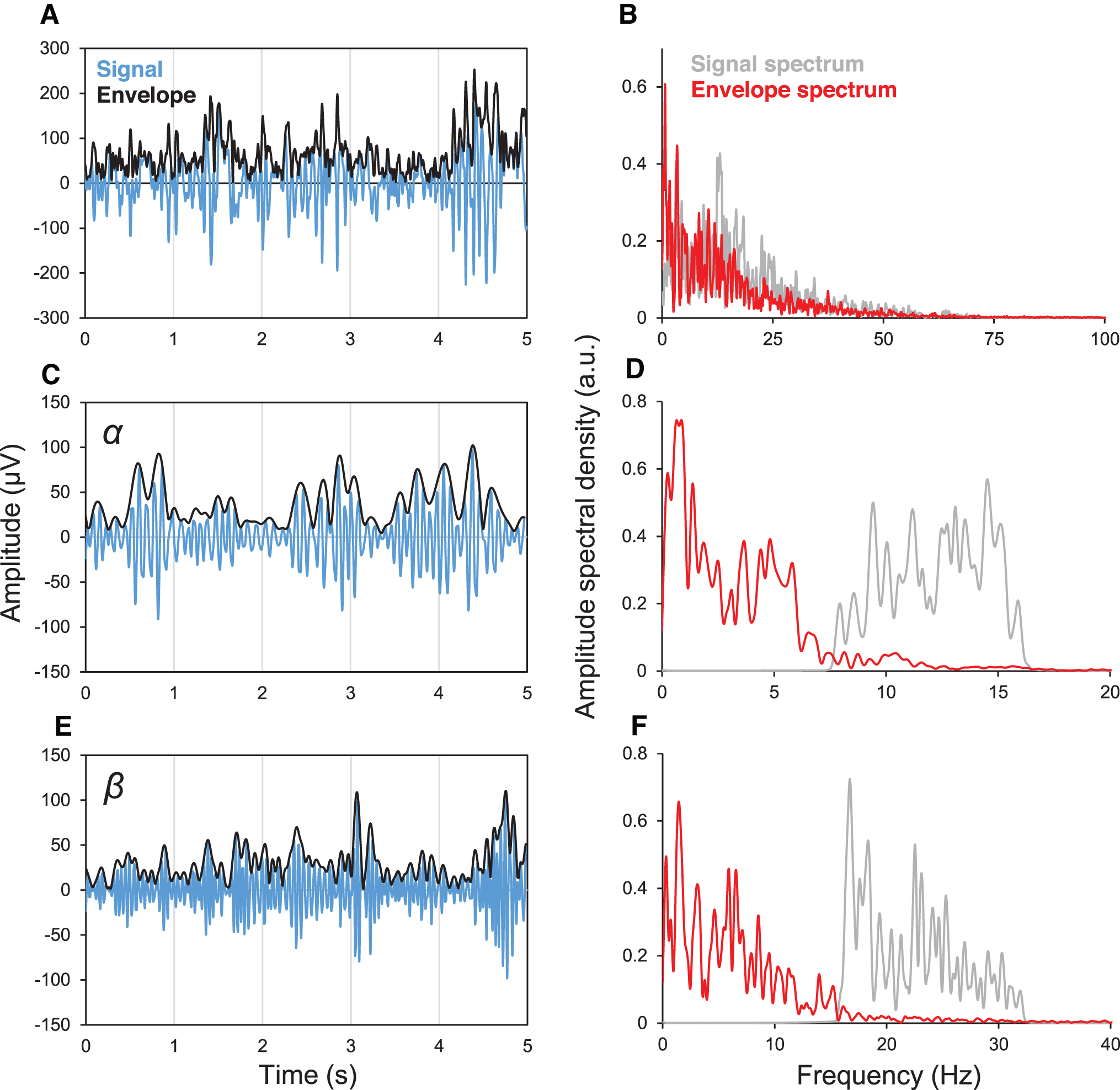
Spectra of a typical iEEG signal and of its linearly filtered versions in the canonical α and β EEG bands and their corresponding envelopes (black lines in A, C, E). (A) iEEG signal (light blue) and its envelope—the amplitude of the analytic signal (see the Methods section)—shown for a time epoch of 5 sec. (B) The amplitude spectral density of the epoch (gray) and of its envelope (red). (C) Filtered signal in α band (light blue) and its envelope. (D) Spectrum of the alpha band-pass filtered signal (gray) and its envelope (red). Computing the envelope demodulates the filtered signal, and the envelope spectrum shifts to the origin. (E) Filtered iEEG signal in beta band (light blue) and its envelope (black). (F) Spectra of the filtered signal (gray) and its envelope (red). EEG, electroencephalogram. Color images are available online.

Electrode sample entropy

Sample entropy (SE) is a measure of signal “complexity” (Richman and Moorman, 2000); small values imply more frequent instances of patterns, recognizable features, or regularity in the data, and large values imply greater randomness, information content, or irregularity. SE is indexed by two parameters m—embedding dimension—an estimate of the length of feature being diagnosed, and r—tolerance—the allowable error between similar features. For a data series of length N, x = {x ₁, x ₂, …, x_N }, one defines a template vector of length m, m « N, x_m (i) = {x_i , x_i _{+ 1}, …, x _{i + m−1}}, and the Euclidean distance |x_m (i) − x_m (j)| (i ≠ j). SE is then −ln (A/B), where A is the number of template vector pairs having |x_m _{+ 1}(i) − x_m _{+ 1}(j) < r and B is the number of template vector pairs having |x_m (i) − x_m (j)| < r. We used the conventional choices of m = 2 and r = 0.2. The SE of an electrode (electrode sample entropy; ESE) was computed from the Hilbert amplitude time series of that electrode. We computed ESE for the full bandwidth ECoG signal as well as the data filtered into EEG bands.

Graph analysis

For each 5-sec time epoch, we computed the M × M ACC connectivity matrix, M being the number of electrodes in the recording grid. All elements of the leading diagonal were set to zero. We then normalized the values of all matrices to lie between 0 and 1 and set to zero entries smaller than a proportion ρ (0.3, 0.45, or 0.6 here) of the largest entries. The normalized and thresholded connectivity matrix was used as the adjacency matrix for the calculation of the following network metrics: average path length (APL), the average of the shortest path between any two graph nodes; clustering coefficient (CC), the geometric mean of all the triangles associated with each node; modularity (MD), the degree to the graph represents nonoverlapping groups of nodes, such that the number of within-group edges is maximized, while minimizing the number of between-group edges. Algorithms for computation of network metrics were adapted from the Brain Connectivity Toolbox (Rubinov and Sporns, 2010).

Statistics

We computed Pearson correlations between ECs and ESEs for the awake and sleep states for each subject. In addition, we computed Pearson correlations between the grid SE (GSE) and GC, as well as APL, CC, and MD time series.

Results

Electrode positions

Figure 1 illustrates the reconstructed positions and size of the lateral frontal grid for all seven patients, projected on to their individual brain surfaces. The yellow line marks the position of the central (Rolandic) sulcus in each case, with the gyri immediately in front and behind it representing the primary motor (M1) and sensory (S1) areas, respectively. The insets are postoperative skull X-rays that show the entire implant scheme, with the rectangles highlighting the lateral frontal contacts that were isolated for the analysis presented here.

Reciprocity of EC and ESE

We computed the mean electrode connectivity (mEC) and mean electrode sample entropy (mESE) for the whole-bandwidth signal and the filtered signal within the canonical EEG bands, for both the wake and sleep states. The means were obtained by time-averaging all the ECs and ESEs corresponding to that electrode from all the records of the condition (see the Methods section). We found that, in general, mEC and mESE were in inverse proportion to each other. The upper left panel of Figure 3A shows the electrode-by-electrode mEC of the whole-bandwidth awake ECoG for subject S3 in descending order (red line). The gray line represents the corresponding mESEs, and the inverse relation is obvious, with Pearson correlation as shown (R = −0.46). The next three panels show a qualitatively similar relation holding for the δ, θ, and α band-passed signals. The inverse relationship apparently breaks down in the β and γ bands (lower panel, middle, and right), although the absolute values of the connectivities in the bands (left y-axis) are small (<0.07), and the range of variability of the sample entropies is much reduced, although their absolute values remain in the O(1) range. Figure 3B shows the same information, for the same electrode order, but in the sleep state. The blue lines show mEC. The inverse relationship between mEC and mESE is stronger than in wakefulness for the whole bandwidth signal and its low-frequency pass bands. Again, the inverse relationship breaks down for the β and γ bands (lower panel, middle, and right) that have small mEC values with smaller range of excursion of mESE, although the latter remains O(1) in absolute value.

FIG. 3.

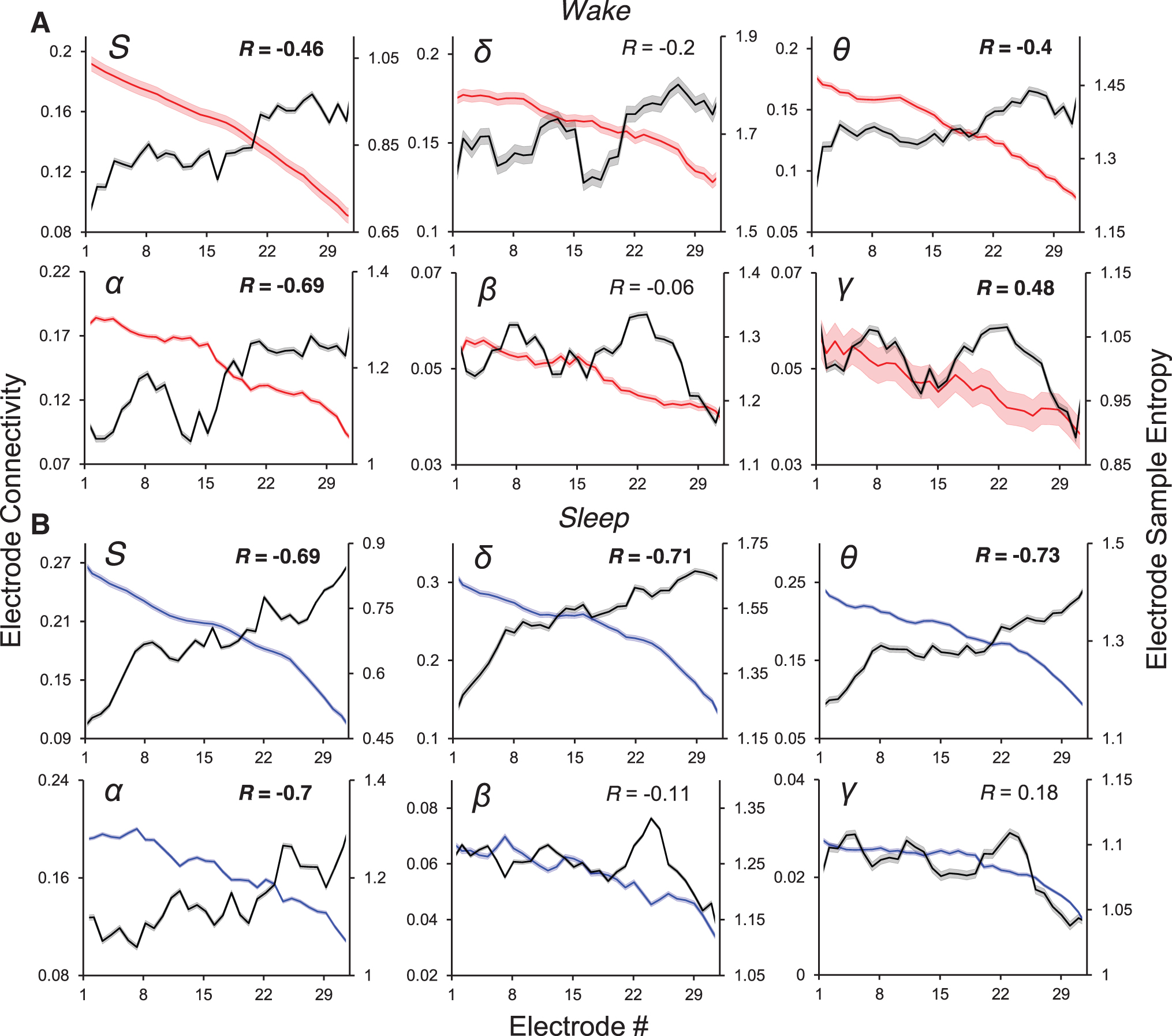
mEC (red—wake; blue—sleep) and mESE (black) for the whole signal (inset S), and in the δ, θ, α, β, and γ bands (corresponding insets), for subject S3. The error shadows in these lines represent the standard error of the mean in estimating these metrics. (A) (Upper left) Values of mECs of the 32-electrode grid sorted in descending order (red). The sample entropy (black) is seen to vary inversely. (Upper middle and right; lower left) With the same electrode order, the mECs and mESEs are shown in the δ, θ, α pass bands; the inverse relationship is seen to hold. (Lower middle and right) Similar plots for the β and γ pass bands show a roughly directly proportional relationship, although the absolute values of the ESE are about a third of those in the higher pass bands. (B) Similar plots for the sleep state. The anticorrelations between mEC and mESE are stronger, with higher R values for the whole signal and its δ, θ, α pass bands. ESE, electrode sample entropy; mEC, mean electrode connectivity; mESE, mean electrode sample entropy. Color images are available online.

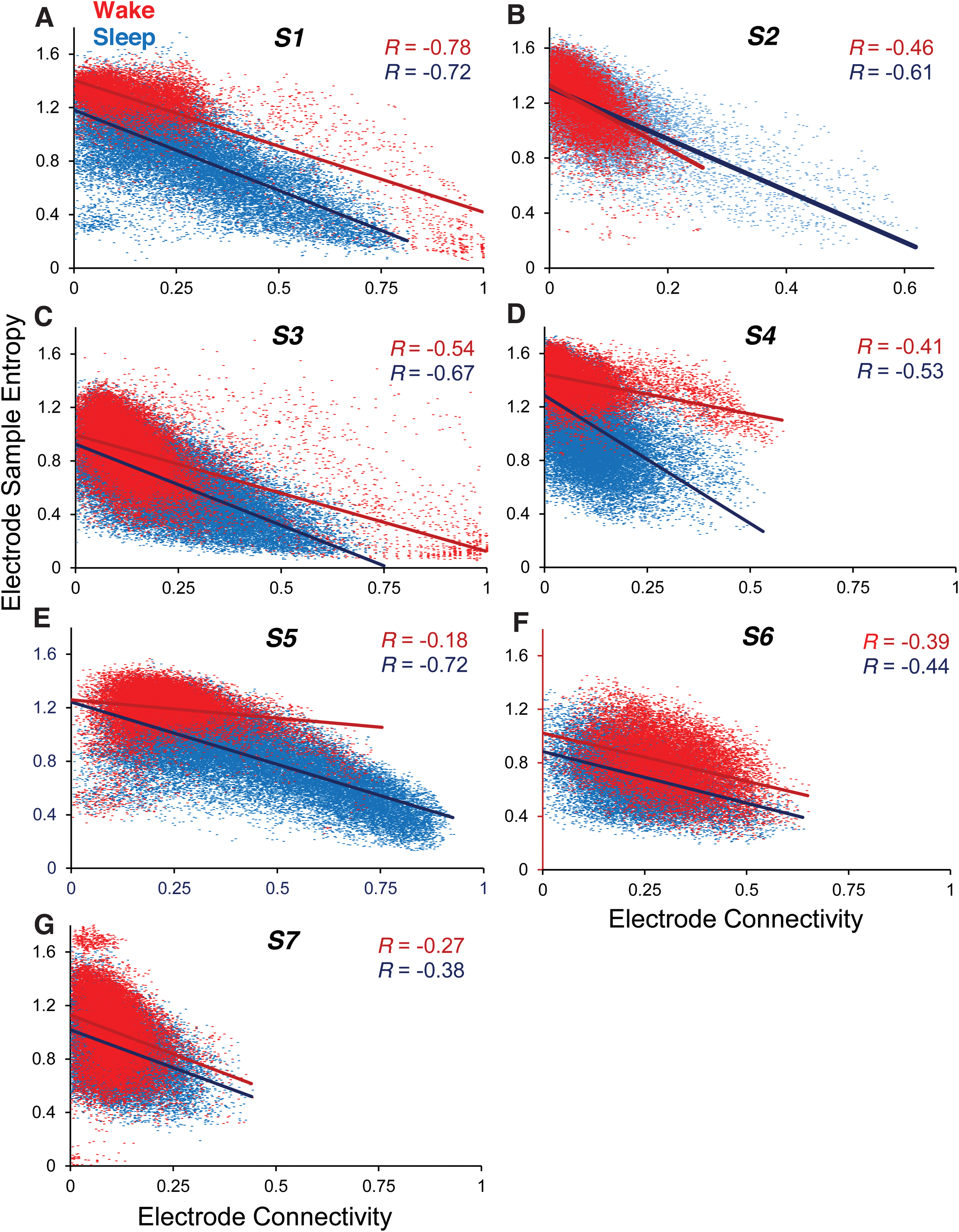
Figure 4 shows all values of EC and ESE for all subjects S1–S7. For these, only the full bandwidth signals were used. Each separate figure consists of two scatter plots, one each for the wake (red) and sleep (blue) conditions. Each dot represents the ordered pair (ESE, EC) values for a single 5-sec epoch. Given that ESE and EC were computed every second for every electrode (see the Methods section), the number of data points in each scatter plot (≈18,000 being a typical value) is the number of seconds in the concatenated (awake or asleep) data multiplied by the number of electrodes. The inverse relationship between ESE and EC is clear in every case, with a trend for the effect to be larger in the sleep state, with the R value in the seven subjects in the wake and sleep states being S1: −0.78, −0.72; S2: −0.46, −0.61; S3: −0.54, −0.67; S4: −0.41, −0.53; S5: −0.18, −0.72; S6: −0.39, −0.44; and S7: −0.27, −0.38.

FIG. 4.

(A–G) Scatter plots of all the pairs (EC, ESE) computed from the wake (red) and sleep (blue) states for all the subjects S1–S7, together with regression lines and Pearson correlations R between EC and ESE for the wake (red) and sleep (blue) states. Color images are available online.

Extrema of mEC and mESE; rostrocaudal gradients

Figure 5 is a heat map of the mEC-mESE results for subject S2, for the full bandwidth signal. The disposition of the frontal grid electrodes is redrawn from this subject's reconstructed lateral brain surface (Fig. 1), with the central sulcus marked in yellow. The color bar scale is individualized for each image to maximize contrast. Figure 5A and B shows the maps of connectivity in the wake and sleep states, which are seen to be highly congruent. The reciprocal relationship between mEC and mESE is clearly seen in the sleep state (compare Fig. 5B and D), where areas of heat and cold literally “exchange places” on the brain surface. This reciprocal relationship is present, but somewhat less precise, in the wake state (compare Fig. 5A and C). The eight electrode contacts at the posterior portion of the grid have the lowest (highest) mECs (mESEs) of all, and these are seen to be overlying the lower peri-Rolandic sensorimotor cortex.

FIG. 5.

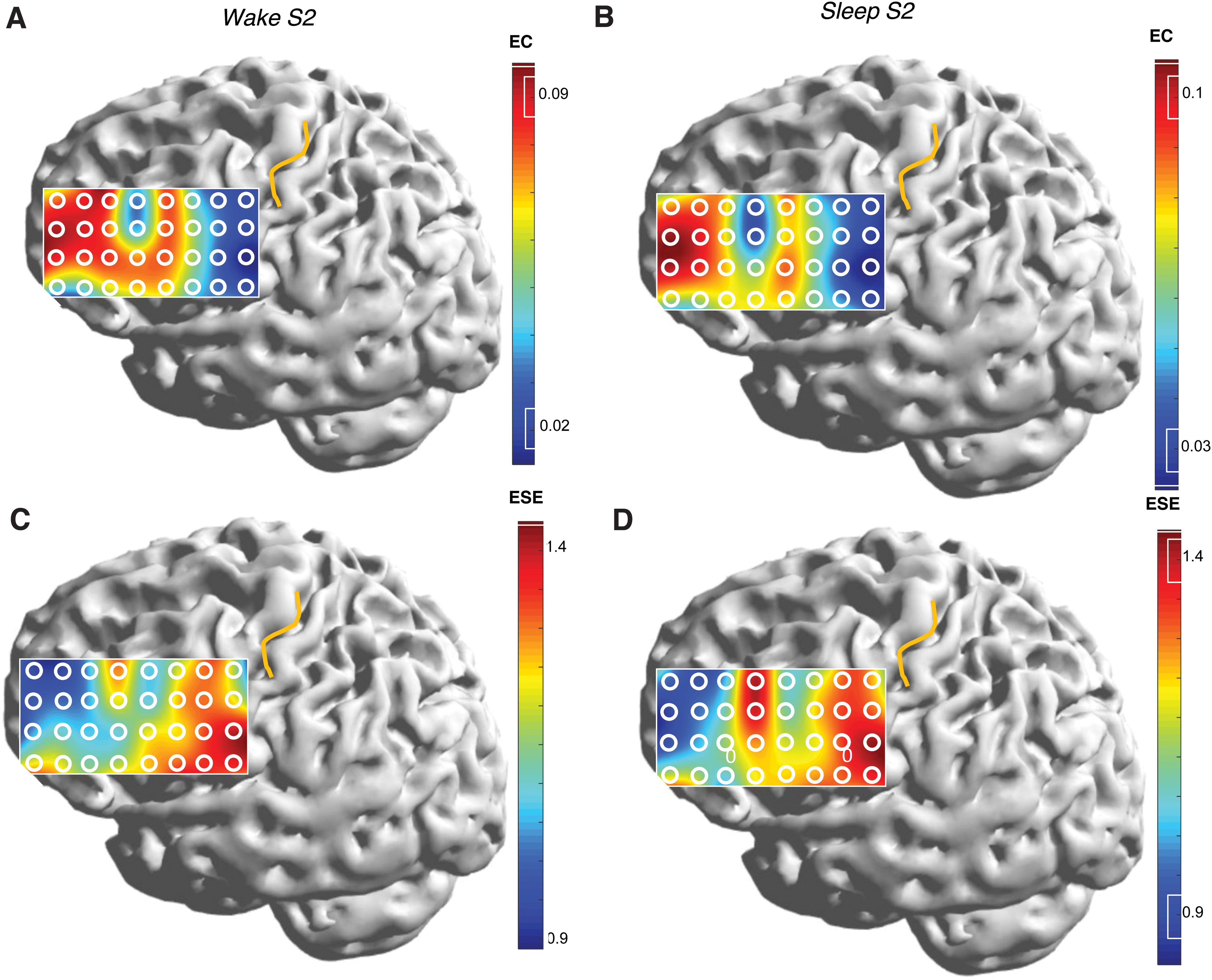
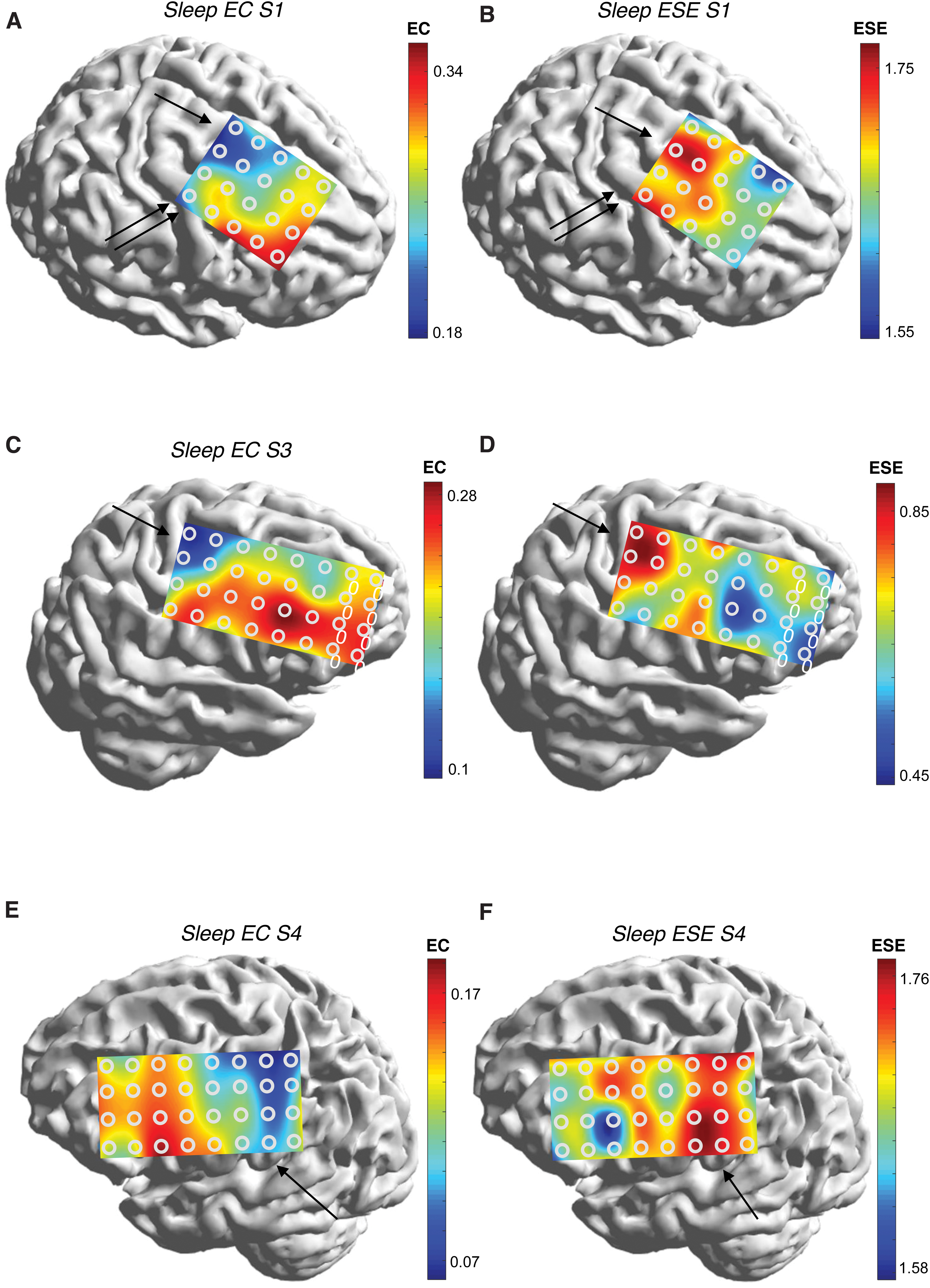
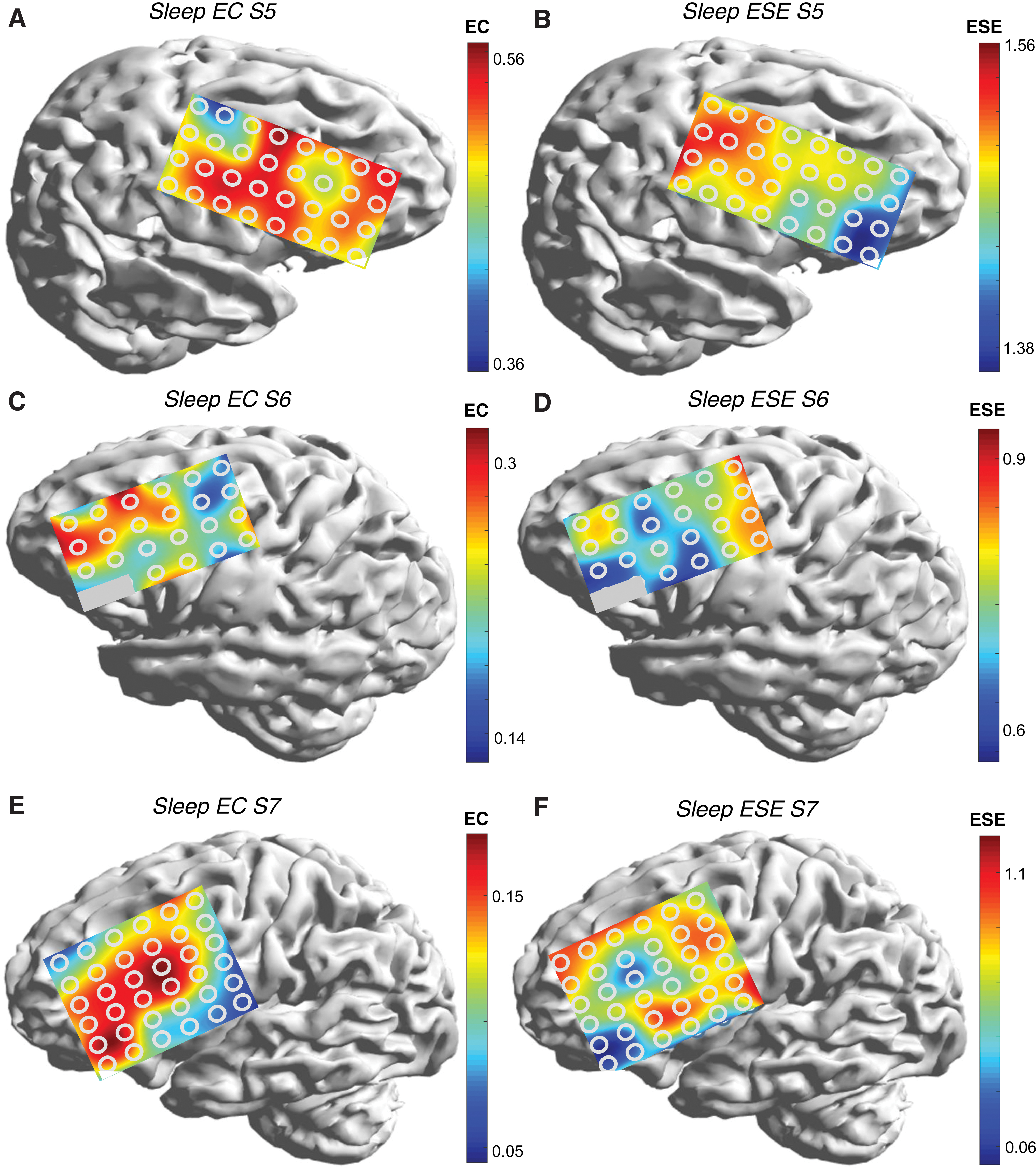
Heat maps showing the spatial variation of mEC and mESE over the lateral frontal cortex of subject S2. Wake states are to the left, and sleep states to the right. Top-down comparisons (A–C) and (B–D) reveal a reciprocal relationship between mEC and mESE with areas of heat and cold showing a complementary relationship. This reciprocal relationship is particularly vivid in the sleep state, but also clearly appreciated in wakefulness. In addition, electrodes overlying or in closest proximity to the Rolandic area (the posterior two columns of electrodes) have the lowest (highest) mEC (mESE) values. Color images are available online.

Figures 6 and 7 are mEC-mESE heat maps in the sleep state for the remainder of the subjects. The positions of the central sulcus are not shown for clarity, but may be inferred from comparison with Figure 1. Comparing left and right maps (Figs. 6A and B, 6C and D, 6E and F, 7A and B, 7C and D, and 7E and F), the reciprocal relationship between mEC and mESE is appreciated in every case. It is also clear that electrodes overlying or in closest proximity to the Rolandic area have the lowest (highest) mEC (mESE) values. In S1, the posterior end of the frontal grid is mostly anterior to the precentral gyrus; yet, mEC is highest in the posterior electrode contacts, especially superiorly (arrow), and also at the single electrode comprising the left bottom corner, as the precentral gyrus curves forward to underlie that electrode (double arrow). The heat map of mESE follows the opposite color trend. In S3, the extrema of mEC/mESE are seen in the posterior upper segment of grid that overlies the superior Rolandic region (arrow). In S4, a similar picture to S2 is seen (arrow); indeed, there is a hint of the extrema falling off in the electrodes that extend posterior to the sensory strip. In S5, the extremum of mEC appears in the upper left of the grid that overlies the primary motor cortex (arrow). The extremum is less pronounced along the rest of the posterior edge of the grid, although the mESE map shows the longitudinal extent of the extremum more clearly (arrow). S6 shows the extremum of ESE vertically along the posterior margin of the grid, with a pronounced minimum over the anteroinferior border, similar to subjects S2–S5 and S7. In S7, the extremum in EC is seen at the lower right corner, corresponding to the lower portion of the motor strip (arrows).

FIG. 6.

(A–F) Heat maps showing the spatial variation of mEC and mESE over the lateral frontal cortex in the sleep states of subjects S1, S3, and S4. The position of the central sulcus may be inferred by comparison with Figure 1. In S1, mEC is highest in the posterior electrode contacts, especially superiorly (arrow) and also at the single electrode comprising the left bottom corner, as the precentral gyrus curves forward to underlie that electrode (double arrow). The heat map of mESE follows the reciprocal trend. In S3, the extrema of mEC/mESE are seen in the posterior upper segment of grid that overlies the superior Rolandic region (arrow). In S4, a similar picture to S2 is seen (arrow), with a hint of the extrema falling off in the electrodes that extend posterior to the sensory strip. Color images are available online.

FIG. 7.

(A–F) Similar to Figure 6, for subjects S5, S6, and S7. In S5, the extremum of mEC appears in the upper left of the grid that overlies the primary motor cortex (arrow). The extremum is less pronounced along the rest of the posterior edge of the grid, although the mESE map shows the longitudinal extent of the extremum more clearly (arrow). S6 shows the extremum of ESE vertically along the posterior margin of the grid, with a pronounced minimum over the anteroinferior border, similar to subjects S2–S5 and S7. In S7, the extremum in EC is seen at the lower right corner, corresponding to the lower portion of the motor strip (arrows). Color images are available online.

The extreme values of mEC and mESE over the Rolandic region were part of a more general rostrocaudal gradient observed in all patients, with larger (smaller) values of mEC (mESE) occurring anteriorly. A particularly compelling example is S2 (Fig. 5).

Dynamic behavior; network metrics

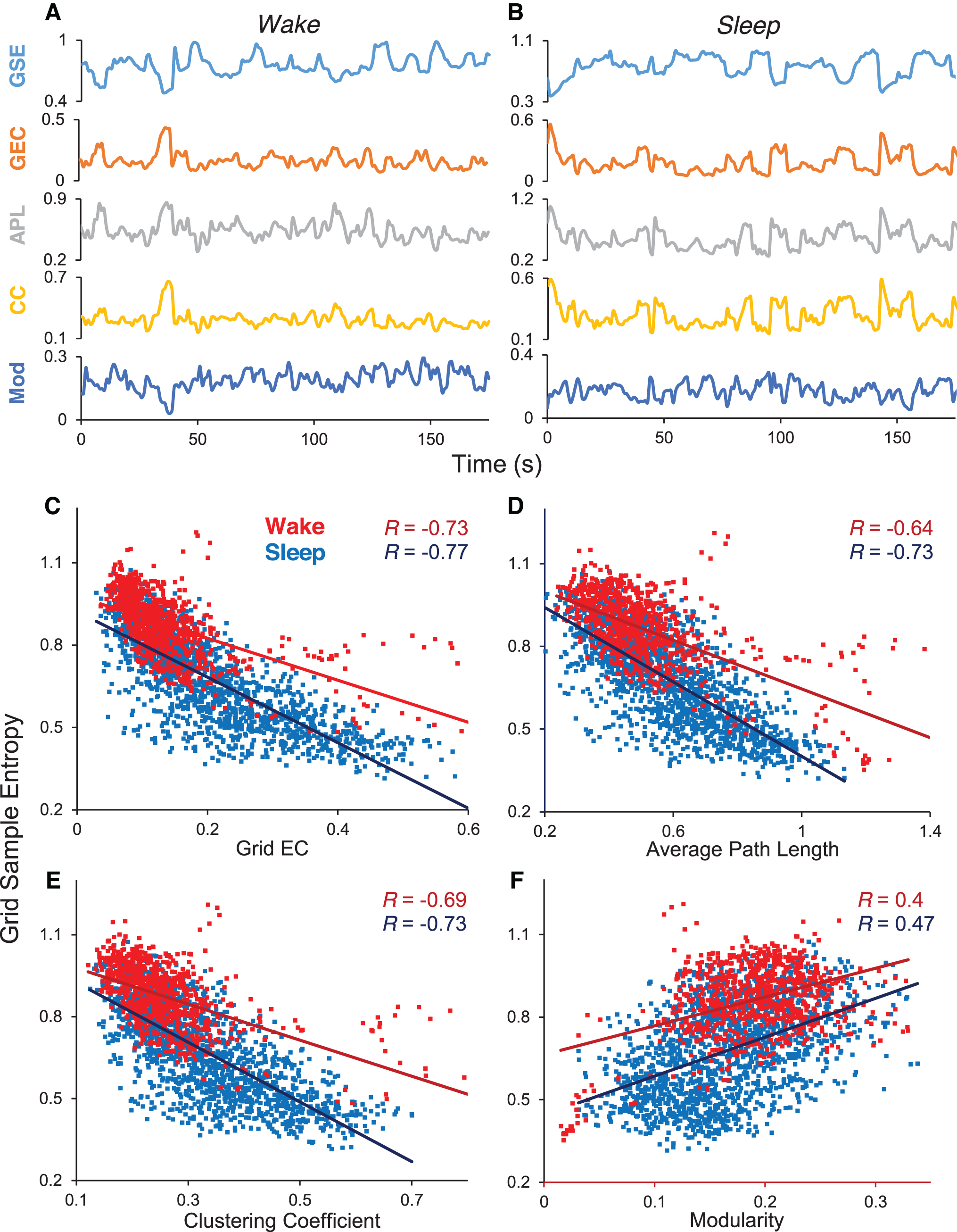
We explored whether the inverse relationship described above was also dynamic: that is, whether the reciprocity was true only in a time-averaged sense, or whether moment-to-moment changes in EC were reflected in a reciprocal manner in ESE. For this, we used the spatial average of SE and EC, obtaining the quantities of GSE and grid electrode connectivity (GEC; see the Methods section). Figure 8A and B shows that the inverse relationship was true dynamically. The top two traces in Figure 8A (wake) and Figure 8B (sleep) are time series of GSE and GEC in subject S3 for an ∼175-sec epoch. The anticorrelation of the two time series is visually obvious. The bottom three time series in Figure 8A and B show that, in addition, the network metrics of APL and CC are in phase with GEC, but modularity (MD) is in antiphase. Figure 8C–F shows the scatter plots of all the data for this subject. Each dot represents the ordered pair (GSE, GEC) value for a single 5-sec epoch in the concatenated (awake or asleep). The number of data points in each scatter plot is the number of seconds in concatenated (awake or asleep) data (≈600 being a typical value). The anticorrelation of GSE with GEC, APL, and CC, and the correlation with MD is demonstrated separately for the wake and sleep states. Table 2 shows these results in numerical form for all the subjects S1–S7, for three different values of graph analysis threshold.

FIG. 8.

(A, B) Concurrent time series of GSE (the average value of ESE over the grid), GEC (the average value of EC over the grid), as well as the network metrics of APL, CC, and MD, for an example wake (A) and a sleep (B) epoch in subject S3. The GSE and GEC were computed every second for moving time epochs of 5 sec, overlapping by 4 sec. The graph measures (APL, CC, MD) were created from adjacency matrices of time epochs (see the Methods section). GSE is negatively correlated with GEC, APL, and CC, but positively correlated with MD. (C–F) Clusters of the pairs (GEC, GSE), (APL, GSE), (CC, GSE), and (MD, GSE) computed from all the wake (red) and sleep (blue) data epochs from subject S3. Each point in the clusters represents a pair corresponding to a single time epoch. High negative correlations are seen between GSE and GEC, GSE and APL, and GSE and CC, and positive correlations are seen between GSE and MD. APL, average path length; CC, clustering coefficient; GEC, grid electrode connectivity; GSE, grid sample entropy; MD, modularity. Color images are available online.

Table 2.

Correlation Between Grid Sample Entropy and Grid Connectivity and Graph Measures for All Subjects S1–S7, for Three Different Values of Graph Analysis Threshold

	Cortical state	R(GC, GSE)	R(APL, GSE)	R(CC, GSE)	R(MD, GSE)
ρ = 0.3
S1	Sleep	−0.869	−0.799	−0.822	0.416
S1	Wake	−0.929	−0.829	−0.866	0.327
S2	Sleep	−0.837	−0.5	−0.748	0.403
S2	Wake	−0.444	−0.173	−0.351	0.307
S3	Sleep	−0.775	−0.712	−0.719	0.426
S3	Wake	−0.726	−0.570	−0.676	0.393
S4	Sleep	−0.602	−0.6	−0.606	0.039
S4	Wake	−0.674	−0.577	−0.638	0.509
S5	Sleep	−0.844	0.711	−0.758	0.384
S5	Wake	−0.670	−0.367	−0.526	0.283
S6	Sleep	−0.526	−0.455	−0.422	0.061
S6	Wake	−0.619	−0.335	−0.426	0.149
S7	Sleep	−0.549	−0.554	−0.543	0.330
S7	Wake	−0.614	−0.559	−0.549	0.184
ρ = 0.45
S1	Sleep	−0.869	−0.867	−0.864	0.464
S1	Wake	−0.929	−0.831	−0.911	0.562
S2	Sleep	−0.837	−0.630	−0.740	0.401
S2	Wake	−0.444	−0.207	−0.302	0.284
S3	Sleep	−0.775	−0.733	−0.733	0.468
S3	Wake	−0.726	−0.637	−0.691	0.399
S4	Sleep	−0.602	−0.535	−0.585	0.037
S4	Wake	−0.674	−0.612	−0.636	0.518
S5	Sleep	−0.844	−0.766	−0.773	0.372
S5	Wake	−0.670	−0.462	−0.543	0.292
S6	Sleep	−0.526	−0.446	−0.433	0.075
S6	Wake	−0.619	−0.404	−0.436	0.148
S7	Sleep	−0.549	−0.518	−0.549	0.356
S7	Wake	−0.614	−0.551	−0.570	0.231
ρ = 0.6
S1	Sleep	−0.869	−0.866	−0.868	0.523
S1	Wake	−0.929	−0.879	−0.923	0.572
S2	Sleep	−0.837	−0.683	−0.727	0.406
S2	Wake	−0.444	−0.220	−0.276	0.282
S3	Sleep	−0.775	−0.724	−0.734	0.502
S3	Wake	−0.726	−0.669	−0.696	0.415
S4	Sleep	−0.602	−0.464	−0.551	0.106
S4	Wake	−0.674	−0.634	−0.639	0.560
S5	Sleep	−0.844	−0.775	−0.782	0.404
S5	Wake	−0.670	−0.475	−0.538	0.305
S6	Sleep	−0.526	−0.421	−0.434	0.108
S6	Wake	−0.619	−0.431	−0.441	0.220
S7	Sleep	−0.549	−0.457	−0.535	0.367
S7	Wake	−0.614	−0.522	−0.568	0.266

ρ, proportional threshold for graph analysis; APL, average path length; CC, clustering coefficient; GC, grid connectivity; GSE, grid sample entropy; MD, modularity; R(,), Pearson correlation of the quantities in the parenthesis.

Discussion

Multimodality mapping of the brain offers an equivalent number of perspectives on the neural structure and function. The accumulation of diverse data sets and metrics also raises the question of their synthesis. Scalp EEG was arguably the first “brain mapping” technology to ever appear; yet, the availability of normative atlases for whole-brain iEEG is recent (Frauscher et al., 2018; von Ellenrieder et al., 2020). These atlases have in turn prompted efforts that turn the raw data into visualizable brain maps (Kalamangalam et al., 2020). Here we move away from a descriptive account to instead relate to the character of rhythm from a particular location (judged by its SE, a “univariate” behavior) to its neighborhood connectivity (judged by its average connectivity to other electrodes, a “multivariate” behavior). Our larger aim was to link some aspects of the local dynamics—the iEEG at a cortical location—to an aspect of its neurobiology—its connectivity to other cortical areas. The lateral frontal lobe was chosen due to its relatively large and confluent extent of electrode coverage and the absence of pathological findings in the iEEG as judged by conventional visual analysis.

Our first observation was that local SE, computed from the iEEG at a single electrode, was inversely related to that electrode's average connectivity to other regions (Figs. 3, 4, and 8). That is, the local degree of order (or disorder) reflected connectivity to nonlocal elements. Our second observation was of an anterior/posterior (or rostrocaudal) gradient in the magnitude of the ESE, with lower entropies anteriorly, over the anterior frontal regions, and higher entropies posteriorly, over the peri-Rolandic regions. Being inversely related, EC followed the opposite gradient (Figs. 5 –7). These observations were true for the signal in its entire bandwidth, and also the signal filtered into the lower (δ, θ, and α) pass bands. Finally—and in keeping with our hypothesis of the primary and association cortical areas being somehow different with respect to iEEG—highest entropies (and lowest connectivities) were all over the primary sensorimotor (peri-Rolandic) cortex. We discuss each of these findings in turn.

Our hypothesis that temporal change at a given brain location, judged by a suitable local metric—SE here—would be related to how it connected to other locations, judged by another suitable metric—averaged ACC here—was purely heuristic. Essentially, a central thesis of modern neuroscience—perhaps harking back to Sherrington (1942)—is that connectivity underlies function, at both the structural and functional levels (Friston, 2011; Kelso, 1995). As a corollary, iEEG at a brain location would presumably be influenced by its wider network of connections: aspects of the network would be reflected, or diagnosable, from activity at just a single location. Alternatively, one might invoke the spirit of Takens' theorem in physical dynamics (Takens, 1981): under conditions of nondegeneracy, observations of just a single variable that participates in a larger system of interacting variables are sufficient to reconstruct the dynamics of the full system. Thus, considering a particular single brain location as a “variable,” we expected its dynamic features to provide diagnostic information on the wider network—the multivariable interacting system—it was part of. Specifically, we hypothesized that a highly connected electrode might be more “constrained” in the diversity of its behavior than a sparsely connected one.

SE (and its variants) is a widely used measure of temporal diversity (or “complexity”) in biological time series (Richman and Moorman, 2000); to compute connectivity, we devised the metric of an electrode-wise connectivity, and indeed found the hypothesized inverse relationship between the two. We are aware of studies in the cardiovascular field (Costa et al., 2005; Pincus, 2006) that argue for the relationship between connectedness and entropy in reverse. That is, greater regularity (low entropy) is thought to imply greater subsystem autonomy, and thus disconnectedness from coupling and control mechanisms. We believe both interpretations could be valid, depending on the nature of the system: that is, the particular dynamics of the variable involved and the pattern of coupling. For instance, a self-oscillating system, say the signal from a small cortical region generating an intrinsic rhythm, when connected to sources of neural noise, might indeed exhibit more entropy when coupled, than when in a free-running mode. On the contrary, a cortical region with highly complex intrinsic dynamics and exhibiting wide-band, noise-like, signals might decrease its entropy when networked to a regularly oscillating external influence. Indeed, our results in the faster frequency bands were different from the behavior of the low-frequency pass bands and hinted at this reverse relationship (Fig. 3). A closer examination of the differing behavior of low-frequency and high-frequency rhythms in our data set, however, awaits further work. Thus, the stronger conclusion from our present results is not that entropy and connectivity are related inversely, but that they are related at all.

Our results have similarities to a number of resting-state (rs) functional MRI (fMRI) studies on brain connectivity and local brain oxygen-level dependent (BOLD) signal entropy. Shafei et al. (2019) analyzed whole-brain rs-fMRI in conditions of dopamine depletion and normalcy in a large normal cohort, finding that brain regions that exhibited increased entropy in the dopamine-depleted condition also had reduced their connectivities. Using data from the Human Connectome Project (HCP) (Van Essen et al., 2013), McDonough and Nashiro (2014) found a variable relationship between BOLD signal complexity and functional network connectivity—with a negative correlation at fine spatial scales and a positive correlation at large scales. On the contrary, Wang et al. (2018) report positive correlations between functional connectivity and multiscale entropy in a variety of contexts—simulated neural mass models, an animal model with simultaneous fMRI and electrophysiological recordings, and rs-fMRI from the HCP. Reconciling these disparities—which may be one or more of system, modality, or technique specificity—remains a task for the future.

Our observation of a rostrocaudal gradient in SE and EC is consistent with current notions regarding the anatomical and functional parcellation of the lateral frontal lobe. The grid implant on subject S3, for instance (Fig. 6), shows 32 electrodes arranged in a 4 × 8 array. The region of coverage would correspond to portions of Brodmann/Walker areas 3, 4, 6, 8Ad, 8Av, 44, 45A, 45B, 9/46d, 9/46d, 9, 46, 47/12, and 10 (Petrides and Pandya, 1999), corresponding to primary motor, primary sensory, premotor, frontal eye field, inferior frontal gyrus (Broca's area in the dominant hemisphere), dorsolateral prefrontal cortex, ventrolateral prefrontal cortex, and frontal pole (Nieuwenhuys et al., 2008). The functions attributed to these brain areas (primary areas excepted) are broadly those regarded as especially human: the capacity for abstract thought and the faculties of language, reason, and imagination. Thus, “distance away” in the rostral direction from primary areas has been shown to correspond to functional capacities at higher levels of abstraction (Badre and D'Esposito, 2009), such as motor tasks that progressively increase their sophistication (Amiez and Petrides, 2018). In another demonstration of the frontal lobe rostrocaudal axis, Thiebaut de Schotten et al. (2017) studied 59 normals (12 of whom were part of the HCP repository). Using diffusion-weighted magnetic resonance tractography, they identified 12 connectivity-based regions (CBRs) in the frontal lobe from frontal pole to the pre-Rolandic area. These CBRs were found to lie on an anteroposterior axis with respect to measures of cortical thickness (thicker anteriorly), cortical myelin quantification (T1/T2 ratio; lower myelin content anteriorly), and cell body density (smaller cells, less densely packed anteriorly). Their entropy calculations from resting-state fMRI demonstrated highest entropies anteriorly, which they took to indicate higher levels of dendritic and synaptic complexity. The latter results are at variance with ours, but as alluded to, these differences may be modality specific and can only be resolved by studying patients who undergo both rs-fMRI and iEEG.

In exploring the relationship between EEG metrics at a single location (SE) and that location's functions, we surmised that the primary sensorimotor areas might behave differently from association areas (premotor and prefrontal brain areas). In the von Economo classification (Nieuwenhuys et al., 2008), the primary motor cortex possesses archetypal agranular cytoarchitecture—prominent pyramidal cell layers with a relative deficit of cellularity in the granular cell layers. Primary sensory cortex is the archetype granular cortex, with sparse pyramidal cellularity and abundant cellularity in the granular layers. Primary sensory areas are also the only neocortical areas that possess excitatory interneurons. Primary areas are among the earliest to myelinate and distinguished from the other von Economo types of association cortices that vary along the classic six-layered architectural template and are late-myelinating (Nieuwenhuys et al., 2008). On the contrary, the prefrontal cortex is a high-order heteromodal area that receives input from all unimodal and heteromodal sensory areas. It possesses a cellularity characterized by dense two-way reciprocally connected cells. Prefrontal pyramidal neurons also exhibit a persisting activity following activation cues, thought to represent the neurophysiological correlate of working memory. These enumerated differences between the primary and association areas of the frontal lobe are reasons to suspect that an average local field potential signature (i.e., iEEG) would be also different.

We point out that our lumping the primary motor and sensory areas together under the title “Rolandic cortex” is linguistic shorthand only. The differences in cellular architecture and connectivity patterns between the primary motor and sensory areas are considerable and would be expected to, based on this study's hypothesis, yield distinguishable EEG rhythms. The reason we have included both areas under the single umbrella of “Rolandic” is the estimated error in our localization of the subdural electrodes (≈0.5 cm) in any direction, and the fact that the linear dimension of the receptive field of standard clinical subdural macroelectrodes is 0.3–0.5 cm (Kahane and Dubeau, 2014), features sufficient to introduce uncertainty in our labeling of a particular electrode contact as definitely recording from primary motor or primary sensory. It is clear also that our results demonstrate heterogeneity of mEC and mESE within the frontal association regions, with the suggestion of a variable superoinferior gradient within the premotor and prefrontal regions (Figs. 5 –7). Some of these latter issues, in addition to taking account of hemispheric dominance and handedness, are items for further study.

It may appear redundant for us to introduce an EEG-based metric that diagnoses primary sensorimotor brain areas, when the association of the mu (μ) rhythm with its peri-Rolandic location has long been known (Gastaut, 1952). We point out though that our iEEG diagnostic is entirely independent of the μ rhythm, and has arisen from a hypothesis-driven approach with regard to connectivity and entropy, features not detectable by visual analysis. In addition, iEEG studies confirm that the μ rhythm disappears in sleep (Arroyo et al., 1993), whereas our demonstrated entropy-connectivity gradients are in fact clearer in sleep, degrading somewhat in wakefulness. A closer examination (Figs. 5 –7) reveals that the degradation is due to the entropy map changing its spatial structure, whereas the connectivity map remains relatively static. We have extended these observations to situations where the subjects are active—moving their hands, looking around, or talking—and entropy maps degrade further but connectivity maps remain relatively static (data not shown). The relative robustness of mEC maps is therefore noteworthy, and may reflect underlying structural (“hard-wired”) cortical connectivity (Abdelnour et al., 2018; Honey et al., 2009; Mars et al., 2018). It is also clear that the inverse mEC-mESE relationship operates in real-time, as confirmed by following whole GSE and GEC in time, where the temporal relationship between the two (Fig. 8) and the network metrics of APL, CC, and MD are also shown.

We reiterate that our judgment of sleep and wakefulness was informal, based on video review, time of day, and the qualitative appearances of the iEEG. Formal sleep staging requires scalp EEG coverage (AASM, 2007; Rechtschaffen and Kales, 1968) that is possible with subdural grid patients, but was not available for this patient group. Thus, our identification of the sleep and wake states must be considered approximate. However, the consistently differing appearances of mEC and mESE in the wake and sleep states suggest that this distinction was made with reasonable accuracy. With regard to identifying the central sulcus, none of the patients underwent stimulation mapping to identify the primary motor cortex due to a lack of clinical necessity for the procedure. Thus, the central sulcus was identified by anatomical landmarks only. Anatomical localization is, however, known to be sufficiently accurate in the absence of gross brain malformations (Naidich and Yousry, 2007), as was the case in our patient group.

We finally comment on several technical issues. First, we chose to study the iEEG in human patients in a restricted brain region judged to be normal in retrospect (rather than whole-head scalp EEG in a normal population) due to the former's fine spatial scale and excellent signal-to-noise ratio. A comparison with scalp EEG is of interest, although we believe that magnetoencephalography (MEG) would be the ideal noninvasive alternative signal source, due to the finer spatial sampling of conventional MEG recordings and the lack of attenuation of magnetic fields by skull and soft tissues (Hari, 2011). Our data stream was in referential montage, with the reference being a machine-specified nonbiological “zero” potential. The choice of reference can be crucial for the proper use and interpretation of quantitative EEG metrics (Shirhatti et al., 2016); our choice of machine zero excluded confound from reference contamination. Our computation of connectivity obviously only involved brain areas over which recording contacts were present; brain underlying a particular recording contact might have had its most significant connections outside the grid, and not represented in the calculation. However, “short” connections vastly outnumber “long” connections in the brain (Shepherd, 2004), and our estimate of a single electrode's connectivity to other electrodes was, on average, likely close to the ideal of including all possible connections of that electrode. Our estimates of mEC (although not mESE) would admittedly suffer inaccuracies at the edge electrodes and corner electrodes. Confounds due to edge effects cannot be entirely excluded in our data, although such effects would not explain the anteroposterior gradients observed. In addition, several instances of maxima and minima of mEC appeared completely enclosed within the individual grids (Figs. 5 –7), indicating that edge effects were not a major influence on these. On a different point, we point out that the paradox of analysis of “normative” data from patients with epilepsy is one that has no possible resolution. Our data come from patients with intracranial electrodes that were distant from areas of spiking, pathological slowing, or seizure onset, and therefore judged “normal” by experienced clinicians. However, the effects of epilepsy syndrome, duration of epilepsy, and medications cannot be fully discounted, and the question of whether the results indeed apply to a normal population is raised. However, given our data source, and that prolonged iEEG data will never be available from a normative population, it is unclear how the above paradox can ever be resolved.

In conclusion, we demonstrate that brain networks do imply brain dynamics. Specifically, we have shown that the entropy of the averaged field potential over a given brain location, at the spatial scale of subdural macroelectrodes, and at the temporal resolution of clinical recordings, is (inversely) related to that location's connectivity to other brain regions. Applied to the lateral frontal lobe, these metrics demonstrate a rostrocaudal topography that clearly identifies differences between the primary sensorimotor and frontal association cortex. These findings add to the documented evidence regarding a rostrocaudal axis to the organization in the human frontal lobe. Although novel, our work admittedly does not address the classical empiricisms of frontal lobe EEG, for example, the mu rhythm and diffuse beta frequencies characteristic of the Rolandic and frontocentral brain areas (Hari, 2011). Drawing these electrophysiological threads together will be key to better understanding why brain rhythms over the frontal lobe appear the way they do.

Footnotes

Acknowledgments

We thank the technicians and nurses at the UFHealth Neuromedicine Hospital Epilepsy Monitoring Unit for their role in patient care and data collection. We acknowledge the neurosurgical expertise of Steven Roper, MD, in patient management. We thank Alexander Cerquera, PhD, for generating some preliminary results on our data. We thank Michael Okun, MD, Thomas Mareci, DPhil, and members of the Gunduz laboratory at the University of Florida for their encouragement.

Authors' Contributions

G.P.K. conceived the study and wrote the article. M.I.C. performed data analysis and cowrote the article.

Author Disclosure Statement

Neither of the authors has a conflict of interest to declare.

Funding Information

The authors acknowledge support from the Wilder Family Endowments to the University of Florida.

References

Abdelnour

, Dayan

, Devinsky

, et al. 2018. Functional brain connectivity is predictable from anatomic network's Laplacian eigen-structure. Neuroimage, 172:728–739.

American Academy of Sleep Medicine (AASM). 2007. The AASM Manual 2007 for the Scoring of Sleep and Associated Events: Rules, Terminology and Technical Specifications. Westchester, IL: American Academy of Sleep. Medicine.

Amiez

, Petrides

. 2018. Functional rostro-caudal gradient in the human posterior lateral frontal cortex. Brain Struct Funct, 223:1487–1499.

Arroyo

, Lesser

, Gordon

, et al. 1993. Functional significance of the mu rhythm of human cortex: an electrophysiologic study with subdural electrodes. Electroencephalogr Clin Neurophysiol, 87:76–87.

Badre

, D'Esposito

. 2009. Is the rostro-caudal axis of the frontal lobe hierarchical?. Nat Rev Neurosci, 10:659–669.

Bastos

, Schoffelen

. 2015. A tutorial review of functional connectivity analysis methods and their interpretational pitfalls. Front Syst Neurosci, 9:175.

Berger

. 1929. Uber das Elektrenkephalogramm des Menschen [On the electroencephalogram of man]. Arch Psych Nervenkrankheiten, 87:527–570.

Costa

, Goldberger

, Peng

. 2005. Multiscale entropy analysis of biological signals. Phys Rev E Stat Nonlin Soft Matter Phys, 71:021906.

Frauscher

, von Ellenrieder

, Zelmann

, et al. 2018. Atlas of the normal intracranial electroencephalogram: neurophysiological awake activity in different cortical areas. Brain, 141:1130–1144.

10.

Friston

. 2011. Functional and effective connectivity: a review. Brain Connect, 1:13–36.

11.

Gastaut

. 1952. Electrocorticographic study of the reactivity of the rolandic rhythm. Rev Neurol (Paris), 87:176–182.

12.

Hari

. 2011. Magnetoencephalography: methods and applications In: Schomer DL, Lopes da Silva FH (eds.) Niedermeyer's Electroencephalography. Philadephia: Lippincott Williams & Wilkins; pp. pp. 865–900.

13.

Honey

, Sporns

, Cammoun

, et al. 2009. Predicting human resting-state functional connectivity from structural connectivity. Proc Natl Acad Sci U S A, 106:2035–2040.

14.

Kahane

, Dubeau

. 2014. Intracerebral depth electrode electroencephalography. In: Ebersole JS (ed.) Current Practice of Clinical Electroencephalography. Philadelphia: Wolters Kluwer; pp. 393–441.

15.

Kalamangalam

, Long

, Chelaru

. 2020. A neurophysiological brain map: spectral parameterization of the human intracranial electroencephalogram. Clin Neurophysiol, 131:665–675.

16.

Karl

. 1989. Introduction to Digital Signal Processing. Cambridge, MA: Academic. Press.

17.

Kelso

JAS

. 1995. Dynamic Patterns: The Self-Organization of Brain and Behavior. Cambridge, MA: MIT. Press.

18.

Mars

, Passingham

, Jbabdi

. 2018. Connectivity fingerprints: from areal descriptions to abstract spaces. Trends Cogn Sci, 22:1026–1037.

19.

McDonough

, Nashiro

. 2014. Network complexity as a measure of information processing across resting-state networks: evidence from the Human Connectome Project. Front Hum Neurosci, 8:409.

20.

Naidich

, Yousry

. 2007. Functional neuroanatomy. In: Stippich C (ed.) Clinical Functional MRI. Berlin: Springer; pp. 53–86.

21.

Nieuwenhuys

, Voogd

, Van Huizen

. 2008. Telencephalon: neocortex In: The Human Central Nervous System . Berlin: Springer-Verlag; pp. 491–680.

22.

Petrides

, Pandya

. 1999. Dorsolateral prefrontal cortex: comparative cytoarchitectonic analysis in the human and the macaque brain and corticocortical connection patterns. Eur J Neurosci, 11:1011–1036.

23.

Pincus

. 2006. Approximate entropy as a measure of irregularity for psychiatric serial metrics. Bipolar Disord, 8:430–440.

24.

Rechtschaffen

, Kales

. 1968. A Manual of Standardized Terminology, Techniques and Scoring System for Sleep Stages in Human Subjects. Los Angeles: BIS/BRA. UCLA.

25.

Richman

, Moorman

. 2000. Physiological time-series analysis using approximate entropy and sample entropy. Am J Physiol Heart Circ Physiol, 278:H2039–H2049.

26.

Rubinov

, Sporns

. 2010. Complex network measures of brain connectivity: uses and interpretations. Neuroimage, 52:1059–1069.

27.

Shafiei

, Zeighami

, Clark

, et al. 2019. Dopamine signaling modulates the stability and integration of intrinsic brain networks. Cereb Cortex, 29:397–409.

28.

Shepherd

. 2004. Neocortex. In: Shepherd GM (ed.) The Synaptic Organization of the Brain. New York: Oxford University Press; pp. 499–558.

29.

Sherrington

. 1942. Man on His Nature. Cambridge, England: Cambridge University. Press.

30.

Shirhatti

, Borthakur

, Ray

. 2016. Effect of reference scheme on power and phase of the local field potential. Neural Comput, 28:882–913.

31.

Takens

. 1981. Detecting strange attractors in turbulence. In: Rand DA, Young L-S (eds.) Dynamical Systems and Turbulence . Berlin: Springer-Verlag; pp. 366–381.

32.

Thiebaut de Schotten

, Urbanski

, Batrancourt

, et al. 2017. Rostro-caudal architecture of the frontal lobes in humans. Cereb Cortex, 27:4033–4047.

33.

Van Essen

, Smith

, Barch

, et al. 2013. The WU-Minn Human Connectome Project: an overview. Neuroimage, 80:62–79.

34.

von Ellenrieder

, Gotman

, Zelmann

, et al. 2020. How the human brain sleeps: direct cortical recordings of normal brain activity. Ann Neurol, 87:289–301.

35.

Wang

DJJ

, Jann

, Fan

, et al. 2018. Neurophysiological basis of multi-scale entropy of brain complexity and its relationship with functional connectivity. Front Neurosci, 12:352.