Seizure Frequency Is Associated with Effective Connectivity of the Hippocampal–Diencephalic–Cingulate in Epilepsy with Unilateral Mesial Temporal Sclerosis

Abstract

Background:

Temporal lobe epilepsy (TLE) with mesial temporal sclerosis (MTS) is a common intractable epilepsy. To seek neural correlates of seizure recurrence, this study investigated aberrant intrinsic effective connectivity (iEC) in TLE with unilateral MTS and their associations with seizure frequency.

Methods:

Thirty patients with unilateral MTS (left/right MTS = 14/16) and 37 age-matched healthy controls underwent resting-state functional magnetic resonance imaging (rsfMRI) on a 3-Tesla magnetic resonance imaging (MRI) system. The structural equation modeling was employed to estimate the iEC of the three candidate epilepsy models, including the Papez circuit, hippocampal–diencephalic–cingulate (HDC) model, and simplified HDC model. After comparing the performance of model fitting, the best model was selected to compare iEC among the study groups. The linear regression analysis was performed to associate abnormal iEC with seizure frequency.

Results:

The simplified HDC model was the best model to estimate iEC across the three study groups (p < 0.05), and it composed of the 26 interconnected pathway between the mesial temporal lobe, thalamus, and cingulate cortices. The linear regression analysis revealed a significant relationship between the shared iEC alterations in both patient groups and seizure frequency (adjusted-R ² = 0.350; p = 0.037), including the three paths of mammillary body (MB) → bilateral anterior thalamic nuclei (left: standardized β-value = 0.580, p = 0.013; right: standardized β-value = −0.711, p = 0.006) and right hippocampus → MB (standardized β-value = 0.541, p = 0.045).

Conclusions:

Our findings provide new insights into neurophysiological significance relevant to seizure recurrence. Aberrant iEC on the neural paths connected to the MB can be a potential imaging marker, aiding the therapeutic management in TLE with unilateral MTS.

Impact statement

Within the simplified hippocampal–diencephalic–cingulate model, we identified that altered intrinsic effective connectivity (iEC) on the three paths connecting to the mammillary body was common in temporal lobe epilepsy (TLE) with left and right mesial temporal sclerosis (MTS) and was associated with seizure frequency. Therefore, these common iEC alterations could be a potential imaging marker, aiding the therapeutic management in patients with TLE with unilateral MTS.

Introduction

Approximately one third of patients with epilepsy do not benefit from adequate seizure control with antiepileptic medication (Kwan and Brodie, 2000). Temporal lobe epilepsy (TLE) with mesial temporal sclerosis (MTS) is the most common intractable epilepsy (Wiebe and Jette, 2012), but brain regions causing recurrent seizures remain unclear. A recent meta-analysis of associations of seizure frequency with progressive brain atrophy in TLE with MTS suggested that recurrent seizure is attributed to cumulative brain damage (Caciagli et al., 2017). The atrophic brain structures could extend beyond the hippocampus (HP) and included the temporal lobe, cingulum, thalamus, and other subcortical regions. Recent resting-state functional magnetic resonance imaging (rsfMRI) studies reported that compared with patients with infrequent seizures, patients with frequent seizures exhibited decreased functional connectivity between brain regions in the medial temporal lobe and locations remote from seizure focus (Bharath et al., 2015; Pressl et al., 2019). These brain areas with structural and functional abnormalities were hypothesized to be related to seizure recurrence in TLE with MTS (Bernhardt et al., 2009; Bharath et al., 2015; Pressl et al., 2019).

Although functional connectivity analysis demonstrated seizure-related brain dysfunctions in a local seizure focus (Lee et al., 2014) and different epileptogenic networks (Laufs et al., 2006) in TLE, such an analytic method lacks the directionality of information flow between brain regions. Hence, several rsfMRI studies turned to intrinsic effective connectivity (iEC) analyses, which described the strength of intrinsic directional information flow between brain regions at rest, to investigate how epileptic activity affects iEC (Ji et al., 2013; Park et al., 2018). To investigate the effect of seizure frequency on iEC, Park et al. (2018) compared iEC within the mesial temporal region between TLE patients with better seizure control and TLE patients with poor seizure control. They found that aberrant iEC observed in patients with poor seizure control was affected by seizure frequency. However, the aberrant iEC within a brain-wise network relevant to TLE with MTS and its association with seizure recurrence still remains unclear.

The Papez circuit, which is a set of neuronal pathways linking the HP to the mammillary body (MB), anterior thalamic nuclei (ATN), cingulate gyrus, parahippocampal gyrus (PHG), and back to the HP (Papez, 1937), has been implicated in seizure generation and propagation (Laxpati et al., 2014). Moreover, with the recent development of anterograde and retrograde tract-tracing techniques, the past neurophysiological studies (Aggleton et al., 2014, 2015; Bubb et al., 2017) on the rat and macaque monkey brains have characterized more afferent and efferent projections from each brain area of the Papez circuit compared with the directional pathways initially described by Papez (1937). For instance, the connection between the ATN and posterior cingulate gyrus (PCG) is reciprocal (Bubb et al., 2017), whereas the connection between the ATN and PCG in the Papez circuit is unidirectional (Papez, 1937). These directed connections comprise a redefined neural model named the hippocampal–diencephalic–cingulate (HDC) model (Bubb et al., 2017).

To make HDC model less complex and more understandable, Bubb et al. (2017) further proposed the simplified version of HDC model, where the interconnections were common between both the rat and monkey HDC models and were assumed to exist in the human memory circuitry, providing parallel efferent information from the posterior mesial temporal lobe (both hippocampal and parahippocampal regions) to the cingulate cortex and thalamus. Thus, the HDC model and its simplified version may be more appropriate than the Papez circuit to explore aberrant iEC in TLE patients with unilateral MTS and to clarify the relationships between aberrant iEC and seizure frequency.

The present study performed structural equation modeling (SEM) (Lin et al., 2009; McIntosh et al., 1994) to evaluate iEC within the Papez circuit, HDC model, and simplified HDC model in the study groups. SEM is a robust mathematical technique in which data covariance describing causal relationships between the brain regions of a predefined brain network model is used to estimate iEC (Inman et al., 2012). Although there are other methods to estimate iEC, such as dynamic causal modeling (Friston et al., 2014) and Granger causality analysis (Ji et al., 2013), we employed SEM owing to its robustness and efficiency for estimating iEC. Given that rsfMRI data are the spontaneous blood oxygen level–dependent (BOLD) signal derived from intrinsic brain activity, Inman et al. (2012) suggested that SEM analysis can efficiently refer causal relationships between the brain regions of a predefined model without prior knowledge of causal relationships obtained from specific cognitive tasks. To date, SEM analysis has been widely applied to study aberrant directional information flow in various neurodegenerative disorders at rest or during a cognitive task, providing potential imaging markers of brain diseases (Inman et al., 2012; Rowe et al., 2002).

Therefore, this study aimed to identify iEC alterations, which were both shared by two subtypes of TLE (i.e., TLE with left MTS and TLE with right MTS) and associated with seizure frequency. Specifically, we performed SEM analysis for rsfMRI BOLD signals to fit three candidate models (Papez circuit, HDC network, and simplified HDC network) and selected the best-fitted one. We predicted that the HDC or simplified HDC model would fit rsfMRI BOLD signals better than the Papez circuit because the HDC or simplified HDC models have relatively more directed connections. The best-fitted model was used to identify shared iEC alterations in both patients with left and right MTS. We hypothesized that some of shared iEC alterations would be correlated with seizure frequency, indicating the significance of neurophysiology underlying seizure recurrence in TLE with unilateral MTS.

Materials and Methods

Participants

We recruited 30 patients with unilateral MTS (left/right MTS = 14/16) and 37 healthy controls from 2010 to 2016 (Table 1). All patients underwent comprehensive clinical assessments based on the current International League Against Epilepsy classification (Fisher et al., 2017), including structural magnetic resonance imaging (MRI) examinations, long-term clinical video-electroencephalography (EEG) monitoring, and detailed interviews. The seizure onset at the unilateral or bilateral temporal lobes was assessed by the long-term clinical video-EEG recording, whereas the side of MTS in TLE patients was identified according to MRI findings. The MRI features were diagnosed by one experienced neurologist (H.-H.L.) and two neuroradiologists, including: (1) evidence of MTS or hippocampal sclerosis showing the presence of brain atrophy in the mesial temporal lobe or HP on T1-weighted imaging and abnormal signal hyperintensity in the mesial temporal region on T2-weighted imaging on the epileptic side, and (2) absence of other structural abnormalities beyond the ipsilateral temporal lobe, such as bilateral MTS, trauma, tumors, or gray matter heterotopia. We additionally used a Computational Anatomy Toolbox with LPBA40 human brain atlas based on SPM12 (Wellcome Trust Center for Neuroimaging, London, United Kingdom) to process T1-weighted images to calculate hippocampal volume on two hemispheres for each study group (Table 1). Participants who had a previous history of brain surgery or other neurological or psychiatric disease were excluded to avoid the potential influence of brain atrophy.

Table 1.

Demographic Data of Patients with Left and Right Temporal Lobe Epilepsy with Mesial Temporal Sclerosis and Healthy Controls

	Left MTS (n = 14)	Right MTS (n = 16)	Healthy controls (n = 37)	Equality of means	p-Value
	Mean (standard deviation)			Equality of means	p-Value
Age (years)	38.21 (9.33)	38.63 (9.00)	37.86 (8.89)	F _2,64 = 0.042	0.959
Gender (female/male)	7/7	8/8	17/20	—	—
Handedness (right/left)	(14/0)	(16/0)	(37/0)	—	—
Epilepsy duration (years)	24.00 (8.31)	26.56 (11.33)	—	t _2,28 = 0.810	0.425
Onset age (years)	14.29 (6.47)	12.25 (7.18)	—	t _2,28 = −0.697	0.492
Seizure frequency (number per month)	2.01 (1.79)	1.78 (2.54)	—	t _2,28 = 0.277	0.784
Seizure type (subject number)
FAS only	0	2	—	—
FIAS only	12	13	—	—
FBTCS	2	1	—	—
Engel classification
Class II	0	3	—	—	—
Class III	8	8	—	—	—
Class IV	6	5	—	—	—
Number of AEDs (subject number)
1 AED	2	0	—	—
2 AEDs	2	4	—	—
3 AEDs	8	11	—	—
4 AEDs	2	1	—	—
Hippocampal volume (cm³)
Left HP	3.12 (0.60)^a	3.68 (0.40)	3.79 (0.24)	F _2,64 = 15.90	<0.001
Right HP	3.87 (0.33)	3.08 (0.95)^a	3.89 (0.26)	F _2,64 = 14.25	<0.001

Post hoc analysis shows a significant reduction in hippocampal volume. Compared with healthy controls, the left MTS group had a significant reduction in the left hippocampal volume, and the right MTS group had a significant reduction in the right hippocampal volume; two unilateral MTS groups had no significant reduction in the contralateral hippocampal volume.

AED, antiepileptic drug; FAS, focal awareness seizure; FBTCS, focal to bilateral tonic–clonic seizure; FIAS, focal impaired awareness seizure; HP, hippocampus; MTS, mesial temporal sclerosis.

All patients were drug-resistant TLE. The information with regard to seizure frequency was obtained from seizure diaries and interviews of patients and their family members. This study was approved by the local Research Ethics Committee of the National Taiwan University Hospital, and written informed consent was obtained from all participants before recruitment (Institutional Review Boards number: 201003009R).

Data acquisition

All MRI data were acquired using a 3-Tesla MRI system (Tim Trio; Siemens, Erlangen, Germany) with a 32-channel phased-array head coil. MRI examinations included high-resolution T1-weighted imaging, T2-weighted imaging, and 6-min rsfMRI. T1-weighted imaging was performed using a 3D magnetization-prepared rapid gradient-echo sequence with the following parameters: repetition time (TR)/echo time (TE) = 2000/3 msec, flip angle = 9 degrees, field of view (FOV) = 256 × 192 × 208 mm³, and matrix size = 256 × 192 × 208. T2-weighted imaging with the axial acquisition plane was performed using a turbo spin-echo sequence with the following parameters: TR/TE = 5920/101 msec, flip angle = 150 degrees, FOV = 256 × 256 mm², matrix size = 256 × 256 × 34, and voxel size = 1 × 1 × 3 mm³.

The 6-min rsfMRI was performed using a gradient echo echo-planar-imaging sequence with the following parameters: TR/TE = 2000/24 msec, flip angle = 90 degrees, FOV = 256 × 256 mm², matrix size = 64 × 64 × 34, voxel size = 4 × 4 × 3 mm³, and 180 volumes per acquisition. All the participants were instructed to close their eyes, relax, and let their mind freely wander during the entire course of rsfMRI scanning.

Data preprocessing

The preprocessing of rsfMRI data was conducted using an rsfMRI data analysis toolbox (Yan and Zang, 2010) based on SPM 12 (Wellcome Trust Center for Neuroimaging), namely the data-processing assistant for rsfMRI (State Key Laboratory of Cognitive Neuroscience and Learning, Beijing Normal University, Beijing, China). The preprocessing procedure began with slice timing and motion corrections. T1-weighted images were coregistered to the mean rsfMRI data and were subsequently segmented into gray matter, white matter, and cerebrospinal fluid by using the unified segmentation algorithm (Yan and Zang, 2010). Segmented T1-weighted images from our study cohort were used to produce a study-specific template by using the diffeomorphic anatomical registration through exponential lie algebraic normalization method (Ashburner, 2007). The study-specific template, which was a tissue probability map, was then normalized to the standard tissue probability map in the Montreal Neurological Institute (MNI) space with T1-weighted contrast to write normalization parameters. The motion-corrected rsfMRI volumes were spatially normalized to MNI space with 3 × 3 × 3 mm isotropic voxel size by the normalization parameters, and spatial smoothing was performed using a 6-mm full-width-at-half-maximum Gaussian kernel. Subsequently, we performed nuisance regression using the following regressors: linear detrending, head motion of six rigid body parameters and framewise displacements (Power et al., 2012), and averaged signals from the white matter and the cerebrospinal fluid. Finally, rsfMRI data were filtered using a bandpass filter (0.008–0.09 Hz) (Fox et al., 2005).

To minimize the impact of rsfMRI data sets with severe head motion on the analysis, we included participants whose averaged framewise displacements of rsfMRI BOLD signals were smaller than 0.5 mm (Power et al., 2012). No participants were excluded based on this criterion. There were no significant differences in the mean standardized temporal signal-to-noise ratios (Krüger et al., 2001) of rsfMRI data among regions of interest (ROIs) in each study groups (Supplementary Fig. S1).

SEM analysis

SEM enables the determination of causality between brain areas by estimating whether the predefined model-implied data covariance matrix supports the observed data covariance matrix. We constructed three causal models with directional paths, namely the Papez circuit, HDC model, and simplified HDC model (Fig. 1A–C) and respectively evaluated the applicability of the three models to our rsfMRI data sets. The directional paths and the corresponding ROIs in the Papez circuit are as follows: HP→MB, MB→ATN, ATN→anterior cingulate gyrus (ACG), ACG→PCG, PCG→PHG, PHG→HP, left ACG↔right ACG, left PCG↔right PCG, left PHG↔right PHG, and left HP↔right HP, where → and ↔ denote unidirectional and bidirectional paths, respectively. All ROIs were obtained from the Talairach Daemon atlas in the MNI space (Fig. 1D, E) (Lancaster et al., 2000). Because of their small size and proximity, the bilateral MBs were merged as a single ROI. An ROI of the PCG partly overlapped with the retrosplenial cortex (Brodmann area 29 and 30), a key hub connecting the cingulate gyrus with PHG (Wei et al., 2017).

FIG. 1.

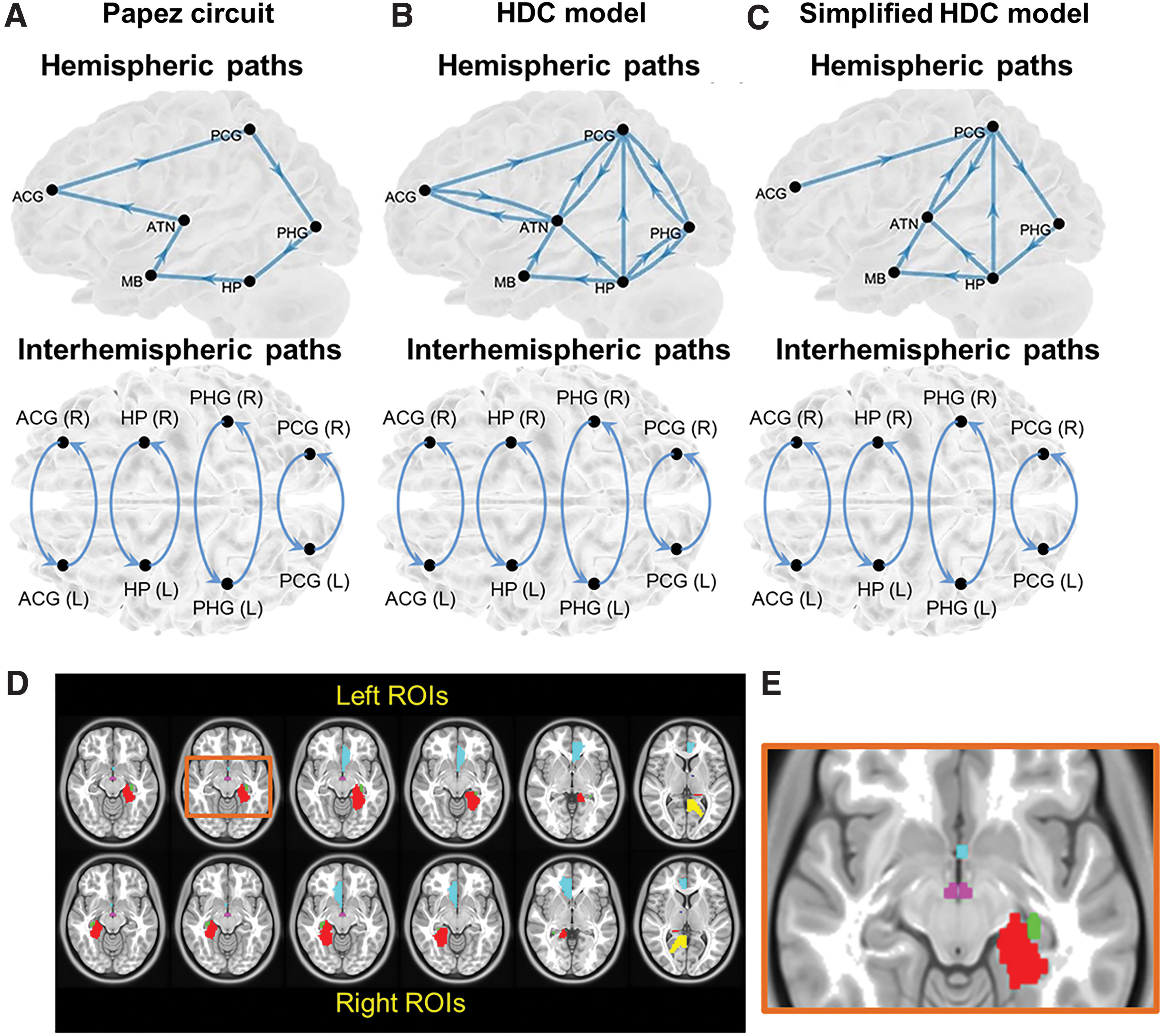
The three candidate neural models proposed to describe the hippocampal transmission, including (A) Papez circuit, (B) HDC model, and (C) simplified HDC model. (D) ROIs of the three models were obtained from the Talairach Daemon atlas in the MNI space. (E) The brown window indicates the anatomical locations of the left HP (green ROI) and MB (purple ROI). Cyan ROI: ACG, blue ROI: ATN, green ROI: HP, purple ROI: MB, red ROI: PHG, yellow ROI: PCG. ACG, anterior cingulate gyrus; ATN, anterior thalamic nuclei; HDC, hippocampal–diencephalic–cingulated; HP, hippocampus; MB, mammillary body; MNI, Montreal Neurological Institute; PCG, posterior cingulate gyrus; PHG, parahippocampal gyrus; ROIs, regions of interest. Color images are available online.

Supplementary Table S1 lists the volume size of all ROIs. Bubb et al. (2017) stemmed from the HDC model with dense and intermediate projections in the macaque monkey brain and noted that the connections ATN↔ACG, ATN↔PCG, PCG↔PHG, and PHG↔HP of the HDC model are reciprocal (Fig. 1B). Considering the important role of the HP in the posterior mesial temporal lobe in human memory circuitry, the simplified version of the HDC model was formed based the removal of the connections ATN↔ACG, HP→PHG, and PHG→PCG (Bubb et al., 2017; Dillingham et al., 2015; Xiang and Brown, 2004). The rest of connections constituted the simplified version of HDC model (Fig. 1C).

SEM analysis procedures are described as follows (Fig. 2). First, rsfMRI BOLD signals were preprocessed and extracted from the selected ROIs. The extracted signals were used to construct an observed covariance matrix for each participant. The observed covariance matrices of a group of participants were averaged to produce a mean observed data covariance matrix Φ. We produced three mean observed covariance matrices from the healthy controls, patients with left MTS, and those with right MTS, respectively. Second, we proposed an anatomically informed model based on each of the Papez circuit, HDC model, and simplified HDC model to construct the model-implied data covariance matrix C, which was represented by the following formulation (McArdle and McDonald, 1984):

FIG. 2.

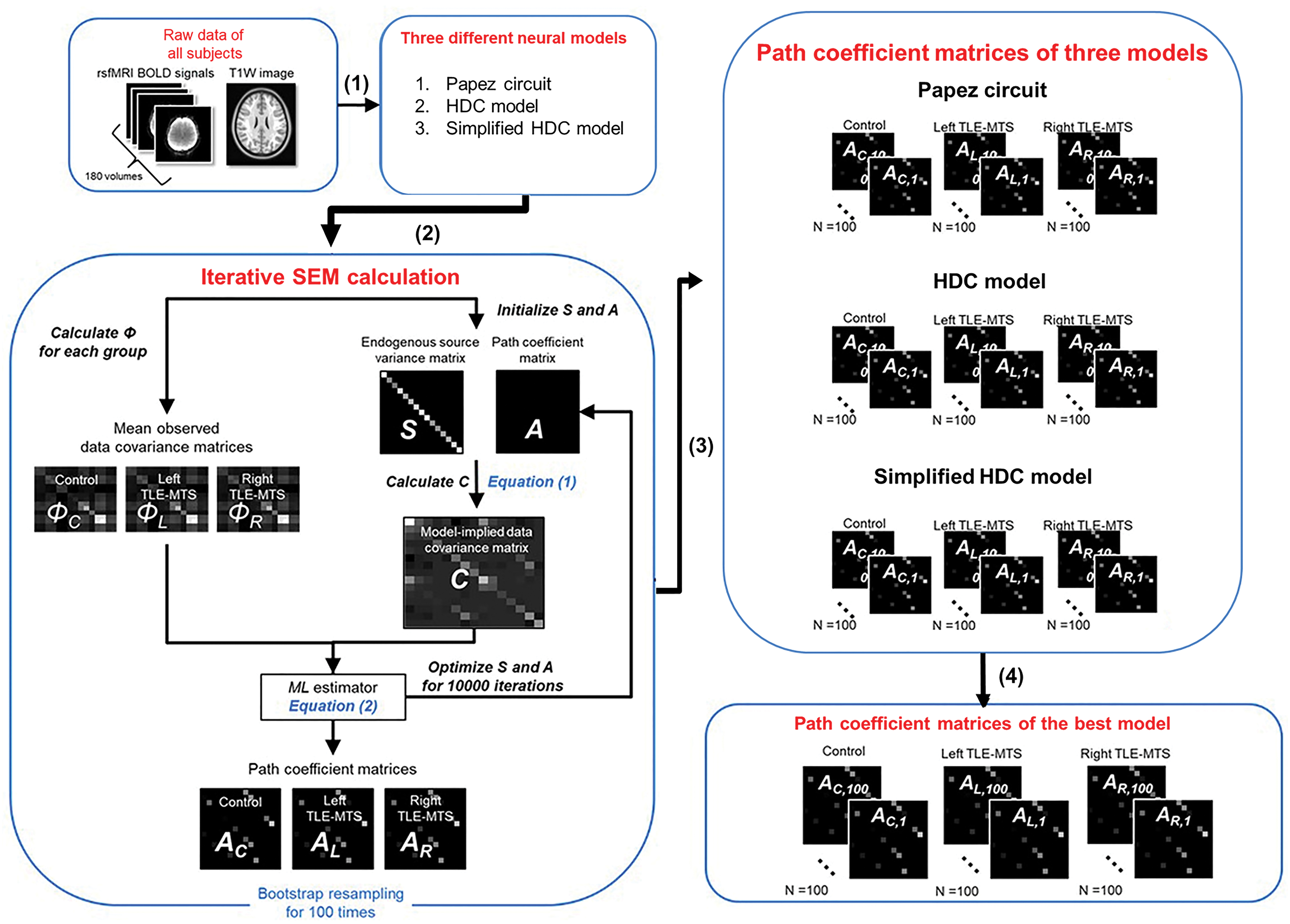
The procedures of SEM analysis. The overall procedure includes (1) data preprocessing, (2) path coefficient estimation using the SEM calculation with the ML optimization in three different neural models (or anatomically informed models), and (3) iterative SEM calculations. For each group, we used bootstrapping to randomly select participants with replacement for 100 iterations to estimate 100 path coefficients for each path. (4) Finally, we used the Akaike information criterion and Bayesian information criterion to select the best-fitted model. ML, maximum likelihood; MTS, mesial temporal sclerosis; SEM, structural equation modeling; T1W, T1-weighted imaging; TLE, temporal lobe epilepsy. Color images are available online.

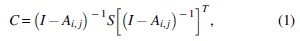
where A is the path coefficient matrix to be estimated, and the ith row and jth column of the matrix A and A_i,j represent the directional information flow from ROI_j to ROI_i. The .^T denotes the transposition of the matrix. S is the endogenous source variance matrix among the ROIs of a predefined brain network model. I is the identity matrix. To obtain the endogenous source variance matrix S, we assumed that the intrinsic variance of each ROI was 50% of the variance of rsfMRI BOLD signals and adopted it as a starting value (Lin et al., 2009).

We set the starting values of path coefficients to zero for initializing iterative calculation of the path coefficient matrix A. Given S and A, we ran model estimations for 10,000 iterations to estimate the model-implied data covariance matrix C. We adopted the maximum likelihood (ML) estimator to iteratively minimize the following cost function F_ML to estimate path coefficients (McArdle and McDonald, 1984):

where det(.) represents the determinant of a matrix, tr(.) represents the trace of a matrix, and p is the number of ROIs. Equation (2) indicated that the closer C was to Φ, the smaller F_ML was. The scale of the path coefficient, which represents the strength of iEC, can be interpreted as the amount of expected rsfMRI BOLD signal change at the destination ROI in response to one unit increase of the predicted rsfMRI BOLD signal change at the source ROI.

The three mean observed data covariance matrices were then used to respectively estimate path coefficients for the healthy controls, patients with left MTS, and patients with right MTS. For each group, we used bootstrapping to randomly select the participants with replacement (Efron and Tibshirani, 1993) for 100 iterations to estimate 100 path coefficients for each path. The one-sample t test was used to determine the statistical significance of a path. The Benjamini–Hochberg method was used to correct for multiple tests in each group.

The χ ² test was performed to evaluate the goodness of model fit for the three study groups. However, this test might not be reliable enough when the sample size is small (Bentler and Bonett, 1980), even though we adopted bootstrap resampling to increase the sample size to n = 100 in each group. Thus, we additionally calculated the root mean square error of approximation (RMSEA) to access the performance on model fit in each group (Hu and Bentler, 1998; James et al., 2009). The grand averaged RMSEA value with cutoff threshold (good fit: <0.05) over 100 iterative SEM calculations indicates good model fit (James et al., 2009; Rosseel, 2012). Next, for model selection, we introduced two comparative fit indices to quantitatively compare the goodness of model fit to rsfMRI BOLD signals in healthy controls, namely the Akaike information criterion (AIC) (Akaike, 1974) and the Bayesian information criterion (BIC) (Schwarz, 1978). Note that both fit indices are applicable while performing ML-based SEM analysis (Rosseel, 2012). Because of SEM for model fit with 100 iterations, each model fitting thereby produced 100 AIC and 100 BIC scores, respectively. Numerically, the candidate neural model with the lowest AIC and BIC values in healthy controls was selected as the best-fitted model (Huang, 2017; James et al., 2009; Rosseel, 2012), as iEC in healthy controls was considered as the standard to compared with the iEC in patients. The details of AIC, BIC, and RMSEA calculations are described in the Supplementary Data.

Statistical analyses

All statistical analyses were conducted using SPSS, Version 20 (IBM). We performed the Kruskal–Wallis test to compare the path coefficients of all paths in the best-fitted model between the healthy controls and patients with left or right MTS. The Mann–Whitney U test was performed as a post hoc test. The Benjamini–Hochberg method was employed to correct multiple comparisons.

Bootstrap resampling in ML-based SEM was adopted to gain the feasibility and robustness of obtaining the model fit statistic (i.e., an adjusted model test statistic p-value) and of estimating the path coefficients for each group (Yung and Bentler, 1996). Although this helped us assess the difference in iEC among the three study groups, it was not applicable to correlation analysis. Thus, to understand the relationship between aberrant iEC and seizure frequency in patients with unilateral MTS, we performed SEM calculations for path coefficients based on the observed covariance matrix of each patient. The path coefficients of the paths that showed a significant difference in the three-group comparison were used to correlate with seizure frequency. We performed the multivariate linear regression analysis to understand the relationship between the shared iEC alterations and seizure frequency in the patients with left and right MTS. The factors of age and gender were also included into this analysis. The same linear regression analysis was employed to search other potential relationships of the unique iEC alterations with seizure frequency in patients with left MTS and in patients with right MTS.

Results

Performance of model fitting

Overall, rsfMRI BOLD signals fitted all the proposed models for three study groups, namely the Papez circuit, HDC model, and simplified HDC model. In the χ ² test, lower χ ² value implied better model fitting and p > 0.99 indicated that the null-hypothesis H₀ was not rejected (Table 2; H₀: rsfMRI data fit the proposed model). The grand averaged RMSEA values of the three anatomically informed models in each group were small than 0.05, indicating good model fit (Table 2). Numerically, the simplified HDC model with the lowest mean AIC and BIC values had the best performance on model fitting among the three models (Table 3 and Supplementary Fig. S2) (Huang, 2017; James et al., 2009; Rosseel, 2012). To further confirm this result, we performed one-way analysis of variance to compare AIC and BIC among the three anatomically informed models. The Tukey–Kramer method was then used to assess the differences in AIC or BIC between the two models as a post hoc test. The post hoc tests revealed that the simplified HDC model with the lowest mean AIC and BIC values had the best performance on model fitting among the three models (Table 3). The simplified HDC model was thereby selected to conduct the following statistical analyses.

Table 2.

The Overall Performance of the Model Fitting Based on Three Different Anatomically Informed Models

Model name	Left MTS					Right MTS					Healthy controls
	χ² test			RMSEA	N.S. path #/total path #	χ² test			RMSEA	N.S. path #/total path #	χ² test			RMSEA	N.S. path #/total path #
	χ²	df	p	RMSEA	N.S. path #/total path #	χ²	df	p	RMSEA	N.S. path #/total path #	χ²	df	p	RMSEA	N.S. path #/total path #
Papez circuit	83.88	904	>0.99	0.0059	5/20	92.25	1036	>0.99	0.0051	3/20	259.88	2422	>0.99	0.0031	4/20
HDC model	88.49	1022	>0.99	0.0059	7/34	88.25	890	>0.99	0.0050	3/34	234.78	2408	>0.99	0.0029	8/34
Simplified HDC model	81.73	744	>0.99	0.0067	3/26	95.56	854	>0.99	0.0057	1/26	259.72	2009	>0.99	0.0034	3/26

In the χ ² test, the null-hypothesis H₀ is that resting-state functional magnetic resonance imaging data fit the proposed model, and p > 0.99 indicates that H₀ is not rejected by the χ ² test. The grand averaged RMSEA with a cutoff threshold of <0.05 indicates a good model fit. N.S. path assessed by one-sample t test indicates that its path coefficient is not significantly different from zero. “#” indicates the number of paths.

df, bootstrapped degree of freedom; HDC, hippocampal–diencephalic–cingulate; N.S., nonsignificant; RMSEA, root mean square error of approximation.

Table 3.

The Comparisons of Akaike Information Criterion and Bayesian Information Criterion Values Derived from Bootstrapped Structural Equation Modeling Analysis Among Three Different Anatomically Informed Models in Healthy Controls

Index	Model name	Mean	SD	F-value	p-Value	Post hoc analysis	p-Value
AIC	Papez circuit	331.86	39.67	—	—	Vs. HDC model	0.5557
	HDC model	336.74	29.32	—	—	Vs. Simplified HDC	0.0003
	Simplified HDC	318.11	34.19	—	—	Vs. Papez circuit	0.0107
				8.38	0.0003
BIC	Papez circuit	364.08	39.67	—	—	Vs. HDC model	≈0
	HDC model	391.51	29.32	—	—	Vs. Simplified HDC	≈0
	Simplified HDC	359.99	36.10	—	—	Vs. Papez circuit	0.6224
				26.38	≈ 0

AIC, Akaike information criterion; BIC, Bayesian information criterion; SD, standard deviation.

Path coefficients of the simplified HDC network

Path coefficients for 26 paths represent the strengths of iEC within the simplified HDC model. In healthy controls (Fig. 3, upper row), most paths were significant as assessed by the one-sample t test (Benjamini–Hochberg-corrected p < 0.05, the details are described in Supplementary Table S2), except for the paths left PCG→left ATN (p = 0.781), left ACG→left PCG (p = 0.217), right PCG→right ATN (p = 0.718), and right ACG→right PCG (p = 0.147). In patients with left MTS (Fig. 3, middle row), most paths were significant (Benjamini–Hochberg-corrected p < 0.05, the details are described in Supplementary Table S2), except for the paths left HP→left ATN (p = 0.277), MB→left ATN (p = 0.189), right PCG→right ATN (p = 0.666), and left PHG→right PHG (p = 0.129). In patients with right MTS (Fig. 3, lower row), most paths were significant (Benjamini–Hochberg-corrected p < 0.05, the details are described in Supplementary Table S2), except for the paths left PCG→left ATN (p = 0.106).

FIG. 3.

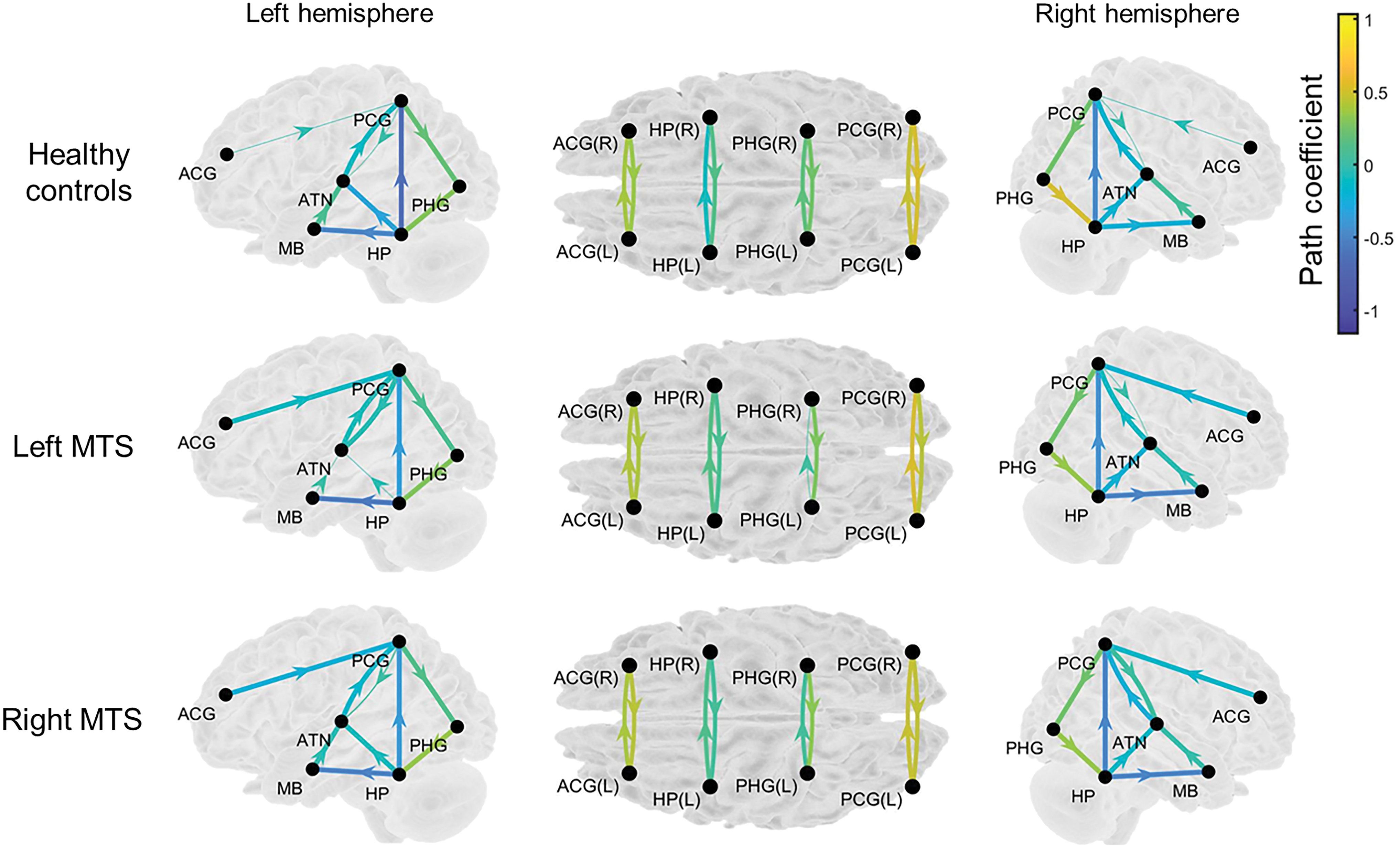
Path coefficients on the paths represent the strength of iEC within the simplified HDC model in the three study groups. The thicker arrows denote the significant paths assessed by the one-sample t test (Benjamini–Hochberg-corrected p < 0.05), whereas the thinner arrows indicate nonsignificant paths (Benjamini–Hochberg-corrected p < 0.05). The arrow with warmer color indicates the path with stronger iEC, and the arrow with cooler color indicates the path with weaker iEC. The exact uncorrected p-values are listed in Supplementary Table S2. iEC, intrinsic effective connectivity. Color images are available online.

Group comparison of path coefficients

Among the three groups, 10 paths, that is, left PCG→left PHG (F = 24.514, p ≈ 0), left HP→left PCG (F = 11.15, p = 2.1 × 10⁻⁵), left HP→left ATN (F = 12.17, p = 8 × 10⁻⁶), MB→left ATN (F = 57.603, p ≈ 0), left ACG→left PCG (F = 6.587, p = 0.002), right PHG→right HP (F = 25.041, p ≈ 0), right HP→MB (F = 12.438, p = 6 × 10⁻⁶), MB→right ATN (F = 36.679, p ≈ 0), left HP→right HP (F = 19.735, p ≈ 0), and right PCG→left PCG (F = 4.886, p = 0.008), showed significant differences in iEC. After the Benjamini–Hochberg multiple comparison correction (corrected p < 0.05), a path of right PCG→left PCG showed a slight difference in path coefficients. Figure 4 shows the results of post hoc analysis. Table 4 further summarizes the results of between-group comparisons. Compared with the healthy controls, the two patient groups showed shared iEC alterations on five paths with decreased iEC (left PCG→left PHG, MB→left ATN, right PHG→right HP, right HP→MB, and MB→right ATN) and three paths with increased iEC (left HP→left PCG, left HP→left ATN, and left HP→right HP). The findings displayed the common characteristics of iEC alterations of the simplified HDC model in TLE with left and right MTS. In addition to the shared alterations, patients with right MTS exhibited distinct alterations on left ACG→left PCG with decreased iEC.

FIG. 4.

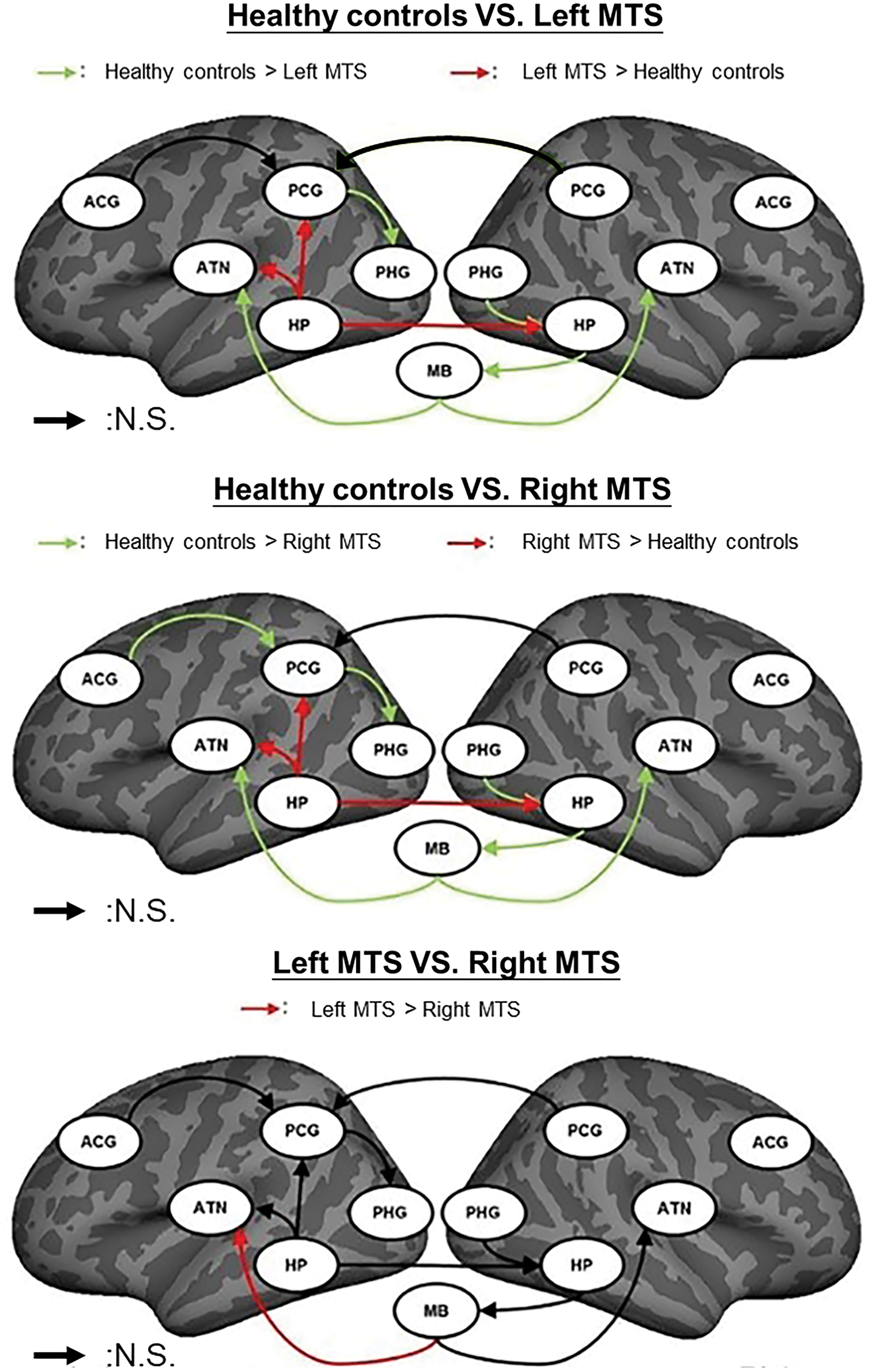
Post hoc between-group comparison results of the 10 paths in the simplified HDC model using the Mann–Whitney U test with Benjamini–Hochberg correction. The green and red arrows in the top and middle panels, respectively, indicate the paths with decreased and increased path coefficients in patients with TLE-MTS compared with healthy controls (Benjamini–Hochberg-corrected p < 0.05). The red arrow in the bottom panel indicates the paths with decreased path coefficients in patients with right TLE-MTS compared with patients with left TLE-MTS (Benjamini–Hochberg-corrected p < 0.05). The black arrow indicates the paths with insignificant differences in path coefficients between groups. N.S., nonsignificant. Color images are available online.

Table 4.

Summary of the Post Hoc Between-Group Comparison Results of the Nine Paths in the Simplified Hippocampal–Diencephalic–Cingulate Model

Paths		Left MTS vs. HC	Right MTS vs. HC	Left MTS vs. right MTS	Shared iEC alterations (left and right MTS vs. HC)	Distinct iEC alterations (left MTS vs. HC)	Distinct iEC alterations (right MTS vs. HC)
From	To	Left MTS vs. HC	Right MTS vs. HC	Left MTS vs. right MTS	Shared iEC alterations (left and right MTS vs. HC)	Distinct iEC alterations (left MTS vs. HC)	Distinct iEC alterations (right MTS vs. HC)
PCG (L)	PHG (L)	↓	↓	N.S.	↓	—	—
HP (L)	PCG (L)	↑	↑	N.S.	↑	—	—
HP (L)	ATN (L)	↑	↑	N.S.	↑	—	—
MB	ATN (L)	↓	↓	↑	↓	—	—
ACG (L)	PCG (L)	N.S.	↓	N.S.	—	—	↓
PHG (R)	HP (R)	↓	↓	N.S.	↓	—	—
HP (R)	MB	↓	↓	N.S.	↓	—	—
MB	ATN (R)	↓	↓	N.S.	↓	—	—
HP (L)	HP (R)	↑	↑	N.S	↑	—	—
PCG (R)	PCG (L)	↓^*	N.S.	N.S.	—	↓	—

↑ indicates increased iEC on the path of the former group compared with the latter group (Benjamini–Hochberg-corrected p < 0.05). ↓ indicates decreased iEC on the path of the former group compared with the latter group (Benjamini–Hochberg-corrected p < 0.05). ↓^* indicates a tendency of decreased iEC (Benjamini–Hochberg-corrected 0.05 < p < 0.1).

ACG, anterior cingulate gyrus; ATN, anterior thalamic nuclei; iEC, intrinsic effective connectivity; HC, healthy controls; L, left; MB, mammillary body; PCG, posterior cingulate gyrus; PHG, parahippocampal gyrus; R, right.

Associations between aberrant iEC and seizure frequency

In patients with unilateral MTS, we identified a significant linear relationship between aberrant iEC and seizure frequency (Table 5, adjusted-R ² = 0.350, p = 0.037), where the path coefficients on MB→left ATN (standardized β-value = 0.580, p = 0.013) and right HP→MB (standardized β-value = 0.541, p = 0.045) were positively correlated with seizure frequency, and path coefficients on path coefficients on right and path coefficients on MB→right ATN were negatively correlated with seizure frequency (standardized β-value = −0.711, p = 0.006). However, when considering left MTS or right MTS groups alone, we failed to detect any significant relationship between path coefficients and seizure frequency.

Table 5.

A Linear Relationship Between Path Coefficients and Seizure Frequency in the Two Patient Groups Revealed by the Stepwise Linear Regression Analysis

Multivariate linear regression model (n = 30)
	β-value	Standardized β-value	t-Value	p-Value	R²	Adjusted-R ²	F-value	p-Value
Path coefficients					0.574	0.350	2.561	0.037^*
PCG(L)→PHG(L)	4.493	0.252	1.266	0.221
HP(L)→PCG(L)	1.054	0.272	1.503	0.149
HP(L)→ATN(L)	1.135	0.238	1.274	0.218
MB→ATN(L)	9.912	0.580	2.726	0.013^*
PHG(R)→HP(R)	1.233	0.175	0.957	0.350
HP(R)→MB	2.056	0.541	2.147	0.045^*
MB→ATN(R)	−7.642	−0.711	−3.072	0.006^**
HP(L)→HP(R)	−1.743	−0.226	−1.312	0.205
Other variables
Age	0.076	0.305	1.594	0.127
Gender	1.403	0.317	1.735	0.099

p < 0.05.

p < 0.01.

L, left; R, right.

Discussion

To the best of our knowledge, the present study is the first to estimate iEC on the interconnected paths within the simplified HDC model using iterative SEM calculations, as well as to characterize shared and distinct iEC alterations in TLE patients with left and right MTS. By performing the linear regression analysis, the decreased iEC on the three parallel paths (MB→left ATN, MB→right ATN, and right HP→MB) emerges to be associated with seizure frequency in both patient groups. The findings indicate that functional abnormalities in the MB-associated connections represent the common neurophysiology of seizure recurrence.

The simplified HDC model is an appropriate neural model to estimate iEC

The χ ² test and RMSEA demonstrated that rsfMRI BOLD signals showed good performance of model fitting to the Papez circuit, HDC model, and simplified HDC model. The between-model comparisons of AIC and BIC scores indicated that the simplified HDC network was the most appropriate model to estimate iEC because the directionality of its paths was in agreement with the findings of previous neurophysiological studies (Bubb et al., 2017; Shah et al., 2012). iEC on the few nonsignificant paths assessed by the one-sample t test might be attributed to the high heterogeneity of variance of spontaneous rsfMRI data. Increasing the sample size of rsfMRI data for each study group might help improve SEM analysis to estimate iEC (Bentler and Bonett, 1980).

Relationships between aberrant iEC and seizure frequency in unilateral MTS

All the patients had opposing relationships between aberrant iEC and seizure frequency (Table 5), implying an asymmetry of aberrant iEC for the left and right mammillothalamic connections. Patients with frequent seizures had stronger directional information flows from the MB toward the left ATN, but weaker directional information flows from the MB toward the right ATN. Few fMRI studies have reported asymmetry in abnormal directional information flows between the MB and bilateral ATN in TLE with MTS. However, a preclinical study using electrical stimulation reported that left ATN stimulation successfully reduced the occurrence of seizure activity in rats with pilocarpine-induced epilepsy, whereas right ATN stimulation had little effect on seizure suppression (Jou et al., 2013). This suggests that left and right ATN have different tolerance thresholds to modulate epileptic seizures. The left ATN may be more sensitive to seizure intervention than the right ATN. In neuroanatomy, the mammillothalamic tract is the axonal substrate of a path on MB→ATN (Shibata, 1992). Recently, the ATN, MB, and mammillothalamic tract have been implicated in seizure propagation and generation (Balak et al., 2018; Möttönen et al., 2015). Despite there being no definite physiological mechanisms to explain why the left and right ATN stimulations produced distinct therapeutic outcomes and that the MB exerted different strengths of iEC to the left and right ATN, our findings of opposite correlations with seizure frequency may shed light on the finding of Jou et al. (2013).

Clinical relevance of the shared iEC alterations associated with seizure frequency

The relationship between decreased iEC on the bilateral mammillothalamic paths and seizure frequency characterized by our study could be valuable toward the pretreatment evaluation of unilateral MTS. The findings imply that therapy targeting the mammillothalamic tracts could be helpful for patients with drug-resistant TLE with unilateral MTS. A deep brain stimulation (DBS) study has proved the effectiveness of targeted therapy on the mammillothalamic tracts, resulting in seizure reduction and memory function improvement in patients with epilepsy (Balak et al., 2018). Future work is warranted to predict outcomes of memory performance and therapeutic efficacy following medical treatment on the basis of iEC on the bilateral mammillothalamic paths.

Moreover, Velasco et al. (2007) indicated that TLE patients with MTS had little improvements in seizure control compared with TLE patients without MTS after a treatment of electrical stimulation on the ipsilateral HP. It implies that, in TLE with MTS, the neural correlates of seizure occurrence might not be restricted to seizure onset zones of the HP, and they might involve more neural pathways beyond the mesial temporal region, such as the major hippocampal efferent projections of the fornix (Koubeissi et al., 2013) and mammillothalamic tracts. In fact, the fornix is the axonal substrate of the connection right HP→MB that we found to be in relation to seizure frequency. A review article also supports similar ideas that DBS applied to a specific neural circuit beyond the seizure onset zone is effective to suppress seizure occurrence (Zangiabadi et al., 2019).

The most TLE studies using different iEC analyses investigated causal influences only in the restricted brain regions, such as the interhemispheric hippocampal connections (Morgan et al., 2011) and the ipsilateral mesial temporal region (HP, PHG, and amygdala) (Park et al., 2018). It might restrict them from exploring other extratemporal pathways with iEC alterations that may be related to seizure recurrence. By contrast, the present study employed a well-described neural circuit to provide functional evidence of the occurrence rates of seizure, suggesting a potential imaging marker to predict seizure recurrence in patients with unilateral MTS.

Aberrant iEC in left and right MTS

We found minimal differences in iEC alterations between the left and right MTS groups (Fig. 4). Given that aberrant iEC was not restricted to the ipsilateral hemisphere, it represented a lack of lateralized iEC alterations in the two patient groups. The laterization of structural and functional changes ipsilateral to seizure onset in patients with unilateral MTS has been reported. However, growing evidence suggests that it is not always the case. Recent studies using rsfMRI and magnetoencephalography (MEG) indicated that the widespread decreases in functional connectivity could be observed in both the ipsilateral and contralateral hemispheres of patients with TLE with focal seizure (Englot et al., 2015; Maccotta et al., 2013). In particular, Englot et al. (2015) used resting-state MEG analysis and demonstrated the similar brain topological patterns of abnormal functional connectivity across the two hemispheres in left and right TLE.

In addition, an early study applying Granger causality analysis had reported that in patients with left and right mesial TLE, the left HP exerted more directional information flow to the right HP compared with the directional information flow from the right HP to the left HP (Morgan et al., 2011). This observation partially supports our findings that both MTS groups exhibited increased iEC from the left HP to other brain regions. Although the exact neurophysiology is unclear as to why greater iEC from the left HP was observed, an rsfMRI study also showed increased functional connectivity at the typical seizure onset regions in patients with TLE (Maccotta et al., 2013), thus implying an association between abnormal BOLD signals and seizure activity.

Moreover, Englot et al. (2016) reviewed past neuroimaging studies and further suggested a plausible mechanistic underpinning to describe how the long-term ictal effects of partial seizures lead to the global functional abnormalities. In patients with focal awareness seizure, seizure activity only occurs in the local mesial temporal lobe. When seizure activity propagates to brain regions beyond the ipsilateral mesial temporal lobe, it can lead to aberrant activities in the contralateral mesial temporal lobe and brain deactivations in the bilateral neocortices and result in the occurrence of focal impaired awareness seizure (FIAS). If seizure activity travels over the whole cortical regions, it can lead to the focal to bilateral tonic–clonic seizure. If we hypothesize that the increases and decreases in iEC respectively relate to seizure activity and brain deactivation, then our findings could be explained by the above mechanism of FIAS proposed by Englot et al. (2016). Coincidentally, the major seizure type in our two patient groups was FIAS (N, FIAS/other types = 25/5, Table 1), and it thereby supports the lack of lateralized iEC alterations.

In addition, we realized that studying iEC within the limbic regions was challenging. In fact, in the ROI-based approach to functional connectivity, the voxel number of an ROI was suggested to be in the range of tens to hundreds of voxels (Stanley et al., 2013). Some limbic ROIs (e.g., MB and ATN) with smaller volume comprising only a few voxels might be easily affected by head motion. Spatial smoothing could be helpful to reduce such impact but would potentially induce the partial volume effect as well. Alternatively, spatial normalization to the MNI template with spatial resolution of 1 × 1 × 1 mm³ would increase the voxel number of the ROIs of MB and ATN in rsfMRI data. In this study, the spatial resolution of raw rsfMRI data was 4 × 4 × 3 mm³ and much larger than that of 1 × 1 × 1 mm³ in the MNI template. Hence, the excessive interpolation in the spatial normalization could severely distort rsfMRI data. A better solution is to acquire rsfMRI data with ultrahigh spatial resolution using the multiband accelerated technique. Recently, Tanaka et al. (2020) performed this accelerated acquisition scheme (multiband factor = 4) with spatial resolution of 1.25 × 1.25 × 1.25 mm³ to measure rsfMRI BOLD signals in the MB. However, as the multiband rsfMRI sequence in our hospital was a work in progress sequence provided by the vendor, it was not available to the present clinical study. The impact of head motion might lead to lower temporal signal-to-noise ratio (tSNR) of BOLD signals in those smaller ROIs. The results showed that tSNR among all ROIs with different sizes did not show significant difference in each study group (Supplementary Fig. S1), and the different ROI volumes would not significantly affect our analysis.

Limitations

First, we constrained the directionality of each path on the basis of the prior knowledge of the simplified HDC model to construct the implied data covariance matrix. This approach prevented us from changing the directionality of the path in the SEM analysis. The inference of directionality within the simplified HDC model should be verified by other invasive techniques, such as corticocortical evoked potential (Enatsu et al., 2015). Second, the pathological evidence of MTS is not available because all patients in this study did not undergo surgical resection of the brain. Visual inspection of MTS on the basis of structural MRI images may not be sufficient to clearly identify hippocampal sclerosis. Quantitative structural MRI analyses have been suggested to be more sensitive to detect hippocampal sclerosis than visual inspection (Bernasconi, 2006). Therefore, we assessed hippocampal atrophy by comparing the hippocampal volume between the study groups to confirm the MTS side for our patients. Third, we realized that seizure frequency estimated by self-report and interviews of patients and their family members might not be precise enough. It can be improved by implanting the depth electrodes on the seizure focus to monitor the long-term intracranial EEG (Parvizi and Kastner, 2018). However, such invasive monitoring is not available in this study. Nevertheless, by following the Engel classification (Engel, 1993), Park et al. (2018) had also reported that the intratemporal iEC was influenced by seizure frequency, which was also obtained from the information of seizure diaries. Finally, our small sample size was due to the strict criteria for screening for pure unilateral MTS patients. To address this problem, the present study adopted the bootstrap resampling method to increase the sample size of each patient group. Nevertheless, our findings should be verified by a larger cohort study.

Conclusions

The present study has verified that the simplified HDC model was a more appropriate model than the Papez circuit to estimate iEC in unilateral MTS. Within the simplified HDC model, associations between iEC alterations and seizure frequency have been found. The knowledge could provide valuable insights into aberrant directional information flows in epilepsy, and their neurophysiological significance relevant to seizure recurrence. Our findings could facilitate the discovery of potential epilepsy pathways and the development of novel targeted therapies for TLE with unilateral MTS.

Footnotes

Authors' Contributions

Y.-C.S. collected all data, performed the data and statistical analyses, and wrote the article. F.-H.L. implemented the analytic method. H.-H.L. helped data collection, designed, and supervised the study. W.-Y.I.T. supervised the study and wrote the article.

Acknowledgments

We thank Aeden Kuek Zi Cheng who is a research assistant in the Department of Diagnostic Radiology, Singapore General Hospital, for editing the article, and Wallace Academic Editing for proofreading the article.

Author Disclosure Statement

No competing financial interests exist.

Funding Information

The study was funded in part by Taiwan Ministry of Science and Technology for supporting (grant number: MOST106-2314-B-002-203).

Supplementary Material

Supplementary Data

Supplementary Figure S1

Supplementary Figure S2

Supplementary Table S1

Supplementary Table S2

References

Aggleton

, Saunders

, Wright

, et al. 2014. The origin of projections from the posterior cingulate and retrosplenial cortices to the anterior, medial dorsal and laterodorsal thalamic nuclei of macaque monkeys. Eur J Neurosci, 39:107–123.

Aggleton

, Wright

, Rosene

, et al. 2015. Complementary patterns of direct amygdala and hippocampal projections to the macaque prefrontal cortex. Cereb Cortex, 25:4351–4373.

Akaike

. 1974. A new look at the statistical model identification. IEEE Trans Automat Contr, 19:716–723.

Ashburner

. 2007. A fast diffeomorphic image registration algorithm. Neuroimage, 38:95–113.

Balak

, Balkuv

, Karadag

, et al. 2018. Mammillothalamic and mammillotegmental tracts as new targets for dementia and epilepsy treatment. World Neurosurg, 110:133–144.

Bentler

, Bonett

. 1980. Significance tests and goodness of fit in the analysis of covariance structures. Psychol Bull, 88:588–606.

Bernasconi

. 2006. Magnetic resonance imaging in intractable epilepsy: focus on structural image analysis. Adv Neurol, 97:273–278.

Bernhardt

, Worsley

, Kim

, et al. 2009. Longitudinal and cross-sectional analysis of atrophy in pharmacoresistant temporal lobe epilepsy. Neurology, 72:1747–1754.

Bharath

, Sinha

, Panda

, et al. 2015. Seizure frequency can alter brain connectivity: evidence from resting-state fMRI. AJNR Am J Neuroradiol, 36:1890–1898.

10.

Bubb

, Kinnavane

, Aggleton

. 2017. Hippocampal—diencephalic—cingulate networks for memory and emotion: an anatomical guide. Brain Neurosci Adv, 1:2398212817723443.

11.

Caciagli

, Bernasconi

, Wiebe

, et al. 2017. A meta-analysis on progressive atrophy in intractable temporal lobe epilepsy: time is brain?. Neurology, 89:506–516.

12.

Dillingham

, Erichsen

, O'Mara

, et al. 2015. Fornical and nonfornical projections from the rat hippocampal formation to the anterior thalamic nuclei. Hippocampus, 25:977–992.

13.

Efron

, Tibshirani

. 1993. An Introduction to the Bootstrap. New York, NY; London: Chapman & Hall.

14.

Enatsu

, Gonzalez-Martinez

, Bulacio

, et al. 2015. Connections of the limbic network: a corticocortical evoked potentials study. Cortex, 62:20–33.

15.

Engel

Jr.

1993. Update on surgical treatment of the epilepsies. Summary of the Second International Palm Desert Conference on the Surgical Treatment of the Epilepsies (1992). Neurology, 43:1612–1617.

16.

Englot

, Hinkley

, Kort

, et al. 2015. Global and regional functional connectivity maps of neural oscillations in focal epilepsy. Brain, 138(Pt 8):2249–2262.

17.

Englot

, Konrad

, Morgan

. 2016. Regional and global connectivity disturbances in focal epilepsy, related neurocognitive sequelae, and potential mechanistic underpinnings. Epilepsia, 57:1546–1557.

18.

Fisher

, Cross

, French

, et al. 2017. Operational classification of seizure types by the International League Against Epilepsy: position paper of the ILAE Commission for Classification and Terminology. Epilepsia, 58:522–530.

19.

Fox

, Snyder

, Vincent

, et al. 2005. The human brain is intrinsically organized into dynamic, anticorrelated functional networks. Proc Natl Acad Sci U S A, 102:9673–9678.

20.

Friston

, Kahan

, Biswal

, et al. 2014. A DCM for resting state fMRI. Neuroimage, 94:396–407.

21.

L-t

, Bentler

. 1998. Fit indices in covariance structure modeling: sensitivity to underparameterized model misspecification. Psychol Methods, 3:424–453.

22.

Huang

P-H

. 2017. Asymptotics of AIC, BIC, and RMSEA for model selection in structural equation modeling. Psychometrika, 82:407–426.

23.

Inman

, James

, Hamann

, et al. 2012. Altered resting-state effective connectivity of fronto-parietal motor control systems on the primary motor network following stroke. Neuroimage, 59:227–237.

24.

James

, Kelley

, Craddock

, et al. 2009. Exploratory structural equation modeling of resting-state fMRI: applicability of group models to individual subjects. Neuroimage, 45:778–787.

25.

, Zhang

, et al. 2013. Disrupted causal connectivity in mesial temporal lobe epilepsy. PLoS One, 8:e63183.

26.

Jou

, Kao

, Yi

, et al. 2013. Electrical stimulation of left anterior thalamic nucleus with high-frequency and low-intensity currents reduces the rate of pilocarpine-induced epilepsy in rats. Seizure, 22:221–229.

27.

Koubeissi

, Kahriman

, Syed

, et al. 2013. Low-frequency electrical stimulation of a fiber tract in temporal lobe epilepsy. Ann Neurol, 74:223–231.

28.

Krüger

, Kastrup

, Glover

. 2001. Neuroimaging at 1.5 T and 3.0 T: comparison of oxygenation-sensitive magnetic resonance imaging. Magn Reson Med, 45:595–604.

29.

Kwan

, Brodie

. 2000. Early identification of refractory epilepsy. N Engl J Med, 342:314–319.

30.

Lancaster

, Woldorff

, Parsons

, et al. 2000. Automated Talairach atlas labels for functional brain mapping. Hum Brain Mapp, 10:120–131.

31.

Laufs

, Lengler

, Hamandi

, et al. 2006. Linking generalized spike-and-wave discharges and resting state brain activity by using EEG/fMRI in a patient with absence seizures. Epilepsia, 47:444–448.

32.

Laxpati

, Kasoff

, Gross

. 2014. Deep brain stimulation for the treatment of epilepsy: circuits, targets, and trials. Neurotherapeutics, 11:508–526.

33.

Lee

, Arora

, Papademetris

, et al. 2014. Altered functional connectivity in seizure onset zones revealed by fMRI intrinsic connectivity. Neurology, 83:2269–2277.

34.

Lin

, Agnew

, Belliveau

, et al. 2009. Functional and effective connectivity of visuomotor control systems demonstrated using generalized partial least squares and structural equation modeling. Hum Brain Mapp, 30:2232–2251.

35.

Möttönen

, Katisko

, Haapasalo

, et al. 2015. Defining the anterior nucleus of the thalamus (ANT) as a deep brain stimulation target in refractory epilepsy: delineation using 3 T MRI and intraoperative microelectrode recording. Neuroimage Clin, 7:823–829.

36.

Maccotta

, He

, Snyder

, et al. 2013. Impaired and facilitated functional networks in temporal lobe epilepsy. Neuroimage Clin, 2:862–872.

37.

McArdle

, McDonald

. 1984. Some algebraic properties of the Reticular Action Model for moment structures. Br J Math Stat Psychol 37 (Pt 2):234–251.

38.

McIntosh

, Grady

, Ungerleider

, et al. 1994. Network analysis of cortical visual pathways mapped with PET. J Neurosci, 14:655–666.

39.

Morgan

, Rogers

, Sonmezturk

, et al. 2011. Cross hippocampal influence in mesial temporal lobe epilepsy measured with high temporal resolution functional magnetic resonance imaging. Epilepsia, 52:1741–1749.

40.

Papez

. 1937. A proposed mechanism of emotion. J Neuropsychiatry Clin Neurosci, 7:103–112.

41.

Park

, Choi

, Kim

, et al. 2018. Interactive effects of seizure frequency and lateralization on intratemporal effective connectivity in temporal lobe epilepsy. Epilepsia, 59:215–225.

42.

Parvizi

, Kastner

. 2018. Promises and limitations of human intracranial electroencephalography. Nat Neurosci, 21:474–483.

43.

Power

, Barnes

, Snyder

, et al. 2012. Spurious but systematic correlations in functional connectivity MRI networks arise from subject motion. Neuroimage, 59:2142–2154.

44.

Pressl

, Brandner

, Schaffelhofer

, et al. 2019. Resting state functional connectivity patterns associated with pharmacological treatment resistance in temporal lobe epilepsy. Epilepsy Res, 149:37–43.

45.

Rosseel

. 2012. lavaan: an R package for structural equation modeling. J Stat Softw, 48:36.

46.

Rowe

, Stephan

, Friston

, et al. 2002. Attention to action in Parkinson's disease: impaired effective connectivity among frontal cortical regions. Brain, 125(Pt 2):276–289.

47.

Schwarz

. 1978. Estimating the dimension of a model. Ann Stat, 6:461–464.

48.

Shah

, Jhawar

, Goel

. 2012. Analysis of the anatomy of the Papez circuit and adjoining limbic system by fiber dissection techniques. J Clin Neurosci, 19:289–298.

49.

Shibata

. 1992. Topographic organization of subcortical projections to the anterior thalamic nuclei in the rat. J Comp Neurol, 323:117–127.

50.

Stanley

, Moussa

, Paolini

, et al. 2013. Defining nodes in complex brain networks. Front Comput Neurosci, 7:169.

51.

Tanaka

, Osada

, Ogawa

, et al. 2020. Dissociable networks of the lateral/medial mammillary body in the human brain. Front Hum Neurosci, 14:228.

52.

Velasco

, Velasco

, et al. 2007. Electrical stimulation of the hippocampal epileptic foci for seizure control: a double-blind, long-term follow-up study. Epilepsia, 48:1895–1903.

53.

Wei

, Mao

, Cong

, et al. 2017. In vivo visualization of connections among revised Papez circuit hubs using full q-space diffusion spectrum imaging tractography. Neuroscience, 357:400–410.

54.

Wiebe

, Jette

. 2012. Pharmacoresistance and the role of surgery in difficult to treat epilepsy. Nat Rev Neurol, 8:669–677.

55.

Xiang

J-Z

, Brown

. 2004. Neuronal responses related to long-term recognition memory processes in prefrontal cortex. Neuron, 42:817–829.

56.

Yan

, Zang

. 2010. DPARSF: a MATLAB toolbox for “pipeline” data analysis of resting-state fMRI. Front Syst Neurosci, 4:13.

57.

Yung

, Bentler

. 1996. Bootstrapping techniques in analysis of mean and covariance structures. In: Marcoulides GA, Schumacker RE (eds.) Advanced Structural Equation Modeling Techniques. New Jersey: Erlbaum, pp. 195–226.

58.

Zangiabadi

, Ladino

, Sina

, et al. 2019. Deep brain stimulation and drug-resistant epilepsy: a review of the literature. Front Neurol, 10:601.

Supplementary Material

Please find the following supplemental material available below.

For Open Access articles published under a Creative Commons License, all supplemental material carries the same license as the article it is associated with.

For non-Open Access articles published, all supplemental material carries a non-exclusive license, and permission requests for re-use of supplemental material or any part of supplemental material shall be sent directly to the copyright owner as specified in the copyright notice associated with the article.

0.00 MB

0.02 MB

0.15 MB

0.01 MB