Tri-Clustering Dynamic Functional Network Connectivity Identifies Significant Schizophrenia Effects Across Multiple States in Distinct Subgroups of Individuals

Abstract

Background:

Brain imaging data collected from individuals are highly complex with unique variation; however, such variation is typically ignored in approaches that focus on group averages or even supervised prediction. State-of-the-art methods for analyzing dynamic functional network connectivity (dFNC) subdivide the entire time course into several (possibly overlapping) connectivity states (i.e., sliding window clusters). However, such an approach does not factor in the homogeneity of underlying data and may result in a less meaningful subgrouping of the data set.

Methods:

Dynamic-N-way tri-clustering (dNTiC) incorporates a homogeneity benchmark to approximate clusters that provide a more “apples-to-apples” comparison between groups within analogous subsets of time-space and subjects. dNTiC sorts the dFNC states by maximizing similarity across individuals and minimizing variance among the pairs of components within a state.

Results:

Resulting tri-clusters show significant differences between schizophrenia (SZ) and healthy control (HC) in distinct brain regions. Compared with HC subjects, SZ show hypoconnectivity (low positive) among subcortical, default mode, cognitive control, but hyperconnectivity (high positive) between sensory networks in most tri-clusters. In tri-cluster 3, HC subjects show significantly stronger connectivity among sensory networks and anticorrelation between subcortical and sensory networks than SZ. Results also provide a statistically significant difference in SZ and HC subject's reoccurrence time for two distinct dFNC states.

Conclusions:

Outcomes emphasize the utility of the proposed method for characterizing and leveraging variance within high-dimensional data to enhance the interpretability and sensitivity of measurements in studying a heterogeneous disorder such as SZ and unconstrained experimental conditions as resting functional magnetic resonance imaging.

Impact statement

The current methods for analyzing dynamic functional network connectivity (dFNC) run k-means on a collection of dFNC windows, and each window includes all the pairs of independent component analysis networks. As such, it depicts a short-time connectivity pattern of the entire brain, and the k-means clusters fixed-length signatures that have an extent throughout the neural system. Consequently, there is a chance of missing connectivity signatures that span across a smaller subset of pairs. Dynamic-N-way tri-clustering further sorts the dFNC states by maximizing similarity across individuals, minimizing variance among the pairs of components within a state, and reporting more complex and transient patterns.

Introduction

Heterogeneity in schizophrenia (SZ) represents a challenge for studying and diagnosing this disorder (Alnæs et al., 2019; Rahaman et al., 2020; Tsuang et al., 1990). A substantial amount of research effort has focused on identifying the causes of SZ, that would aid in improving diagnosis and treatments, yet we are still not close to the root cause of this mental illness (Du et al., 2020; Ferri et al., 2018; Lawrie and Abukmeil, 1998; Rashid et al., 2019). Studies often use structural magnetic resonance imaging (MRI), resting-state functional MRI (fMRI), and task-based fMRI to analyze a wide range of neurocognitive variables; for instance, brain network activation, subtyping, and neural components clustering (Allen et al., 2011; Calhoun et al., 2008; Rahaman et al., 2020). Resting-state fMRI is a widely used method for exploring neural activity—because it has the benefit of being both easy for patients to perform and potentially more sensitive to brain disorders (Damoiseaux et al., 2006; Franco et al., 2009; Shehzad et al., 2009; Zuo et al., 2010). Studies during rest fMRI have identified several temporally coherent networks that are putatively involved in functions such as vision, audition, and directing attention (Beckmann et al., 2005; Calhoun et al., 2001). More recent studies have exploited the dynamics and intrinsic fluctuations of connectivity (Arieli et al., 1996; Kucyi and Davis, 2014; Leonardi and Van De Ville, 2015; Makeig et al., 2004; Onton et al., 2006).

Dynamic functional network connectivity (dFNC) is a well-studied approach for analyzing the dynamics of the human brain. It provides time-varying correlation matrices typically computed using a sliding window (e.g., 44 sec in length) to estimate the connection among brain regions or independent components (ICs) of interest (Allen et al., 2011, 2014; Hindriks et al., 2016; Ioannides, 2007). In this study, each correlation is considered a transient functional association between functional networks (Ioannides, 2007). dFNC has also been appeared to be sensitive to various brain neurodegenerative diseases (Fu et al., 2018; Klugah-Brown et al., 2019; Ma et al., 2014; Vergara et al., 2018; Wang et al., 2020). The implementations vary across multiple aims of studying neural systems, including analyzing transition frequency, improving classification accuracy (Cetin et al., 2016; Rashid et al., 2016; Sakoglu et al., 2009), and capturing intermittent connectivity (Du et al., 2017). Moreover, dFNC provides crucial insights about the underlying dynamics in SZ, which might not be available in static investigations (Ma et al., 2014; Rashid et al., 2016). However, a typical sliding window plus clustering (SWC) analysis approach continuously models the system through a fixed set of connectivity patterns or states (Allen et al., 2011, 2014; Miller et al., 2016; Shakil et al., 2016). These approaches cluster the dFNC windows of a subject using k-means or some other clustering methods. It essentially assigns all the dFNC windows into some states but does not directly optimize their subject-wise consistency. Here, the window is a vector of “m” real values where each value represents the connectivity strength between a pair of brain components and “m” is the number of pairs available. This assumes each window carries information from all the pairs (connections); consequently, the approach explores patterns throughout the brain. In practice, connectivity signatures are more spatially constrained and often spread over a smaller subset of components (Miller et al., 2016), and different subsets showcase different types of connectivity patterns. As such, for the connectivity signatures that are more transient and have a comparatively lesser scope, that is, beyond a noncontiguous smaller subset of functional brain units, SWC fails to capture the patterns and reflect them in the clustering process. Consequently, it hinders our capability to investigate the brief and transient patterns of dFNC trajectories and their differences in distinct subject's group. In this study, we argued the necessity of further sorting the subset of subjects, pair of components, and time points enclosed within the dFNC states. So, our key hypothesis is that by focusing on a more homogeneous subset of the subject, connectivity pairs, and windows, we can increase sensitivity to brain disorder and associations with symptom measures. SWC considers all the pairs together and search for a connectivity pattern, assuming it spans throughout the brain. However, in practice, connectivity signatures often spread over a smaller subset of components (spatially constrained), and different subsets showcase different connectivity patterns. Hence, we need an approach that allows us to investigate the system more independently by looking at the relations within a subset of the brain regions. To localize the exploration and identify meaningful patterns, we propose to cluster all three dimensions (subjects, windows, and network pairs) of the data set together to extract more homogenous subgroups to provide a better comparison.

In three-dimensional (3D) data, observations are generally meaningfully correlated across various dimensions of the dynamic. As such, one-dimensional (1D) clustering is not likely to provide the most effective means of exploration. Although biclustering partially takes care of this challenge and is more effective, it does not include the third dimension (Rahaman et al., 2020). As dFNC is a 3D representation of the data, we might be missing significant group differences in the data by not clustering all three dimensions. Dynamic-N-way tri-clustering (dNTiC) simultaneously clusters three neural variables and return subgroups of entities with a maximized homogeneity across those given variables. Our approach, to our knowledge, represents the first attempt at exploring all three dimensions of dFNC and a robust method of tri-clustering multiple neural features. We perform more rigorous sorting on the subject within a state while keeping each of their windows highly correlated with the cluster centroid. dNTiC compacts the connectivity patterns by ignoring the heterogeneous connections and weakly correlated subjects; results show it still identifies more group differences than the 1D k-means approach, presumably because comparisons are more stable and meaningful (Allen et al., 2014). These tri-clusters report significant Patient (SZ)-healthy control (HC) group differences described in the results section. In an earlier study, the states were very similar for both SZ and HC groups; therefore, the differences are very subtle. In this study, we observe SZ < HC connectivity strength across Auditory (AUD), Visual (VIS), and Sensorimotor (SM) regions, and SZ > HC at subcortical (SC) in tri-clusters 3 and 5. In tri-cluster 1, we observe SZ > HC in AUD, VIS, and SM domains. The experiment on reoccurrence time reveals two subgroups showing a statistically significant difference between patient and control (tri-clusters 2 and 5). Overall, HC subjects show higher reoccurrence time than SZ except subgroup 2.

Data Collection and Preprocessing

In this study, we used resting-state fMRI data collected as part of the Functional Imaging Biomedical Informatics Research Networks project consisting of 163 HCs and 151 age- and gender-matched patients with SZ in a total of 314 subjects (Keator et al., 2016; Turner et al., 2013). The data set includes 117 males, 49 females; mean age of 36.9 from a healthy cohort, 114 males, 37 females; mean age of 37.8 from patients with SZ. More demographics of the samples are available in the earlier references and reported in Allen and associates (2014). The data acquisition and preprocessing follow a similar pipeline described in Damaraju and associates (2014) (Allen et al., 2014). Data quality control, head motion correction, and diagnosis are also described in this study's Supplementary Data. The collecting study ensured the informed consent of all participants before scanning. In brief, a blood oxygenation level-dependent fMRI scan was performed on 3T scanners across seven sites with patients and controls collected at all sites. Resting-state fMRI scans were acquired using the parameters FOV of 220 × 220 mm (64 × 64 matrix), TR = 2 sec, TE = 30 ms, FA = 770, 162 volumes, axial slices = 32, slice thickness = 4 mm, and skip = 1 mm. The scan was a closed eye resting-state fMRI acquisition. Image preprocessing was conducted using several toolboxes, namely AFNI, SPM, GIFT, and custom MATLAB scripts. First, rigid body motion correction was performed using SPM to correct for subject head motion and slice-timing correction for timing differences in slice acquisition. Then time series data are despiked to mitigate the outlier effect and warped to a Montreal Neurological Institute template and resampled to 3 mm³ isotropic voxels and followed by smoothing and variance normalization. The data smoothing is done to 6 mm full width at half maximum using AFNI's BlurToFWHM algorithm.

After preprocessing, we ran a group independent component analysis (Calhoun et al., 2001; Erhardt et al., 2011) on the functional data. We performed group independent component analysis (ICA) on the preprocessed data and identified 47 intrinsic connectivity networks (ICNs) from the decomposition of 100 components. Spatial maps and time courses for each subject were obtained using the spatiotemporal regression back reconstruction approach (Calhoun et al., 2001). Subject-wise spatial maps and time courses are then postprocessed as described in this article (Allen et al., 2014). The post-ICA processing for error control and corrections is described more elaborately in early mentioned studies. In this study, we discuss the steps concisely. The processing generates one sample t-test map for each spatial map across all subjects and threshold them to obtain regions of peak activation clusters for that component. Then we computed the mean power spectra of the corresponding time courses. Followed by that, we selected a set of components as ICNs if their peak activation clusters fell on gray matter and showed less overlap with known vascular, susceptibility, ventricular, and edge regions corresponding to head motion. Moreover, we ensured that the mean power spectra of the selected ICN time courses showed higher low-frequency spectral power. This selection procedure resulted in 47 ICNs out of the 100 ICs obtained. The cluster stability/quality (I _q) index for these ICNs over 20 ICASSO (a portmanteau of Independent Component Analysis [ICA] and least absolute shrinkage and selection operator [LASSO] for investigating the reliability of ICA estimates) runs was very high (I _q > 0.9) for all of the components, except an ICN that resembles the language network (I _q = 0.74). The subject-specific time course corresponding to the ICs selected were detrended, orthogonalized with respect to estimated subject motion parameters, and then despiked. The despiking procedure involved detecting spikes as determined by AFNI's 3dDespike algorithm and replacing spikes by values obtained from the third-order spline fit to neighboring clean portions of the data. The despiking process reduces the impact/bias of outliers on subsequent FNC measures. The dFNC between two ICA time courses was computed using a sliding window approach with a 22 TR (44 sec) window size in steps of 1 TR. The sliding window is a rectangular window of 22 time points convolved with Gaussian of sigma 3 TRs to obtain tapering along the edges (Allen et al., 2014). We computed covariance from regularized inverse covariance matrix (ICOV) (Smith et al., 2011; Varoquaux et al., 2010) using graphical Lasso framework (Friedman et al., 2008). Moreover, to ensure sparsity, we imposed an additional L1 norm constraint on the ICOV. We used a log-likelihood of unseen data of the subject in a cross-validation framework for optimizing regularization parameters. To ensure the positive semidefiniteness of the evaluated dynamic covariance matrices, we ensure their estimated eigenvalues are positive. Then we compute the dFNC values for each subject. Moreover, the covariance values are Fisher-Z transformed and residualized for age, gender, and sites.

Definitions

Definition 1: dFNC matrix

A dFNC matrix D is a symmetric matrix of n × n, where n is the number of components we consider, for example, 47. Each cell of the matrix represents the functional connectivity (FC) strength between two ICs.

Definition 2: dFNC window

A vector of size k where each value demonstrates a connection between two brain networks and k is the number of pairs of components or connections in the analysis. The transformation of the dFNC matrix to a 1D vector generates a dFNC window.

Definition 3: dFNC time series

A subject's dFNC time course, T = W₁, W_2, W_3, …, W_n is a sequential set of n real values, where W_i represents the correlation between two ICs of the brain for a certain period. W stands for the window.

Definition 4: dFNC state

dFNC state, S is a finite collection of homogenous dFNC windows from various subjects. Typically, the collection is evaluated by a clustering approach such as k-means.

Definition 5: sorted dFNC state

A sorted dFNC state is a subset of subjects, windows, and pairs of networks within a window after maximizing homogeneity across these dimensions.

Methods

Our methodology consists of three fundamental steps: (1) computing dFNC states, (2) sorting the states, and (3) exploring subsets of states, as shown in Figure 1. Figure 2 shows the different dimensions of our dFNC data set. Our method aims to cluster these dimensions simultaneously to generate tri-clusters. The proposed framework's input is the dFNC time course collected from patients with SZ and HC.

FIG. 1.

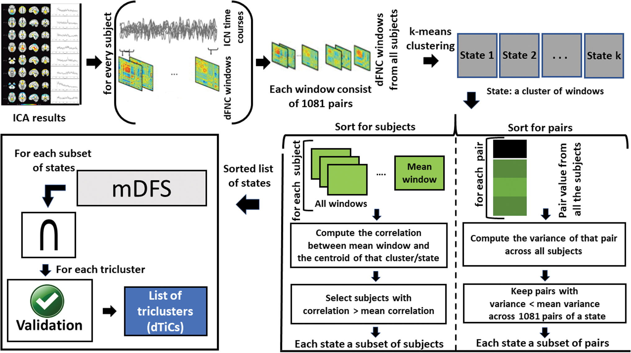
Our proposed tri-clustering framework. It consists of three basic subroutines: (1) clustering the windows from all the subjects into a certain number of clusters/states using standard k-means. (2) Sorting the states in two dimensions (subject and pair) for maximizing homogeneity across the attributes of a dFNC state. The step characterizes states as a subset of subjects and pairs. It downsizes the collection of windows (thus number of subjects) included in a state by removing weakly allied windows from the state. (3) Tri-clustering the sorted states by exploring all possible subsets of a given set of states using an mDFS technique enriched by early abandoning. mDFS, modified depth-first search. Color images are available online.

FIG. 2.

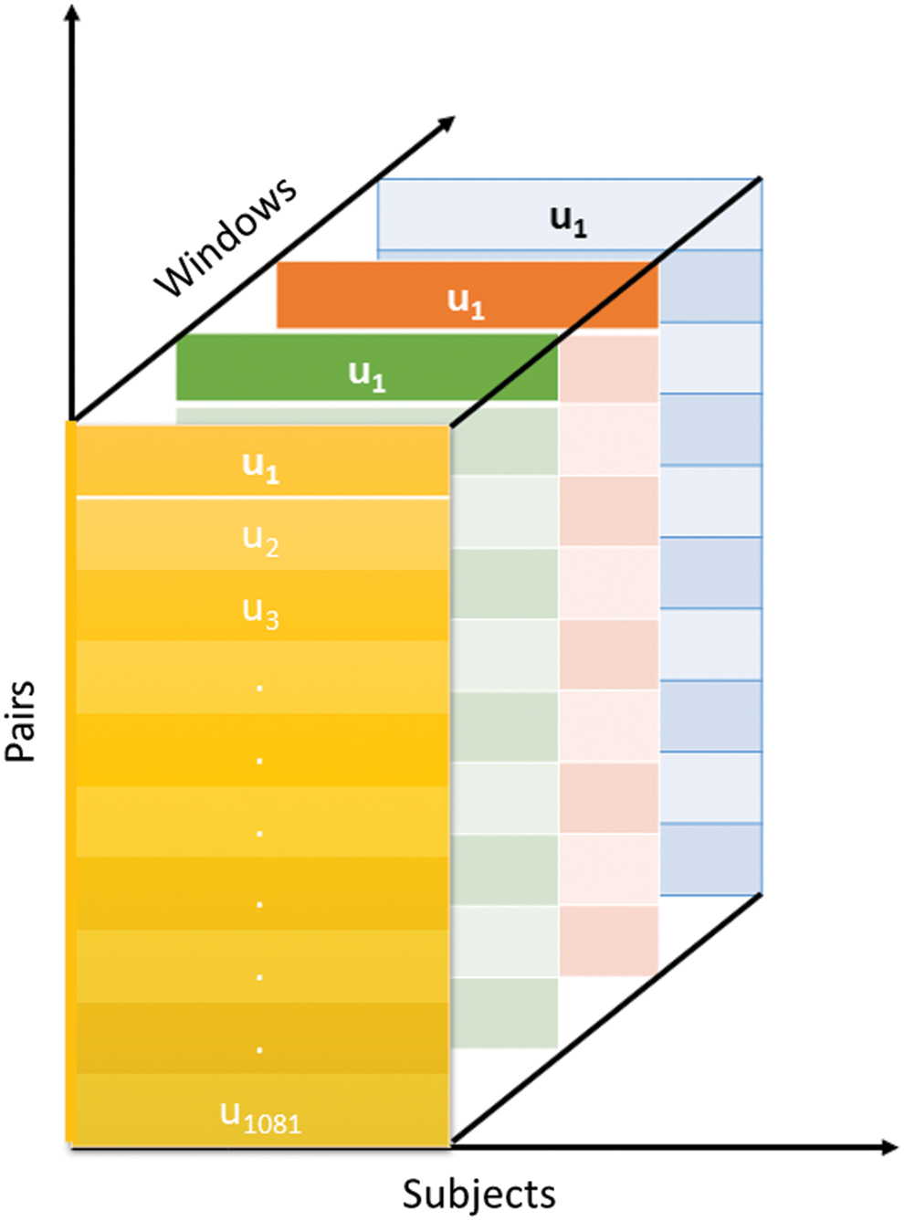
dFNC data set. Different color represents a distinct window, and each window has 1081 (u₁ to u₁₀₈₁) values, where the value represents the strength of connectivity between a pair of components. dFNC, dynamic functional network connectivity. Color images are available online.

Computing dFNC states

The subject-wise time course has a length of 136 windows, and a window consists of 1081 pairs where each pair represents a functional connection between two independent brain networks scaled from −1 to 1 (correlation). Of 100 ICA components, 47 are reported as relevant intrinsic brain networks in the earlier studies (Allen et al., 2014; Damaraju et al., 2014), generating a 47 × 47 symmetric matrix of connectivity. Thus, by taking either part of the diagonal, we obtain a vector of component pairs of size 1081 (⁴⁷C₂). To approximate the dFNC states, we collect windows from all subjects and run k-means clustering using Euclidean as a distance measure with an optimal k. We used the elbow criteria for selecting the model order (k), the within-cluster ratio between cluster distances, as suggested in previous studies (Abrol et al., 2017; Miller et al., 2016; Saha et al., 2019). We observe elbow for k = 5 (Fig. 3). We describe these window clusters as “k” different dFNC states. A state is consisting of a subset of subjects having at least one window included in that cluster. So, a subject can be included in the maximum k number of states and a minimum in one state.

FIG. 3.

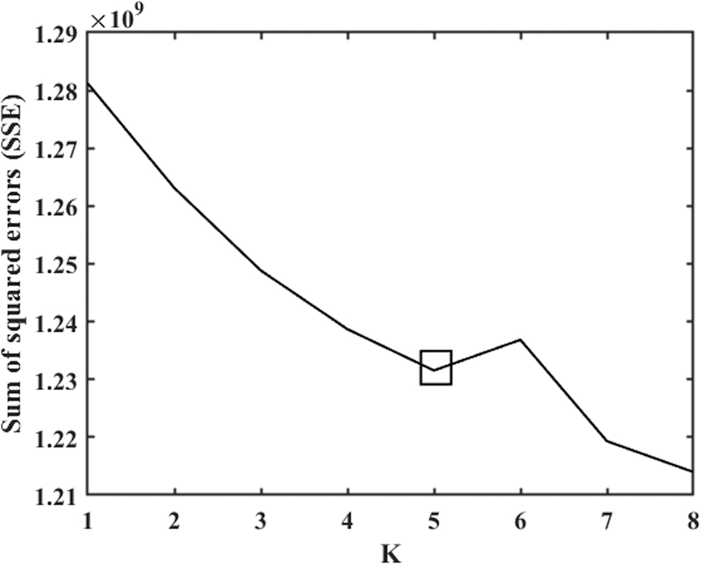
The elbow criteria for determining the model order (k) for k-means. We run k-means for k = 1 to 8. y-Axis represents the SSE for each k in the x-axis. The rectangular box indicates the elbow at k = 5. SSE, sum of squared errors.

Sorting the states

Given the k-means objective, windows within a state are expected to be analogous in connectivity patterns. However, k-means consider all the windows in a subject's time course, and each window potentially represents a connectivity signature span throughout the neural system. Thus, it is desirable to further summarize these states for a subset of windows highly correlated to the centroid of the corresponding state/cluster. The main objective is to maximize the homogeneity across the attributes of the states. In this study, we use the following heuristics to select closely associated widows and pairs that show low variance across the subjects within a window. We described both sorting techniques elaborately in the following paragraphs.

Sorting subjects within a state (maximizing the correlation)

For each subject s in a state k, the method computes a mean window across all the windows of type k in s that we describe as the mean window ( $μ W$ ). Next, it evaluates the Spearman correlation ( $α$ ) between $μ W$ and the centroid of the state, C_k . The heuristic computes this correlation $α$ for all the subjects in the state and takes an average of it, defined as a mean association score ( $μ α$ ) for that state. Finally, the process uses the following equations to retain a subgroup of subjects with a higher association. A subject is included in state S if, $c o r r (μ W, C) \geq μ α, w h e r e μ W = \frac{1}{| W |} \sum_{i = 1}^{| W |} W i,$

where $|W|$ is the number of windows of the subject included in state k, C is the centroid of a cluster, and “corr” is a MATLAB function for computing correlation between two vectors.

Sorting the pairs within a state (minimizing the variance)

In this study, the approach optimizes a subset of network pairs for the window that shows similar connectivity patterns beyond all state subjects. A window is a collection of pairs of networks (1081 in our case), and after sorting, the windows become a vector of size ≤1081. The algorithm evaluates variance ( $σ^{2}$ ) across all the subjects for each pair, which yields 1081 variances. Then, it calculates the mean of variances ( $μ σ^{2}$ ). Our heuristic keeps the pairs that are showing relatively lower variance across the sorted subjects. The following equation depicts the idea; a pair p is included in state S if, $σ^{2} < μ σ^{2}$

σ^{2} = v a r (\prod_{k = 1}^{n} W_{p, k}),

where $W_{p, k}$ represents $p t h$ value in $k t h$ window and n correspond to the number of windows in the state S.

Clustering the sorted states

The third step is exploring all possible subsets of sorted dFNC states. We propose a modified depth-first search (mDFS) (Even, 2011) for performing an exhaustive search toward generating all possible subsets of states.

mDFS core subroutine

The core part of the implementation is inspired by the popular depth-first-search algorithm (Kozen, 1992) for graph traversal. Typically, it discovers all possible connections among the nodes for a given set of nodes by traversing each node at least once. In our case, for a given set of states, we are interested in the relations (commonalities) between the subspaces. The relations might hold different sizes in terms of the number of states we are considering. So, the basic operation of our subroutine is an intersection among the features (subjects, windows, and pairs) of the states under consideration. Exploring the space by creating subsets is a straightforward solution to the problem; however, since we require to explore all possible subsets, it yields exponential growth in the time complexity. We propose a tweak in the DFS by considering the states as the nodes from an undirected graph and aim to establish edges (subset) based on satisfactory conditions on the input parameters. So, the major contribution is to add an early abandoning technique in DFS by restricting distinct parameters of the resulting subspace. Our proposed method (mDFS) requires a set of parameters given hereunder:

S: List of sorted states (ex: 1, 2, 3, 4, 5)

N: Minimum number of subjects in a tri-cluster

M: Minimum number of states/window cluster in a tri-cluster

P: Minimum number of pairs in a tri-cluster

O: Allowed percentage of overlap between two tri-clusters

It starts forming subsets of size 1 – n, where n is the number of states in the list. For a subset of states, first, it evaluates an intersection between their features to create a pseudo-cluster. Then, reporting that tri-cluster or extending it to more states depends on a validation step where the validator evaluates boundary conditions for N, M, and O. The DFS implementation uses backtracking for traversing the different branches of the search tree. The algorithm depends on the feedback from the validator to abandon a branch for exploration. The negative feedback leads the processing to an earlier branch of the search tree. Theoretically, the search complexity is of order O(2ⁿ). In practice, search space mostly becomes linear, an order of O(n). An example of an unsatisfied condition is that the number of subjects is less than N, or the overlap becomes greater than the threshold calculated based on O. Early abandoning a branch is feasible because the core operation in the searching process is an intersection. If the earlier iteration results in an inadequate tri-cluster (dynamic tri-cluster [dTiC]), there is no chance of obtaining a valid one in further steps. Therefore, the algorithm stops exploring the path and backtracks to an earlier point. For each eligible subset of states, we obtain an intersected 3D subspace consisting of a subset of states, subjects, and pairs. The validator computes the overlap ratio with the tri-clusters that have already been listed. In this study, we use the F ₁ similarity index to investigate the overlap between any earlier reported dTiCs (Hripcsak and Rothschild, 2005; Santamaria et al., 2007). The F ₁ similarity index is defined as follows for any two arbitrary tri-clusters A and B: $F 1 (A, B) = \frac{2 |A \cap B|}{|A| + |B|}$ $\begin{matrix} |A \cap B| & = I n t e r s e c t i o n b e t w e e n d T i C A a n d B; \\ S_{A \cap B} \times W_{A \cap B} \times P_{A \cap B} \end{matrix}$

\begin{matrix} |A| & = S i z e o f A; t h a t i s, t h e n u m b e r o f s u b j e c t s \\ \times w i n d o w s \times p a i r s \end{matrix}

\begin{matrix} |B| & = S i z e o f B; t h a t i s, t h e n u m b e r o f s u b j e c t s \\ \times w i n d o w s \times p a i r s . \end{matrix}

After traversing through the whole search space by mDFS, dNTiC returns a list of valid tri-clusters.

Parameter selection

k-Means yield five dFNC states; thus, the analysis assigns the minimum number of states parameter from 1 to 5. However, the dFNC state is a 3D substructure of subjects, pairs, and windows; thus, fusing more states leads to a shared subspace of neural features. Therefore, it is cardinal to set the appropriate input parameters for extracting meaningful subgroups. We first specify “O”—allowed percentage of overlap between the tri-clusters (dTiCs) to optimize the parameters. We explore a range of scalers for that parameter, which controls overlap among extracted dTiCs. Users can tweak this knob around to perturb the analysis; in our case, we tried a range from 5 to 35. The choice is vastly dependent on the data set, the number of subjects included in the sorted states, and the average overlap in subjects between the states (after k-means). However, these accessible selections are influenced by the remaining subjects, pairs, and windows in the sorted states. Table 1 shows the subgroups before and after sorting the states according to steps A and B. In our case, state 3 has the minimum number of subjects (S = 73), so intersection with this state can yield a maximum of 73 subjects in a dTiC if all the subjects match with other comparing states. However, for generalization, after multiple runs, we set them to moderate numbers, for example, N = 50, M ≤ 2, O ≤ 20%, and P = 500. In our case, we are clustering in three dimensions across the states. So, the tri-clusters quickly get narrowed down while we intersect the pairs of components and the subjects of multiple states. These parameters act as a subset of gears to explore the subspace for different objectives. For more than two states, the tri-clusters are reduced significantly in size. We tried setting the aforementioned parameters (N, M, P, and O) in many combinations by running the model for several repetitions and presented the results using the most stable setup. We present results on dTiCs that include a single state since the sorting steps already downsize the collection of features to a significant degree. So, these tri-clusters can provide imperative results on connectivity signatures and group differences. The parameters selection and use cases are partially explained in Rahaman and associates (2020).

Table 1.

Characteristics of the Sorted Dynamic Functional Network Connectivity States

States	Subjects		Pairs of components		Windows
States	Before sorting	After sorting	Before sorting	After sorting	Before sorting	After sorting
1	156	81	1081	619	4923	3582
2	251	159	1081	604	15,609	9156
3	146	73	1081	572	6071	3276
4	182	119	1081	576	8837	4907
5	163	97	1081	560	7264	3602

The table demonstrates the number of subjects, pairs of components, and windows included in the dynamic functional network connectivity states before and after running the sorting process (steps 1 and 2 of our methodology).

Results

We run the experiments using distinct combinations of input parameters for dNTiC approach. The significant results are presented in the following section and provide results from the extended investigation in our Supplementary Data. Our method extracts five tri-clusters (dTiC) for the input argument N = 50, M = 1 and P = 500. Figure 4 presents the group differences identified from these tri-clusters by running a two-sample t-test on each pair of components. In two upper rows, most of the dTiCs show higher connectivity in SC, VIS, SM, and default mode (DM) domains. The SC components show mild to moderate anticorrelation with AUD, VIS, and SM regions across the states and low negative to positive connectivity to all others.

FIG. 4.

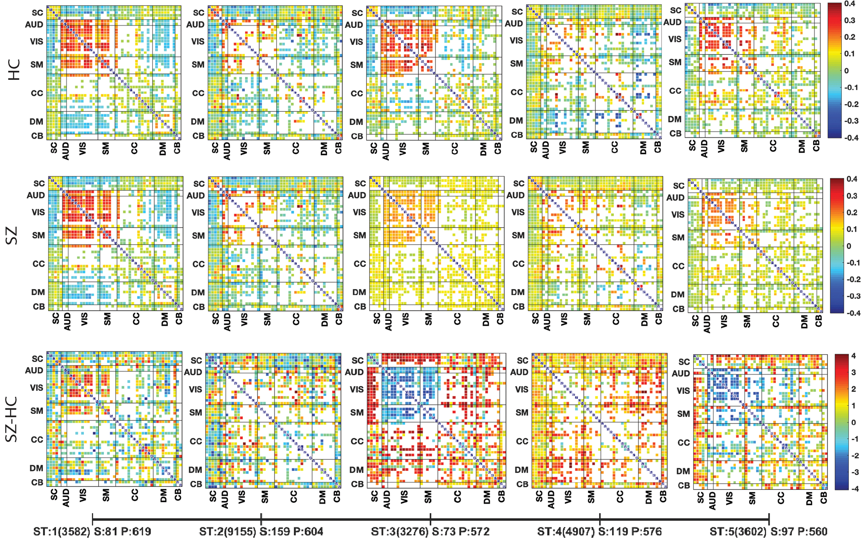
Group means (top two rows) and group differences (bottom row) of FC in distinct tri-clusters (dTiC). SZ and HC individuals are included in each dTiC. We evaluated the groupwise contribution on each pair of a dTiC by both groups. Two sample t-tests using a null hypothesis of “No group difference” we evaluate the statistical significance of the differences between patients versus the controls. A higher t-value indicates the rejection of the null hypothesis irrespective of their sign. However, the sign of t-values represents the directionality of the group difference. The pair matrix (47 × 47) is labeled into seven different brain domains subcortical, AUD, VIS, SM, CC, DM, and cerebellar, respectively. The white cells in the matrix indicate either the absence of that pair or nonsignificant group differences. The Xticklabel represents tri-cluster STs; the number of windows (of type ST) in that cluster from all the subjects included S: number of subjects in this dTiC; P: number of pairs included. These are the FDR corrected differences. AUD, auditory; CC, cognitive control; DM, default mode; dTiC, dynamic tri-cluster; FC, functional connectivity; FDR, false discovery rate; HC, healthy control; SM, sensorimotor; ST, state; SZ, schizophrenia; VIS, visual. Color images are available online.

dTiC 3 is the subgroup that shows substantial group differences among all the estimated dynamic tri-clusters. dTiC 1 and 3 distinguish each other in default mode network (DMN) connectivity (anticorrelated strongly to VIS and Motor in 1 vs. 3). dTiC 3 and 5 differ in SC connectivity to other domains, and dTiC 2 and 4 also distinguish each other in DMN connectivity. Apparently, dTiC 1, 3, and 5 have more active pairs in VIS and SM regions than dTiC 2 and 4. However, dTiC 2 and 4 have lightly more pairs in the cognitive control (CC) region. These are dTiC of subjects and pairs where one group of tri-clusters (dTiC 1, 3, and 5) is more active/dense across different regions. In contrast, another group (dTiC 2 and 4) is sparsely active, which means fewer pairs clustered together in those subjects.

The bottom row (of Fig. 4) demonstrates the group differences reported by the dTiCs. In dTiC 1, we can see pairs from SZ individuals showing higher connectivity strength than HC pairs in VIS and SM regions. dTiC 2 is sparse primarily in the different areas except for SZ-HC hyperconnectivity in DMN and CC. In contrast, dTiC 3 shows group differences across several regions of the brain. In this study, HC is showing a more substantial within domain connectivity in VIS, AUD, and SM regions, and greater anticorrelation to SC and CC nodes comparing with SZ. The directionality in the VIS-SM region is HC > SZ, and others are reverse. We find strong group differences in SC to AUD-VIS-SM domains, and it is higher correlations in the SZ group and lower in HC. Patients exhibit reduced connectivity (in this case, lack of anticorrelation) compared with HC. We also observe group differences in FC from DM to all other domains that evidently affect SZ in the subject's neural system. dTiC 4 shows significant differences in DM-VIS, CC, and dTiC 5 shows group differences in connectivity in SC to all other domains. The last dTiC is similar to dTiC 3 unless both distinguish each other in CC components. In essence, SC, sensory, DM, and CC regions revealed significant differences in average connectivity strength between patients and controls. In an analysis where we forced dNTiC to explore homogeneity across more than two states, we observed a large and significant tri-cluster (dTiC 4) where states 4 and 5 were clustered together and showed significant group differences in sensory and DM regions. We explain this scenario in the Supplementary Data.

Now, we evaluated the transition of each subject throughout these 3D homogenous dynamic patterns. We measure window frequency for each subject, representing how frequently a subject changes its pattern and how long it continues with the same pattern. In Figure 5, we computed each subject's window frequency within a tri-cluster, representing the percentage of windows type “i” for that subject. A subject can be a member of multiple tri-clusters. For a subject taken from dTiC “i”, we compute the percentage of the window of type “i”, which is also the amount of time in TR the subject spends in state “i”. These negative t-values are evident that window frequency in SZ subjects is smaller than in HC. Thus, HC subjects linger within uniform connectivity states, whereas SZ subjects move back and forth among relatively shorter states. However, of the dFNC time course, SZ subjects in dTiC 2 have more windows of type 2, which evidence these subjects' dynamics spent more time in state 2 than the HC subjects within. Overall, the results demonstrate that a quicker transition among different connectivity states better characterize SZ subjects.

FIG. 5.

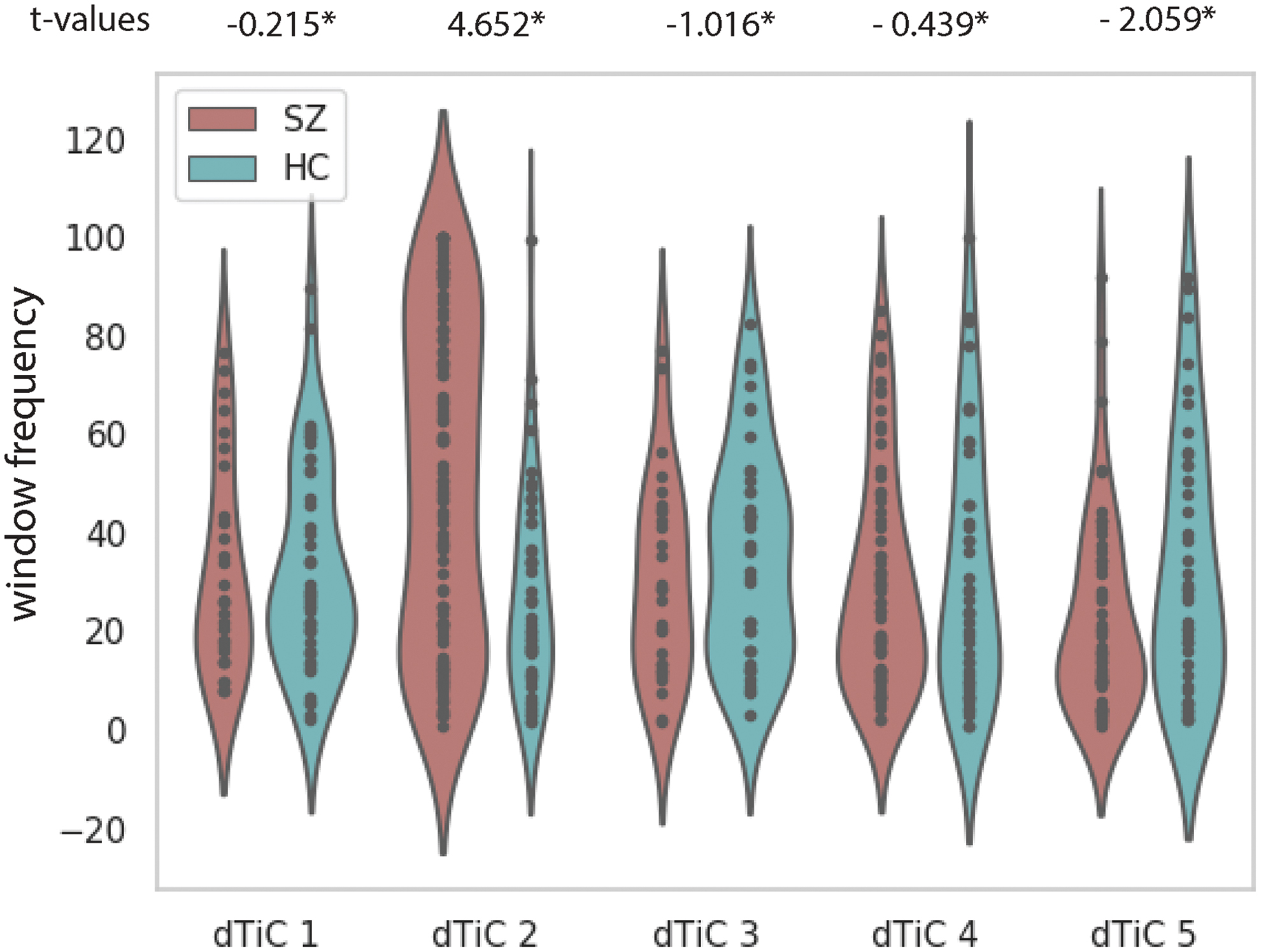
SZ–HC t-values from a two-sample t-test computed on window frequency in each subject within the tri-cluster. Window frequency is defined as the percentage of a specific type of window in a subject. The violins demonstrate the distributions of the data points. The asterisk sign on the t-value indicates the statistical significance at a level of p < 0.05. Color images are available online.

We check the correlation between mean FC and the positive and negative syndrome scale (PANSS) score from the SZ subjects to investigate if these patterns are related to the symptoms of the disorder (Kay et al., 1987). The regression line characterizes the pattern of symptom scores (positive, negative, and general) with the average connectivity strength of the patients included in a subgroup. We see from Figure 6, dTiC 1 anticorrelated with positive and associated with adverse symptoms; subjects in dTiC 2 express general symptoms, and the corresponding regression line demonstrates linear increment with the rise of connectivity. The general symptoms in dTiC 3 decreases with the increase of connectivity (the green line). We also observed weaker connectivity strength in the sensory, cerebellum, and motor region for the subjects included in that tri-cluster (Fig. 4). The loose connection of these regions is consistent with the general symptom measures in the PANSS scale, including tension, motor retardation, and anxiety. Moreover, the subgroup expresses more positive symptoms with higher connectivity, and for the negative symptoms, it follows the opposite. SZ subjects in dTiC 4 show a moderate correlation with negative PANSS scores. The symptoms are expressed more strongly with the increase of connectivity, a unique pattern within this subgroup. In general, for dTiC 4 and 5, the connectivity pattern in these subjects demonstrate the negative and positive symptoms, respectively. In dTiC 4, negative symptoms are raised with the increase of connectivity strength. So, the subset of pairs of components included in the tri-cluster map a few domains in the brain where the weaker connectivity might help control the negative symptoms in SZ. Finally, dTiC 5 also exhibits an association with positive symptoms, which manifest with higher connectivity. Although the associations are not very strong in terms of the correlation value, these indicate trends depicting interactions between the symptom scores and the connectivity strength within the subgroups. Thus, stronger connectivity in dTiC 5 may help protect against positive symptoms.

FIG. 6.

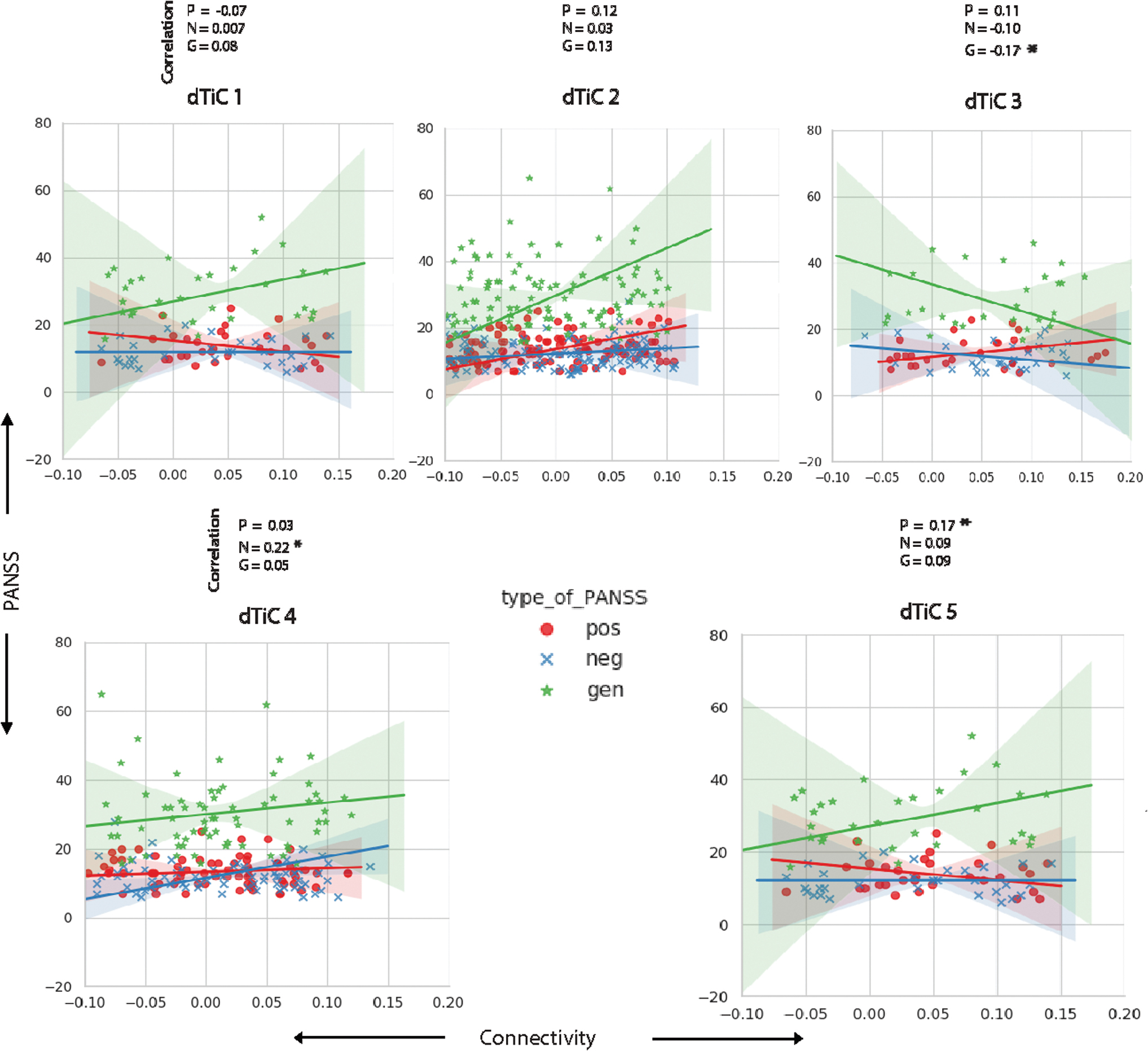
Correlation between PANSS score and mean connectivity strength for SZ subjects within each subgroup (dTiC). The subplots represent the data points and the regression lines between the variables. We plotted mean connectivity (x-axis) versus PANSS score (y-axis). In subgroup 1, the SZ subjects are anticorrelated with positive symptoms—the positive PANSS scores decrease with the rise of connectivity strength. Mentionable, these subjects show higher connectivity in VIS and SM regions (Fig. 5). Subjects in dTiC 3, 5 are highly correlated with positive symptoms and exhibit lower connectivity strength than controls within these subgroups. Patients in dTiC 3 show slightly diminishing trends in negative PANSS scores with the increase of their connectivity level. Anticorrelation with negative PANSS scores might indicate functional dysconnectivity in AUD, VIS, and SM regions (Fig. 5) effect negative symptoms in SZ. dTiC 4 has a strong association with negative symptom scores and show very sparse connectivity in VIS and SM regions (Fig. 5). The significant correlations are indicated using the asterisk sign. PANSS, positive and negative syndrome scale. Color images are available online.

Figure 7 presents the group differences in each state's reoccurrence time between patients and control. The reoccurrence time of a tri-cluster is given by the number of windows assigned to that dTiC. So, from a subject's windows, how many are assigned to a tri-cluster is the reoccurrence time. The definition is consistent with the earlier study (Li et al., 2017). Two-sample t-tests reveal dTiC 2 and 5, showing statistically significant (at a level p < 0.05) group differences in the reoccurrence time. We observe SZ subjects show a higher reoccurrence time for dTiC 3 but a lower reoccurrence time in dTiC 5. It indicates the connectivity pattern depicted by dTiC 2 is comparatively more recurring in SZ subjects than any other connectivity pattern.

FIG. 7.

Reoccurrence time of both SZ and HC subjects included in each dTiC. The green and red circles represent the reoccurrence time of HC and SZ subjects, respectively. The red line on the box shows the population mean—the asterisk sign indicates the dTiC with statistically significant differences between SZ and HC groups. We run a two-sample t-test on the reoccurrence time of SZ and HC subjects within a tri-cluster to evaluate the group differences. Subjects in dTiC 2 and 5 show statistical significance at a level of p < 0.05. Color images are available online.

Discussion

The study demonstrates a novel method of tri-clustering dFNC that sifts through all three dimensions of the data (network pairs, windows, and subjects) simultaneously. dNTiC provides a means of subgrouping the data more precisely, revealing significant complex relationships within the subgroups that do not exist across the dimensions. The study's outcomes are intriguing because, throughout the method, we maximized the homogeneity across the elements within a tri-cluster. Then we analyzed those highly homogenous subspaces for patient–control group differences, making the reported outcomes of the comparison more sensitive and meaningful. The results reveal significant differences in connectivity, coactivations, and antagonism across a set of distinct brain regions. We believe this illustrates a key strength of our approach; since relating PANSS symptoms to brain activity is challenging due to heterogeneity, the tri-clustering approach decomposes data instances into subgroups with more uniform subjects, connectivity values, and dynamic windows. Our initial thought was that this would enhance sensitivity to detect associations with subject variables such as symptom scores.

The observed group differences show how the connectivity strength differs in distinct regions of the brain of HC and SZ subjects. Subjects from tri-cluster 3 report distinguished group differences at distinct regions of the brain: a sharp antagonism in VIS and SM regions and less anticorrelation between SC and sensory networks. This subgroup also shows a higher correlation with positive symptom and anticorrelation with negative and general symptom scores, which indicates patient with hypoconnectivity in sensory (AUD, VIS, and SM) and hyperconnectivity between SC and sensory networks are more likely to express positive symptoms (i.e., hallucinations, delusions, and racing thoughts). These differences are prone to be related to sensory dysfunction in SZ, which has been linked to SZ symptoms such as AUD hallucinations and delusions (Javitt and Sweet, 2015; Rabinowicz et al., 2000; Zisook et al., 1999). The previous studies appear to reveal comparatively less FC differences within the brain regions (Allen et al., 2014; Barber et al., 2018; Du et al., 2017; Rashid et al., 2014). A potential reason for fewer differences could be the scattered focus throughout the brain. Our main contribution is building a more comparable subspace by reducing the heterogeneity across the characteristics of dFNC states. In addition to the group differences we presented, the subgroups of subjects are sorted across a third dimension: the number of pairs of components (connections). Instead of exploring the connectivity throughout the brain, different tri-cluster includes distinct subsets of connections. It assists in identifying subgroups of subjects (dTiC 2, 4) where a smaller number of pairs of components are present in (VIS, AUD, and SM) region than the tri-cluster dTiC 1, 3. The differences in the number of active connections in a region shed light upon the heterogeneity of connectivity structure and neural wiring in SZ.

That finer comparability helps to extract more group differences than earlier analysis. We can consider group differences in figure 3(B) (Allen et al., 2014), which used the same data set and followed the same preprocessing pipeline for a quantitative comparison. Apparently, our dTiCs provide more SZ–HC group differences in several domains. Their states report almost no differences except very sparse dots in AUD, VIS, and SM regions. For reference, we are providing figure 3(B) from that study in our Supplementary Data (Supplementary Fig. S3). In our research, the tri-clusters are more precisely sorted for a subset of subjects showing minimum heterogeneity in their connectivity pattern and show significant group differences across multiple brain regions. From Figure 4, we can see that all the dTiCs include a subset of subjects, which comprises one-third of the total number of subjects (N = 314) and half of the total number of pairs (N = 1081). This type of subgrouping of subjects and pairs can illuminate domain-wise connectivity differences within patients and control, which would be lost in a study using standard k-means or any other conventional clustering approaches (Allen et al., 2011, 2014; Miller et al., 2016; Rashid et al., 2014). The findings from the window frequency experiment characterize patients with a higher transition frequency across distinct connectivity states. This sporadic showcase of SZ dynamics also aligns with the previous investigation (Allen et al., 2011, 2014). Furthermore, when we ran the model using an increased number of states in a tri-cluster, which is at least two states (≥ 2) (Supplementary Data), which highlights the changes in connectivity strength for the extended subgroup that includes multiple states. The intuition behind mounting multiple states in each tri-cluster is to capture more extended connectivity patterns, which approximates the persistence of the states across the time course. However, the broader tri-clusters report less significant variations in the connectivity pattern than replicating the older templates among a smaller subset of connections/pairs of components. We also run the analysis for larger model order (k = 9) where we observe tri-clusters consistent with modeling order 5, indicating starting with more dFNC states eventually converges to the similar connectivity patterns we have already extracted using a smaller k.

Conclusion and Future Directions

Studies of FC data have primarily ignored individual variabilities and have not optimized across the multiple data dimensions. We are looking for clusters in the data set, showing a relation among the data variables while ensuring the subgroup's homogeneity. Moreover, it is useful to unveil biomarkers for mental disorders that are heterogeneous, such as SZ. The human brain is a complex dynamical system that experiences a vast array of events in a very short temporal modulation. Therefore, gazing at the dynamic entirely and searching for connectivity patterns throughout the entire system is a less intuitive way to explore. Our framework addresses issues in existing dFNC analysis methods; it searches for connectivity patterns that are more spatially constrained, often across a smaller subset of brain networks. By calibrating the size parameter of the algorithm, we can also analyze a feature's stability. For instance, if we identify a feature within a subgroup and gradually increase the number of states, we can test the longevity of this trend for a greater subset of states. Thus, dNTiC helps identify a connectivity signature and draw an approximate effect size for this. Our framework is dependent mainly on the selection of input parameters. We are developing a probabilistic framework to select these arguments for dNTiC algorithm based on the given information and other inferences as a future plan. We are also planning to extend the method for task-based fMRI data in which the windows would be synchronous across the subjects; thus, we can directly tri-cluster the data without applying k-means that will potentially increase the robustness of the algorithm. We are working on a Gaussian kernel-based exploration to identify the coactivation of connectivity patterns across the subjects over time for the sorting steps.

Footnotes

Authors' Contributions

V.D.C., M.A.R., and E.D. developed the idea. Data preprocessing was performed by E.D. The method was developed by V.D.C. and M.A.R. J.A.T., T.G.M.E., D.M., and J.V. helped to collect the data and to interpret the results. Authors B.M. and G.P. helped to interpret the results and writing the article. M.A.R., E.D., and V.D.C. designed the experiments and carried out the statistical analysis. All the authors edited the article substantially and contributed to different experimental phases; approved the final version of the submission.

Author Disclosure Statement

No competing financial interests exist.

Funding Information

This study was supported by the National Institutes of Health grants R01MH094524, R01MH118695, and R01EB020407.

Supplementary Material

Supplementary Data

Supplementary Figure S1

Supplementary Figure S2

Supplementary Figure S3

References

Abrol

, Damaraju

, Miller

, et al. 2017. Replicability of time-varying connectivity patterns in large resting state fMRI samples. NeuroImage, 163:160–176.

Allen

, Damaraju

, Plis

, et al. 2014. Tracking whole-brain connectivity dynamics in the resting state. Cereb Cortex, 24:663–676.

Allen

, Erhardt

, Damaraju

, et al. 2011. A baseline for the multivariate comparison of resting-state networks. Front Syst Neurosci, 5:2.

Alnæs

, Kaufmann

, van der Meer

, et al. 2019. Brain heterogeneity in schizophrenia and its association with polygenic risk. JAMA Psychiatry, 76:739–748.

Arieli

, Sterkin

, Grinvald

, et al. 1996. Dynamics of ongoing activity: explanation of the large variability in evoked cortical responses. Science, 273:1868–1871.

Barber

, Lindquist

, DeRosse

, et al. 2018. Dynamic functional connectivity states reflecting psychotic-like experiences. Biol Psychiatry Cogn Neurosci Neuroimaging, 3:443–453.

Beckmann

, DeLuca

, Devlin

, et al. 2005. Investigations into resting-state connectivity using independent component analysis. Philos Trans R Soc Lond B Biol Sci, 360:1001–1013.

Calhoun

, Adali

, Pearlson

, et al. 2001. A method for making group inferences from functional MRI data using independent component analysis. Hum Brain Mapp, 14:140–151.

Calhoun

, Kiehl

, Pearlson

. 2008. Modulation of temporally coherent brain networks estimated using ICA at rest and during cognitive tasks. Hum Brain Mapp, 29:828–838.

10.

Cetin

, Houck

, Rashid

, et al. 2016. Multimodal classification of schizophrenia patients with MEG and fMRI data using static and dynamic connectivity measures. Front Neurosci, 10:466.

11.

Damaraju

, Allen

, Belger

, et al. 2014. Dynamic functional connectivity analysis reveals transient states of dysconnectivity in schizophrenia. Neuroimage Clin, 5:298–308.

12.

Damoiseaux

, Rombouts

, Barkhof

, et al. 2006. Consistent resting-state networks across healthy subjects. Proc Natl Acad Sci U S A, 103:13848–13853.

13.

, Fu

, Sui

, et al. 2020. NeuroMark: an adaptive independent component analysis framework for estimating reproducible and comparable fMRI biomarkers among brain disorders. Neuroimage Clin, 28:102375.

14.

, Pearlson

, Lin

, et al. 2017. Identifying dynamic functional connectivity biomarkers using GIG-ICA: application to schizophrenia, schizoaffective disorder, and psychotic bipolar disorder. Hum Brain Mapp, 38:2683–2708.

15.

Erhardt

, Rachakonda

, Bedrick

, et al. 2011. Comparison of multi-subject ICA methods for analysis of fMRI data. Hum Brain Mapp, 32:2075–2095.

16.

Even

. 2011. Depth-first search. In: Even G (ed.) Graph Algorithms. Cambridge: Cambridge University Press; pp. 46–64.

17.

Ferri

, Ford

, Roach

, et al. 2018. Resting-state thalamic dysconnectivity in schizophrenia and relationships with symptoms. Psychol Med, 48:2492–2499.

18.

Franco

, Pritchard

, Calhoun

, et al. 2009. Interrater and intermethod reliability of default mode network selection. Hum Brain Mapp, 30:2293–2303.

19.

Friedman

, Hastie

, Tibshirani

. 2008. Sparse inverse covariance estimation with the graphical lasso. Biostatistics, 9:432–441.

20.

, Tu

, Di

, et al. 2018. Characterizing dynamic amplitude of low-frequency fluctuation and its relationship with dynamic functional connectivity: an application to schizophrenia. NeuroImage, 180:619–631.

21.

Hindriks

, Adhikari

, Murayama

, et al. 2016. Can sliding-window correlations reveal dynamic functional connectivity in resting-state fMRI?. NeuroImage, 127:242–256.

22.

Hripcsak

, Rothschild

. 2005. Agreement, the f-measure, and reliability in information retrieval. J Am Med Inform Assoc, 12:296–298.

23.

Ioannides

. 2007. Dynamic functional connectivity. Curr Opin Neurobiol, 17:161–170.

24.

Javitt

, Sweet

. 2015. Auditory dysfunction in schizophrenia: integrating clinical and basic features. Nat Rev Neurosci, 16:535–550.

25.

Kay

, Fiszbein

, Opler

. 1987. The positive and negative syndrome scale (PANSS) for schizophrenia. Schizophr Bull, 13:261–276.

26.

Keator

, van Erp

TGM

, Turner

, et al. 2016. The function biomedical informatics research network data repository. Neuroimage, 124(Pt B):1074–1079.

27.

Klugah-Brown

, Luo

, He

, et al. 2019. Altered dynamic functional network connectivity in frontal lobe epilepsy. Brain Topogr, 32:394–404.

28.

Kozen

. 1992. Depth-first and breadth-first search. In: Gries D (ed.) The Design and Analysis of Algorithms. New York, NY: Springer; pp. 19–24.

29.

Kucyi

, Davis

. 2014. Dynamic functional connectivity of the default mode network tracks daydreaming. NeuroImage, 100:471–480.

30.

Lawrie

, Abukmeil

. 1998. Brain abnormality in schizophrenia: a systematic and quantitative review of volumetric magnetic resonance imaging studies. Br J Psychiatry, 172:110–120.

31.

Leonardi

, Van De Ville

. 2015. On spurious and real fluctuations of dynamic functional connectivity during rest. NeuroImage, 104:430–436.

32.

, Zhang

, Liang

, et al. 2017. High transition frequencies of dynamic functional connectivity states in the creative brain. Sci Rep, 7:46072.

33.

, Calhoun

, Phlypo

, et al. 2014. Dynamic changes of spatial functional network connectivity in healthy individuals and schizophrenia patients using independent vector analysis. NeuroImage, 90:196–206.

34.

Makeig

, Debener

, Onton

, et al. 2004. Mining event-related brain dynamics. Trends Cogn Sci, 8:204–210.

35.

Miller

, Yaesoubi

, Turner

, et al. 2016. Higher dimensional meta-state analysis reveals reduced resting fMRI connectivity dynamism in schizophrenia patients. PLoS One, 11:e0149849.

36.

Onton

, Westerfield

, Townsend

, et al. 2006. Imaging human EEG dynamics using independent component analysis. Neurosci Biobehav Rev, 30:808–822.

37.

Rabinowicz

, Silipo

, Goldman

, et al. 2000. Auditory sensory dysfunction in schizophrenia: imprecision or distractibility?. Arch Gen Psychiatry, 57:1149–1155.

38.

Rahaman

, Turner

, Gupta

, et al. 2020. N-BiC: a method for multi-component and symptom biclustering of structural MRI data: application to schizophrenia. IEEE Trans Biomed Eng, 67:110–121.

39.

Rashid

, Arbabshirani

, Damaraju

, et al. 2016. Classification of schizophrenia and bipolar patients using static and dynamic resting-state fMRI brain connectivity. Neuroimage, 134:645–657.

40.

Rashid

, Chen

, Rashid

, et al. 2019. A framework for linking resting-state chronnectome/genome features in schizophrenia: a pilot study. Neuroimage, 184:843–854.

41.

Rashid

, Damaraju

, Pearlson

, et al. 2014. Dynamic connectivity states estimated from resting fMRI Identify differences among schizophrenia, bipolar disorder, and healthy control subjects. Front Hum Neurosci, 8:897.

42.

Saha

, Abrol

, Damaraju

, et al. 2019. Classification as a criterion to select model order for dynamic functional connectivity states in rest-fMRI data. In: 2019 IEEE 16th International Symposium on Biomedical Imaging (ISBI 2019). Venice, Italy: IEEE. DOI: 10.1109/ISBI.2019.8759146.

43.

Sakoglu

, Michael

, Calhoun

. 2009. Classification of schizophrenia patients vs healthy controls with dynamic functional network connectivity. Neuroimage, 47:S39–S41.

44.

Santamaría

, Quintales

, Therón

. 2007. Methods to bicluster validation and comparison in microarray data. In: Yin H, Tino P, Corchado E, Byrne W, Yao X (eds.) International Conference on Intelligent Data Engineering and Automated Learning. Heidelberg, Germany: Springer; pp. 780–789.

45.

Shakil

, Lee

C-H

, Keilholz

. 2016. Evaluation of sliding window correlation performance for characterizing dynamic functional connectivity and brain states. NeuroImage, 133:111–128.

46.

Shehzad

, Kelly

, Reiss

, et al. 2009. The resting brain: unconstrained yet reliable. Cereb Cortex, 19:2209–2229.

47.

Smith

, Miller

, Salimi-Khorshidi

, et al. 2011. Network modelling methods for FMRI. NeuroImage, 54:875–891.

48.

Tsuang

, Lyons

, Faraone

. 1990. Heterogeneity of schizophrenia: conceptual models and analytic strategies. Br J Psychiatry, 156:17–26.

49.

Turner

, Damaraju

, Van Erp

, et al. 2013. A multi-site resting state fMRI study on the amplitude of low frequency fluctuations in schizophrenia. Front Neurosci, 7:137.

50.

Varoquaux

, Gramfort

, Poline

J-B

, et al. 2010. Brain covariance selection: better individual functional connectivity models using population prior. Adv Neural Inf Process Syst, 23:2334–2342.

51.

Vergara

, Mayer

, Kiehl

, et al. 2018. Dynamic functional network connectivity discriminates mild traumatic brain injury through machine learning. NeuroImage Clin, 19:30–37.

52.

Wang

, Wang

, Huang

, et al. 2020. Abnormal dynamic functional network connectivity in unmedicated bipolar and major depressive disorders based on the triple-network model. Psychol Med, 50:465–474.

53.

Zisook

, McAdams

, Kuck

, et al. 1999. Depressive symptoms in schizophrenia. Am J Psychiatry, 156:1736–1743.

54.

Zuo

, Di Martino

, Kelly

, et al. 2010. The oscillating brain: complex and reliable. Neuroimage, 49:1432–1445.

Supplementary Material

Please find the following supplemental material available below.

For Open Access articles published under a Creative Commons License, all supplemental material carries the same license as the article it is associated with.

For non-Open Access articles published, all supplemental material carries a non-exclusive license, and permission requests for re-use of supplemental material or any part of supplemental material shall be sent directly to the copyright owner as specified in the copyright notice associated with the article.

0.00 MB

0.56 MB