Ensemble Learning for Multiple Sclerosis Disability Estimation Using Brain Structural Connectivity

Abstract

Background:

Multiple sclerosis (MS) is an autoimmune inflammatory disease of the central nervous system characterized by demyelination and neurodegeneration processes. It leads to different clinical courses and degrees of disability that need to be anticipated by the neurologist for personalized therapy. Recently, machine learning (ML) techniques have reached a high level of performance in brain disease diagnosis and/or prognosis, but the decision process of a trained ML system is typically nontransparent. Using brain structural connectivity data, a fully automatic ensemble learning model, augmented with an interpretable model, is proposed for the estimation of MS patients' disability, measured by the Expanded Disability Status Scale (EDSS).

Materials and Methods:

An ensemble of four boosting-based models (GBM, XGBoost, CatBoost, and LightBoost) organized following a stacking generalization scheme was developed using diffusion tensor imaging (DTI)-based structural connectivity data. In addition, an interpretable model based on conditional logistic regression was developed to explain the best performances in terms of white matter (WM) links for three classes of EDSS (low, medium, and high).

Results:

The ensemble model reached excellent level of performance (root mean squared error of 0.92 ± 0.28) compared with single-based models and provided a better EDSS estimation using DTI-based structural connectivity data compared with conventional magnetic resonance imaging measures associated with patient data (age, gender, and disease duration). Used for interpretation of the estimation process, the counterfactual method showed the importance of certain brain networks, corresponding mainly to left hemisphere WM links, connecting the left superior temporal with the left posterior cingulate and the right precuneus gray matter regions, and the interhemispheric WM links constituting the corpus callosum. Also, a better accuracy estimation was found for the high disability class.

Conclusion:

The combination of advanced ML models and sensitive techniques such as DTI-based structural connectivity demonstrated to be useful for the estimation of MS patients' disability and to point out the most important brain WM networks involved in disability.

Impact statement

An ensemble of “boosting” machine learning (ML) models was more performant than single models to estimate disability in multiple sclerosis.

Diffusion tensor imaging (DTI)-based structural connectivity led to better performance than conventional magnetic resonance imaging.

An interpretable model, based on counterfactual perturbation, highlighted the most relevant white matter fiber links for disability estimation.

These findings demonstrated the clinical interest of combining DTI, graph modeling, and ML techniques.

Introduction

Multiple Sclerosis (MS) is an immune-mediated inflammatory disease of the central nervous system, which causes demyelination and neurodegeneration with variable degrees of patients' disability (Ghasemi et al., 2016). While its etiology is still unknown (Polman et al., 2011), MS is the primary cause of nontraumatic neurological disability in young adults (Goodin, 2014). Its natural history includes a large heterogeneity of clinical symptoms and disease courses leading to cognitive deficits and irreversible disability (Lynch et al., 2005). In about 85% of cases, disease onset is characterized by a first acute episode called clinically isolated syndrome (CIS) and/or a relapsing-remitting course (RRMS), followed by a secondary-progressive course (SPMS), while the remaining 15% of patients starts directly from a primary-progressive course (PPMS) (Lublin et al., 2014). The clinical course of the disease and the risk to develop permanent disability are very different from one patient to another. Thus, to propose a personalized medical care and therapy, the neurologist's challenge is to predict the disease evolution based on early clinical, biological, and imaging markers available from disease onset.

The Expanded Disability Status Scale (EDSS) is the main test for quantifying disability and monitoring the disease progression over time (Kurtzke, 1983). Evaluated clinically by the neurologist, EDSS is an ordinal nonlinear rating scale that defines different levels of disability from 1 to 10, reflecting mostly walking and motor disability, and to a lesser extent cognitive impairment. In particular, eight functional systems are evaluated: pyramidal, cerebellar, brainstem, sensory, bowel and bladder, visual, cerebral, and other. These functional systems represent eight different areas of the central nervous system and each ranges from 0 (normal) to 5 or 6 (maximal impairment). These functional system grades, indications of mobility and restrictions in daily life, are used to define the EDSS as an ordinal measurement (Bushnik, 2011). For EDSS scores lower than 3, the disability remains moderate, while it becomes significant, affecting daily activities, for EDSS values of 3 to 4.5. With values over 5, the walking impairment becomes very severe and permanent (Van Munster and Uitdehaag, 2017). However, such neurological evaluation is limited by inter-rater reliability (Meyer-Moock et al., 2014).

MS disability prediction constitutes one of the most relevant aspects due to its impact on the decision therapy (Kuvalekar et al., 2015). Few machine learning (ML) methods have already shown their prognostic value based on conventional magnetic resonance imaging (MRI) (Kolcav et al., 2020, Law et al., 2019, Zhao et al., 2017), defined as measures for assessing inflammation (new and enlarging T2w lesions, gadolinium-enhanced T1w lesions), measures of acute and chronic disease (total T2 volume), and measures of degeneration (global brain and spinal cord atrophy, and chronic black holes on T1w images). Combined, they provide a unique insight into the dynamics of MS lesion development and the long-term pathological consequences on the central nervous system (Traboulsee et al., 2005). Tousignant et al. (2019) proposed an automatic end-to-end deep learning framework, based on parallel convolutional pathways, using multicenter MRI data images obtained in RRMS patients. Washimkar and Chede (2015) also used conventional MRI data images to identify lesions responsible for cognitive decline and physical disability. However, the poor correlation between inflammatory markers such as lesion load and patients' disability remains an issue (Declan and Trip, 2017).

More advanced MRI techniques, such as diffusion tensor imaging (DTI), was developed to provide a better characterization of the brain damages in MS, based on its great sensitivity to detect microarchitectural alterations in normal appearing white matter (WM) tissue (Jütten et al., 2019). Furthermore, new modeling approaches have been proposed to characterize the brain network organization by means of graph theory (Guo et al., 2017, Yong and Alan, 2010). These graph models consist of nodes, based on the parcellation of brain gray matter (GM) regions, and edges, determined by the underlying links between the network nodes. In brain structural connectivity, these links are defined by the extraction of WM fibers using DTI tractography (Basser et al., 2000). These new approaches laid the foundation for a better characterization of microarchitectural damages in MS (Bakshi et al., 2008). Such brain structural connectivity data were also used for ML techniques and provided excellent performances for the classification of MS clinical courses (Kocevar et al., 2016; Marzullo et al., 2019a) and the estimation of EDSS (Marzullo et al., 2019b). Nevertheless, the ensemble-based approach, where several models are combined together, demonstrated to be even more efficient compared with single-based models (Liu et al., 2004; Tsoumakas and Vlahavas, 2007). However, one of the drawbacks of ML models is their lack of transparency. Thus, several approaches were recently proposed (Gilpin et al., 2018) for model interpretability, first, to evaluate the accuracy of the decision strategy, and second, to understand the biological basis of the best results. This information is crucial for a better understanding of the pathological processes, their potential therapy, and to convey more trust in the results (Witten and Eibe, 2020).

In this work, we propose first a meta-learning approach, composed of four boosting base models organized in a stacking generalization scheme, to perform a cross-sectional estimation of disability (EDSS) in MS patients of different clinical courses. Second, a global and local interpretability model is developed to pin-down the brain connections that are most likely responsible for explaining different degrees of disability. The proposed approach benefits from both the sensitivity of DTI to detect microscopic WM alterations and the brain network connectivity model to point out disruptions of fiber links related to disability. In our knowledge, this is the first attempt to apply interpretable ML techniques to correlate brain structural connectivity with MS disability.

Materials and Methods

MRI acquisition

MRI examination was performed on a 1.5T Siemens Sonata system (Siemens Medical Solution, Erlangen, Germany) using an 8-channel head-coil. The conventional MRI protocol consisted of 3D T1-weighted MPRAGE (magnetization prepared rapid gradient echo) sequence (repetition time/echo time/time for inversion (TR/TE/TI) = 1970/3.93/1100 ms, flip angle = 15°, field of view (FOV) = 256 × 256 mm, voxel size = 1 × 1 × 1 mm³, acquisition time = 4.62 min) and a FLAIR (fluid attenuated inversion recovery) sequence (TR/TE/TI = 8000/105/2200 ms, flip angle = 150°, matrix size = 192 × 256, FOV = 240 × 240 mm, slice thickness = 3 mm, voxel size = 0.9 × 0.9 × 3 mm, acquisition time = 4.57 min). For DTI, an axial 2D spin-echo echo planar sequence was used (TE/TR = 86/6900 ms; 2 × 24 directions of diffusion gradient; b = 1000 s·mm⁻²; spatial resolution of 2.5 × 2.5 × 2.5 mm³).

Ninety MS patients distributed in four clinical courses (12 CIS, 30 RRMS, 20 PPMS, 28 SPMS) were recruited, following the (McDonald et al., 2001) diagnosis criteria, in the MS clinic of Lyon Neurological Hospital. Also, 15 healthy controls (HC) subjects, age- and gender-matched with MS patients, were included. Each patient received a clinical visit and an MRI examination, longitudinally, every 6 months during the first 3 years and then every year for the following 4 years. Patient information is provided in Table 1. A total of 528 scans were used in this study.

Table 1.

Data Set Information by Multiple Sclerosis Clinical Profiles (HC, CIS, RR, SP, PP)

	No. of subjects	No. of scans	Age	DD	EDSS (range)	Sex (% female)	Time scans
HC	15	15	35.7 (10.1)	—	—	57	—
CIS	12	56	29.9 (6.4)	3.1 (1.6)	1 (0–3)	52	248.5 (111.0)
RR	30	187	27.7 (7.8)	8.6 (4.1)	2.5 (0–4.5)	80	271.8 (101.6)
SP	28	160	29.1 (7.1)	14.7 (5.2)	5 (3–7)	39	266.0 (97.3)
PP	20	110	35.9 (5.1)	7.7 (3.2)	4 (2.5–6.5)	63	254.7 (96.2)

Data set information partition by MS clinical profiles. Age and DD are reported as average of years (standard deviation in parenthesis). The median was considered for the EDSS score (range in parenthesis). Time between scans was reported in days and the average was considered (standard deviation in parenthesis).

CIS, clinically isolated syndrome; DD, disease duration; EDSS, Expanded Disability Status Scale; HC, healthy controls; MS, multiple sclerosis; PP primary progressive; RR, relapsing remitting; SP, secondary progressive.

To offer a feasible interpretation of the model behavior, the output space (EDSS score) was partitioned into three levels of disability (low [1–3], medium (3–4.5], and high (4.5–7]) defined by our neurologist (F.D.D.) in agreement with the literature (Kurtzke, 1983). In Table 2, the information of the data set partitioned by EDSS classes is also provided.

Table 2.

Information on the Data Set by EDSS Groups (Low—Medium—High)

	No. of scans	No. of scans per patient	Age	DD	Sex (% female)	Time between scans
Low	169	4.1	27.5 (7.3)	6.00 (1.9)	75	264 (139–804)
Medium	201	4.5	31.9 (6.9)	10.67 (4.2)	62	250 (148–689)
High	143	4	30.4 (8.2)	13.04 (4.8)	48	279 (141–437)

Data set information partition by disability classes (low, medium, high). Age and DD are reported as average of years (standard deviation in parenthesis). Time between scans was reported in days and the average was considered (range in parenthesis).

EDSS, Expanded Disability status scale.

The proportion (%) of MS phenotypes in the three disability groups was distributed as follows: low: 100 HC and CIS, 58 RR; medium: 39 RR, 60 SP, and 58 PP; high: 40 SP and 36 PP. Inclusion criteria specified that excluded from this study are patients with contraindications to MRI (cardiac valve not compatible with MRI, claustrophobia, etc.), pregnant patients, patients requiring premedication for the examination, and patients with severe associated pathology or neurological disease other than MS, or any disabling condition that may interfere with the measurement of clinical disability and brain atrophy. Highly disabled patients with EDSS over 7 were also excluded from the study to select patients with less brain damages. This study was approved by the local ethics committee (CPP Sud-Est IV n° 2004-085) and the French national agency for medicine and health products safety (ANSM). Written informed consents were obtained from all patients before study initiation.

Image and graph processing

First, brain segmentation was performed on 3D T1-weighted images. Each voxel was classified into four classes: WM, cortical GM, subcortical GM, and cerebrospinal fluid using the FreeSurfer image analysis suite (Reuter et al., 2012). From GM maps, 84 regions (nodes) were identified based on the atlas Desikan for parcellation (Desikan et al., 2006) applied in common space. Second, DTI images were processed using the FMRIB Software Library (FSL; Jenkinson et al., 2012). Eddy current correction and nonbrain voxel stripping were performed as preprocessing steps. In each voxel of WM maps, the diffusion orientation distribution function (dODF) was computed using MRtrix software (Tournier et al., 2012). The maximum spherical harmonics of order-k was calculated by $(k + 1) (k + 2) ∕ 2 < d$ where d represents the number of acquisition diffusion directions (24) while k was set to 4. Constrained probabilistic streamline tractography was performed from dODF using the ACT package from MRtrix (Smith et al., 2012; Tournier et al., 2012). Third, an undirected weighted graph G = (V, E, ω) was defined, where |V| = q represents the set of nodes, |E| = m represents the set of connections between these nodes and ω defines the number of fibers connecting two nodes. By combining GM parcellation, with the ACT fiber-tracking of WM, the general connectivity matrix $A ε ℵ^{q x q}$ was obtained by summing the number of streamlines connecting each pair of nodes for a specific subject. More formally, let $a_{i j}$ be a general element of the matrix A where $1 < i, j < q$ , and q = 84, then the element $a_{i j}$ of A is defined by $\sum^{} : ℵ^{2} \to ℵ$ and represents the number of fibers connecting the node i with the node j.

Model conception

A stacked ensemble model, composed of multiple gradient boosting algorithms, was developed to estimate the disability status of MS patients, using their structural connectome. A thorough explanation of each phase of the workflow is given in the following section. The ANOVA statistical test of hypothesis was used to evaluate statistical differences (α < 0.05) in the estimation error between MS disability classes (low, medium, and high). In addition, to demonstrate the superiority of our approach, a comparison between the connectome data and conventional MRI measures was performed using three additional controlling factors (age, gender, and disease duration). Conventional MRI measures included WM T2w-lesion volume, lateral ventricle volume, cortical and subcortical GM volume, black hole T1w-lesion volume, obtained from T1w and FLAIR images using the MSmetrix software (Jain et al., 2015) developed by icometrix (Leuven, Belgium). Besides, our model included the development of an interpretability model based on the counterfactual concept and a conditional logistic regression. Figure 1 depicts the complete workflow of our model.

FIG. 1.

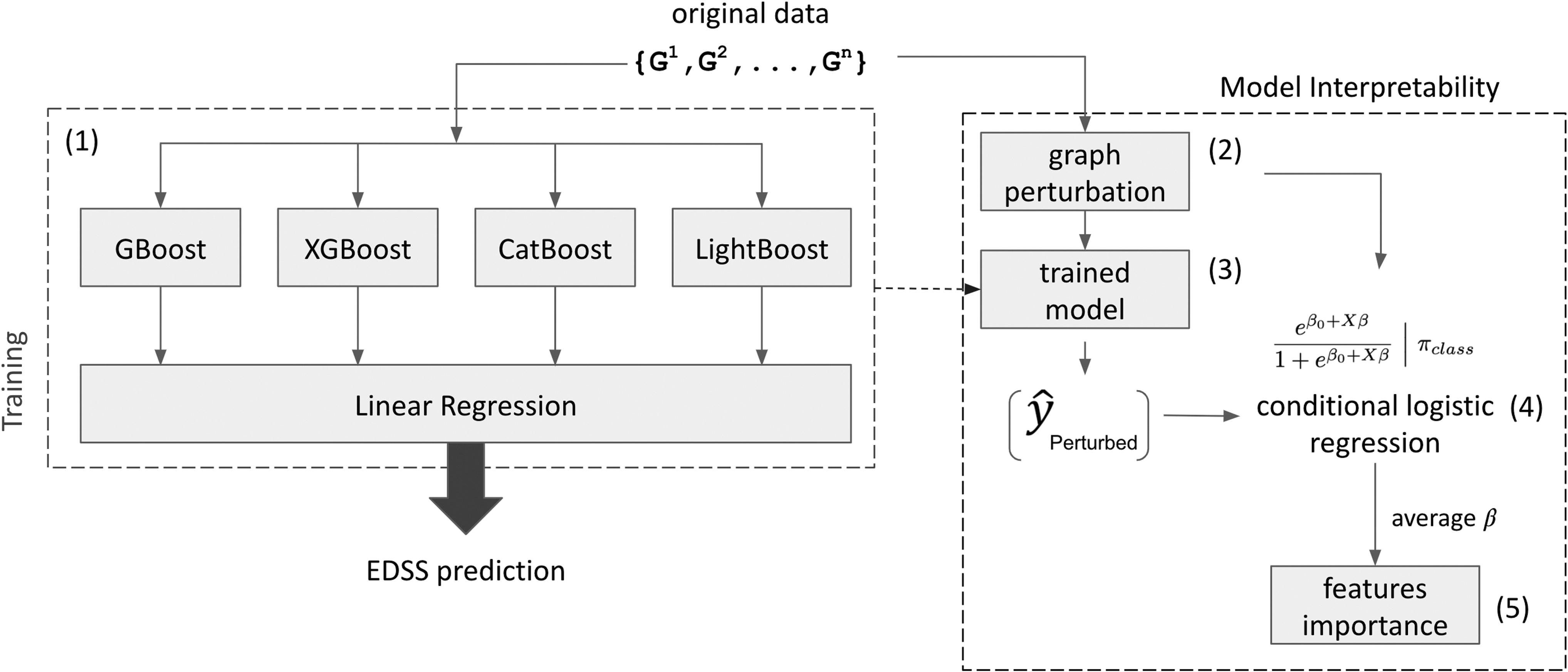
Complete model pipeline. The left box represents the training process of the stacked ensemble model, while the right box represents the interpretability model. (1) Starting from original data (WM connectivity matrix), the stacked ensemble model is trained to estimate the EDSS score. Notice that the original data set is only used for training and validating the model. (2) For each holdout set during the cross-validation, the original data set is perturbed to generate valid counterfactual WM connectivity matrix samples. (3) The perturbed (counterfactual) sample is used to probe the trained ensemble model and a corresponding counterfactual EDSS score is obtained (y_perturbed). (4) A statistical analysis based on the conditional logistic regression model is performed to estimate the β coefficients describing the importance of each link in the WM connectivity matrix of the generated counterfactual sample. (5) Conditioning on the disability class (low—medium—high), the β coefficients are averaged to obtain the final score of importance. EDSS, Expanded Disability Status Scale. WM, white matter.

The ensemble model is trained using the brain structural connectome data set in its adjacency matrix form (referred to as “original data” in Fig. 1). As shown in Figure 1, the green box encloses the training process for which an estimation of the EDSS score is obtained. Once the training process is completed, the final ensemble model is ready to be interpreted by the statistical model. The red box encloses the interpretability model. For each holdout sample, a graph perturbation, based on conditional probability distribution, is performed to obtain valid counterfactual samples. The perturbed (counterfactual) data set is used as input for the trained ensemble model to estimate the counterfactual EDSS score ( $ŷ_{p e r t u r b e d}$ ). The obtained counterfactual data set, combined with the EDSS estimation, is used by the statistical model to retrieve the causal effect of the WM fiber connections on the EDSS disability score. Finally, the average of the β coefficients, conditioned by disability classes, is considered to obtain the final score of importance.

Stacking generalization model for EDSS estimation

An ensemble model is an advanced ML approach where multiple single-base models are assembled to better predict an outcome. As long as the base models are diverse and independent, the variance of the prediction error decreases when the ensemble approach is used (Kotu, 2015). To combine the base models together, a stacked generalization scheme was applied. Basically, a meta-learning algorithm is built to learn how best to combine the predictions from multiple single-base ML algorithms. In our implementation, linear regression was used as the higher level model (Wolpert, 1992). The ensemble model is composed of four different gradient boosting algorithms. ML boosting techniques use subsequent sets of weak learners added together such that the residual error obtained from the previous learner is reduced. It relies on the intuition that the best possible next model, when combined with previous models, minimizes the overall prediction error. Gradient boosting exploits differentiable loss functions by using gradient descent approximation to minimize the objective function when adding subsequent learners. Moreover, the function that estimates $\hat{f}$ is parameterized in an additive functional form as follows:

where K represents the number of iterations, ${\hat{f}}_{0} (x)$ represents the starting model, and ${\{{\hat{f}}_{k} (x)\}}_{k = 1}^{K}$ defines the set of subsequent learners. The final model $\hat{f} (x)$ , obtained by sequentially training multiple learners on the residuals of the previous one, is the overall ensemble function. The optimization function is thus defined as follows:

where $h (x, θ)$ represents the subsequent base learner, $ρ$ defines the learning rate, and $g_{t} (x) = E_{y} = {[\frac{\partial Ψ (y, f (x))}{\partial f (x)}| x]}_{f (x) = {\hat{f}}^{t - 1}}$ (3)

while the loss function is defined as the squared-error L₂ loss: $Ψ {(y, f (x))}_{L_{2}} = \frac{1}{2} {(y - f (x))}^{2}$ (4)

Most often, a regularization term is added to the final loss function to avoid overfitting. In this context, the minimization objective becomes:

where $Ω (f)$ represents the regularization term, used for penalizing the complexity of the model, and defined as follows: $Ω (f) = ψ T + \frac{1}{2} λ ω$ (6)

where T defines the number of leaves in the tree and $ψ$ represents the corresponding weights, while the second term in the summation represents the L1 regularization. The additional term added to the final loss helps in smoothing the final learned weights to select a model, which is the simplest between those that perform the best on the test data. The four models considered in this study are as follows: gradient boosting machine (GBM) (Friedman, 2001), Extreme Gradient Boosting (XGBoost) (Chen and Guestrin, 2016), Categorical Gradient Boosting (CatBoost) (Veronika et al., 2018), Light Gradient Boosting (LightBoost) (Ke et al., 2017). Each of them exhibits a specific behavior for building trees and dealing with overfitting. In particular, while GBM subsamples rows before creating each tree, XGBoost subsamples both rows and columns for training each individual base learner and for the splitting strategy. LightBoost uses a novel technique of gradient-based one-side sampling to filter out the data instances for finding the optimal split value for building week-learner-trees, while XGBoost implements presorted histogram-based algorithms as a splitting strategy. Finally, CatBoost deals with the problem of prediction shift for which given a prediction model F the distribution of $F (x, k) | x_{k}$ leads to a shift from the distribution of $F (x) | x$ (Veronika et al., 2018). In this case, ordered boosting implementation, a modification of standard gradient boosting algorithm which avoids target leakage, is used.

Model interpretability

Following the first process of disability estimation, a counterfactual model was implemented to uncover the causal link between brain connections and disability. A counterfactual explanation describes a causal situation in which, if a specific event X had not occurred, a consequent event Y would not occur. In practice, counterfactual thinking requires a hypothetical situation that has in fact never happened. In other words, it provides a what-if explanation for model output. In this work, a counterfactual-based model is proposed with the aim of explaining the global and local behaviors of a general trained black-box model. This approach aims at investigating first, which features (graph connections) are more relevant for disability estimation (global), and second, how this role is varying with the level of disability (local). In other words, a local explanation is obtained by looking for features that explain a confined part of the output space. Similar to the global analysis, a local counterfactual explanation of a prediction can be interpreted as the smallest change to the feature values (hereafter feature perturbation) needed to obtain the output of interest.

Global interpretability

Global interpretability is first obtained by identifying the smallest number of important features that best explain the output prediction. For this purpose, we exploited the characteristics of the tree-based boosting methods, where the importance was calculated for each feature, at a single-tree level and averaged across all the trees of the ensemble (Hastie et al., 2009) as specified in the following equation:

where

In this formulation, $J - 1$ represents the number of internal nodes of the k-th tree, while $v (j)$ defines the l-th input feature and I represents the corresponding identity function. In other words, the importance of each feature was calculated averaging over all the maximal estimated improvements $î_{j}^{2}$ , defined in terms of reduction in entropy, for the l-th selected feature. In Layman's terms, a weighted frequency is calculated for a specific feature of each base model. The higher the number of times a specific feature is used, on average, by all the trees of the ensemble to make a splitting decision, the higher its importance is. To obtain a final common score, a normalization process is applied.

This approach is repeated for each boosting-based learner in the meta-model. For each base learner, only the features with a score of importance greater than the fifth percentile of not-null feature values are selected. Finally, to define a unique set of features, the union of all base-learner sets is considered. A threshold of importance, obtained through Equation (7), was set up to a value of 10%, corresponding to the exponential increase of the cumulative relative importance.

Local interpretability

A local counterfactual method refers to the technique that can explain the prediction results of the ML model depending on certain conditions. Three requirements need to be met:

1. prediction obtained from counterfactual should be as close as possible to the objective output;

2. counterfactual should be as similar as possible to the original instance, which translates in changing as few features as possible; and

3. counterfactual instance should have feature values that are likely.

For each disability level, a truncated normal distribution is assumed as described in Equation (8) $f (x; μ, σ, x_{1}, x_{2}) = \frac{1}{σ} \frac{ϕ (\frac{x - μ}{σ})}{ϕ (\frac{x_{2} - μ}{σ}) - ϕ (\frac{x_{1} - μ}{σ})}$ (8)

if $x_{1} < x < x_{2}$ and 0, otherwise where x ₁ and x ₂ define the upper and lower bounds of each distribution, respectively. The parameter $μ$ defines the center of the class, while $σ$ defines its dispersion. The applied strategy for constructing counterfactuals was based on input perturbations of patients' data (feature perturbation). It is important to notice that the conditional distribution in Equation (8) is only used to retrieve the final score to be optimized, expressed in terms of probability. In other words, given a patient in the center mass of the distribution of a specific disability class (low, medium, or high), the algorithm aims at “moving” the subject to the tail of the distribution without switching to a new class. Coherently, if the patient starts from the tail of the distribution, the perturbation moves him/her toward the center mass. This is equivalent to say that the probability of a patient to pertain to a specific class should decrease (or increase) in absolute value, under (or over) the threshold obtained by substituting the corresponding $μ \pm σ$ into Equation (8).

To satisfy the requirements for good counterfactuals, a conditional probability distribution was considered for applying perturbations. The mathematical formulation is given in Equation (9). $S_{x_{i, j, z}} = \{U_{d_{x_{1}}, d_{x_{2}}} |d_{x_{i, j, z}} \forall i ε 1, \dots,| d_{d_{x_{j, z}}}\}$ (9)

where $d_{d_{x_{j, z}}}$ defines the percentile distribution over the j-th edge and the z-th EDSS disability class, while $U_{d_{x_{1}}, d_{x_{2}}}$ represents the uniform distribution between the percentiles x ₁ and x ₂: $U_{d_{x_{1}}, d_{x_{2}}} = \{\begin{matrix} \frac{1}{x_{2} - x_{1}} \forall x_{i} ε [x_{1}, x_{2}] \\ 0, \forall x_{i} \underset{̲}{<} x_{i} | x_{i} \underset{̲}{>} x_{2} \end{matrix}$

which implies that the number of connections between x ₁-th and the x ₂-th percentiles is equally likely.

The goal is to perturb the lowest number of edges to increase (or decrease) the likelihood of a subject to make him/her more (or less) likely to pertain to a certain disability class of interest. This process ensures the first two requirements for a good counterfactual. To satisfy the third requirement, the conditional probability distribution was used to perturb the original input. This corroborates the idea of a highly likely counterfactual since it lies inside the manifold of the true data. An iterative process was then applied where, for each subject, one thousand counterfactuals were generated conditioning on the disability class. The causal effect of each edge onto the probability of pertaining to a predefined class of disability was obtained by conditional logistic regression [Eq. (10)]. $P (Y | X, β, π) = \frac{e^{β_{0} + X β}}{1 + e^{β_{0} + X β}}| π_{c l a s s}$ (10)

where $π$ defines the disability class of interest. The process was repeated for each patient, and the average of the $β$ parameters was considered.

Parameter setting and model evaluation

The model performance was evaluated using a 10-fold cross-validation strategy. At each cycle, nine folds were used for training and validation, using an 80–20% split strategy (nested cross-validation), determining the best hyperparameters for each base model by using a grid-search method, and the last fold was holdout for testing the performance of the final model. For each base model, only a limited number of parameters have been tuned. For all the boosting models, 300 trees were used except for the XGBoost model for which 500 trees were used. The learning rate was imposed to 0.2, while the maximum depth parameter was imposed to 3 for all the models, but for XGBoost 5 was used. All other parameters were left unchanged at their default values. Concerning the counterfactual model, the parameter $μ$ is imposed to be the center disability class value (low: 2, medium: 3.75, and high: 5.5), except for the high disability class for which a lower value was considered to compensate for its skewness. The $σ$ parameter was imposed to 0.5 for all the classes, except for the middle disability class for which 0.25 was used to keep the proportion unaltered.

Results were evaluated by calculating the root mean squared error (RMSE) [Eq. (11)]:

which measures the weighted average root squared difference between the estimated values and the measured value. Moreover, to avoid possible misinterpretations of the true predicting power due to outliers' errors, the mean absolute deviation error (MADE) was also considered [Eq. (12)]:

In both cases, the parameter $σ$ is imposed to be a unitary vector, while $\hat{f}$ defines the predicted value from the model and $μ$ the expected value.

Results

Stacking generalization model performance

The evaluation of the models' performances was assessed on both single and ensemble models using two types of data: the connectome-based data on one hand and on the other hand, conventional data including conventional MRI measures and patients' information (age, gender, and disease duration) (Table 3).

Table 3.

Ablation Study: Performance Comparison Between Single-Base Models and Stacking Ensemble

	CatBoost	GBM	XGBoost	LightBoost	LR	Stack
Graph	1.065 (0.264)	0.998 (0.269)	1.026 (0.312)	1.026 (0.287)	1.301 (0.185)	0.92 (0.278)
MRI+demographics	1.575 (0.456)	1.606 (0.437)	1.608 (0.422)	1.575 (0.384)	1.41 (0.376)	1.562 (0.405)
p	0.0013	0.0005	0.0008	0.0008	0.1967	0.0003

Performance comparison between single-base models and the stacked ensemble model. The values in the table report the average RMSE score (standard deviation in parenthesis) calculated over the same 10 folds of the cross-validation. LR was also considered for comparison. The first line of the table (Graphs) reports the performance comparison based on the connectome data. In the second line of the table (MRI+demographics), eight clinical measures were used for estimating EDSS (T2w lesion volume, T1w black hole volume, cortical GM volume, deep GM volume, lateral ventricles, age, sex, and disease duration). Last line reports the p-value comparison using the nonparametric Wilcoxon Mann–Whitney test.

GBM, gradient boosting machine; GM, gray matter; LR, linear regression; MRI, magnetic resonance imaging; RMSE, root mean squared error.

When comparing the two types of data, the performances were significantly different for all models with the exception of linear regression (p > 0.05), demonstrating the superiority of the DTI connectome data compared with the conventional data. Second, the stacking generalization model showed its superiority with respect to all single-base models by an overall RMSE of 0.92 (±0.28) and a MADE score equal to 0.8 (±0.7). This later suggested that a longer tail on the right-hand side of the error distribution was present. A more detailed performance analysis of the ensemble model with graph data was conducted along with the disability levels. As shown in Figure 2, the error distribution was reported for low, medium, and high disability classes.

FIG. 2.

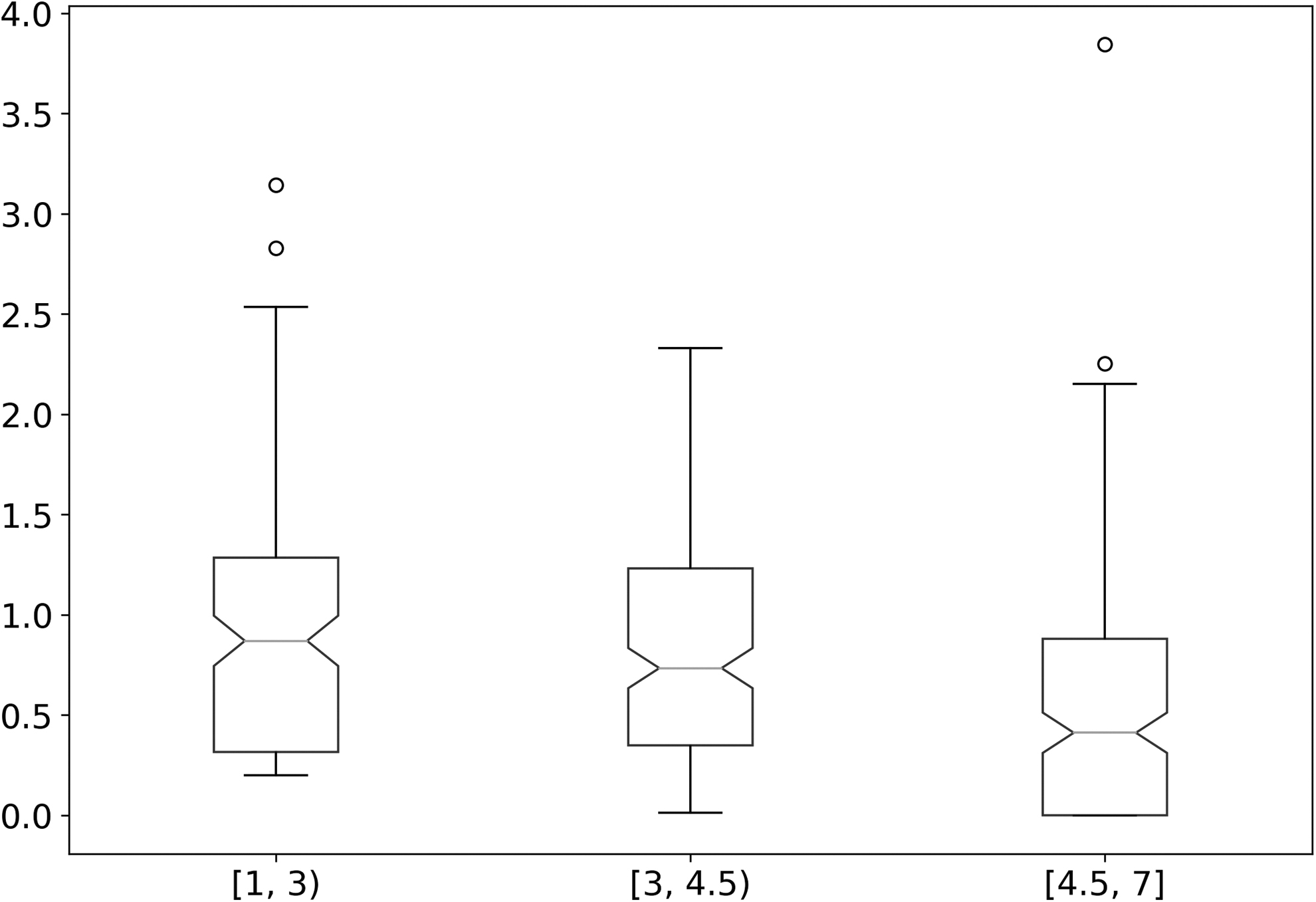
Box plot of the MADE by class of disability. MADE, mean absolute deviation error.

A longer tail can be detected, especially for patients with low disability level, suggesting a more difficult estimation in this range of EDSS. Conversely, a lower estimation error was obtained for the higher level of disability (EDSS of 4.5–7). Significant differences between EDSS groups were observed. Figure 3 depicts the error distribution by MS clinical phenotypes. Coherently with what is shown in Figure 2, a higher estimation error is observed for the early stage of the disease, namely the CIS group.

FIG. 3.

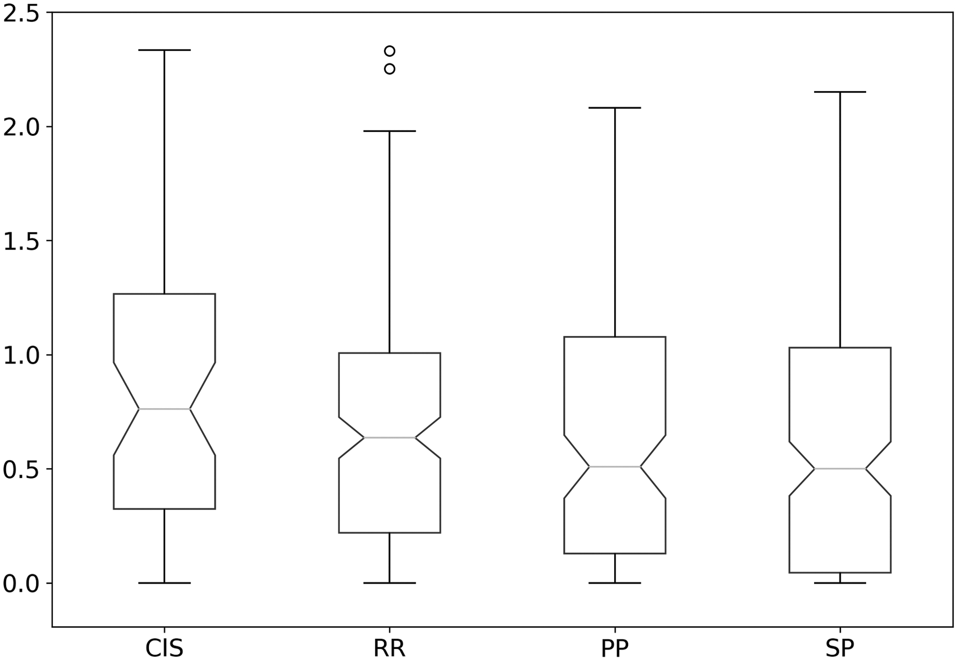
Box plot of the MADE by class of multiple sclerosis phenotypes.

Figure 4 depicts the average EDSS for the measured and estimated disability score obtained from the stacking generalization model.

FIG. 4.

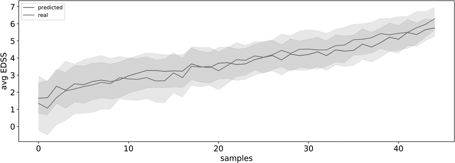
Comparison between measured (red) and estimated (blue) EDSS score. The two lines are obtained by, first, sorting the measured and estimated EDSS scores with respect to the test set for each of the 10 folds of the cross-validation. Then, for each sample, the average measured and estimated scores are computed obtaining an average measured and estimated distribution.

The two lines were obtained by computing the average measured and estimated scores by sorting them with respect to the holdout set for each of the 10 folds of the cross-validation. In Figure 4, we can notice that the two averaged (and standard deviations) curves (measured and estimated) are overlapping.

Model interpretability

The stacking generalization model was completed by an interpretability model to provide global and local explanations of the estimation process. Figure 5 reports the exponential increase of the cumulative relative importance of brain connections, while the red line defines the imposed threshold.

FIG. 5.

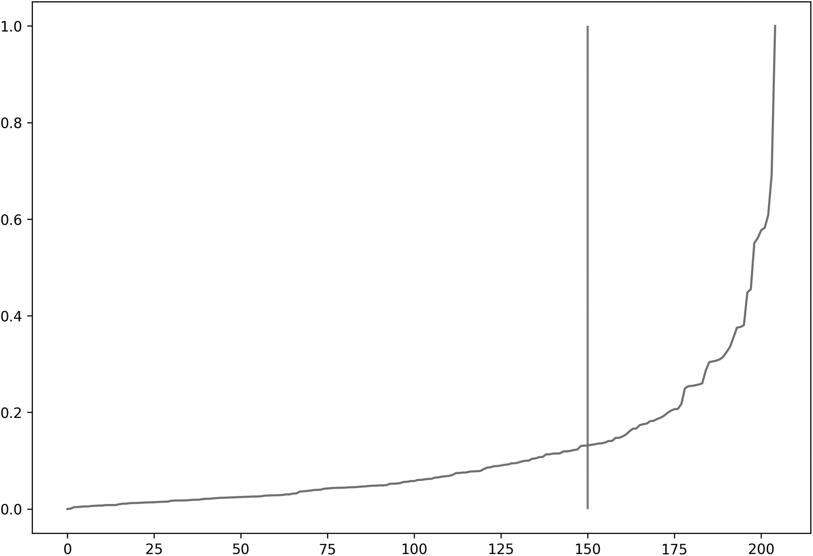
Global interpretability: sorted relative importance of brain connections expressed by indexed (idx) edges for readability purpose.

First, the global interpretability helped to identify brain connections playing an important role in disability estimation. These connections included frontal, temporal, and parietal cortical GM regions as well as subcortical GM regions. In particular, the highest number of connections corresponded to frontal/frontal, frontal/parietal, temporal/temporal, and temporal/parietal links. A visual representation of these connections is shown in Figure 6.

FIG. 6.

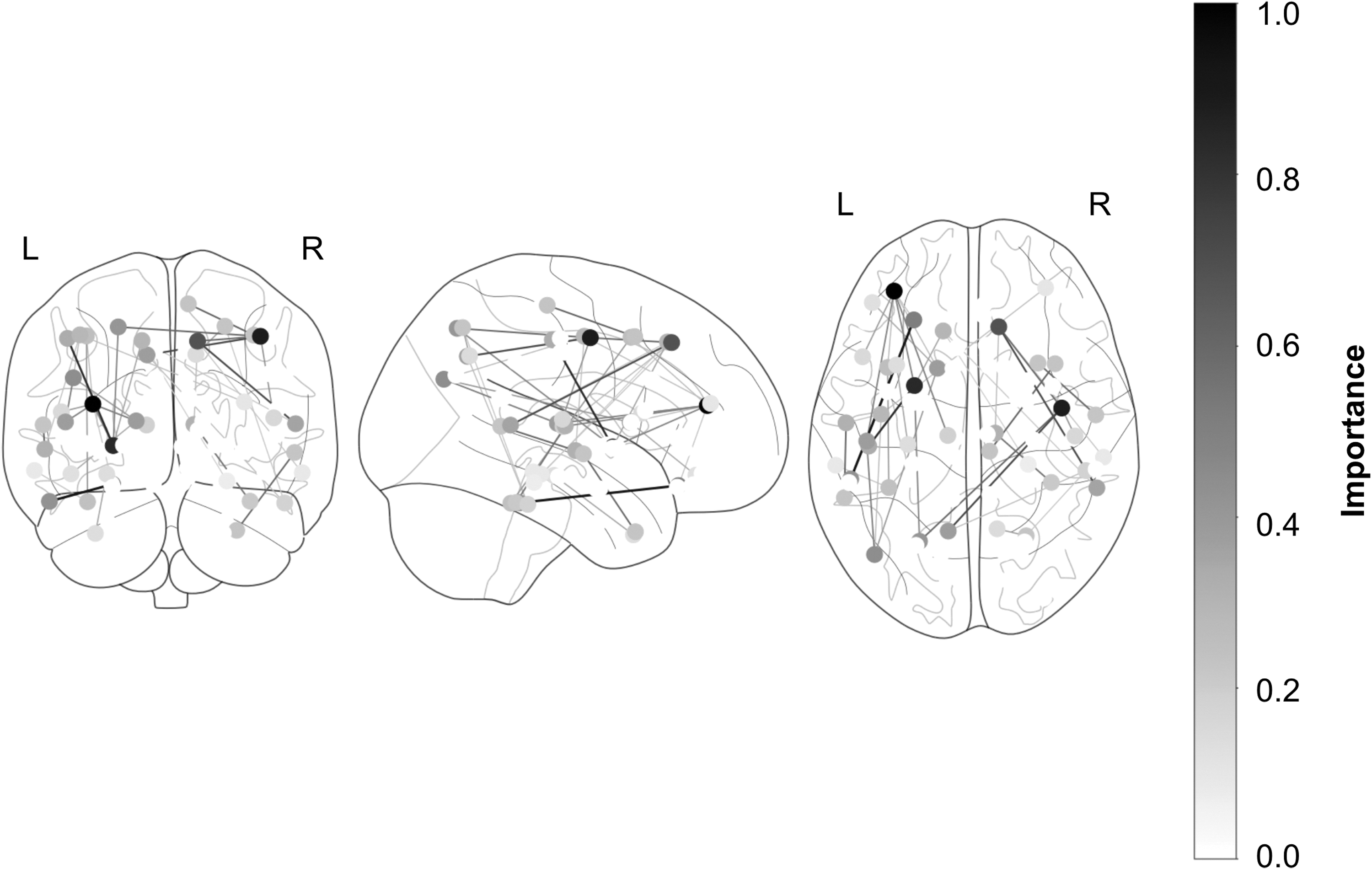
Global interpretability. Connectome representation of the most important edges for EDSS estimation. Nodes with high importance are depicted in a dark, while nodes with lower importance are depicted in white gray. The thickness of the connections lines represents edge importance.

Second, local interpretability was analyzed based on disability levels. Links with importance higher than the 95th percentile threshold were selected for visual purposes (Table 4). The left bank superior temporal sulcus represented the most important connection for the EDSS estimation in all of the three disability classes. Considering a threshold of importance of 0.5, in two EDSS classes (low and medium) out of the three, numerous WM links between GM regions were highlighted, including the left bank superior temporal sulcus with the left posterior cingulate and the right precuneus, confirming the importance of these connections for disability-level discrimination.

Table 4.

Brain Area Connection Importance by Class of Disability

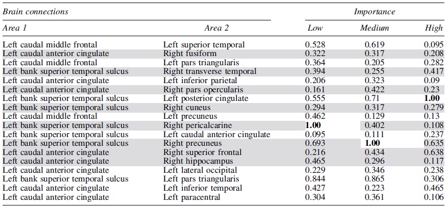
Most Important Brain Connections and Relative Importance for Three Classes of Expanded Disability Status Scale Score: Low ([1–3]), Medium ([3–4.5]), and High ([4.5–7]). In gray, the interhemispheric connections are highlighted, while in bold, the reference maximal scores of importance are emphasized.

To better characterize the connections playing an important role in the estimation process, the average number of WM fibers was calculated (Table 5) and the number of fibers participating in the estimation of each disability level was compared. Thirteen out of 19 connections resulted to be significantly different, pointing to a severe reduction in fibers' number in relation to an increased level of disability. This finding confirmed that the axonal neurodegeneration measured by DTI is directly related to the disability progression. For this reason, the ANOVA statistical test of hypothesis was repeated considering all connections for a baseline comparison. Only 10% and 7% of the total WM fibers resulted statistically significant at a 5% and 1% confidence level, respectively, confirming that the model focused on the most damaged WM fibers for estimating disability.

Table 5.

Brain Area Number of Connections by Class of Disability

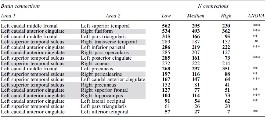
Mean number of white matter fiber connections for the 95th percentile most important edges divided into three classes of EDSS score: low ([1–3]), medium ([3-4.5]), and high ([4.5–7]). In gray, the interhemispheric connections are highlighted, while in bold, statistically significant deteriorations are emphasized by means of one-way ANOVA test of hypothesis (^*10%, ^**5%, ^***1% confidence level).

Finally, two observations are highlighted in Tables 4 and 5. First, by considering the 95th percentile of the most important brain connections, 78% are localized in the left hemisphere. Second, interhemispheric connectivity is well represented, amounting to 45% over the total connectivity. For comparison, the overall percentage average of interhemispheric connections, calculated over all the MS patients, amounts to 14%.

Discussion

MS is a neurological disease for which symptoms and severity can vary widely from patient to patient and progress at different rates. While the progression is rather slow and variable in RRMS patients, PPMS and SPMS patients are subjected to a progressive increase of disability, starting from the onset or later, respectively. To investigate the relationship between brain connectivity and disability, an ensemble of boosting methods was developed to estimate EDSS.

First, our method provided excellent performances (RMSE 0.9 ± 0.09) and outperformed the results obtained previously by Marzullo et al. (2019b), for which a convolutional neural network was considered (RMSE 1.08 ± 0.09).

Second, these findings demonstrated that DTI-based structural connectivity data represent an interesting alternative for disability estimation to conventional data including conventional MRI measures, such as the lesion load or tissue atrophy, with patient information such as age, gender, and disease duration. Indeed, it is known that lesion load is moderately correlated with the clinical status of the patient (Barkhof, 2002). For the characterization of microstructural WM alterations in MS patients, DTI is known to be more sensitive than conventional MRI as well as other patient information. Thus, the rapid technical improvements of MRI should facilitate the clinical accessibility of DTI acquisition, which is more cumbersome to realize in clinical routine.

Third, when observing the error distribution, a clear difference in performance, between low and high disability status, was found (F-score: 19.54). This is expected since higher levels of disability correspond to more degenerated WM fiber links, which are easily detectable by the model, based on the sensitivity of the DTI-based structural connectome. Also, the evaluation of low EDSS values is known to be cumbersome (Ebers, 2006) due to the highly variable clinical symptoms, which results in less accuracy. Indeed, a minimum of 1.0 U difference in EDSS is needed to define a significant clinical change (Goldman et al., 2010). Thus, automated ML methods may overcome this limitation by providing a more reliable estimation of disability based on the sensitivity of brain structural connectivity data. Moreover, by appropriately customizing the loss function to be optimized by the meta-learning model, the skewness of the EDSS can be taken into account and the optimization focus might be shifted toward lower scores. Indeed, the comparison between the holdout test estimation and the true EDSS score provided a visual evaluation of the goodness of fit, with standard deviations overlapping in most of the EDSS ranges (Fig. 4). This observation confirmed that our model was able to reach a high level of performance along the entire estimation range. Notwithstanding, the proposed approach is not intended to replace the current practice but rather to provide an additional tool for the neurologist to perform a more precise evaluation of a patient's status.

On top of the stacking ensemble model, our approach provided a global and local interpretability model to better identify the brain WM connections leading to predictive model performance. The global analysis highlighted the importance of large WM connections linking the frontal, temporal, and parietal GM regions. In particular, brain links between the frontal/frontal, frontal/parietal, temporal/temporal, and temporal/parietal GM regions correlate with the main brain networks usually damaged in MS patients (Andica et al., 2019; Bonavita et al., 2013; Han et al., 2017) and confirmed the involvement of these areas in the WM degeneration of MS patients (Curral et al., 2012; He et al., 2009). In addition, these regions may be predictive for discriminating MS phenotypes, especially between RRMS and SPMS patients, which represents one of the most interesting and difficult tasks for the automatic classification of MS profiles. In fact, previous studies highlighted that both global and regional cortical atrophies were observed to be more prominent in the left hemisphere relative to the right hemisphere (Narayana et al., 2012). Moreover, reduced mean cortical thickness, particularly in the frontal and temporal regions, may be a predictor of epilepsy in RRMS patients (Calabrese et al., 2012). Also, a significant reduction in GM thickness was observed in progressive stages of the MS disease, particularly in the parietal and precentral cortex (Chen et al., 2004). These results are coherent with our findings since more than half of our patients followed a progressive course.

Aside from the global analysis, the local interpretation focused on the importance of certain links depending on the level of disability. The main fiber links implied are connecting the left banks of superior temporal sulcus and the left caudal anterior cingulate GM regions. Indeed, the left bank thickness has been found to correlate with cognitive performance and motor skills in MS patients (Achiron et al., 2013; Pan et al., 2001), and the thickness reduction of the anterior cingulate was associated with loss in verbal and figural fluency as well as with hypoenergetic cognitive functioning in MS patients (Geisseler et al., 2016; Parisi et al., 2014).

In summary, the local analysis demonstrated the importance of the left and interhemispheric connections for the disability estimation process, reflecting more severe damages in the left hemisphere (Preziosa et al., 2017). These findings are concordant with the hypothesis that brain hemispheres can have different susceptibilities to damage accumulation (Thompson et al., 2003), particularly the left hemisphere, which is dominant for both handedness and language functions. This finding was already observed in neurodegenerative diseases such as Alzheimer's (Filippi et al., 1995). The importance of interhemispheric connections for disability estimation confirmed also that the corpus callosum is significantly affected in MS (Evangelou et al., 2000; Ozturk et al., 2010).

Notwithstanding, this study has few limitations. First, on the methodological aspects, the connectome analysis was performed using the Desikan atlas, which provides a gross parcellation of brain GM. In fact, large areas of the GM are considered for parcellation, which limits the interpretability of our results to specific WM tracts. However, the use of a more detailed parcellation atlas such as Glaser atlas will significantly increase the dimensionality of the problem, providing a higher chance of overfitting the training set. To prevent such limit, one should increase the size of the data set and/or exploit some a priori knowledge to preselect the most important GM regions.

Second, inflammation and neurodegeneration mechanisms are known to occur differently among the MS clinical courses, inflammation being predominant in the early stages of the disease (CIS and RRMS), while neurodegeneration (axonal and neuronal loss) mainly affects progressive courses (PPMS and SPMS). Thus, the distinction between these two main pathological mechanisms of MS would be of great interest to better understand the relationship between brain connectivity and patient disability. However, the EDSS distribution of our MS patients, both early stages and progressive courses, was very skewed toward an EDSS score of 4, due to the inclusion criteria. Unfortunately, this limitation prevented us to further analyze the differences between these two classifications.

Third, the EDSS score is mainly reliant on physical disability and in particular lower limb function. Since the MS clinical population is in general heterogeneous, not all patients may present predominantly motor symptoms, but rather so-called soft symptoms, such as fatigue, cognitive decline, and mood/anxiety disturbance, in agreement with the most important connections detected in this study, linking GM areas involved in higher order cognitive rather than movement-related functions. Thus, the EDSS may not be an absolute reliable measure of disability for the whole population of patients with MS, especially those with mild severity (Meyer-Moock et al., 2014; Saccà et al., 2017). For this purpose, the multiple sclerosis functional composite (MSFC) score, which takes into account other functional and cognitive capacities, is also performed and might better reflect the global disability of MS patients, especially those with moderate symptoms. Notwithstanding, the EDSS score was considered in this work due to its greater use in clinical practice (Amato and Ponziani 1999). Finally, it is well known that the spinal cord lesions have a significant role in patient disability, and thus, the study of only brain data constitutes probably a partial analysis of the issue.

Conclusion

In this work, we demonstrated the capability of our model to reach a good level of performance for disability estimation using DTI-based connectome data. To better understand the model decision pathway and identify its neural basis, a counterfactual model was implemented considering three levels of disability. A clear left hemispheric lateralization of WM fiber link degeneration, as well as interhemispheric connections, such as the corpus callosum, was detected and deemed to be relevant by our interpretability model along with frontal, temporal, and parietal GM regions.

As future work, we plan to extend the model by incorporating morphometric GM features and repeat the analysis considering other disability scales such as the MSFC score. Finally, we aim to extend this work by applying our model directly on large WM fiber bundles to precisely pin down the WM connections directly involved in the MS disability process.

Footnotes

Authors' Contributions

B.B. performed the analysis and wrote the article. A.M., C.S., and D.S.-M. supervised the writing of the article. C.S. performed the preprocessing. D.S.-M. and F.D.-D. coordinated the study and performed the data acquisitions.

Author Disclosure Statement

No competing financial interests exist.

Funding Information

This study is funded by the following projects: European Research Council within the grant 813120-2018 of Marie Skłodowska-Curie Innovative Training Networks (ITN) of the Horizon 2020 through the INSPiRE-MED project. French National Research Agency (ANR) within the national program “Investissements d'Avenir” through the OFSEP project (ANR-10-COHO-002).

References

Achiron

, Chapman

, Tal

, et al. 2013. Superior temporal gyrus thickness correlates with cognitive performance in multiple sclerosis. Brain Struct Funct, 218:943–950.

Amato

, Ponziani

. 1999. Quantification of impairment in MS: discussion of the scales in use. Multiple Sclerosis, 5:216–219.

Andica

, Hagiwara

, Kamagata

, et al. 2019. Gray matter alterations in early and late relapsing-remitting multiple sclerosis evaluated with synthetic quantitative magnetic resonance imaging. Sci Rep, 9:8147.

Bakshi

, Thompson

, Rocca

, et al. 2008. MRI in multiple sclerosis: current status and future prospects. Lancet Neurol, 7:615–625.

Barkhof

2002. The clinico-radiological paradox in multiple sclerosis revisited. Curr Opin Neurol, 15:239–245.

Basser

, Pajevic

, Pierpaoli

, et al. 2000. In vivo fiber tractography using DT-MRI data. Magnet Reson Med, 44:625–632.

Bonavita

, Tedeschi

, Gallo

. 2013. Morphostructural MRI abnormalities related to neuropsychiatric disorders associated to multiple sclerosis. Mult Scler Int, 2013:102454.

Bushnik

2011. Expanded Disability Status Scale. Encyclop Clin Neuropsychol. 997–999.

Calabrese

, Grossi

, Favaretto

, et al. 2012. Cortical pathology in multiple sclerosis patients with epilepsy: a 3 years longitudinal study. J Neurol Neurosurg Psychiatry, 83:49–54.

10.

Chen

, Guestrin

Xgboost: a scalable tree boosting system. In 22nd ACM SIGKDD International Conference on Knowledge Discovery and Data Mining, Association for Computing Machinery, New York, USA, 2016, pp. 785–794.

11.

Chen

, Narayanan

, Collins

, et al. 2004. Relating neocortical pathology to disability progression in multiple sclerosis using MRI. Neuroimage, 23:1168–1175.

12.

Curral

, Correia

, Lopes

, et al. 2012. Dementia in multiple sclerosis: report of a case with cortical gray matter involvement and frontotemporal-like clinical features. Psychiatry, 202:172–174.

13.

Declan

, Trip

. 2017. Resolving the clinic-radiological paradox in multiple sclerosis. F1000Res, 6:1828.

14.

Desikan

, Ségonne

, Fischl

, et al. 2006. An automated labeling system for subdividing the human cerebral cortex on MRI scans into gyral based regions of interest. Neuroimage, 31:968–980.

15.

Ebers

GC.

2006. Disease evolution in multiple sclerosis. J Neurol, 253:vi3–vi8.

16.

Evangelou

, Konz

, Esiri

, et al. 2000. Regional axonal loss in the corpus callosum correlates with cerebral white matter lesion volume and distribution in multiple sclerosis. Brain, 123:1845–1849.

17.

Filippi

, Martino

, Mammi

, et al. 1995. Does hemispheric dominance influence brain lesion distribution in multiple sclerosis?. J Neurol Neurosurg Psychiatr, 58:748–749.

18.

Friedman

JH.

2001. Greedy function approximation: a gradient boosting machine. Ann Statist, 5:1189–1232.

19.

Geisseler

, Pflugshaupt

, Bezzola

, et al. 2016. Cortical thinning in the anterior cingulate cortex predicts multiple sclerosis patients' fluency performance in a lateralised manner. Neuroimage Clin, 10:89–95.

20.

Ghasemi

, Razavi

, Nikzad

. 2016. Multiple sclerosis: pathogenesis, symptoms, diagnoses and cell-based therapy. Cell J, 19:1–10.

21.

Gilpin

, Bau

, Yuan

, et al. 2018. Explaining explanations: an overview of interpretability of machine learning. Sci Adv Anal (DSAA), 80–89.

22.

Goldman

, Motl

, Rudick

. 2010. Possible clinical outcome measures for clinical trials in patients with multiple sclerosis. Therap Adv Neurol Disord, 3:229–239.

23.

Goodin

DS.

2014. The epidemiology of multiple sclerosis: insights to disease pathogenesis. Handb Clin Neurol, 122:231–266.

24.

Guo

, Nejati

, Cheung

. Deep neural networks on graph signals for brain imaging analysis. In IEEE International Conference on Image Processing (ICIP), Beijing, China, 2017, pp. 3295–3299.

25.

Han

, Tian

, Han

, et al. 2017. Correlation between white matter damage and gray matter lesions in multiple sclerosis patients. Neural Regen Res, 12:787–794.

26.

Hastie

, Tibshirani

, Friedman

. 2009. The Elements of Statistical Learning. New York, NY: Springer.

27.

, Dagher

, Chen

, et al. 2009. Impaired small-world efficiency in structural cortical networks in multiple sclerosis associated with white matter lesion load. Brain, 132:3366–3379.

28.

Jain

, Sima

, Ribbens

, et al. 2015. Automatic segmentation and volumetry of multiple sclerosis brain lesions from MR images. Neuroimage, 8:367–375.

29.

Jenkinson

, Beckmann

, Behrens

TEJ

, et al. 2012. FSL. Neuroimage, 62:782–790.

30.

Jütten

, Mainz

, Gauggel

, et al. 2019. Diffusion tensor imaging reveals microstructural heterogeneity of normal-appearing white matter and related cognitive dysfunction in glioma patients. Front Oncol, 9:536.

31.

, Meng

, Finley

, et al. 2017. LightGBM: a highly efficient gradient boosting decision tree. Adv Neural Inform Process Syst, 30:3146–3154.

32.

Kocevar

, Stamile

, Hannoun

, et al. 2016. Graph theory-based brain connectivity for automatic classification of multiple sclerosis clinical courses. Front Neurosci, 10:478.

33.

Kolcava

, Kocica

, Hulova

, et al. 2020. Conversion of clinically isolated syndrome to multiple sclerosis: a prospective study. Mult Scler Relat Disord, 44:102262.

34.

Kotu

2015. Predictive Analytics and Data Mining. Journals and Books. Amsterdam: Morgan Kaufmann Publishing and Elsevier, pp. 17–36.

35.

Kurtzke

JF.

1983. Rating neurologic impairment in multiple sclerosis: an expanded disability status scale (EDSS). Neurology, 33:1444–1452.

36.

Kuvalekar

, Kamath

, Ashok

, et al. 2015. Quality of life among persons with physical disability in Udupi Taluk: a cross sectional study. J Fam Med Prim Care, 4:69–73.

37.

Law

, Traboulsee

, Li

, et al. 2019. Machine learning in secondary progressive multiple sclerosis: an improved predictive model for short-term disability progression. Mult Scler J Exp Transl Clin, 5:2055217319885983.

38.

Liu

, Cui

, Jiang

, et al. 2004. A combinational feature selection and ensemble neural network method for classification of gene expression data. BMC Bioinformatics, 5:136.

39.

Lublin

, Reingold

, Cohen

. 2014. Defining the clinical course of multiple sclerosis. Neurology, 83:278–286.

40.

Lynch

, Parmenter

, Denney

. 2005. The association between cognitive impairment and physical disability in multiple sclerosis. Mult Scler, 11:469–476.

41.

Marzullo

, Kocevar

, Stamile

, et al. 2019a. Classification of multiple sclerosis clinical profiles via graph convolutional neural networks. Front Neurosci, 13:594.

42.

Marzullo

, Kocevar

, Stamile

, et al. Prediction of multiple sclerosis patient disability from structural connectivity using convolutional neural networks. In Conference of the Proceedings of the IEEE Engineering in Medicine and Biology Society, Berlin, Germany, 2019b, pp. 2087–2090.

43.

McDonald

, Compston

, Edan

, et al. 2001. Recommended diagnostic criteria for multiple sclerosis: guidelines from the international panel on the diagnosis of multiple sclerosis. Ann Neurol, 50:121–127.

44.

Meyer-Moock

, Feng

, Maeurer

, et al. 2014 Systematic literature review and validity evaluation of the Expanded Disability Status Scale (EDSS) and the Multiple Sclerosis Functional Composite (MSFC) in patients with multiple sclerosis. BMC Neurol, 14:58.

45.

Narayana

, Govindarajan

, Goel

, et al. 2012. Regional cortical thickness in relapsing remitting multiple sclerosis: a multi-center study. Neuroimage Clin, 2:120–131.

46.

Ozturk

, Smith

, Gordon-Lipkin

, et al. 2010. MRI of the Corpus Callosum in multiple sclerosis: association with disability. Mult Scler, 16:166.

47.

Pan

, Krupp

, Elkins

, et al. 2001. Cognitive dysfunction lateralizes with NAA in multiple sclerosis. Appl Neuropsychol, 8:155–160.

48.

Parisi

, Rocca

, Valsasina

, et al. 2014. Cognitive rehabilitation correlates with the functional connectivity of the anterior cingulate cortex in patients with multiple sclerosis. Brain Imaging Behav, 8:387–393.

49.

Polman

, Reingold

, Banwell

, et al. 2011. Diagnostic criteria for multiple sclerosis: 2010 revisions to the mcdonald criteria. Ann Neurol, 69:292–302.

50.

Preziosa

, Pagani

, Mesaros

, et al. 2017. Progression of regional atrophy in the left hemisphere contributes to clinical and cognitive deterioration in multiple sclerosis: a 5-year study. Hum Brain Mapp, 38:5648–5665.

51.

Reuter

, Schmansky

, Rosas

, et al. 2012. Within-subject template estimation for unbiased longitudinal image analysis. Neuroimage, 61:1402–1418.

52.

Saccà

, Costabile

, Carotenuto

, et al. 2017. The EDSS integration with the Brief International Cognitive Assessment for Multiple Sclerosis and orientation tests. Mult Scler J, 23:1289–1296.

53.

Smith

, Tournier

, Calamante

, et al. 2012. Anatomically-constrained tractography: improved diffusion MRI streamlines tractography through effective use of anatomical information. Neuroimage, 62:1924–1938.

54.

Thompson

, Hayashi

, Zubicaray

, et al. 2003. Dynamics of gray matter loss in alzheimer's disease. Neuroscience, 23:994–1005.

55.

Tournier

, Calamante

, Connelly

, et al. 2012. MRtrix: diffusion tractography in crossing fiber regions. Int J Imaging Syst Technol, 22:53–66.

56.

Tousignant

, Lemâıtre

, Precup

, et al. Prediction of disease progression in multiple sclerosis patients using deep learning analysis of MRI data. In Proceedings of The 2nd International Conference on Medical Imaging with Deep Learning, PMLR, London, England, 2019, 102:483–492.

57.

Traboulsee

, Li

, Zhao

, et al. 2005. Conventional MRI techniques in multiple sclerosis. MR Imaging in White Matter Diseases of the Brain and Spinal Cord. Berlin Heidelberg: Springer, pp. 211–223.

58.

Tsoumakas

, Vlahavas

Random k-label sets: an ensemble method for multilabel classification. In Proceedings of the 18th European Conference on Machine Learning, Springer, Warsaw, Poland, 2007, pp. 406–417.

59.

Van Munster

CEP

, Uitdehaag

BMJ

. 2017. Outcome measures in clinical trials for multiple sclerosis. CNS Drugs, 31:217–236.

60.

Veronika

, Ershov

, Gulin

. 2018. CatBoost: gradient boosting with categorical features support, arXiv:1810.11363.

61.

Washimkar

, Chede

. Application of FCM clustering on AM-FM to detect MRI disease progression for multiple sclerosis. In International Conference on Computational Intelligence and Commutation Networks (CICN), IEEE, Jabalpur, India, 2015, pp. 283–287.

62.

Witten

, Eibe

. 2020. Data Mining: Practical Machine Learning Tools and Techniques. Journals and Books. Amsterdam: Morgan Kaufmann Publishing and Elsevier.

63.

Wolpert

DH.

1992. Stacked generalization. Neural Netw, 5:241–259.

64.

Yong

, Alan

. 2010. Graph theoretical modelling of brain connectivity. Curr Opin Neurol, 23:341–350.

65.

Zhao

, Healy

, Rotstein

, et al. 2017. Exploration of machine learning techniques in predicting multiple sclerosis disease course. PLoS One, 12:e0174866.