A Wavelet-Based Approach for Estimating Time-Varying Connectivity in Resting-State Functional Magnetic Resonance Imaging

Abstract

Introduction:

The selection of an appropriate window size, window function, and functional connectivity (FC) metric in the sliding window method is not straightforward due to the absence of ground truth.

Methods:

A previously proposed wavelet-based method was accordingly adjusted for estimating time-varying FC (TVFC) and was applied to a large high-quality, low-motion dataset of 400 resting-state functional magnetic resonance imaging data. Specifically, the wavelet coherence magnitude and relative phase were averaged across wavelet (frequency) scales to yield TVFC and synchronization patterns. To assess whether the observed fluctuations in TVFC were statistically significant (dynamic FC [dFC]; the distinction between TVFC and dFC is intentional), surrogate data were generated using the multivariate phase randomization (MVPR) and multivariate autoregressive randomization (MVAR) methods to define the null hypothesis of dFC absence.

Results:

By averaging across all frequencies, core regions of the default mode network (DMN; medial prefrontal and posterior cingulate cortices, inferior parietal lobes, hippocampal formation) were found to exhibit dFC (test–retest reproducibility of 90%) and were also synchronized in activity (−15° ≤ phase ≤15°). When averaging across distinct frequency bands, the same dynamic connections were identified, with the majority of them identified in the frequency range (0.01, 0.198) Hz, though with lower test–retest reproducibility (<66%). Additional analysis suggested that MVPR method better preserved properties (p < 10⁻¹⁰), including time-averaged coherence, of the original data compared with MVAR approach.

Conclusions:

The wavelet-based approach identified dynamic associations between the core DMN regions with fewer choices in parameters, compared with sliding window method.

Impact statement

We employed a wavelet-based method, previously used in the literature, and proposed modifications to assess time-varying functional connectivity in resting-state functional magnetic resonance imaging. With this approach, dynamic connections within the default mode network were identified, involving the medial prefrontal and posterior cingulate cortices, inferior parietal lobes, and hippocampal formation, which were also highly consistent in test–retest analysis (test–retest reproducibility of 90%), without the need to select window size, window function, and functional connectivity metric as with the sliding window method, whereby no consensus on the appropriate choices of hyperparameters currently exists in the literature.

Introduction

Functional connectivity (FC) is an integral part of resting-state functional magnetic resonance imaging (rs-fMRI) data analysis, and it has been suggested that it varies during the scanning session, with the estimation of time-varying FC (TVFC) being performed in the time domain or through a joint representation in the time–frequency domain (Hutchison et al., 2013a; Lurie et al., 2020, Preti et al., 2017). Time domain methodologies include the identification of recurring spatiotemporal patterns (Majeed et al., 2011), the detection of coactivation patterns (Liu and Duyn, 2013), the application of temporal Independent Component Analysis (Smith et al., 2012), as well as the common sliding window approach (Hutchison et al., 2013a, Savva et al., 2019), while time–frequency domain approaches have been used on a more limited basis (Preti et al., 2017).

The sliding window method uses a window of predefined size and shape that is progressively shifted over the rs-fMRI time series, estimating a chosen FC metric within each segment. Common choices of FC metrics include the Pearson linear correlation (Hutchison et al., 2013a, Preti et al., 2017) and the precision matrix (Varoquaux and Craddock, 2013). Window length is often determined using empirical evidence, with typical values ranging between 30 and 60 sec (Lurie et al., 2020; Preti et al., 2017), while larger values up to 240 sec have been also used (Chang and Glover, 2010; Hutchison et al., 2013b). Finally, the use of a window function other than the rectangular has been associated with the suppression of motion-related noise that likely remains in the data even after preprocessing (Lindquist et al., 2014; Preti et al., 2017).

On the contrary, representing rs-fMRI time series in the time–frequency domain aims at identifying dominant frequencies in TVFC along with their variation in time (Hramov et al., 2014; Preti et al., 2017). This approach was initially applied to rs-fMRI data in a previous study (Chang and Glover, 2010), who performed the TVFC analysis across multiple (frequency) scales by applying the wavelet transform to the entire time series. In the same study, time-varying statistical dependencies between brain regions were quantified using wavelet coherence (Grinsted et al., 2004; Torrence and Webster, 1999), which simultaneously allows the estimation of time-varying phase values between the examined time series.

This approach requires only the selection of a wavelet basis function, with the majority of rs-fMRI studies employing Morlet wavelets (Chang and Glover, 2010; Wang et al., 2017; Yaesoubi et al., 2015, 2017). Nevertheless, this comes at the cost of obtaining a representation with increased dimensionality (time and frequency); thus, limiting the applications of wavelets to TVFC up to date (Preti et al., 2017). Reduction of dimensionality was achieved by either estimating the time-averaged coherence (TAC) (Chang and Glover, 2010; Wang et al., 2017), or employing the k-means algorithm to summarize TVFC patterns across different frequency bands (Yaesoubi et al., 2015, 2017).

The aim of this study is to propose a wavelet-based method for assessing dynamic FC (dFC; statistically significant TVFC) requiring fewer choices in terms of hyperparameters, as compared with the sliding window approach, where no consensus on the choice of appropriate window size, window function, and FC metric currently exists (Preti et al., 2017; Savva et al., 2019, 2020). To this end, the method proposed in Chang and Glover (2010) was modified to measure temporal variability using the coherence magnitude (which can be viewed as correlation coefficient in the time–frequency domain), while relative phase was used to assess synchronization patterns.

In Chang and Glover (2010), temporal variability was assessed by incorporating coherence magnitude and relative phase into a single complex quantity. By treating amplitude and phase independently, we aimed at assessing both dFC and synchronized activity patterns, while averaging over all frequency scales yielded more reproducible results compared with averaging over narrow bands. To assess dFC, a hypothesis testing framework was constructed based on surrogate data using the multivariate phase randomization (MVPR) and multivariate autoregressive randomization (MVAR) methods. In this context, we also systematically examined the extent to which these methods better preserve the properties of the original data, including TAC, which is shown to be preserved with the MVPR method for the first time to our knowledge.

The proposed method was used for detecting dFC patterns within the default mode network (DMN), since the DMN is perhaps the most widely studied resting-state network in both pathological and healthy conditions (Andrews-Hanna et al., 2010; Buckner et al., 2008; Damoiseaux et al., 2006; Raichle et al., 2001). Moreover, in the absence of an unequivocal ground truth in rs-fMRI (Shakil et al., 2016) we considered several sessions to assess reproducibility, and the fact that previous studies identified dynamic connections within DMN (Chang and Glover, 2010; Savva et al., 2019; Zalesky et al., 2014), focusing on the DMN facilitated comparison of results with previous work.

Materials and Methods

Data acquisition and preprocessing

Two hundred low-motion rs-fMRI datasets from healthy individuals were acquired from human connectome project (HCP), S900 release (Van Essen et al., 2013). A detailed description of the data acquisition protocol and preprocessing can be found in previous studies (Glasser et al., 2013; Van Essen et al., 2013). In brief, the fMRI data were acquired using a customized 3T Siemens scanner with gradient echo planar imaging, repetition time (TR) = 720 msec (1200 volumes in total), TE = 33.1 msec, flip angle = 52°, field of view = 208 × 180 mm², reconstruction matrix = 104 × 90, voxel dimensions = 2 × 2 × 2 mm³, multiband factor of 8, echo spacing = 0.58 msec, and bandwidth = 2290 Hz/Px.

In this study, datasets from the first session (left-right [LR] and right-left [RL] encoding) were considered to perform a test–retest analysis (for each subject one dataset was acquired with LR and one with RL encoding). Moreover, the low-motion data were defined as those for which the mean framewise displacement (FD) was <0.2 mm in both scanning sessions (Power et al., 2012). Data were provided by the Human Connectome Project, WU-Minn Consortium (Principal Investigators: David Van Essen and Kamil Ugurbil; 1U54MH091657) funded by the 16 NIH Institutes and Centers that support the NIH Blueprint for Neuroscience Research; and by the McDonnell Center for Systems Neuroscience at Washington University.

We used data preprocessed with the minimal pipeline, consisting of removal of spatial distortions due to gradient fields' nonlinearities, head motion correction, distortion correction due to B0 field, alignment to the T1-weighted structural image, and nonlinear alignment to the 2 mm Montreal Neurological Institute space (Glasser et al., 2013). For reducing blurring effects, the aforementioned transformations were applied to the raw data in a single step using spline interpolation. A global intensity normalization to the value of 10,000 and smoothing using a 2 mm full width at half maximum geodesic Gaussian procedure were also performed. Finally, a high-pass temporal filtering step (cutoff time of 150 sec) was applied for suppressing slow drifts and trends (Savva et al., 2019; Smith et al., 2013).

Time-series extraction

Regions of interest (ROIs) were defined following previous studies (Savva et al., 2019, 2020), using functional masks of Dorsal and Ventral DMN acquired from Stanford University Functional Imaging in Neuropyschiatric Disorders Lab (available online). (Shirer et al., 2012). All ROIs are mentioned in Table 1 along with coordinates of their region centroids and their abbreviations. To extract time series representing the blood oxygen level dependent (BOLD) time series of each ROI, the mean across all voxels was calculated. This procedure was applied to all 200 subjects for both test and retest datasets, resulting in 13 time series for each subject and each dataset.

Table 1.

Regions of Interest Comprising the Default Mode Network Employed in this Study

ROI	Coordinates (x, y, z)	Abbreviation
Cerebellum	(14, −46, −52)	Cer
Left hippocampus	(−24, −30, −14)	L-Hipp
Right hippocampus	(26, −24, −16)	R-Hipp
Medial prefrontal cortex	(0, 52, 14)	mPFC
Thalamus	(0, −10, 6)	Thal
Posterior cingulate cortex	(0, −54, 30)	PCC
Right inferior parietal	(44, −72, 32)	R-IP
Left inferior parietal	(−36, −80, 32)	L-IP
Left inferior parietal—2	(−48, −66, 34)	L-IP(2)
Anterior cingulate gyrus	(0, −14, 36)	ACG
Right middle frontal gyrus	(28, 32, 44)	R-MFG
Precuneus	(0, −56, 56)	Prec
Left middle frontal gyrus	(−26, 14, 52)	L-MFG

Coordinates are in the MNI space.

MNI, Montreal Neurological Institute; ROI, regions of interest.

Surrogate data

Surrogate data were generated using the available time series, aiming to produce data that are characterized by dFC absence (Hindriks et al., 2016) also maintaining basic properties of the original data, such as cross- and autocorrelation, cross- and power spectral density, as well as amplitude distribution (Savva et al., 2019; Zalesky et al., 2014). In this study, the MVPR method was employed and compared with the MVAR approach, in terms of both the identified dynamic connections and property preservation of the original data. The multivariate version of both methods was selected instead of the bivariate alternative, since the latter has been associated with a large number of false positives (Liegeois et al., 2017). Both methods are described in the Supplementary Data (Section S1).

Wavelet analysis

Wavelet transform coherence

Let x (n) be a discrete sequence representing the BOLD response from a brain region. The continuous wavelet transform of x (n) is defined as follows:

where s denotes the wavelet scale, △t = TR is the time step, and ψ₀ is the wavelet basis function. In this study, the Morlet wavelet basis was chosen (Chang and Glover, 2010; Yaesoubi et al., 2015, 2017).

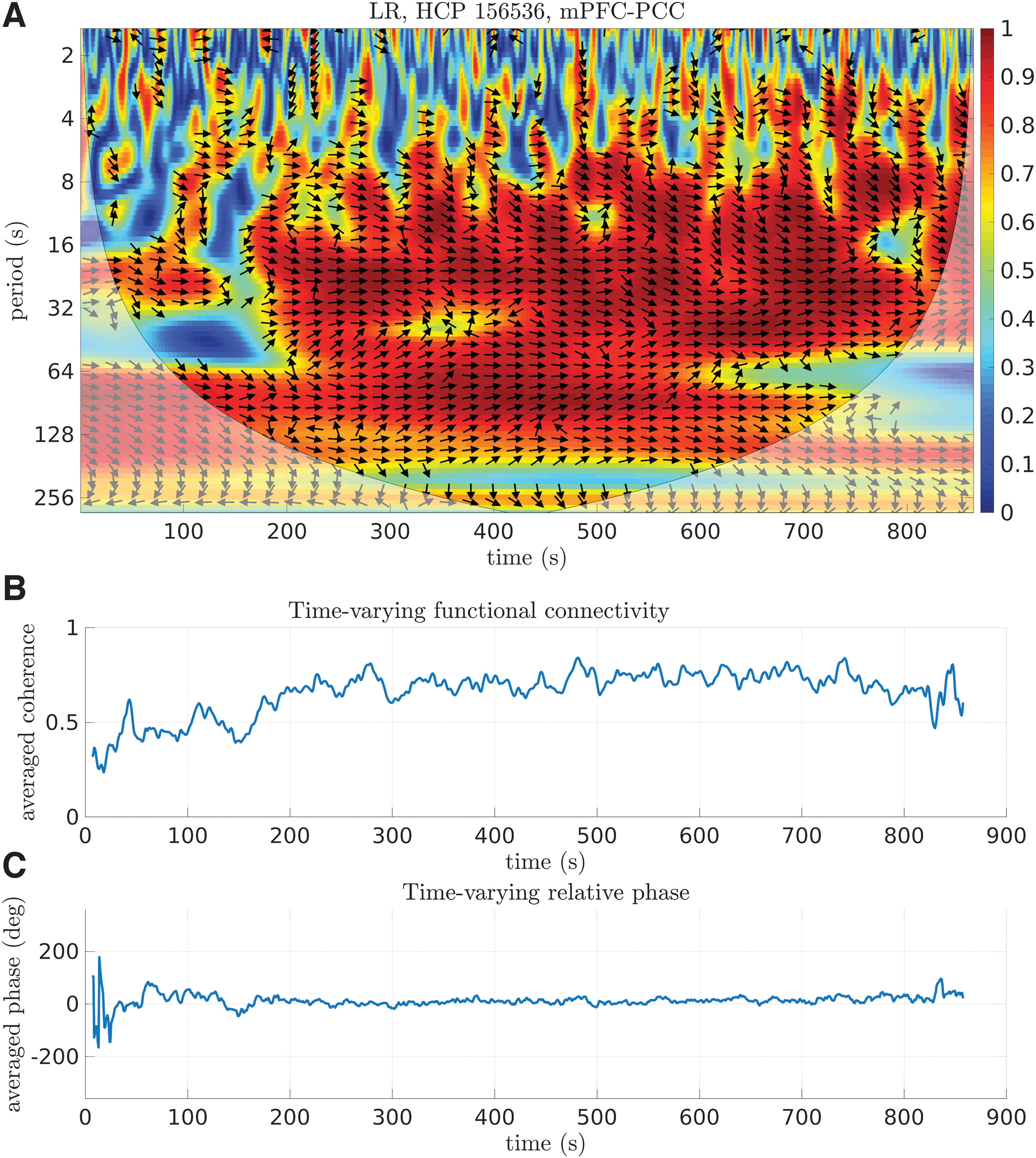
Subsequently, all wavelet transforms of the time series were combined in a pairwise manner to estimate the cross-wavelet transform as follows: W^XY (n, s) = W^X (n, s) W^Y* (n, s), where W^Y* denotes the complex conjugate of W^Y . From the cross-wavelet transform, the cross-wavelet power $|W^{X Y} (t, s)|$ can be estimated expressing the shared power between signals X and Y in the time–frequency domain, as well as their relative phase: $Φ (n, s) = arg (W^{X Y} (n, s))$ (Chang and Glover, 2010). In addition, it is often useful to provide a normalized measure of coherency (which can be viewed as a correlation coefficient in the time–frequency domain) between the examined signals in terms of their wavelet transform similarity (Grinsted et al., 2004; Torrence and Webster, 1999). To this end, the wavelet transform coherence (WTC; Fig. 1A) is defined as follows:

FIG. 1.

Representative example of WTC, TVFC, and time-varying relative phase. (A) WTC and relative phase estimated from the mPFC–PCC time series from a representative subject (HCP 156536; mean FD = 0.076 mm; LR scanning session). Right pointing arrows indicate 0° relative phase, while upward pointing arrows denote relative phase of 90° (plotted for coherence values >0.5); (B) TVFC and (C) time-varying relative phase. For averaging coherence and phase in (B) and (C), respectively, values across all frequency scales and outside the COI (shaded area) were considered. COI, cone of influence; FD, framewise displacement; HCP, human connectome project; LR, left–right encoding; mPFC, medial prefrontal cortex; PCC, posterior cingulate cortex; TVFC, time-varying functional connectivity; WTC, wavelet transform coherence. Color images are available online.

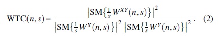
WTC ranges between 0 and 1, while SM indicates smoothing for both time and frequency scales (Chang and Glover, 2010; Grinsted et al., 2004).

Time-varying functional connectivity

To estimate TVFC, the average coherence across frequency scales (columns of the WTC spectrum) was computed yielding a new time series with fluctuating coherence values (Fig. 1B). The averaging procedure aimed at incorporating interaction effects from all frequency scales for quantifying statistical associations between the examined time series. Note that at the beginning and end of the time series relatively few values were averaged due to “Cone of Influence” (COI; Fig. 1A, shaded area), a region where edge effects occur due to limited duration of the time series; therefore, averaged coherence was calculated when >20 values were available. As a result, 18 values (9 from both ends) were discarded (a total of 12.96 sec) from further analysis.

TVFC was also estimated focusing on frequency bands defined previously (Di Martino et al., 2008; Zuo et al., 2010): slow-2 (0.198 Hz<f ≤ 0.69 Hz; 1.45 sec ≤ scale <5.1 sec), slow-3 (0.073 Hz < f ≤ 0.198 Hz; 5.1 sec ≤ scale <13.7 sec), slow-4 (0.027 Hz < f ≤ 0.073 Hz; 13.7 sec ≤ scale <37 sec), slow-5 (0.01 Hz < f ≤ 0.027 Hz; 37 sec ≤ scale <100 sec), and slow-6 (f ≤ 0.01 Hz; scale ≥100 sec). In this case, due to the segregation of the time–frequency domain and the presence of COI especially in the slowest frequencies, the averaged coherence within each frequency band was estimated when >5 values were available; hence, 4, 14, 36, 96, and 256 values from both ends were discarded for the slow-2, slow-3, slow-4, slow-5, and slow-6 bands, respectively.

Time-varying relative phase

Wavelet analysis also facilitates the estimation of relative phase between each pair of signals by estimating arg(W^XY (n, s)). In this context, a new time series can be obtained by averaging phase values across frequency scales, similar to TVFC, indicating the time-varying patterns of relative phase (TVRP) between the examined region pairs. Note that the average was estimated using the circular mean defined as (Berens, 2009; Jammalamadaka and Sengupta, 2001) follows:

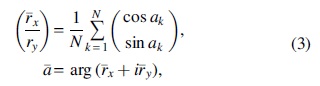
where a_k represents phase values and $i = \sqrt{- 1}$ .

From Eq. (3), the length of the average resultant vector can be estimated as

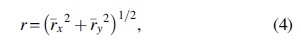
quantifying the concentration of the data around the average direction (circular spread; Berens, 2009). A value closer to unity indicates greater concentration around the mean direction. As in the case of TVFC, 9 values were discarded from both ends of TVRP. From a representative example (Fig. 1C), it can be seen that TVRP ranges between around −200° and 200° during the first minute of the scanning session, indicating potential desynchronization patterns before settling to a value of ∼0° for the remainder of the scanning session, while for other subjects (Supplementary Fig. S1 in the Supplementary Data), the corresponding TVRP was ∼0° for the entire scanning session. As in the case of TVFC, TVRP was also estimated by using phase values within the previously defined frequency bands.

Time-averaged coherence

Apart from averaging across frequency scales as described above, averaging across time (TAC) can be performed (Chang and Glover, 2010). In this study, TAC was considered as an additional property of the original time series that must be preserved during surrogate data generation (for the first time to our knowledge). To incorporate both WTC and the relative phase into a single representation, Chang and Glover (2010) suggested estimating TAC to identify peaks of the average-across-time coherence. Specifically, TAC (Fig. 2) was calculated within four equally spaced phase intervals as shown in Eq. (5):

FIG. 2.

TAC. Thresholded WTC at the 95th percentile (left) and TAC curves (right) within each phase interval for a representative low-motion subject (HCP 156536; mean FD = 0.076 mm; LR dataset). The highest coherence between mPFC and PCC regions was observed for the phase interval 0 ± π/4 (blue curve in the right panel). TAC denotes the coherence distribution across the scanning session at different frequency scales relative to phase values. TAC, time-averaged coherence. Color images are available online.

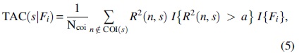
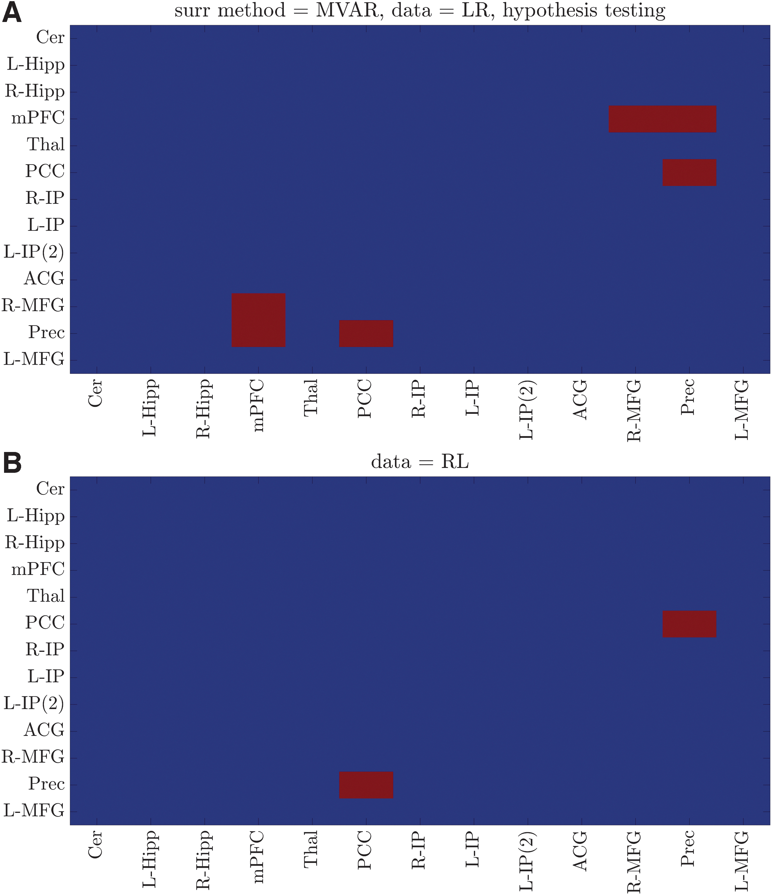
where i = 1, 2, 3, 4, I is the indicator function resulting in a value of 1 when the condition inside the curly brackets is true and zero otherwise, and a is a threshold denoting the highest coherence values. Here, a was set as the 95th percentile of WTC(n, s). Moreover, F_i denotes the set of phase values belonging to a particular range as indicated below:

Finally, a normalization was applied by dividing with N _coi, which is the total number of points outside the COI.

Hypothesis testing

To assess whether the observed fluctuations in TVFC were statistically significant, the variance $(σ^{2})$ of the TVFC time series was estimated for both the original $(σ_{o r i g i n a l}^{2})$ and surrogate data. In the case of surrogate data, this step produced a total of 250 variance values (null distribution) for each region pair and each subject. Following previous studies, these $(\begin{matrix} 13 \\ 2 \end{matrix}) = 78$ null distributions were aggregated into a single distribution with a larger number of samples; that is, 78 × 250 = 19500 (Savva et al., 2019; Zalesky et al., 2014). In addition, for both original and surrogate data, the average-across-subjects variance was estimated to conduct analysis at the group level (Hindriks et al., 2016; Savva et al., 2019, 2020).

In this study, dFC for any given region pair was defined whenever TVFC exhibited statistically significant fluctuations. The corresponding statistical hypothesis, where H ₀ was the null hypothesis, was formulated as follows:

To conclude whether a region pair was dynamically connected, the estimated variance $(σ_{o r i g i n a l}^{2})$ of the TVFC time series from the original data was compared with the null distribution (constructed from the surrogate data), and the corresponding p-value was calculated as the sum of null distribution values being greater than the observed $σ_{o r i g i n a l}^{2}$ . To minimize errors in statistical inference, the Bonferroni correction with a p-value threshold of 0.05 was used (Hindriks et al., 2016; Savva et al., 2019).

Implementation details

Implementation was performed in MATLAB^® (MathWorks^®, Natick, MA), using both custom-coded functions and scripts provided by other researchers. In particular, the Wavelet Coherence Toolbox (available online) was employed for implementing all wavelet-related functionalities (Grinsted et al., 2004). In the case of MVPR method, the publicly available code at (version 21/08/2011 available online) was used (Liegeois et al., 2017). Finally, circular descriptive statistics were calculated using the CircStat toolbox (Berens, 2009), while circular histograms were created using the CircHist toolbox (Zittrell, 2019).

Results

Two-sessions HCP data: statistically significant fluctuations in TVFC (dFC presence)

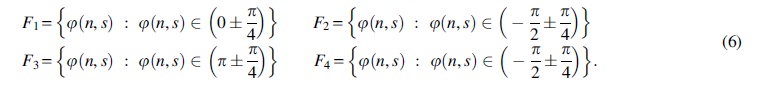
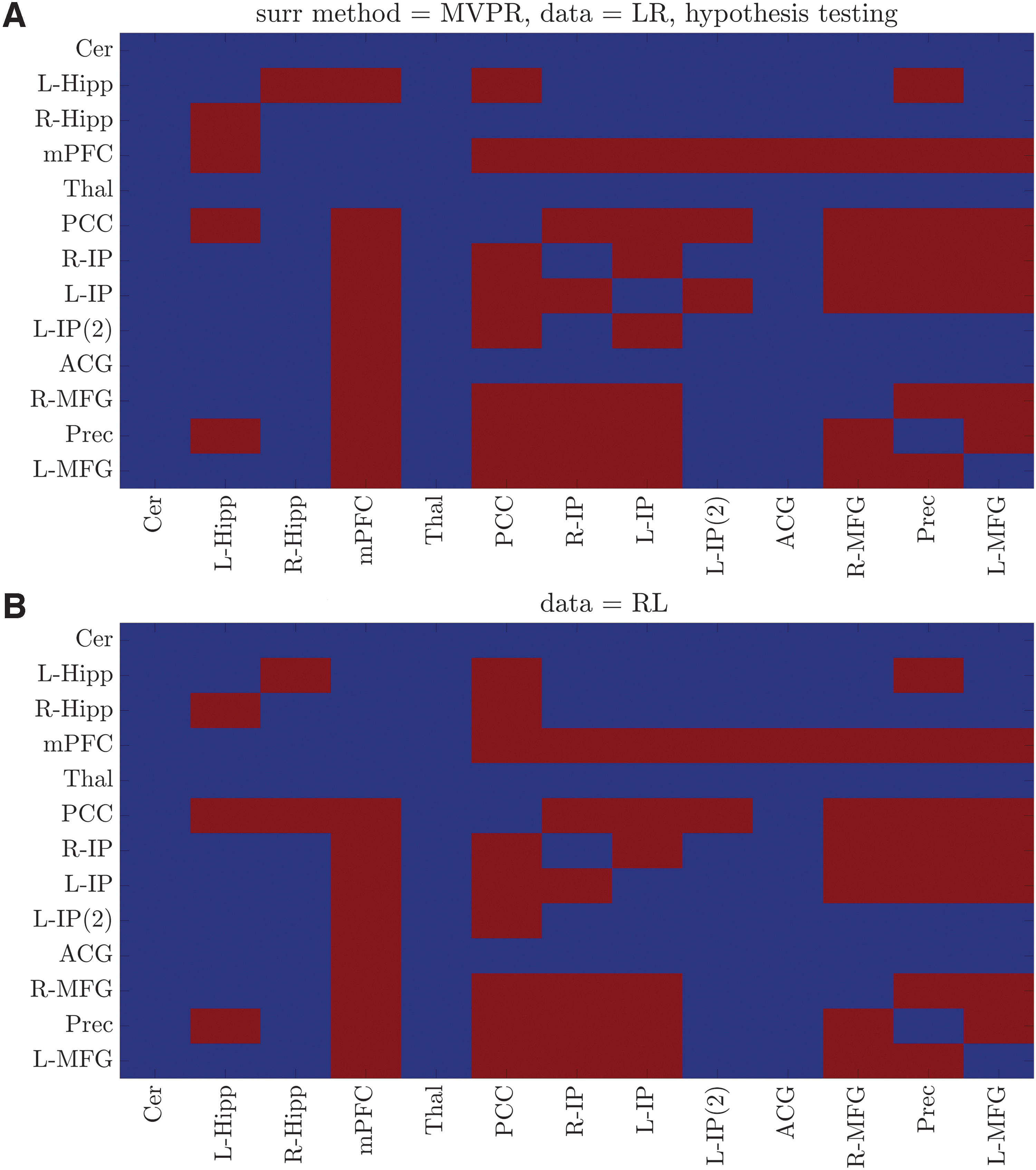
In the case of MVPR (Fig. 3), the identified dynamically connected region pairs were very similar for both datasets (27 of 30 total dynamic connections), suggesting the high reproducibility of the proposed method (90%). Importantly, the identified dynamically connected pairs included regions of the medial prefrontal and posterior cingulate cortices, inferior parietal lobes, and hippocampal formation, which have been previously characterized as the core DMN regions (Buckner et al., 2008). In the case of MVAR method (Fig. 4), the identified dynamic connections were significantly fewer compared with the MVPR approach, contradicting the aforementioned results and those previously presented in other studies (Chang and Glover, 2010; Savva et al., 2019; Zalesky et al., 2014). The large deviations in the results between the two methods were due to their difference in generating surrogate data (Surrogate Data: Properties of Original Data Preserved in Surrogate Time-Series section). As mentioned in the Introduction, methods to create surrogate data aim at preserving key properties of the original data, while lacking the property they are tested for, that is, dFC (Hindriks et al., 2016).

FIG. 3.

Dynamic connections within DMN using the MVPR approach. Dynamically connected region pairs (p < 0.05, Bonferroni corrected) for (A) LR and (B) RL datasets, identified by averaging coherence values across all frequency scales. The identified dynamically connected pairs involve regions of the medial prefrontal and posterior cingulate cortices, inferior parietal lobes and hippocampal formation, which have been characterized as the core DMN regions. ACG, anterior cingulate gyrus; Cer, cerebellum; DMN, default mode network; L-Hipp, left hippocampus; L-IP, left inferior parietal; L-IP(2), left inferior parietal—2; L-MFG, left middle frontal gyrus; MVPR, multivariate phase randomization; Prec, precuneus; R-Hipp, right hippocampus; R-IP, right inferior parietal; RL, right–left encoding; R-MFG, right middle frontal gyrus; Thal, thalamus. Color images are available online.

FIG. 4.

Dynamic connections within DMN using the MVAR approach. Dynamically connected region pairs (p < 0.05, Bonferroni corrected) for (A) LR and (B) RL datasets, identified by averaging coherence values across all frequency scales. Color images are available online.

Two-sessions HCP data: TVRP of dynamically connected region pairs

To assess lead/lag/synchronization patterns (positive/negative correlations), circular histograms were created by assembling TVRP time series from all subjects, for the corresponding region pairs that were found to exhibit dFC (Fig. 3). The results obtained from the MVPR method were used, since this method better preserved properties of the data as shown in Surrogate Data: Properties of Original Data Preserved in Surrogate Time Series section. In the case of a representative example (Fig. 5) for the mPFC–PCC pair, the circular mean (ā, red line) is virtually zero with large (≈0.9) circular spread (r, lack vector), suggesting that apart from being dynamically connected, this region pair was synchronized in activity for both scanning sessions. Results for the remaining region pairs exhibiting dFC are provided in the Supplementary Data (Supplementary Fig. S2). Overall, circular means were found to range between −15° (345°) and 15°, with circular spread >0.6, suggesting that the identified dynamically connected region pairs also exhibited synchronized activity patterns.

FIG. 5.

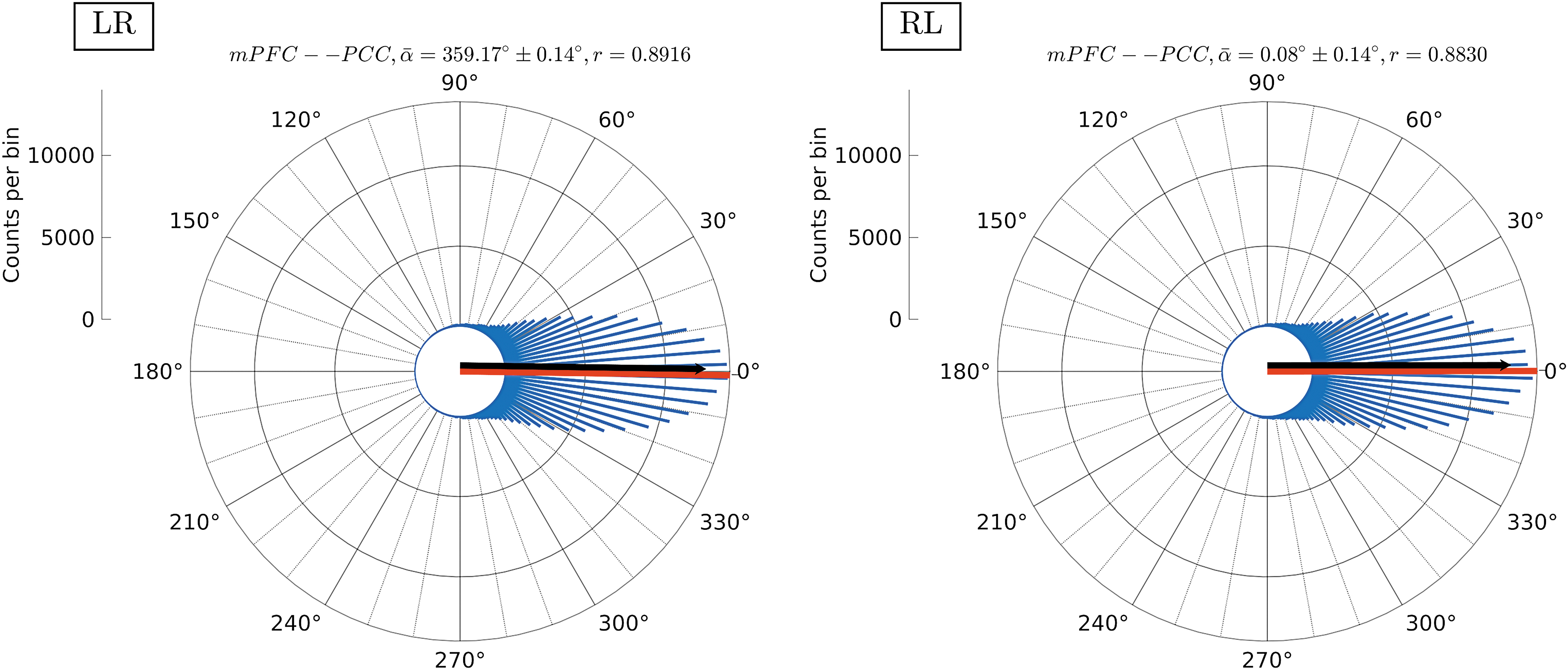
Time-varying relative phase distribution. Circular histograms (blue lines) of mPFC–PCC TVRP values from all subjects for the LR (left panel) and RL (right panel) datasets. TVRP values were estimated by averaging phase values across all frequency scales. The red lines denote the circular mean (ā) and the black vectors denote the circular spread (r) of the data, while the confidence interval of the mean is provided in the title (confidence level of 0.05). The mPFC–PCC pair apart from being dynamically connected (Fig. 3) was synchronized in time for both scanning sessions. Color images are available online.

Two-sessions HCP data: frequency-dependent dFC presence and TVRP

Averaging coherence and relative phase was also applied considering five distinct frequency bands (Time-Varying Functional Connectivity section). The corresponding results using the MVPR surrogates (Figs. 6 and 7; LR and RL datasets, respectively) suggest that the majority of dynamic connections (69 of 75 [LR dataset] and 55 of 58 [RL dataset]) involved the core DMN regions as above, and were identified within the slow-3, slow-4, and slow-5 bands (0.01 Hz < f ≤ 0.198 Hz; 5.1 sec ≤ scale <100 sec). Moreover, the identified dynamic connections varied between the two datasets with test–retest reproducibility of 0%, 60%, 65.63%, 14.71%, and 0% for the slow-2, slow-3, slow-4, slow-5, and slow-6 bands, respectively, suggesting that averaging across all frequency scales yields more robust dFC patterns, whereby test–retest reproducibility was 90%. To extract synchronization patterns, circular histograms were created following the procedure described above, for each frequency band separately. The corresponding results are shown in the Supplementary Data (Supplementary Figs. S3 and S4; LR and RL datasets, respectively), suggesting that the identified dynamic connections once again exhibited synchronized activity patterns, with circular means between −30° (330°) and 30° and circular spreads >0.5.

FIG. 6.

Frequency-dependent dynamic connections within DMN using the MVPR approach. Identified dynamically connected region pairs (LR dataset, p < 0.05, Bonferroni corrected) by averaging coherence values across the specified frequency bands. The majority of dynamic connections were found in the frequency range (0.01, 0.198) Hz (scales between 5.1 and 100 sec) involving the core DMN regions. Color images are available online.

FIG. 7.

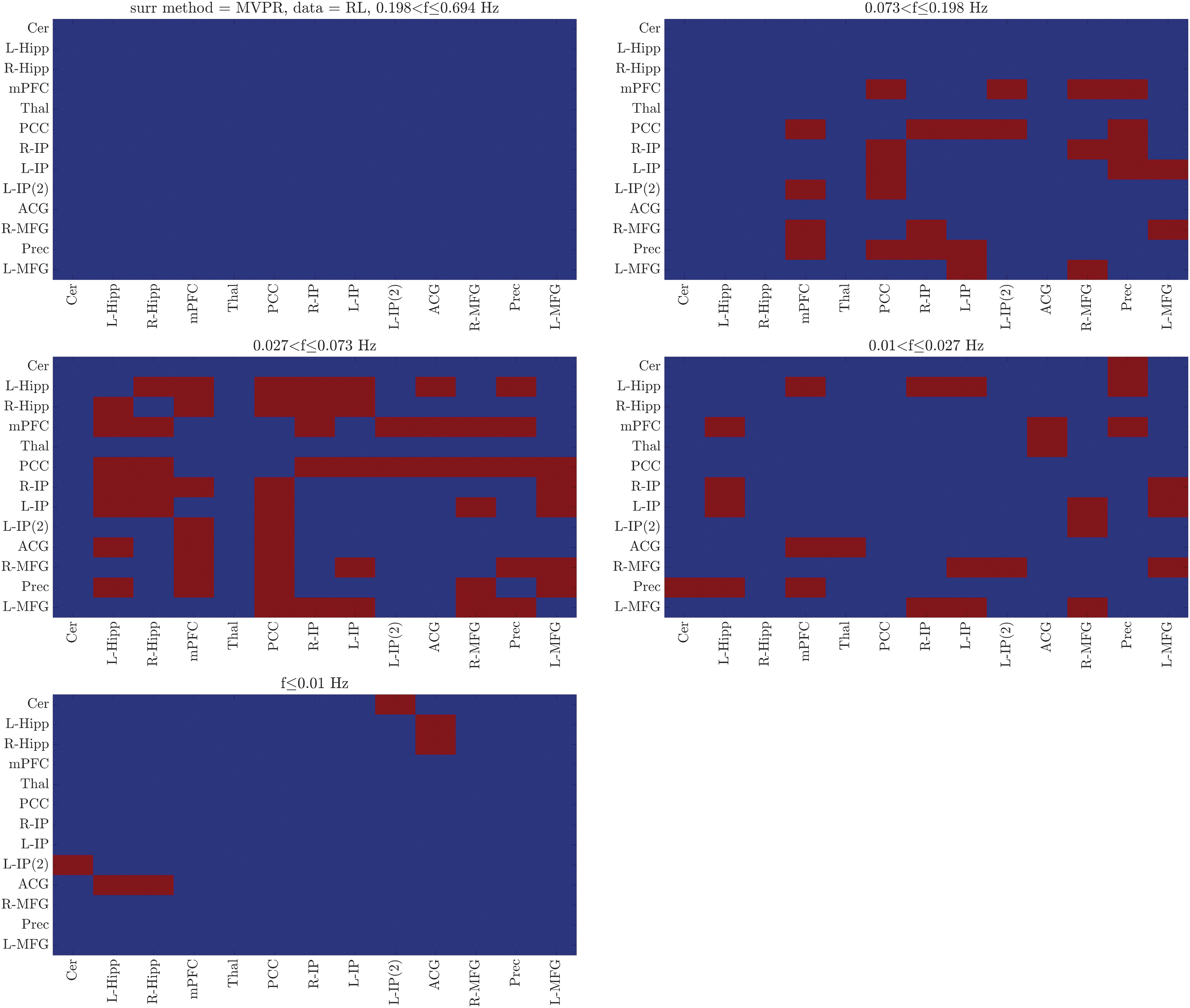
Frequency-dependent dynamic connections within DMN using the MVPR approach. Identified dynamically connected region pairs (RL dataset, p < 0.05, Bonferroni corrected) by averaging coherence values across the specified frequency bands. The majority of dynamic connections were found in the frequency range (0.01, 0.198) Hz (scales between 5.1 and 100 sec) involving the core DMN regions. Color images are available online.

Surrogate data: properties of original data preserved in surrogate time series

A qualitative analysis using the same representative low-motion subject as before (HCP 156536; mean FD = 0.076 mm; LR dataset) is depicted in Section S3 of the Supplementary Data (Supplementary Figs. S5 and S6), with the results providing mostly visual evidence that the MVPR method better preserved properties of the original data as compared with the MVAR approach. To assess in a quantitative manner property preservation, 10 subjects with the lowest mean FD (LR: 0.076–0.094 mm, RL: 0.08–0.1 mm) and 10 with the highest mean FD (LR: 0.1885–0.1987 mm; RL: 0.1869–0.1995 mm) were used, estimating the similarity between the original and surrogate data for both MVPR and MVAR methods. Similarity was assessed in terms of absolute difference for the cross-correlation matrix, the Kullback–Leibler divergence for the amplitude distribution, and the Pearson correlation for the remaining properties, that is, power and cross-power spectral density, autocovariance, and TAC. Lower absolute difference and the Kullback–Leibler divergence values, as well as higher Pearson's correlation values, indicate better agreement between the original and surrogate data.

Similarity metrics were averaged across subjects and region pairs to draw conclusions at the group level, and examine property preserving across all employed ROIs. The corresponding results are shown in Table 2, where the minimum, maximum, and median of each similarity metric are shown. In addition, a Mann–Whitney U-test was performed to evaluate whether there were statistical differences between the obtained values and was favored over paired t-test, since the Kolmogorov–Smirnov tests rejected the null hypothesis that the data were from a standard normal distribution in all cases. In all cases, except amplitude distribution in the LR dataset, the acquired results suggested that properties of the MVPR surrogates were better matched to the original data compared with MVAR surrogates (p < 10⁻¹⁰). Consequently, this suggests that the MVPR method creates surrogate data, which better preserve properties of the original data compared with the MVAR approach.

Table 2.

Similarity Metrics Between Original and Surrogate Data

Data property (similarity metric)	Low FD
	LR							RL
	MVPR			MVAR			p	MVPR			MVAR			p
	Min	Median	Max	Min	Median	Max	p	Min	Median	Max	Min	Median	Max	p
Cross-correlation matrix (absolute difference)	0.0005	0.0005	0.0005	0.0251	0.0341	0.0442	^*	0.0003	0.0003	0.0003	0.0259	0.0334	0.0469	^*
Power spectral density (Pearson's correlation)	0.7703	0.7744	0.7786	0.4671	0.4745	0.4820	^*	0.7658	0.7710	0.7776	0.4563	0.4638	0.4708	^*
Cross-power spectral density (Pearson's correlation)	0.9855	0.9863	0.9870	0.9791	0.9796	0.9801	^*	0.9857	0.9865	0.9873	0.9793	0.9799	0.9805	^*
Amplitude distribution (Kullback–Leibler)	0.0315	0.0330	0.0353	0.0315	0.0330	0.0353	1	0.0290	0.0300	0.0311	0.0303	0.0322	0.0350	^*
Autocovariance (Pearson's correlation)	0.7089	0.7345	0.7613	0.4472	0.4801	0.5395	^*	0.6612	0.6880	0.7062	0.4643	0.4871	0.5131	^*
Time-averaged coherence (Pearson's correlation)	0.4121	0.4738	0.5184	0.0581	0.1153	0.1813	^*	0.4163	0.4694	0.5159	0.0420	0.0894	0.1422	^*

	High FD
	MVPR			MVAR			p	MVPR			MVAR			p
	Min	Median	Max	Min	Median	Max	p	Min	Median	Max	Min	Median	Max	p
Cross-correlation matric (absolute difference)	0.0005	0.0005	0.0005	0.0275	0.0390	0.0552	^*	0.0006	0.0006	0.0006	0.0269	0.0330	0.0447	^*
Power spectral density (Pearson's correlation)	0.7749	0.7804	0.7866	0.4719	0.4798	0.4855	^*	0.7640	0.7694	0.7742	0.4457	0.4532	0.4630	^*
Cross-power spectral density (Pearson's correlation)	0.9816	0.9827	0.9836	0.9712	0.9723	0.9731	^*	0.9830	0.9839	0.9847	0.9741	0.9748	0.9756	^*
Amplitude distribution (Kullback–Leibler)	0.0314	0.0336	0.0392	0.0314	0.0336	0.0392	1	0.0292	0.0300	0.0313	0.0292	0.0304	0.0327	^*
Autocovariance (Pearson's correlation)	0.7202	0.7481	0.7692	0.4384	0.4753	0.5057	^*	0.6840	0.7062	0.7252	0.4580	0.4853	0.5152	^*
Time-averaged coherence (Pearson's correlation)	0.4215	0.4648	0.4979	0.0359	0.0819	0.1367	^*	0.4064	0.4494	0.4973	0.0971	0.1421	0.2106	^*

In almost all cases, properties of MVPR surrogates better matched the original data compared with MVAR surrogates (p < 10^–10; marked with an asterisk), except amplitude distribution in the LR dataset (p = 1).

FD, framewise displacement; LR, left–right encoding; MVAR, multivariate autoregressive randomization; MVPR, multivariate phase randomization; RL, right–left encoding.

Discussion

Summary

In this study, we employed the wavelet-based method proposed in Chang and Glover (2010), and modified it to measure temporal variability using the coherence magnitude and synchronization patterns using the relative phase. To this end, we examined two approaches: (1) coherence magnitude and relative phase were averaged across all frequency scales (Two-Sessions HCP Data: Statistically Significant Fluctuations in TVFC (dFC Presence) section and Two-Sessions HCP Data: TVRP of Dynamically Connected Region Pairs section), and (2) coherence magnitude and relative phase were averaged across distinct frequency bands (Two-Sessions HCP Data: Frequency-Dependent dFC Presence and TVRP section). To define the null hypothesis of dFC absence, the MVPR and MVAR surrogate data generation methods were used.

The main finding of this study is the identification of dynamic connections within the DMN, which were very similar between the two datasets (test–retest reproducibility 90% when averaging coherence magnitude across all frequency scales). By repeating the analysis within distinct frequency bands, the majority of dynamic connections were identified in the frequency range (0.01, 0.198) Hz, though with lower test–retest reproducibility (<66%), suggesting that averaging across all frequency scales yields more robust dFC estimates. The identified dynamic connections were in agreement with previous studies (Chang and Glover, 2010; Savva et al., 2019; Zalesky et al., 2014) and exhibited synchronization patterns (relative phase was found to be between [−15°, 15°]). Further evaluation suggested that MVPR method better preserved properties of the original data (p < 10⁻¹⁰), including TAC, which is shown to be preserved for the first time to our knowledge.

The main difference of the proposed approach compared with that reported in Chang and Glover (2010) is that we incorporated information from all frequency scales, by averaging wavelet coherence magnitude and relative phase across scales, whereas in Chang and Glover (2010) different frequency scales were treated independently. Using this approach, they presented evidence of (frequency) scale-dependent, nonstationary variation for each subject separately, whereas in this study we applied the proposed method to obtain conclusions at the group level, yielding more reproducible results compared with narrow bands. To this end, we employed a large dataset comprising of 200 subjects with 2 scanning sessions each, formulating a test–retest approach, while in Chang and Glover (2010) 12 subjects were used. Finally, Chang and Glover (2010) used the bivariate AR approach to create surrogate data, while in this study the multivariate approach was used following recent evidence that the bivariate approach may introduce a large number of false positives (Liegeois et al., 2017).

Wavelet analysis versus sliding window method

Wavelet analysis provides a significant advantage over the sliding window method, by circumventing the need to select a fixed window size (which may have significant effect on the final results), since it becomes an internal parameter of the method, that is, scale in Eq. (1) (Torrence and Compo, 1998). In our previous study, a wide range of window sizes (20–150 sec) along with 10 FC metrics were employed to assess the presence of dFC within DMN, suggesting that the identified dynamic connections were both window length and FC metric specific. Specifically, for each combination of window size and FC metric a generally different number of dynamically connected region pairs were identified (hypothesis testing was also based on MVPR surrogates) ranging from none to 37 (Savva et al., 2019). These results demonstrate the potentially significant effects of the window length and despite the growing literature, there is, to date, no consensus on the optimal window size value for estimating fMRI-based dFC (see Introduction section; Lurie et al., 2020; Preti et al., 2017).

The sliding window also requires the selection of FC metric, while window functions other than the rectangular have been associated with the suppression of motion-related noise that likely remains in the data even after preprocessing (see Introduction section; Allen et al., 2014; Hutchison et al., 2013a; Lindquist et al., 2014; Preti et al., 2017). Nevertheless, in a recent study it was suggested that such window functions may also suppress true time-varying fluctuations in FC (Savva et al., 2020).

Overall, these results suggest that in the absence of ground truth (Shakil et al., 2016), the identified dynamic connections are dependent on the original choice of sliding window parameters, and alternative methods may be advantageous. In this context, the wavelet approach requires only the selection of the wavelet basis function. This choice may also pose some challenges, since it is associated with the ability to extract time–frequency information from the original signal according to the shape of the basis function.

In this study, the Morlet wavelet was employed, which has been also used in previous fMRI studies (Chang and Glover, 2010; Wang et al., 2017; Yaesoubi et al., 2015, 2017). However, this does not necessarily suggest that the Morlet wavelet is the optimal basis function for estimating TVFC in rs-fMRI, and future work could explore the relationship between TVFC patterns and dynamic connections with other wavelet basis functions, such as Paul wavelets and derivatives of Gaussian (Torrence and Compo, 1998).

On hypothesis testing formulation

In Liegeois et al. (2017), a thorough investigation was performed to clarify issues regarding stationarity and statistical testing, with the authors providing some definitions aiming to resolve potential confusion in the literature. Specifically, we adopted the term “time-varying functional connectivity” to indicate fluctuations of FC as a function of time, while we defined “dynamic functional connectivity” to signify statistically significant fluctuations in FC. Statistical significance was assessed comparing variance of TVFC from original data with the corresponding values from surrogate data using the MVPR method, which generates data that are stationary, linear, and Gaussian (Liegeois et al., 2017). Moreover, it must be taken into consideration that physiological factors (arterial CO₂, heart rate, and heart-rate variability) affect TVFC estimates, apart from neuronal activity as measured by fMRI (Nikolaou et al., 2016). As a result, the rejection of null hypothesis is due to any combination of (or all) nonstationarity, nonlinearity, non-Gaussianity (Liegeois et al., 2017), as well as due to physiological factors, such as arterial CO₂, heart rate, and heart-rate variability (Nikolaou et al., 2016).

dFC patterns

The results of hypothesis testing (Two-Sessions HCP Data: Statistically Significant Fluctuations in TVFC (dFC Presence) section and Two-Sessions HCP Data: Frequency-Dependent dFC Presence and TVRP section) suggested that regions of the DMN (Buckner et al., 2008), involving medial prefrontal and posterior cingulate cortices, inferior parietal lobes and hippocampal formation, exhibited dFC (Figs. 3, 6, and 7). These results are in agreement with previous studies using either wavelet (Chang and Glover, 2010) or sliding window approaches (Savva et al., 2019; Zalesky et al., 2014). Specifically, Chang and Glover (2010) suggested that dynamic associations were observed between the PCC positively correlated regions (mPFC, L/R-IP) using a wavelet method similar to this study. On the contrary, and despite its potential drawbacks as mentioned above, Zalesky et al. (2014) employed the sliding window method with Pearson's correlation and an exponentially weighted window shape of 60 sec length, to identify 19 parietal and frontal regions exhibiting dFC, while in our previous study the use of sliding window approach with nonlinear metrics (mutual information and variation of information) in conjunction with a rectangular window size of 120 sec suggested that region pairs involving mPFC, PCC, L/R-IP, Prec, and L/R-MFG exhibited dFC (Savva et al., 2019).

Finally, the analysis of circular histograms (Two-Sessions HCP Data: TVRP of Dynamically Connected Region Pairs section and Two-Sessions HCP Data: Frequency-Dependent dFC Presence and TVRP section) suggested that the identified dynamically connected region pairs were also synchronized in activity (circular means between −15° and 15°). These results are in agreement with a previous study (Chang and Glover, 2010), where pairs between PCC and mPFC, L/R-IP were found to exhibit relative phase values in the interval (−π/4, π/4).

The DMN dynamic functional organization

To further examine the role of each region that exhibited dFC, the number of dynamic connections per ROI was calculated (Fig. 8), for the first approach, with the mPFC, PCC, L/R-IP, and L/R-MFG being found to be involved in the majority of dynamic connections, suggesting their pivotal role during the resting state and the functional connection between the frontal and posterior areas of the brain. In fact, previous studies in rs-fMRI have identified PCC, mPFC, and L/R angular gyrus as functional hubs (Buckner et al., 2008; de Pasquale et al., 2018), using weighted and nonweighted global brain connectivity methods (Cole et al., 2010), or with correlation approaches at various significance levels (de Pasquale et al., 2013). Apart from rs-fMRI, magnetoencephalography has been employed to examine dependencies between six resting-state networks (dorsal and ventral attention, DMN, visual, somatomotor, and language), suggesting that on the network level, the DMN exhibited particularly high interaction (p < 0.005) to the other networks within the β-band (14–25 Hz) (de Pasquale et al., 2012). Moreover, the authors have identified the PCC as the region with pronounced interaction level (p < 0.001) with other regions of the brain, not necessarily belonging to the DMN, while L/R angular gyrus and ventral/right prefrontal cortices exhibited interactions at a slightly lower level (p < 0.05) to other areas of the brain (de Pasquale et al., 2012). In this study, the aforementioned region pairs were found to be involved in the majority of dynamic connections, also suggesting their central role within the DMN.

FIG. 8.

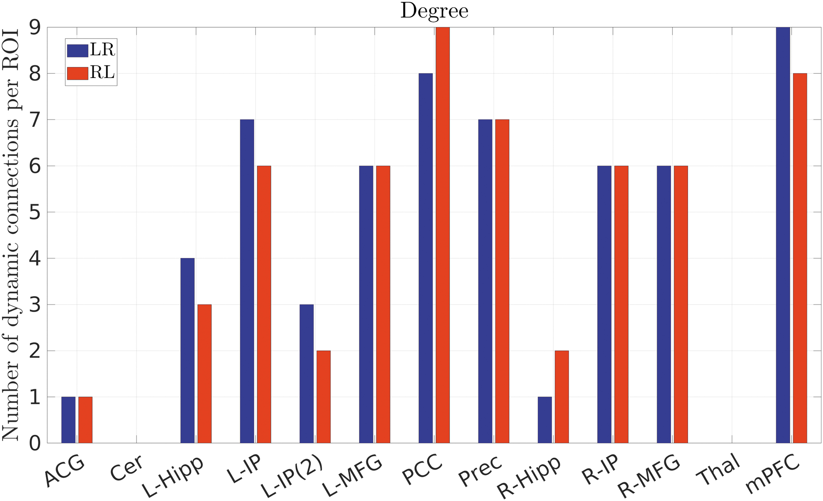
Number of dynamic connections for each region. The mPFC, PCC, L/R-IP, and L/R-MFG were found to be involved in the majority of dynamic connections. Color images are available online.

Another study examined whether dFC can identify links to daydreaming, finding that dynamic connections between the PCC and somatomotor/primary visual networks were positively correlated with an index quantifying daydreaming, that is, daydreaming frequency scale (Kucyi and Davis, 2014). These results led the authors to suggest that the PCC is likely a major hub (Hagmann et al., 2008), which serves as a dynamic arbitrator between other regions of the brain, either part of DMN or other networks (Kucyi and Davis, 2014).

Conclusions

The proposed wavelet-based approach can reliably assess dFC with fewer choices in terms of hyperparameters, compared with the sliding window method. In this context, dynamic connections were identified using 400 high-quality, low-motion rs-fMRI data from 200 subjects, forming a test–retest approach, suggesting the high reproducibility (90%) of the method when averaging coherence magnitude and phase across all frequencies. Dynamic connections were also identified by averaging across frequency bands, the majority of which were found from 0.01 to 0.198 Hz, though with lower test–retest reproducibility (<66%), suggesting that averaging across all frequency scales yields more robust dFC patterns. In addition, the identified dynamic connections were synchronized in activity (−15° ≤ phase ≤15°), while further analysis suggested that the MVPR method better preserved (p < 10⁻¹⁰) the properties of the original data, including TAC.

Footnotes

Acknowledgments

We thank Christos Efrem, School of Electrical and Computer Engineering, National Technical University of Athens for useful discussions regarding wavelet methodology. Data were provided by the HCP, WU-Minn Consortium (Principal Investigators: David Van Essen and Kamil Ugurbil; 1U54MH091657) funded by the 16 NIH Institutes and Centers that support the NIH Blueprint for Neuroscience Research; and by the McDonnell Center for Systems Neuroscience at Washington University.

Authors' Contributions

A.D.S. contributed to conceptualization, methodology, software, formal analysis, data curation, writing—original draft; G.K.M. and G.D.M. also contributed to conceptualization, methodology, writing—review and editing, supervision.

Author Disclosure Statement

No competing financial interests exist.

Funding Information

No funding was received for this article.

Supplementary Material

Supplementary Data

Supplementary Figure S1

Supplementary Figure S2

Supplementary Figure S3

Supplementary Figure S4

Supplementary Figure S5

Supplementary Figure S6

References

Allen

, Damaraju

, Plis

, et al. 2014. Tracking whole-brain connectivity dynamics in the resting state. Cereb Cortex, 24:663–676.

Andrews-Hanna

, Reidler

, Sepulcre

, et al. 2010. Functional-anatomic fractionation of the brain's default network. Neuron, 65:550–562.

Berens

. 2009. CircStat: AMATLABToolbox for circular statistics. J Stat Softw, 31:21.

Buckner

, Andrews-Hanna

, Schacter

. 2008. The brain's default network: anatomy, function, and relevance to disease. Ann N Y Acad Sci, 1124:1–38.

Chang

, Glover

. 2010. Time-frequency dynamics of resting-state brain connectivity measured with fMRI. Neuroimage, 50:81–98.

Cole

, Pathak

, Schneider

. 2010. Identifying the brain's most globally connected regions. Neuroimage, 49:3132–3148.

Damoiseaux

, Rombouts

SARB

, Barkhof

, et al. 2006. Consistent resting-state networks across healthy subjects. Proc Natl Acad Sci, 103:13848–13853.

de Pasquale

, Corbetta

, Betti

, et al. 2018. Cortical cores in network dynamics. Neuroimage, 180:370–382.

de Pasquale

, Della Penna

, Snyder

, et al. 2012. A cortical core for dynamic integration of functional networks in the resting human brain. Neuron, 74:753–764.

10.

de Pasquale

, Sabatini

, Della Penna

, et al. 2013. The connectivity of functional cores reveals different degrees of segregation and integration in the brain at rest. Neuroimage, 69:51–61.

11.

Di Martino

, Ghaffari

, Curchack

, et al. 2008. Decomposing intra-subject variability in children with attention-deficit/hyperactivity disorder. Biol Psychiatry, 64:607–614.

12.

Glasser

, Sotiropoulos

, Wilson

, et al. 2013. The minimal preprocessing pipelines for the Human Connectome Project. Neuroimage, 80:105–124.

13.

Grinsted

, Moore

, Jevrejeva

. 2004. Application of the cross wavelet transform and wavelet coherence to geophysical times series. Nonlinear Processes Geophys, 11:561–566.

14.

Hagmann

, Cammoun

, Gigandet

, et al. 2008. Mapping the structural core of human cerebral cortex. PLoS Biol, 6:e159.

15.

Hindriks

, Adhikari

, Murayama

, et al. 2016. Can sliding-window correlations reveal dynamic functional connectivity in resting-state fMRI?. Neuroimage, 127:242–256.

16.

Hramov

, Koronovskii

, Makarov

, et al. 2014. Wavelets in Neuroscience. New York: Springer Berlin. Heidelberg.

17.

Hutchison

, Womelsdorf

, Allen

, et al. 2013a. Dynamic functional connectivity: promise, issues, and interpretations. Neuroimage, 80:360–378.

18.

Hutchison

, Womelsdorf

, Gati

, et al. 2013b. Resting-state networks show dynamic functional connectivity in awake humans and anesthetized macaques. Hum Brain Mapp, 34:2154–2177.

19.

Jammalamadaka

, Sengupta

. 2001. Topics in Circular Statistics. Singapore City, Singapore: World Scientific Publishing Co. Pte. Ltd.

20.

Kucyi

, Davis

. 2014. Dynamic functional connectivity of the default mode network tracks daydreaming. Neuroimage, 100:471–480.

21.

Liegeois

, Laumann

, Snyder

, et al. 2017. Interpreting temporal fluctuations in resting-state functional connectivity MRI. Neuroimage, 163:437–455.

22.

Lindquist

, Xu

, Nebel

, Caffo

. 2014. Evaluating dynamic bivariate correlations in resting-state fMRI: a comparison study and a new approach. Neuroimage, 101:531–546.

23.

Liu

, Duyn

. 2013. Time-varying functional network information extracted from brief instances of spontaneous brain activity. Proc Natl Acad Sci U S A, 110:4392–4397.

24.

Lurie

, Kessler

, Bassett

, et al. 2020. Questions and controversies in the study of time-varying functional connectivity in resting fMRI. Netw Neurosci, 4:30–69.

25.

Majeed

, Magnuson

, Hasenkamp

, et al. 2011. Spatiotemporal dynamics of low frequency BOLD fluctuations in rats and humans. Neuroimage, 54:1140–1150.

26.

Nikolaou

, Orphanidou

, Papakyriakou

, et al. 2016. Spontaneous physiological variability modulates dynamic functional connectivity in resting-state functional magnetic resonance imaging. Philos Trans A Math Phys Eng Sci, 374:20150183.

27.

Power

, Barnes

, Snyder

, et al. 2012. Spurious but systematic correlations in functional connectivity MRI networks arise from subject motion. Neuroimage, 59:2142–2154.

28.

Preti

, Bolton

, Van De Ville

. 2017. The dynamic functional connectome: state-of-the-art and perspectives. Neuroimage, 160:41–54.

29.

Raichle

, MacLeod

, Snyder

, et al. 2001. A default mode of brain function. Proc Natl Acad Sci U S A, 98:676–682.

30.

Savva

, Kassinopoulos

, Smyrnis

, et al. 2020. Effects of motion related outliers in dynamic functional connectivity using the sliding window method. J Neurosci Methods, 330:108519.

31.

Savva

, Mitsis

, Matsopoulos

. 2019. Assessment of dynamic functional connectivity in resting-state fMRI using the sliding window technique. Brain Behav, 9:e01255.

32.

Shakil

, Lee

, Keilholz

. 2016. Evaluation of sliding window correlation performance for characterizing dynamic functional connectivity and brain states. Neuroimage, 133:111–128.

33.

Shirer

, Ryali

, Rykhlevskaia

, et al. 2012. Decoding subject-driven cognitive states with whole-brain connectivity patterns. Cereb Cortex, 22:158–165.

34.

Smith

, Beckmann

, Andersson

, et al. 2013. Resting-state fMRI in the human connectome project. Neuroimage, 80:144–168.

35.

Smith

, Miller

, Moeller

, et al. 2012. Temporally-independent functional modes of spontaneous brain activity. Proc Natl Acad Sci U S A, 109:3131–3136.

36.

Torrence

, Compo

. 1998. A practical guide to wavelet analysis. Bull Am Meteorol Soc, 79:61–78.

37.

Torrence

, Webster

. 1999. Interdecadal changes in the ENSO-monsoon system. J Clim, 12:2679–2690.

38.

Van Essen

, Smith

, Barch

, Behrens

, et al. 2013. The WU-Minn human connectome project: an overview. Neuroimage, 80:62–79.

39.

Varoquaux

, Craddock

. 2013. Learning and comparing functional connectomes across subjects. Neuroimage, 80:405–415.

40.

Wang

, Yang

, Chen

. 2017. Abnormal dynamics of cortical resting state functional connectivity in chronic headache patients. Magn Reson Imaging, 36:56–67.

41.

Yaesoubi

, Allen

, Miller

, Calhoun

. 2015. Dynamic coherence analysis of resting fMRI data to jointly capture state-based phase, frequency, and time-domain information. Neuroimage, 120:133–142.

42.

Yaesoubi

, Miller

, Bustillo

, et al. 2017. A joint time-frequency analysis of resting-state functional connectivity reveals novel patterns of connectivity shared between or unique to schizophrenia patients and healthy controls. NeuroImage Clin, 15:761–768.

43.

Zalesky

, Fornito

, Cocchi

, et al. 2014. Time-resolved resting-state brain networks. Proc Natl Acad Sci U S A, 111:10341–10346.

44.

Zittrell

. 2019. CircHist: circular histogram in MATLAB. Zenodo. DOI: 10.5281/zenodo.3445084.

45.

Zuo

, Di Martino

, Kelly

, et al. 2010. The oscillating brain: complex and reliable. Neuroimage, 49:1432–1445.

Supplementary Material

Please find the following supplemental material available below.

For Open Access articles published under a Creative Commons License, all supplemental material carries the same license as the article it is associated with.

For non-Open Access articles published, all supplemental material carries a non-exclusive license, and permission requests for re-use of supplemental material or any part of supplemental material shall be sent directly to the copyright owner as specified in the copyright notice associated with the article.

0.00 MB

1.17 MB

0.66 MB

10.33 MB

15.04 MB

11.60 MB

0.28 MB