Threshold Selection for Brain Connectomes

Abstract

Introduction:

Structural and functional brain connectomes represent macroscale data collected through techniques such as magnetic resonance imaging (MRI). Connectomes may contain noise that contributes to false-positive edges, thereby obscuring structure-function relationships and data interpretation. Thresholding procedures can be applied to reduce network density by removing low-signal edges, but there is limited consensus on appropriate selection of thresholds. This article compares existing thresholding methods and introduces a novel alternative “objective function” thresholding method.

Methods:

The performance of thresholding approaches, based on percolation and objective functions, is assessed by (1) computing the normalized mutual information (NMI) of community structure between a known network and a simulated, perturbed networks to which various forms of thresholding have been applied, and by (2) comparing the density and the clustering coefficient (CC) between the baseline and thresholded networks. An application to empirical data is provided.

Results:

Our proposed objective function-based threshold exhibits the best performance in terms of resulting in high similarity between the underlying networks and their perturbed, thresholded counterparts, as quantified by NMI and CC analysis on the simulated functional networks.

Discussion:

Existing network thresholding methods yield widely different results when graph metrics are subsequently computed. Thresholding based on the objective function maintains a set of edges such that the resulting network shares the community structure and clustering features present in the original network. This outcome provides a proof of principle that objective function thresholding could offer a useful approach to reducing the network density of functional connectivity data.

Impact statement

Network thresholding refers to removing edges between node pairs in a functional network that have weak edge-weights potentially arising from unwanted variability or noise. Since edge-weight cutoffs used to generate a binary network can be sensitive to the thresholding method, we introduce a novel thresholding algorithm. We find that when applied to networks derived via perturbations, namely through simulated functional connectivity of a known network, our approach yields a binary network that is more similar to the known network compared with using existing thresholding approaches. Our algorithm is a competitive candidate for thresholding brain connectomes.

Introduction

Network representations of biological data produce graphs that are weighted but complete, consist of low-signal edges (van den Heuvel et al., 2017), or are sparse but contaminated with false positives (Drakesmith et al., 2015; Pu et al., 2015). A functional connectome (FC) generated from functional magnetic resonance imaging (fMRI) data consists of edges that are defined by correlations between nodal time series of blood oxygenation level dependent (BOLD) signals.

Weighted networks can include weakly correlated regions that may represent noise. In the structural connectome (SC) built using anisotropy-based diffusion streamlines, false positives are less prevalent but still possible (Sotiropoulos and Zalesky, 2019).

Network thresholding is crucial to elucidate differences between study groups in a reproducible manner. A threshold can be applied to create less dense binarized or weighted graphs from fully connected graphs (Bassett et al., 2008), or to remove false positive edges (Drakesmith et al., 2015). Nevertheless, aggressive thresholding approaches produce very sparse graphs whereas overly cautious approaches produce graphs containing noise-driven connections, impugning the accuracy of subsequently calculated graph metrics.

For real-world applications of graph theory such as in psychiatry, these issues confound the interpretation of differences in graph measures between clinical groups. Despite the importance of thresholding, a few comparisons among existing methods have been made in the literature to evaluate thresholding techniques.

Comparing thresholding techniques can be challenging. Existing thresholding methods sometimes apply to distinct settings or give different network metrics. Some early thresholding methods, such as the small-worldness (σ) range (Bassett et al., 2008), provide a range of thresholds, but not a specific threshold with discernible optimality properties.

The σ-range approach also requires that the networks themselves have small-world properties, thereby limiting its application. Statistical thresholding (Chen et al., 2008; Ferrarini et al., 2009) requires that edge weights have associated metadata, such as p-values for correlations, that are not attributed to all biological networks, and ultimately also require the researcher to select a cutoff value for statistical significance. For example, SC networks of diffusion streams do not have an associated p-value.

More recent methods rely on downstream classifier accuracy to detect the best network threshold (Drakesmith et al., 2015; Zanin et al., 2012), for example, the “multi-threshold permutation correction” method (Drakesmith et al., 2015) involves determining an optimal threshold by clustering thresholded networks into groups and evaluating which threshold yields the most accurate classification. While these methods are applicable to networks with a variety of structures, not just small world-ness, they cannot be performed on a single graph or on a collection of graphs from a single or multiple unknown groups.

Employing the percolation threshold, defined as the highest threshold value for which a network's giant connected component (GCC) includes all nodes, circumvents these difficulties. Although it is a straightforward and reasonable selection method, it does not apply to networks that are not fully connected without any thresholding, that is, the GCC of the network is not the full set of nodes (Bordier et al., 2017). For example, in resting-state fMRI, many nodes might not show significant activation, whereas in task-fMRI some nodes might not participate in processing a task.

It is difficult to define a universal performance measure for outcomes of thresholding. The normalized mutual information (NMI) is useful to compare different thresholding methods. The NMI provides a comparison between the community structures identified within any pair of networks defined on the same set of nodes, each featuring at least two communities (Alexander-Bloch et al., 2012).

If both networks being compared have been subject to thresholding, then this comparison is problematic (e.g., making both networks very sparse might yield a high NMI but be based on communities that bear little resemblance to those present in the true positive edges in the original graphs). Such a comparison is also not possible if the graphs do not exhibit community structure.

To overcome these challenges, and to offer a more universally applicable, easy-to-implement option for thresholding, we introduce a method based on calculating an objective function that uses a simple optimization approach to compute an edge weight threshold for any given network, based on any measure of graph property related to the edges that it includes, or graph metric, such as characteristic path length (λ).

The objective function is based on computing a graph metric over a range of reasonable thresholds, chosen to yield thresholded graphs that are connected but have graph density <1. The selected threshold yields an extremum of an objective function that we define, representing maximal deviation of the graph metric from its value at the extremes of the threshold range, which are where the graph's density is too high, or its GCC is too small.

To demonstrate the performance of this method, we start from a computationally generated, ground truth network designed to exhibit a certain community structure (Lancichinetti et al., 2008) and we introduce fMRI-like noise (Welvaert et al., 2011) to perturb the starting networks into fully connected networks inspired by functional networks.

We compare the performance of the objective function threshold (OFT) with other thresholding methods when applied to these perturbed networks, in terms of their success in restoring the community structure, density, and clustering properties of the ground truth network. We then show an application of the OFT to real data from the UK Biobank (Smith et al., 2020).

Methods

Material Transfer Agreement for access to the UBiobank data was made under University of Pittsburgh IRB approved study number 19020372.

Lancichinetti-Fortunato-Radicchi simulations

To evaluate the effectiveness of thresholding techniques, we generated a sample of networks using a published approach (Bordier et al., 2017). First, a benchmark Lancichinetti-Fortunato-Radicchi (LFR) (Lancichinetti et al., 2008) network is produced, where the true community structure is known. The LFR networks were generated using 363 nodes because the Human Connectome Project (HCP) multimodal atlas has 360 nodes plus brainstem and left and right subcortex (Glasser et al., 2016).

The LFR networks require community mixing parameters to be specified, which were selected based on the guidance of previous use of the LFR benchmark algorithm for network neuroscience applications (Bordier et al., 2017). Next, fMRI-like noise (Welvaert et al., 2011) was introduced to each LFR network to produce a corresponding fully dense (density = 1) simulated FC using parameters based on previous work (Bordier et al., 2017), namely: 363 nodes with an average degree of 24, maximum target degree of 107, community size minimum of 12 and maximum of 32 nodes, with both the community mixing and weight mixing coefficients set to 0.2.

For the simulated FC parameters, a signal-to-noise ratio of 35 was used and 100 replicates were examined to simulate the acquisition of 100 fMRI connectomes. Each replicate was generated from the same LFR network, so all simulated FC replicates share the same ground truth modular structure.

The effectiveness with which thresholding of the simulated FC replicates for noise removal recovers the properties of the benchmark LFR network could then be evaluated, across a variety of thresholding approaches. To do this, the NMI between the known community assignments of the original LFR network and the community structure detected in the noisy LFR networks after thresholding were compared among thresholding techniques (Bordier et al., 2017).

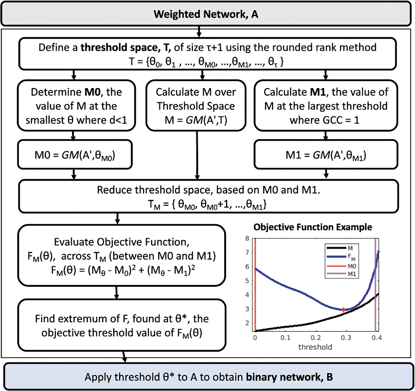
Other measures, such as nodal density and clustering coefficients (CCs) of the binary networks, were also compared with the original LFR network for additional network-specific performance measures. Figure 1 shows an overview of the experimental design.

FIG. 1.

The experimental design for the study. (A) Data generation consists of LFR synthesis, followed by 100 replicates of functional MRI-like noise addition. (B) Threshold application is proceeded by either absolute value of the weighted FC simulated networks to preserve strong negative as positives, or by “zeroing out” the negative values under the assumption that negative edges overwhelming represents node pairs in the LFR network that are not directly connected. These considerations only apply to the percolation threshold, objective function, and maximum spanning tree. A fully weighted network “no threshold” network is included as a “negative control.” (C) Performance of the thresholding methods are compared using NMI, density, and CC accuracy as compared with the original LFR network. CC, clustering coefficient; FC, functional connectome; LFR, Lancichinetti-Fortunato-Radicchi; MRI, magnetic resonance imaging; NMI, normalized mutual information.

Threshold space

Network thresholding provides a cutoff to convert a weighted network into a binary network consisting of presumed true positive edges, such that the original edges with weights at a given threshold, ϴ, are set to zero, while all other original edge weights are set to the value one. We use the term “threshold space” to refer to the set of threshold values tested when evaluating a range of thresholding choices, for example, a natural approach might be to consider a set of possible thresholds between two values ϴ₀ and ϴ₁, separated by a fixed step size ɛ, in which case our threshold space would be the vector of values (ϴ_0, ϴ₀ + ɛ, ϴ₀ + 2ɛ, …, ϴ₁ − ɛ, ϴ₁), assuming that (ϴ₁ − ϴ₀)/ɛ is a positive integer.

A threshold space is not unique to a specific thresholding method, but it is a critical ingredient in a given method's implementation. A “complete” threshold space would include every unique edge weight in a network, to the highest numerical precision possible. Since this choice is impractical in terms of computation time for large networks or large numbers of networks, we define a “rounded rank” threshold space. This is the set of unique edge weights, ranked lowest to highest, after rounding all weights to the nearest thousandth place.

Ranked versus combinatorial thresholding

A distinction can be made between a “ranked” threshold space and a “combinatorial” thresholding method. Unlike a ranked approach, a combinatorial method can remove edges that have larger weights than some of the edges it preserves, for example, statistical thresholding and maximum spanning tree (MST). Most thresholding methods operate on a ranked basis.

Negative edge weights

In networks with some edges having negative weights, a positive threshold will force the zeroing out of all negative weights whereas in networks where edge weights correspond to a count or level of a physical object, such as number of diffusion streams in SC, negative edge weights could result from noise or error and hence their removal is appropriate. In other cases, negative edge weights can pose a challenge for network thresholding, for example, in a network with edge weights based on correlations; large negative values actually represent stronger relationships than near-zero negative values.

In this situation, applying the absolute value function to all network edges before defining a threshold space could be an appropriate step to ensure that thresholding will preserve strongly negative edges and not the weakly negative edges. We apply both approaches in our analysis.

Graph metric calculations

Graph metrics, including density, CC, λ, modular structure, and the size of the GCC, were calculated using the Brain Connectivity Toolbox in MATLAB (Rubinov and Sporns, 2010). For modular structure, the community detection algorithm implemented in the Brain Connectivity Toolbox relies on the Newman method (Newman, 2006), which is a spectral partitioning method that expresses this maximization problem in terms of a matrix eigenvector. The communities are determined by searching for the community structure that maximizes the modularity coefficient (Q).

In networks that have GCC <100% of the nodes, that is, where disjointed sub-graphs appear, the calculation of λ treats the disconnected components as separate networks and averages their results, ignoring pairs of nodes that are not in the same component.

Percolation threshold

When a ranked threshold space is used, a larger threshold results in the removal of more edges. The percolation threshold is defined as the largest ranked threshold at which the network's GCC contains all nodes in the network (Bordier et al., 2017), such that the network is connected. This threshold aims at finding the optimal balance between information gained by noise removal and information lost by excessive pruning of edges, assuming that all nodes belong to the same network.

We will use the notation GCC = 1 to indicate that 100% of the nodes in a network are in its GCC and the notation GCC = x for values between 0 and 1 to indicate the fraction of nodes in the GCC when the network is no longer connected. The percolation method and the MST both provide binary networks with GCC = 1; the former is the strictest possible “ranked” threshold to achieve this, and the latter the strictest possible “combinatorial” threshold.

Objective function threshold

We developed the OFT method under the assumption that the optimal threshold for any weighted network lies between the smallest threshold for which the network density is not 1, and the largest threshold for which the GCC includes the experimentally determined percentage of nodes, here 100%. The objective threshold is determined by first employing a threshold sweep where a range of possible thresholds are evaluated. A MATLAB implementation is provided online via GitHub.

For a given graph measure, M, or any other scalar graph summary metric, the optimal threshold should maximize the difference of this metric from the value of the same metric at both end-points of the threshold space, termed M ₀ and M ₁. The objective function can be maximized/minimized across this range to find the optimal threshold for a given graph metric in any weighted network (Fig. 2).

FIG. 2.

NMI was calculated between the LFR ground-truth community structure and the N = 100 FC_sim networks after thresholding, using the objective function method with GCC = 1 and rounded rank (to the nearest thousandth) threshold space, and one of six choice of graph measure (M). Absolute value of weighted networks was used, and removing negatives was not assessed for this comparison. Density, average nodal degree, λ, transitivity, average CC, and efficiency were compared to identify the best choice of M in the objective function for this application. The highest NMI was achieved with lambda, and the nearest alternative, transitivity, was significantly lower from λ by a paired t-test (p < 0.0001, t = 8.19). GCC, giant connected component; FC_sim, simulated FC.

We tested multiple graph metrics, including density, average nodal degree, λ, transitivity, average CC, and efficiency; λ was found to be the best option using the NMI criteria to evaluate performance (Fig. 3). The nearest alternative, transitivity, was significantly lower from λ by a paired t-test (t = 8.19, p < 0.0001).

FIG. 3.

The objective function takes the form:

θ ε T_{M} = \{θ_{0}, θ_{0} + ε, θ_{0} + 2 ε, \dots, θ_{1}\}

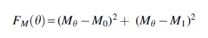
where ϴ is any threshold at which the function is being evaluated and M refers to the graph metric being used, with M_ϴ denoting the value of M evaluated on a graph that has been binarized using threshold ϴ and M ₀, M ₁ denoting the values of M at the extreme thresholds.

Each threshold is taken from the threshold space T_M of thresholds tested, ranging in steps of ɛ defined by the rounded rank threshold space from ϴ ₀ = kɛ to ϴ ₁ = Kɛ, for integers k < K, such that the boundary thresholds ϴ ₀, ϴ ₁ are both in the interval [0,1]. As noted earlier, ϴ ₀ is selected as the lowest threshold that gives density <1, which for a sparse network is ϴ ₀ = 0. Moreover, we used the percolation threshold as the upper bound for our objective function calculation, although it is possible that larger choices of this bound (for which GCC <1) could also work well.

That is, for a connected graph, such as the graph obtained by thresholding with the percolation threshold, all nodes are in the GCC. From there, if edges are removed uniformly at random, there is typically a rather abrupt transition from a GCC that includes all nodes to a much smaller GCC (Newman, 2001). Hence, very different GCC sizes will result from small increases in the threshold above the percolation threshold, and thus we would end up with similar ϴ ₁ values by selecting the smallest threshold such that the proportion of nodes in the GCC is ≥x% for any choice of x between 100 and some much smaller values (∼20 in our empirical explorations).

For biological networks that are known to comprise multiple components, a larger choice of ϴ ₁ than the percolation threshold would clearly be appropriate, but such networks are not considered in the simulation.

Optimization of OFT

We define the optimal threshold based on a given graph metric, M, from within the threshold space T_M , based on the values of the objective function F_M (ϴ) evaluated for all ϴ∊T_M . Specifically, we select the optimal threshold as the value at which F_M (ϴ) has an extremum on the interval [ϴ ₀, ϴ ₁]. This criterion selects the threshold at which the value of F_M is farthest from its end-point values.

Heuristically, this selection is based on the idea that at a sufficiently low threshold, weak edges are prevalent in the graph, to an extent that will likely have a strong influence on graph metric values. At a sufficiently high threshold, the network will have split (GCC <1) or be on the verge of splitting (GCC = 1) into disconnected components, which likely corresponds to meaningful edges having been discarded, and is also likely to have a strong influence on graph metrics. Thus, a useful threshold would be one for which the graph metric of interest deviates significantly from its values at these end-points.

In practice, we find that either M_ϴ rises from a low value at or near 0 at ϴ ₀, has an interior maximum, and then declines back to near 0 again at ϴ ₁, or else M _ϴ varies monotonically as ϴ increases from ϴ ₀ to ϴ ₁. In the former scenario, the optimal threshold is simply the threshold in (ϴ ₀, ϴ ₁) where the maximum of F_M (ϴ) occurs. In the latter case, we have F_M (ϴ₀ ) = F_M (ϴ ₁) = (M ₀ − M ₁)². At the same time, if F_M (ϴ) is monotonically increasing from ϴ ₀ to ϴ ₁, then for any ϴ∊ (ϴ ₀, ϴ ₁), M ₀ < M_ϴ < M ₁, and by the triangle inequality: $F_{M} (θ) = {(M_{θ} - M_{0})}^{2} + {(M_{θ} - M_{1})}^{2} \leq {(M_{θ} - M_{0} + M_{1} - M_{θ})}^{2} = {(M_{0} - M_{1})}^{2} .$

That is, F_M (ϴ) takes its maximal values at ϴ ₀ and ϴ ₁ and has an interior minimum between these extremes, at the ϴ value where M_ϴ = (M ₀ + M ₁)/2. A similar argument applies and gives an interior local minimum of F_M (ϴ) at the analogous ϴ value if M_ϴ is monotonically decreasing from ϴ ₀ to ϴ ₁.

Statistical threshold

Statistical thresholding involves retaining edges based on statistical significance and excluding edges that are not statistically significant (Bullmore and Bassett, 2011). We used a nominal uncorrected cutoff p < 0.05 to determine whether a correlational edge should be included in the binary network or not. The statistical threshold can be considered as a combinatorial thresholding technique, because it can remove edges that have a higher weight than some other edges it does not prune.

Maximum spanning tree

Kruskal's Algorithm (Kruskal, 1956), as implemented in a MATLAB package (Li, 2022), was used to determine the MST, which is defined as the smallest subset of edges in a graph that connects all nodes (GCC = 1); specifically, this algorithm selects the spanning tree with the heaviest weighted edges possible, hence the nomenclature MST. Notably, while the MST for a graph is fully connected (GCC = 1), unlike the percolation threshold that also yields a network for which the GCC = 1, the MST does not include any redundant edges.

Therefore, the MST thresholding method can be considered a combinatorial threshold because edges may be removed that are higher-weighted than other lower-weighted edges that are not removed.

Normalized mutual information

The NMI was calculated in previous publications as an evaluation criterion (Alexander-Bloch et al., 2012). Briefly, the NMI is a value between 0 and 1 that rates the similarity of two arbitrary lists of the same length, with 0 indicating completely chance correspondence, and 1 indicating perfect correspondence. The NMI values near 0 represent limited shared information, whereas values near 1 represent substantial shared information.

We compared two groupings of nodes into modules: that of the “ground truth” modular community structure for the LFR network, and that of each simulated FC after thresholding. The NMI thus quantifies the extent to which the module assignments for the nodes in each thresholded simulated FC agree with the nodes' assignments in the LFR network.

Empirical data

Empirical FCs were derived from the UK Biobank, a biomedical database containing lifestyle and health data on more than 500,000 participants (Miller et al., 2016). One hundred randomly selected participants without history of psychosis were examined to match the simulation sample size, a randomly selected subsample of a larger dataset with magnetic resonance imaging (MRI) data (n > 1400) that is being analyzed for a different project.

Networks were created using MATLAB on the Pittsburgh Supercomputing Center's (PSC) Bridges-2 system (Buitrago and Nystrom, 2021) using FreeSurfer (Fischl, 2012) and FSL (Jenkinson et al., 2012). Image acquisition parameters in the UK Biobank are published elsewhere (Smith et al., 2020).

Anatomical image processing

The UK Biobank images were processed for gradient distortion correction, brain extraction, and bias correction by the UK Biobank (Smith et al., 2020). T1w images were processed using the recon-all function from the FreeSurfer 7.2.0 via the official Dockerized image, using Singularity Image Format.

Then, each individual brain was parcellated according to the first Human Connectome Project Multi-Modal Parcellation (HCP MMP1) atlas (Glasser et al., 2016), using the Neurolab (2017) method. Briefly, this method uses an fs_average version of the HCP MMP1 parcellation (Mills, 2016) to map the atlas to the individual result of recon-all.

This produces the standard 360-node HCP MMP1 parcellation (180 parcels per hemisphere), including right and left hippocampus, plus 19 subcortical structures. Since the left and right substantia nigra (subcortical structures) are too small to be reliably parcellated using the Freesurfer automated segmentation, 17 subcortical structures are used, resulting in a total of 377 network nodes.

fMRI image processing and FC creation

Resting-state fMRI images were preprocessed by the UK Biobank (Smith et al., 2020) for head motion (MCFLIRT) (Jenkinson et al., 2012), grand-mean intensity normalization of each four-dimensional (4D) dataset, high-pass temporal filtering, echo-planar imaging unwarping and gradient distortion correction, and finally independent component anaylsis (ICA) denoising (Beckmann and Smith, 2004; Griffanti et al., 2014; Salimi-Khorshidi et al., 2014). The native T1 space brain was registered to the fMRI space using FSL FLIRT linear interpolation.

The resulting transform matrix used to register the anatomical atlas to the fMRI was then applied to the atlas parcellation image using nearest-neighbor interpolation to provide an fMRI-space anatomical atlas. This registration step was then quality controlled by visual inspection (2.5% of registrations were unsuccessful in the larger dataset).

The MRI data of 100 participants that passed the quality control were selected for this study. Finally, the spatially averaged time series across all voxels in a parcel was then calculated for each node, and the temporal correlations of nodal time series (Pearson's correlation) were then determined for each node pair, resulting in a resting-state FC.

Results

Negative FC simulation weights likely indicate noise

We generated ground truth LFR benchmark networks to represent baseline networks with nonnegative edge weights, with a predetermined modular structure, reminiscent of human brain SC networks. We then applied fMRI-like noise independently across 100 trials, resulting in simulated FC networks. Importantly, these simulated FC networks are perturbations of the benchmark LFR networks, where all edge weights are non-zero, and there are edges with negative weights.

In the simulated FC network, out of 65,703 possible edges in the off-diagonal, 4082 were non-zero in the LFR network, that is, dyadically connected in the LFR. Here, 661 of these 4082 (16%) were negatively weighted in the simulated FC network. On average, 26,740 FC simulation network weights were negative, indicating that a randomly selected negatively weighted edge in the simulated FC network had a 2.5% chance (661/26,703) of representing a true positive. The relationship between edge weights in the LFR and simulated FC network is shown in Figure 4.

FIG. 4.

The edgewise relationship between the ground-truth LFR edge weight (x-axis) and the population minimum of the corresponding FC_sim (FC_sim in the figure) edge is plotted. We chose to use the population minimum, rather than average, to depict a “maximally negative” scenario. Approximately 60% of the edges in the network are positive when considering the population minimum of each edge, and only 2.5% of negative edges in the simulated FC represent non-zero LFR edges.

Since negatively weighted edges are more likely to indicate a false positive (97.5% chance) than a true positive (2.5% chance), we reasoned that it is reasonable to zero-out the negatively weighted FC simulation network edges. Another common approach is to apply the absolute value function to the negative edges, thus ensuring that strongly negative edges are preserved.

We found that the absolute value approach will also preserve many false positives, which are the strongly negative FC simulation network edges appearing along the y-axis (Fig. 4). Since both removing negative edge weights and applying absolute value to them are acceptable solutions to apply to real FC data, we generated two downstream copies for each FC simulation network, one with negative weights zeroed out, and another with the absolute value function applied to the weights.

OFT with GCC = 1 selects lower threshold than percolation method

When considering the threshold values themselves, the OFT (using λ) and a GCC = 1 for the M ₁ parameter produced a significantly smaller threshold than the percolation method (t = 24.9, p < 0.0001 for both absolute value; negatives zeroed out, t = 224.2, p < 0.0001) (Fig. 5).

FIG. 5.

Histograms of the thresholds selected by the percolation threshold and objective thresholding methods. N = 100 for each histogram, two histograms shown per panel. (A) Using absolute value, the average threshold for the objective function was 0.26 (SD = 0.024) and for the percolation method the average threshold was 0.37 (SD = 0.023). (B) When zeroing out the negative, the average threshold for the objective function was 0.26 (SD = 0.028) and for the percolation method the average threshold was 0.37 (SD = 0.025). SD, standard deviation.

OFT yields relatively accurate modular structure

We applied statistical, percolation, and MST thresholding methods to each simulated FC network to generate binarized networks. For the OFT, we considered several graph metrics as in previous work and found that λ outperformed all other choices, including density, Q, average CC, efficiency, and assortativity, so we henceforth focus on results based on λ (Fig. 3).

We computed the NMI between LFR community assignments, and the module assignments calculated in the simulated FC network before and after thresholding and found that the OFT based on λ yielded the most accurate representation of the modular structure before and after removing the negative edges (Fig. 6).

FIG. 6.

Community NMI accuracy showing objective function thresholding producing more accurate modular structure. The NMI is a quantity between 0 and 1, where 0 represents no information is shared (in a sense, zero correlation) and 1 represents perfect information sharing. Bar heights represent population average NMI (across N = 100 replicates), and error bars represent SDs.

The OFT yielded the highest NMI in terms of average NMI of detected modules after thresholding to the ground truth LFR module structure, regardless of how negative weights were handled. All differences were significant, between any choice of comparisons, except for the two MST outputs (both average NMI 0.482). Although the percolation threshold and OFT applied to absolute values of correlations appear numerically close, the difference was statistically significant (t = 6.46, p < 0.0001). Likewise, when negative edges are set to zero, the OFT yields a higher NMI than the percolation threshold (t = 11.28, p < 0.0001).

OFT yields relatively accurate CC and density

Whereas NMI provides a quantitative basis for community similarity, or network organization, density provides a more straightforward perspective regarding whether the correct number of edges were removed (Fig. 7). Accuracy is defined as thresholded network density minus the density of the ground truth LFR network. A density accuracy of 0 indicates that the binarization perfectly restored network density (though not necessarily by removing the correct edges).

FIG. 7.

Comparison of thresholding methods for accuracy of density. Since the LFR ground truth density is subtracted from the FC_sim (FC_sim in the figure) density at each replicate, negative density accuracy values indicate that the binarization method removed too many edges, and positive accuracy values indicate that not enough edges were removed. All differences are significant. Bar heights represent population (N = 100 replicates) averages, and error bars represent SDs. The maximum spanning tree has no error bars because the number of edges in the maximum spanning tree is a function of the number of nodes in the network and does not vary by replicate.

A negative accuracy value indicates that too many edges were pruned, and a positive accuracy value indicates that not enough edges were pruned. The LFR network had a density of 0.0621. The MST (where density does not differ by simulation replicate) has a density of 0.0055, indicating that the LFR network has about 11 times as many edges as its MST. The FC simulation network with negatives zeroed out has a density of 0.581, indicating that 41.9% of FC simulation network edges are, on average, negatively valued.

The density of any FC simulation network after taking the absolute value but before thresholding would always be 1. The percolation threshold and OFT yielded density accuracy values with much smaller magnitude, with the smallest magnitudes associated with the OFT; moreover, even the closest two unequal values, derived using the percolation threshold with absolute values and OFT with absolute values are statistically significantly different (t = 38.3, p < 0.0001).

The CC on a nodal basis represents the degree to which a node's neighbors are connected to each other. Thus, the CC of MST is 0 for all nodes. The nodal average CC of the LFR network is 0.431. We defined a CC accuracy by first subtracting the LFR CC value for each node from each individual FC simulation network replicate's CC value for that node, then averaging the nodal accuracies across the population of replicates, and finally computing the global average over all nodes (Fig. 8). Again, the OFT significantly outperforms other thresholding methods even in the absolute value condition where the outcomes are closest (t = −10.09, p < 0.0001).

FIG. 8.

Comparison of thresholding methods for accuracy of CC. The LFR ground truth nodal CC is subtracted from the FC_sim (FC_sim in the figure) nodal CC at each replicate, then these nodal CC accuracies are averaged across the population, and finally “global” CC accuracy is calculated by averaging over nodal CCs. This means that negative CC accuracy values indicate that the binarization method produced nodal CC values that are, on average, lower than the nodal average CC of the LFR, and positive CC accuracy values indicate that the global CC of the binary network is higher than the global CC of the LFR. The global CC (the average of the nodal CCs) for the LFR network was 0.431. The maximum spanning tree CC accuracy has error bars, because the nodes within the LFR do not have uniform CC. All differences are significant, including the differences between statistical thresholding and zeroing negatives. Bar heights represent global CC accuracy after averaging across all 100 replicates, and error bars represent SDs.

Application to empirical data

While there is no absolute ground truth for modularity of empirical data, FC created from 100 UK Biobank subjects using the HCP atlas were compared with the proposed modularity of the HCP atlas (Glasser et al., 2016) (neuroanatomical supplement) (Fig. 9). The NMI between the weighted networks and the ground truth was 0.184, which improved significantly (t = 2.61, p < 0.01) to 0.203 when anti-correlated edges (20% ± 7%) were removed.

FIG. 9.

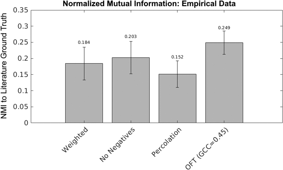
The NMI between the Glasser parcellation proposed “ground truth” community membership of atlas regions and the binarized networks compared for: full weighted networks, “no negative” networks, percolation thresholded networks with no negatives, and OFT weighted networks with no negatives for GCC minimum for M ₁ = 45%. Error bars represent SDs. OFT, objective function threshold.

The NMI between literature ground-truth and empirical networks was significantly worse (t = 4.95 p < 0.0001) when weighted networks were binarized with the percolation threshold (NMI = 0.152) compared with the original weighted networks (NMI = 0.184). Finally, when the GCC was optimized (GCC = 45%), the maximum NMI between the binarized networks using the OFT (NMI = 0.249) was significantly better than both the binary percolation thresholded networks (t = 17.63, p < 0.0001) and the original weighted networks (t = 10.34 p < 0.0001).

The mean threshold selected for the percolation threshold was 0.12 ± 0.022, and for the OFT 0.56 ± 0.118. The average number of modules detected using the percolation threshold was 2.23 ± 0.584, and for the OFT 5.93 ± 3.611.

Discussion

Thresholding, a form of binarization, is often a critical step in network analysis with important downstream consequences. We compared several existing thresholding methods and noted drawbacks in applying these methods in some settings. To address these drawbacks, we developed the OFT method that can be implemented using any graph metric (Fig. 2). We applied OFT and other thresholding methods to simulated FC networks derived from a ground truth LFR network to compare the performance of these methods in silico (Fig. 1).

Our method is “objective” both mathematically and semantically. That is, mathematical optimization is the process of finding an extremum of a function known as a cost function or objective function, which is exactly what we do to arrive at an optimal threshold value; semantically, our method objectively determines the threshold by an automated procedure, without the need for subjective judgments in the process. The objective function that we use quantifies the difference between any scalar graph metric defined across a range of thresholds and its values at both end-points of the threshold range, based on the idea that the low threshold end-point represents an overly dense network due to the preservation of edges representing low signal and high noise, while the high threshold end-point corresponds to an overly sparse network that lacks the redundancy characteristic of brain connectivity.

We evaluated the OFT method for a set of graph metrics (density, λ, efficiency, CC, modularity, and assortativity) and found that λ was the best performing choice of metric (Fig. 3). Performance was defined by the NMI between the network modules detected after binarization of simulated FC networks derived from a benchmark LFR network and the ground-truth modules associated with the benchmark LFR network itself (Fig. 1).

Comparing community partitions through NMI is a widely used approach that provides a reliable measure of network community structure similarity, robust to small changes in edge-wise network content (Danon et al., 2005; Lancichinetti et al., 2009). In this work, we have shown, based on NMI calculation (Fig. 6), that the OFT method better restored the original graph structure than did previously published threshold selection methods evaluated here, including the percolation (Bordier et al., 2017), statistical (Bullmore and Bassett, 2011), and MST (Kruskal, 1956; Li, 2022) thresholding.

This result held regardless of how negative values were treated in the simulated FC networks. Moreover, the OFT method produced node-wise CCs (Fig. 8) and graph densities (Fig. 7) that were closer to those of the baseline network than did the other thresholding approaches. Finally, when the GCC is limited to 100% of nodes, the OFT, by design, yielded the smallest threshold (Fig. 5), meaning that more edges were preserved.

The OFT method is simple to apply, because there are readily available software options for computing graph metrics. The method can be applied to any network, with any form of adjacency matrix. For example, unlike the percolation threshold, which can only be applied to path connected networks for which all nodes belong to the GCC, the objective function approach can be adapted to networks with smaller GCCs, say GCC = x, by setting the upper threshold to be the threshold at which GCC first drops to some value less than or equal to C_x where C is any number in the interval (0,1] and by choosing a graph metric that is well defined on networks that are not path connected.

We find that the OFT based on λ outperformed the other methods across all of these performance measures and thus offers an attractive approach to consider for thresholding of networks based on experimental or clinical measurements. We also show evidence that the OFT performs better than existing methods for thresholding in empirical data, depending on GCC choice (Fig. 9).

Given its intuitive underpinnings, ease of use, and superior performance in our simulation study, we conclude that the OFT method should receive serious consideration for use in thresholding in future studies of brain connectivity involving binarization of connectivity matrices.

One recent review found that “direct structural connectivity optimistically explains no more than 50%” of functional connectivity (Suarez et al., 2020), and that SC-FC edge-weight correlations range between R = 0.3–0.7. In future work, OFT could be used to re-examine the relation between SC and FC data obtained from individual subjects.

Such comparisons typically involve thresholding to deal with the very different types of values—non-negative integer counts of streamlines in the SC versus correlation values between −1 and 1 in the FC used to form networks across these two imaging modalities. As in our simulated FC data, it is challenging to handle negative values (Fig. 4).

For FC data, large negative values could be considered important, since negative correlations also represent relationships in the activity of two brain regions; hence, taking the absolute values of correlations before thresholding may be reasonable, the approach that we took in our study. Alternatively, the network can be partitioned into “negative edges only” and “positive edges only” subnetworks for separate analysis.

This may create networks with GCC <1, a condition that is allowed in the OFT method. An OFT could be derived for each of these subnetworks, whereas it is likely that at least one of these subnetworks would not be path connected, which would be problematic for other thresholding methods.

We used a quadratic objective function, which is a standard choice that avoids issues of cancellation of terms of opposite signs and provides smoothness. Other functional forms could be considered, however. In the case where M_ϴ is monotone, the interior extremum of F_M (ϴ) occurs at the ϴ value where M_ϴ = (M ₀ + M ₁)/2. In theory, if a practitioner had additional knowledge suggesting that the network of important edges in a dataset was in some sense more similar to M ₀ than to M ₁, or vice versa, then the weights in this average could be adjusted to yield an optimal threshold ϴ where M_ϴ = aM ₀ + bM ₁ for some choice of constants a, b satisfying a + b = 1 other than (1/2, 1/2).

Conclusions

Network thresholding plays a crucial, early role in the overall process of seeking to understand the relationships encoded in brain connectivity networks. Ideally, threshold selection would be done via an automated procedure based on easily calculable quantities, to allow for reproducibility and reduce bias. The OFT method that we have proposed provides such a procedure, which can be flexibly adapted to reflect knowledge about the underlying network before it is applied, and hence represents a useful addition to our toolbox for brain network analysis.

Footnotes

Authors' Contributions

N.T., J.R., and K.M.P. conceived the concept. N.T. conducted the analyses under the supervision of J.R., S.I., J.C., and K.M.P. N.T., J.R., and K.M.P. drafted the manuscript. S.I. and J.C. reviewed and edited the manuscript. All authors approved the manuscript.

Author Disclosure Statement

None of the authors have any conflict of interest specific to this publication.

Funding Information

This work was funded through grants from the US National Institute of Mental Health (NIMH; R01MH112584 and R01MH115026; K.M.P.). The funding agency did not influence the contents of the manuscript.

References

Alexander-Bloch

, Lambiotte

, Roberts

, et al. The discovery of population differences in network community structure: New methods and applications to brain functional networks in schizophrenia. Neuroimage, 2012; 59(4):3889–3900; doi: 10.1016/j.neuroimage.2011.11.035

Bassett

, Bullmore

, Verchinski

, et al. Hierarchical organization of human cortical networks in health and schizophrenia. J Neurosci, 2008; 28(37):9239–9248; doi: 10.1523/JNEUROSCI.1929-08.2008

Beckmann

, Smith

. Probabilistic independent component analysis for functional magnetic resonance imaging. IEEE Trans Med Imaging, 2004; 23(2):137–152; doi: 10.1109/TMI.2003.822821

Bordier

, Nicolini

, Bifone

. Graph analysis and modularity of brain functional connectivity networks: Searching for the optimal threshold. Front Neurosci, 2017; 11:441; doi: 10.3389/fnins.2017.00441

Buitrago

, Nicholas

. Neocortex and Bridges-2: A High Performance AI+HPC Ecosystem for Science, Discovery, and Societal Good. In: High Performance Computing ( Nesmachnow

, Castro

, Tchernykh

. eds.) Springer International Publishing: Cham; 2021; pp. 205–219.

Bullmore

, Bassett

. Brain graphs: Graphical models of the human brain connectome. Annu Rev Clin Psychol, 2011; 7:113–140; doi: 10.1146/annurev-clinpsy-040510-143934

Chen

, He

, Rosa-Neto

, et al. Revealing modular architecture of human brain structural networks by using cortical thickness from MRI. Cereb Cortex, 2008; 18(10):2374–2381; doi: 10.1093/cercor/bhn003

Danon

, Diaz-Guilera

, Duch

, et al. Comparing community structure identification. J Stat Mech, 2005; 9:P09008; doi: 10.4855/0/arXiv.cond-mat/0505245

Drakesmith

, Caeyenberghs

, Dutt

, et al. Overcoming the effects of false positives and threshold bias in graph theoretical analysis of neuroimaging data. Neuroimage, 2015; 118:313–333.

10.

Ferrarini

, Veer

, Baerends

, et al. Hierarchical functional modularity in the resting-state human brain. Hum Brain Mapp, 2009; 30(7):2220–2231.

11.

Fischl

. FreeSurfer. Neuroimage, 2012; 62(2):774–781; doi: 10.1016/j.neuroimage.2012.01.021

12.

Glasser

, Coalson

, Robinson

, et al. A multi-modal parcellation of human cerebral cortex. Nature, 2016; 536(7615):171–178; doi: 10.1038/nature18933

13.

Griffanti

, Salimi-Khorshidi

, Beckmann

, et al. ICA-based artefact removal and accelerated fMRI acquisition for improved resting state network imaging. NeuroImage, 2014; 95:232–247.

14.

Jenkinson

, Beckmann

, Behrens

, et al. Fsl. Neuroimage, 2012; 62(2):782–790; doi: 10.1016/j.neuroimage.2011.09.015

15.

Kruskal

. On the shortest spanning subtree of a graph and the traveling salesman problem. Proc Am Math Soc, 1956; 7(1):48–50; doi: 10.1090/S0002-9939-1956-0078686-7

16.

Lancichinetti

, Fortunato

, Kertész

. Detecting the overlapping and hierarchical community structure in complex networks. New J Phys, 2009; 11(3):033015; doi: 10.1088/1367-2630/11/3/033015

17.

Lancichinetti

, Fortunato

, Radicchi

. Benchmark graphs for testing community detection algorithms. Phys Rev E Stat Nonlin Soft Matter Phys, 2008; 78(4 Pt 2):046110.

18.

. Maximum Weight Spanning Tree (Undirected). MATLAB Central File Exchange; 2022. Available from: https://www.mathworks.com/matlabcentral/fileexchange/23276-maximum-weight-spanning-tree-undirected [Last accessed: September 6, 2022 ].

19.

Miller

, Alfaro-Almagro

, Bangerter

, et al. Multimodal population brain imaging in the UK Biobank prospective epidemiological study. Nat Neurosci, 2016; 19(11):1523–1536.

20.

Mills

. HCP-MMP1.0 projected on fsaverage; Figshare. Dataset, 2016. Available from: https://doi.org/10.6084/m9.figshare.3498446.v2 [Last accessed: May 26, 2022 ].

21.

Neurolab

. HCP-MMP1.0 volumetric (NIfTI) masks in native structural space; figshare. Dataset, 2018. Available from: https://doi.org/10.6084/m9.figshare.4249400.v5 [Last accessed: May 26, 2022 ].

22.

Newman

LS.

What Is Social Cognition? Four Basic Approaches and Their Implications for Schizophrenia Research. In: Social Cognition and Schizophrenia. ( Corrigan

, Penn

. eds.) American Psychological Association: Washington, DC, 2001; pp. 41–72.

23.

Newman

. Modularity and community structure in networks. Proc Natl Acad Sci U S A, 2006; 103(23):8577–8582; doi: 10.1073/pnas.0601602103

24.

, Wang

, Yu

, et al. Discriminative structure feature engineering for macroscale brain connectomes. IEEE Trans Med Imaging, 2015; 32(11):2333–2342.

25.

Rubinov

, Sporns

. Complex network measures of brain connectivity: Uses and interpretations. Neuroimage, 2010; 52(3):1059–1069; doi: 10.1016/j.neuroimage.2009.10.003

26.

Salimi-Khorshidi

, Douaud

, Beckmann

, et al. Automatic denoising of functional MRI data: Combining independent component analysis and hierarchical fusion of classifiers. Neuroimage:, 2014; 90:449–468.

27.

Smith

, Alfaro-Almagro

, Miller

. UK Biobank Brain Imaging Documentation. Wellcome Centre for Integrative Neuroimaging (WIN-FMRIB), Oxford University on behalf of UK Biobank; 2020. Available from: https://biobank.ctsu.ox.ac.uk/crystal/ukb/docs/brain_mri.pdf [Last accessed: May 24, 2015 ].

28.

Sotiropoulos

, Zalesky

. Building connectomes using diffusion MRI: Why, how and but. NMR Biomed, 2019; 32(4):e3752; doi: 10.1002/nbm.3752

29.

Suarez

, Markello

, Betzel

, et al. Linking structure and function in macroscale brain networks. Trends Cogn Sci, 2020; 24(4):302–315; doi: 10.1016/j.tics.2020.01.008

30.

van den Heuvel

, de Lange

, Zalesky

, et al. Proportional thresholding in resting-state fMRI functional connectivity networks and consequences for patient-control connectome studies: Issues and recommendations. Neuroimage:, 2017; 152:437–449.

31.

Welvaert

, Durnez

, Moerkerke

, et al. neuRosim: An R package for generating fMRI data. J Stat Softw, 2011; 44:1–18.

32.

Zanin

, Sousa

, Papo

, et al. Optimizing functional network representation of multivariate time series. Sci Rep, 2012; 2:630.