Atlas-Based Labeling of Resting-State fMRI

Abstract

Background:

Functional magnetic resonance imaging (fMRI) has the potential to provide noninvasive functional mapping of the brain with high spatial and temporal resolution. However, fMRI independent components (ICs) must be manually inspected, selected, and interpreted, requiring time and expertise. We propose a novel approach for automated labeling of fMRI ICs by establishing their characteristic spatio-functional relationship.

Methods:

The approach identifies 9 resting-state networks and 45 ICs and generates a functional activation feature map that quantifies the spatial distribution, relative to an anatomical labeled atlas, of the z-scores of each IC across a cohort of 176 subjects. The cosine-similarity metric was used to classify unlabeled ICs based on the similarity to the spatial distribution of activation with the pregenerated feature map. The approach was tested on three fMRI datasets from the 1000 functional connectome projects, consisting of 280 subjects, that were not included in feature map generation.

Results:

The results demonstrate the effectiveness of the approach in classifying ICs based on their spatial features with an accuracy of better than 95%.

Conclusions:

The approach significantly reduces expert time and computation time required for labeling ICs, while improving reliability and accuracy. The spatio-functional relationship also provides an explainable relationship between the functional activation and the anatomically defined regions.

Impact Statement

Resting-state functional magnetic resonance imaging labeling using anatomical atlas matching streamlines the process of automatically labeling brain networks through learned spatial representations. By aligning the functional connectivity patterns obtained through independent component analysis (ICA) with anatomical atlases, this method allows for the automatic assignment of labels to the components/networks based on assessing the distribution of the strength of signals across regions. Through this approach, researchers can efficiently identify and interpret the various components extracted via ICA, enhancing our understanding of the brain’s intrinsic connectivity architecture with minimal manual intervention.

Introduction

Resting-state functional magnetic resonance imaging (rs-fMRI) (Smith et al., 2013) is a reliable technique for brain mapping and precise localization of various brain networks without the need for explicit task performance. Independent component analysis (ICA) (Calhoun and Adali, 2006) is a popular analysis method to decompose rs-fMRI signals into functional network maps by separating independent blood oxygen level dependent (BOLD) signals into individual components based on distinctions of time courses among different components, including networks and noise-related signals. However, conventional labeling of ICA components requires visual identification of networks by at least one experienced neuroimager, which can lead to bias and inter-observer errors. To improve reliability, more than one neuroimager usually reviews the components, but this method is limited to small-scale datasets and may still be prone to inter-expert variability.

To address these limitations, researchers have focused on developing automated methods for identifying and labeling neural networks in healthy and brain tumor patients. Initial attempts for developing the Holistic Atlases of Functional Networks and Interactions (Lv et al., 2015) faced multiple challenges for automatic recognition of resting state networks (RSNs) owing to the lack of functional brain atlases, susceptibility to noise, and loss of accuracy in large datasets.

Most initial studies classified the problem into identifying noise versus useful components of subsequent noise or artifact removal. Tohka et al. (2008) automatically detected components clearly relating to artifacts or noise by training a global decision tree classifier on 20 subjects and testing on 12 subjects. Six features for the classifier were derived and a mis-classification rate of 0.214 and 0.26 was calculated. In 2013, Bhaganagarapu et al. (2013) analyzed the individual ICA on 50 rs-fMRI subjects. They created a spatially organized component klassifikator to distinguish between ICs dominated by noise and those dominated by possible neuronal signals. Only 0.3% of the ICs differed from the manually identified artifacts. Then in 2020, Tassi et al. (2020) created a semi-automated classification method to identify and remove fMRI noise based on spectral power and spatial correlations. The tool was tested on five subjects and was found to be 80% accurate in distinguishing noise-related ICs from non-noise.

Spatial-based IC classification gives more information to distinguish ICs in resting-state fMRI data. De Martino et al. (2007) developed a new fMRI classification algorithm that can be used to automatically label fMRI components. The algorithm works by first associating each fMRI component with an IC-fingerprint, a multidimensional representation of descriptive measures of the component. The IC-fingerprint is then used to classify the component into one of six general classes using a support vector machine (SVM) classifier. The algorithm was able to correctly label 94% of the components and 100% of the task-related components. Vergun et al. (2016) used ICA and machine learning to classify RSNs in 23 epilepsy patients and 30 healthy subjects. The researchers compared decision trees, perceptrons, naïve Bayes classifiers, and SVMs. The best results were obtained with a naïve Bayes classifier, which achieved an accuracy of 88% for epilepsy patients and 90% for healthy subjects. Doucet et al. (2011) used a fully unsupervised classifier to classify RSNs in 180 subjects. The researchers compared the ICA maps z-score overlaps to determine the correlated ICs. The classifier was able to successfully classify 91% of the ICs and recover 34 RSNs.

In 2018, Zhao et al. (2018) designed and evaluated a deep 3D convolution neural network (CNN) framework for automatic classification and recognition of whole-brain fMRI signals based on the Human Connectome Project fMRI data, which contained 68 subjects with 7 tasks and 1 resting-state fMRI. Their result demonstrated that the 3D CNN model could successfully recognize 10 RSNs. However, their data acquisition required manual labeling, which was time-consuming and prone to mislabels, highlighting the need for a fully- or semi-automated network labeling method. Nozais et al. (2021) proposed a deep learning approach to enable the automated classification of individual IC decompositions into a set of predefined RSNs. The researchers used the BIL&GIN dataset (Brain Imaging of Lateralization by the “Groupe d’Imagerie Neurofonctionelle”), which contains fMRI data from 282 subjects (Mazoyer et al., 2016). They used two algorithms to automatically cluster the ICs into 45 RSNs and trained an multilayer perceptron (MLP) on the fMRI data, using the 45 RSNs as the ground truth. The MLP was able to achieve a testing accuracy of 92% in RSN classification. Chou et al. (2022) used a Siamese network to learn discriminative feature representation for single-subject ICA component classification. They showed that the Siamese network out-performed a CNN network with over 99% accuracy on an outside dataset.

In light of the requirement for more precise labeling of ICs on a larger scale, we have developed a new approach in this study that utilizes the spatial correlation between an anatomical atlas of the brain and the functional RSNs in fMRI of healthy subjects. We used cosine similarity to predict and label ICA components based on the IC activation defined in a publicly available standard anatomical atlas (Harvard-Oxford cortical structural atlas), which covers 48 cortical and 21 subcortical structural areas. Finally, we tested the labeling method on a subset of 280 subjects from the 1000 Functional Connectomes Project, including four geographically different cohorts to evaluate the accuracy, sensitivity, and specificity of our model in predicting and labeling the ICA components and RSNs.

Materials and Methods

This retrospective study used deidentified publicly available data, compatible with the Health Insurance Portability and Accountability Act, and therefore was considered nonhuman subject research with institutional review board review waived.

Experimental dataset

We employed a publicly available dataset from the 1000 Functional Connectomes Project (Biswal et al., 2010). This dataset comprises fMRI echo planar acquisitions obtained using a 3T scanner with a repetition time (TR) of approximately 2 s as well as T1-weighted images of four distinct cohorts based on the regions of acquisition. These cohorts include Beijing_Zang (n = 198, 76M/122F, mean age = 21.2), NewYork_a (n = 84, 43M/41F, mean age = 24.4), Bangor (n = 20, 20M/0F, mean age = 23.4), and PaloAlto (n = 17, 2M/15F, mean age = 32.5). We excluded 22, 4, and 13 subjects from the Beijing_Zang, NewYork_a, and Bangor cohorts, respectively, due to misalignment errors during coregistration.

fMRI preprocessing/group ICA

The fMRI volumes underwent slice timing correction followed by motion correction using Functional Magnetic Resonance Imaging of the Brain’s Linear Image Registration Tool or MCFLIRT, as implemented in FSL (Jenkinson et al., 2012). The data was affine-registered to the standard Montreal Neurological Institute (MNI-152) space (Mazziotta et al., 2001) using FMRIB’s Linear Image Registration Tool (FLIRT). Group ICA (GICA) (Abou Elseoud et al., 2011; Du and Fan, 2013) was performed on fMRI scans using temporal concatenation approach by Multivariate Exploratory Linear Optimized Decomposition into Independent Components (MELODIC) (Beckmann, 2012) tool in Functional Magnetic Resonance Imaging of the Brain Software Library 6.0 or FSL (Functional Magnetic Resonance Imaging of the Brain Analysis Group) with default parameters. The MELODIC model order was set to 100 ICs. GICA output ICs were reviewed, in no specific order, and labeled by a neuroradiologist with 15 years of fMRI experience. To label each IC, the neuroradiologist analyzed: 1) the spatial map, 2) the time course, and 3) the power spectrum of the time course. ICA maps with dominant signal outside the brain parenchyma and in white matter were classified as noise; for signals within the brain parenchyma, components were classified as noise if the time courses were of high frequency with very narrow power spectrum (i.e., very regular, for example, those that can be related to vasculature aliasing into brain) or very broad power spectrum. For the remainder of non-noise components, the location of the dominant cluster or clusters and the pattern of nondominant clusters were utilized to classify the component into intrinsic brain networks. The labels are shown in the Supplement along with the correspondence to the universal taxonomy (Uddin et al., 2019). We used a dual regression algorithm implemented in FSL to identify the subject-specific spatial and temporal dynamics against the original data and to estimate group components per subject.

Anatomical atlas

In our study, we utilized the Harvard-Oxford cortical and subcortical structural atlas (Desikan et al., 2006) as a standard MNI template to accurately localize the ICA spatial map to specific anatomical regions of the brain. This atlas was derived from structural data and segmentations of T1-weighted images of 21 healthy male and 16 healthy female subjects, ages 18–50 years, provided by the Harvard Center for Morphometric Analysis covering 48 cortical and 21 subcortical structural areas. To further improve the spatial accuracy, we split labeled regions that crossed the midline into left and right versions, resulting in a total of 76 anatomical labels. The use of this atlas allowed for a more precise and standardized interpretation of the ICA spatial map, enabling us to investigate the functional connectivity of specific brain regions with greater accuracy and specificity.

Anatomical region—average contribution map

We used the Beijing Cohort to establish the relationship between anatomical regions and their functional activations. In total, 176 subjects were included from the Beijing Cohort, each of which had 45 ICs (excluding noise). Hence, there were 7920 ICs in the cohort.

To design the average activation map, we used a three-step approach:

Step 1: For each of the ICs, we calculated the mean z-score (Chou et al., 2022) within each of the 76 anatomical regions.

Step 2: Averaged the activation across all 176 volumes belonging to a single IC (e.g., Default Mode Network [DMN]-RSC, Motor-Dorsal-Hand) to obtain the cohort level mean functional activation of all 76 anatomical regions in one IC (1 × 76 vector).

Step 3: Repeated steps 1 and 2 for all 45 ICs. We obtained the functional activation distribution over anatomical regions for each IC, as shown in Table 1 (activation fingerprint) (45 × 76 matrix).

Table 1.

Labeling Accuracy, Sensitivity, and Specificity over All Four Cohorts within the Dataset

Data set (N)	Accuracy (%)	Sensitivity (%)	Specificity (%)
Beijing (176)	99.2	99.4	98.3
New York (80)	97.9	100	97.5
Palo Alto (17)	97.4	94.1	94.1
Bangor (7)	99.1	100	100
Average	98.4	98.4	97.5

This resulted in a functional–spatial relationship that relates the mean functional activation in each of the 76 anatomically labeled regions. This functional–spatial relationship provided a fingerprint that relates the spatial activation for each IC and further enabled a method to “look-up” an unlabeled activation distribution across the labeled regions to estimate the likely IC label. Figure 1 shows the T1 MRI scan (left) and the associated Harvard-Oxford Cortical atlas of the same slice (middle). An example of fMRI ICA component, DMN-RSC in this case, is shown (right) in the figure.

FIG. 1.

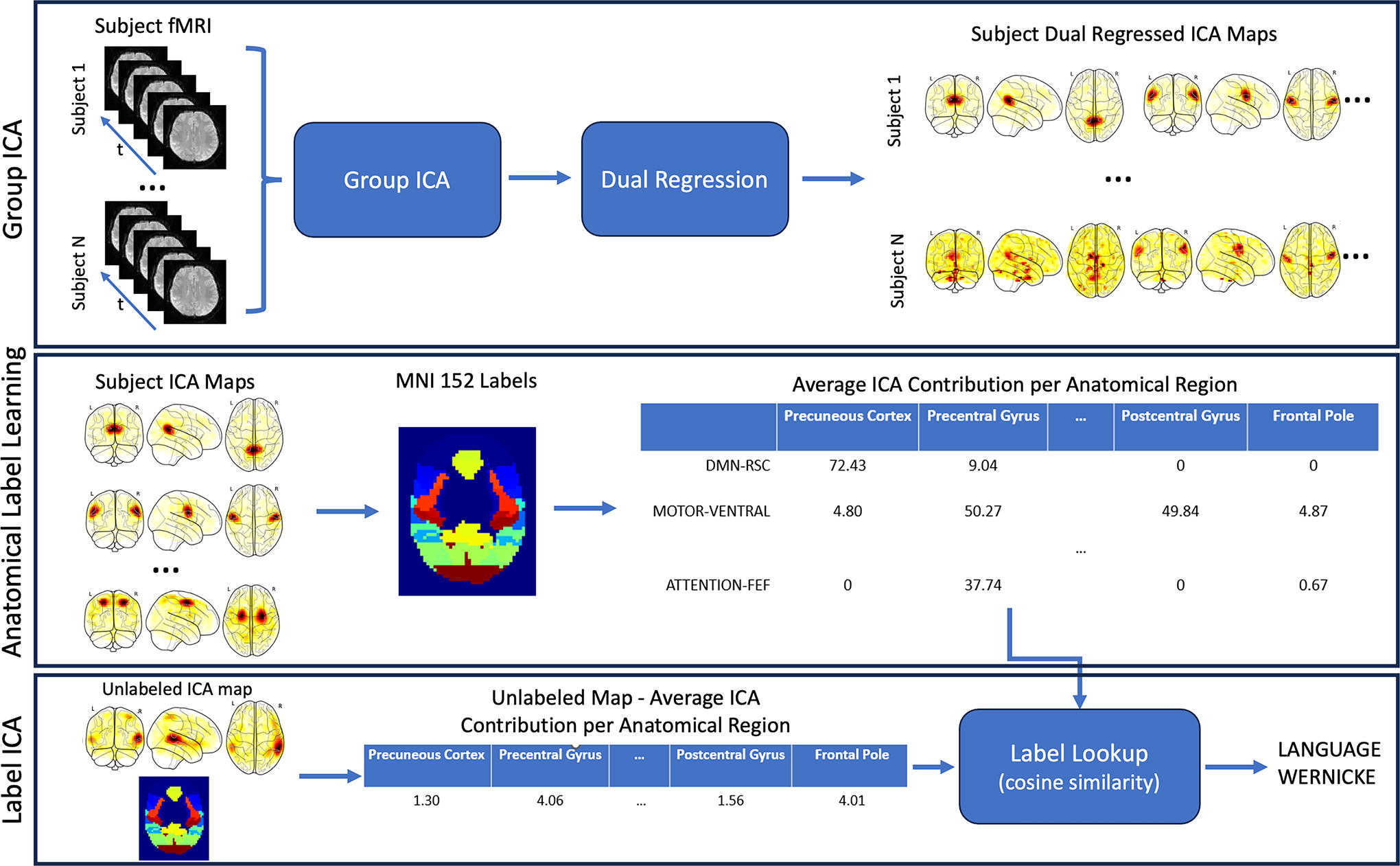
Outline of the GICA, anatomical label training, and label ICA lookup. GICA (top): Training data was processed using GICA and dual regression to create ICA maps for each subjects’ training data. Anatomical Label Learning (middle): The dual regressed ICA data were averaged within each anatomical label region of the Harvard-Oxford cortical atlas (training). Label ICA (top): the average ICA signal contribution is quantified per anatomical label and then compared to the table built in Anatomical Label Learning (inference). ICA, independent component analysis; group independent component analysis, GICA.

Label lookup

The cosine similarity was used to compute the similarity between a pair of feature vectors independent of the magnitude: $similarity = \cos (θ) = \frac{A \cdot B}{‖| | A | |‖ ‖| | B | |‖}$ (1)where A and B are the functional activation contributions over the anatomical regions (e.g., a row in Fig. 2 middle table). The smaller the angle formed between two feature vectors, the greater the similarity, and vice versa.

FIG. 2.

(a) MNI-152 space to which the T1-weighted MRI images are registered during preprocessing. (b) The anatomical labels created from splitting bilateral regions from the Harvard–Oxford cortical atlas. (c) A functional activation volume of DMN-RSC (slice 22, subject 100). MNI-152, Montreal Neurological Institute-152; MRI, magnetic resonance imaging; DMN, Default Mode Network.

Statistical testing

The test part of the Beijing dataset and three other sites (NewYork_a, Bangor, and PaloAlto) were used to assess the labeling accuracy. Each of the test sets were run through GICA as described in the aforementioned section and the functional activation ICs were computed. Each functional IC was compared to the Beijing training set. To label the IC, the mean IC was computed for each spatial region, and then that feature vector was compared with all the labeled features from the Beijing dataset. The labeled feature that corresponded best (highest similarity from Equation 1) was taken to be the correct label.

We grouped the ICs related to the nine RSN including DMN, Attention, Executive, Visual, Sensory, Salience, Language, Auditory, Motor-Dorsal-Hand. The metrics including accuracy, sensitivity, and specificity were calculated for IC levels and RSN levels for all four datasets.

Results

The average contribution map of the training Beijing Cohort on 76 anatomical regions (reference data set) in each of the 45 ICs is shown in Supplementary Table S1 (in the Appendix). Overall, the top three anatomical regions for each ICA were consistent with prior knowledge. Six examples of ICAs with the mean z-score for each atlas-based label region are shown in Figure 3. The atlas label mean z-score is distributed over the whole brain volume in a way consistent with prior knowledge.

FIG. 3.

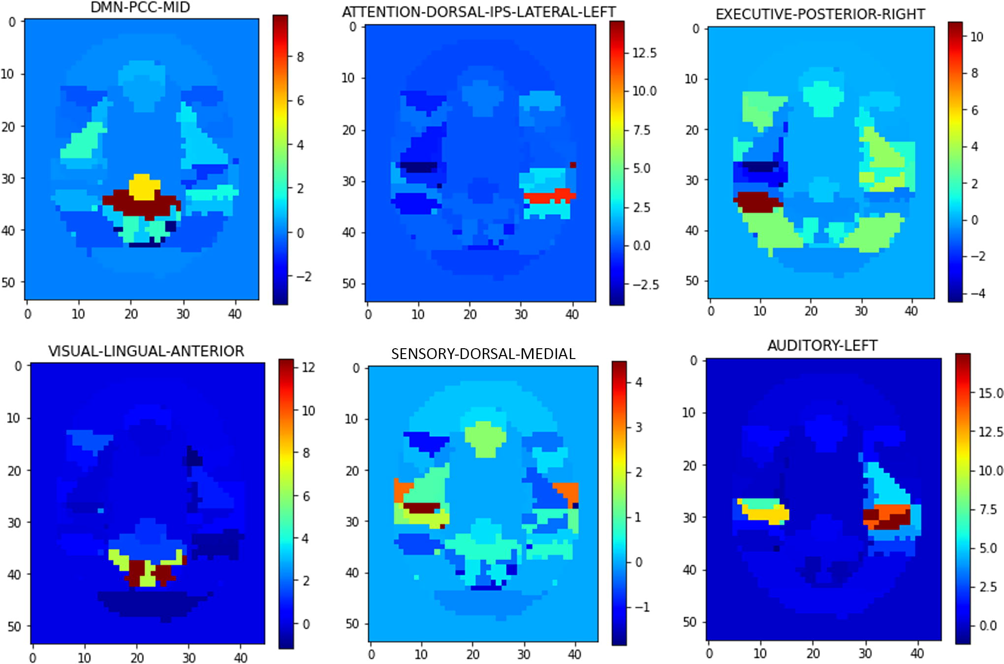
Example mean z-scores in atlas regions for six functional ICAs: DMN-PCC-MID, ATTENTION-DORSAL-IPS-LATERAL-LEFT, EXECUTIVE-POSTERIOR-RIGHT, VISUAL-LINGUAL-ANTERIOR SENSORY-DORSAL-MEDIAL, and AUDITORY-LEFT. ICA, independent component analysis; DMN, Default Mode Network.

Classification: IC level

Table 1 summarizes the accuracy, sensitivity, and specificity of the predictive power of the IC labels from each of the test sets (hold-out test set from Beijing cohort along with the New York, Palo Alto, and Bangor cohorts). The best results were seen in the Beijing hold-out test set, which is not unexpected, as the method was trained on the Beijing data. Although the accuracy in the three test datasets is lower than the Beijing dataset, they remained above 97% across all three other test datasets. The average accuracy of 95% was not unexpected as the ICA signal distribution across the brain regions is well localized to specific anatomical regions. The sensitivity and specificity of the three test datasets were above 94% for each cohort and overall they were better than 98% on average across the cohorts.

Classification: Network level

The network-level accuracy for each cohort test set is shown in Table 2. Overall, the network-level classification was 98.5% accurate across all networks. The network-level accuracy was 95% or better in all networks except the Motor network, which was 94.4% accurate.

Table 2.

Accuracy of Classification of Each Resting-State Network Component across All Four Test Cohorts: Hold-Out Test Set of Beijing, and the Full New York, Palo Alto, and Bangor Cohorts

	Accuracy (%)
Network	Beijing	New York	Palo Alto	Bangor	Average
DMN	98.8	98.7	98.0	98.8	98.6
ATTENTION	98.0	93.1	95.1	97.6	96.0
EXECUTIVE	100	100	100	100	100
VISUAL	99.8	99.4	99.4	100	99.6
SENSORY	99.2	97.1	96.1	100	98.1
SALIENCE	100	100	100	100	100
LANGUAGE	100	100	100	100	100
AUDITORY	100	100	100	100	100
MOTOR	98.4	94.4	88.2	96.4	94.4
			Overall Average		98.5

Missed classifications

Functional regions that localized close in space could lead to incorrect labeling. For example, DMN-PCC-Posterior and DMN-PCC-Anterior (Fig. 4) are distinct regions but close in atlas space.

FIG. 4.

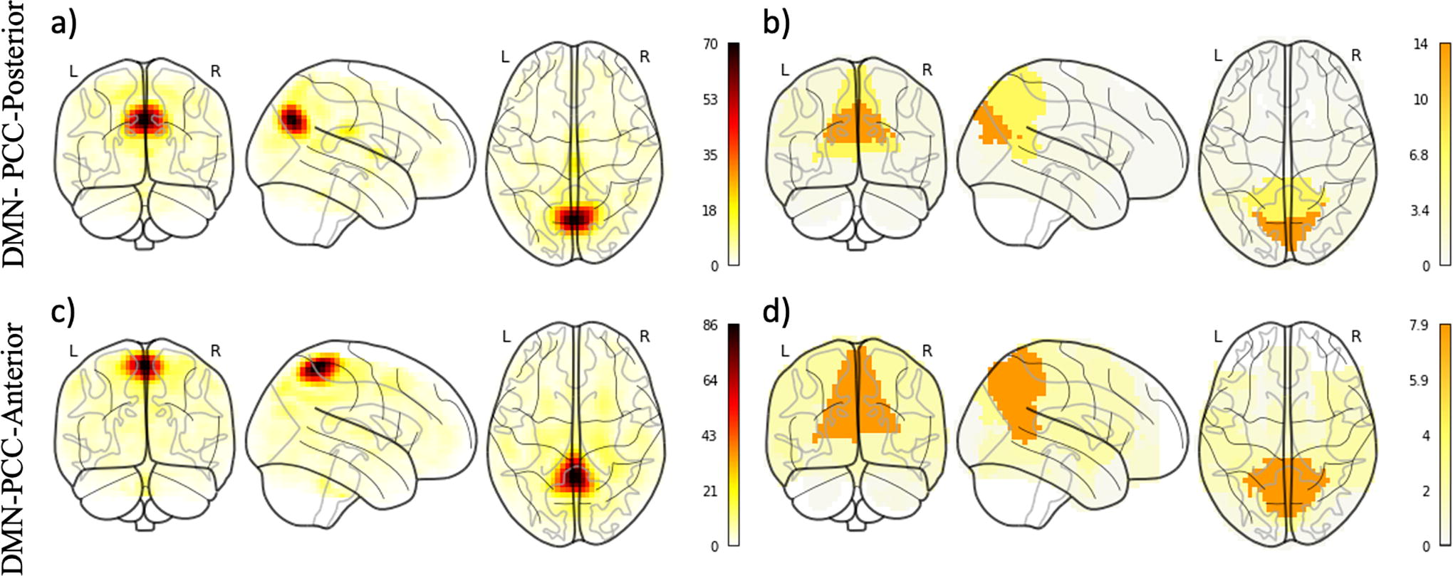
Glass brain representations of ICA components. On the left, sample group-averaged ICA components for the posterior (a) and anterior segments (c) of the DMN-PCC are shown. The right images demonstrate the atlas representations of misclassified ICA components: in (b), there is substantial involvement of the anterior posterior cingulate cortex (PCC) (yellow regions) that resulted in the misclassification of DMN-PCC-posterior as anterior and in (d), there is an equal representation of anterior and posterior DMN-PCC (orange regions), which resulted in misclassification of DMN-PCC-anterior as posterior. ICA, independent component analysis; DMN, Default Mode Network.

The most common misclassified functional regions are shown in Table 3. The total number of times these occur was relatively few compared with the total number of components and was therefore not considered a significant issue.

Table 3.

Top Five Misclassified Functional Regions—the Ground Truth and the Predicted Classification Along with the Number of Times the Pair Was Misclassified

Ground truth	Classification	Count
DMN-PCC-ANTERIOR	DMN-PCC-POSTERIOR	9
ATTENTION-DORSAL-IPS-MEDIAL	AUDITORY-LEFT	6
ATTENTION-DORSAL-IPS-MEDIAL	DMN-RSC	5
MOTOR_DORSAL_LEG	MOTOR_VENTRAL	5
MOTOR_DORSAL_LEG	DMN-CINGULATE-MID	5

Discussion

We introduced an accurate and efficient method for automated-labeling fMRI ICs based on their relationships to bilateral cortical brain areas using a publicly available standard atlas. We investigated the performance on healthy subjects in four different cohorts from the 1000 Functional Connectomes Project. The goal of this study was to provide an automated labeling technique that is based on the spatial relationship of the ICA signal and that goes beyond only distinguishing between noise ICs and non-noise ICs. Manually identifying RSNs can be a time-consuming and challenging task, especially when network components are fragmented into numerous subcomponents through IC analysis. The implementation of an automated process for labeling these network components and subcomponents could significantly streamline the process, saving time and improving result accuracy. Such automation can further promote the broader adoption of resting-state fMRI in various clinical applications.

Previous work

Prior spatial-based work attempted to relate IC and spatial information, although some studies did not use complete functional network coverage. One study by Vergun et al. (2016) focused on developing a method for extracting and classifying spatial maps into specific RSNs such as auditory, visual, default-mode, sensorimotor, and executive control networks. They compared various classifiers, including decision trees, perceptrons, naïve Bayes, and SVMs, achieving an accuracy of 88% for epilepsy patients using a naïve Bayes algorithm and 90% accuracy for healthy subjects using a perceptron. In comparison, this work only considered partial functional network coverage as they have only considered the abovementioned RSNs. Our work includes increased representation with the inclusion of language, salience, and attention to further improve the classification. De Martino et al. (De Martino et al., 2007) utilized an SVM classifier to classify ICs into six general classes based on an 11-feature fingerprint derived from IC’s voxel values distribution, spatial layout, as well as temporal and spectral properties. However, their study focused on task-based fMRI signals and only six classes of ICs. In contrast, our research expands the classification to 45 ICs, emphasizing the spatial localization and generalizable spatio-functional characteristics of ICs. In addition, our study benefits from a larger dataset of more than 100 subjects for both training and testing, enhancing reliability and generalizability. In the realm of deep learning approaches, groups have used deep 3D convolutional neural networks (Zhao et al., 2018), MLP Nozais et al. (2021), or Siamese network (Chou et al., 2022) for the classification of brain networks. Cumulatively, these approaches have a high accuracy; however, challenges such as manual labeling mistakes and inter-rater variability are inevitable when dealing with large training datasets. In our approach, atlas-based information benefits from the incorporation of local functionally coherent regions’ relative contribution to specific brain networks, in effect creating a brain-wide fingerprint for brain networks, Furthermore, atlas-based segmentations can further be incorporated into deep learning algorithms, although the improvement beyond utilizing a direct technique, as we currently proposed, is unclear.

Study limitations

This study created the framework to build an automated fMRI ICA component algorithm that is neither dependent on the anatomical atlas nor the labels for the ICA components. We showed that the framework is accurate with the Harvard-Oxford cortical and subcortical structural atlas and the labels herein. There are numerous other atlases available including some that are sparser and some that have finer definition of the brain regions. We believed that the Harvard-Oxford cortical and subcortical structural atlas provided the best balance between too few and too many anatomical regions, although others, for example, Talaraich, may provide higher accuracy.

There is a lack of universally accepted method for labeling of intrinsic brain networks. Although a universal taxonomy has been proposed (Uddin et al., 2019), it has not been widely utilized as of yet. Furthermore, the proposed taxonomy does not allow for the subsegmenation of larger networks into smaller subnetwork components (for example, specific labeling of the PCC cluster in the DMN). We therefore chose a scheme that is generally accepted currently in the literature and has been used at our institution for over a decade. Other ICA component naming should work as well; regardless of the naming convention, our results demonstrate the value of atlas-based classification of rs-fMRI, as the labels themselves may be modified according to user preference. There might also be a relationship with the number of ICA components (and labels) and the density of the atlas. We will explore this in future studies. This study also focused on the Beijing dataset as it was the largest (n = 198) and cleanest fMRI datasets in the 1000 Connectome data. The Cambridge_Buckner site has n = 198 datasets as well, but we found the Beijing data to be cleaner. In general, the framework laid out should work for any datasets, but it does a rigid registration to the atlas and therefore, if there are inconsistencies in the shape of the heads to the atlas template, then this could result in errors.

Our work focused on fMRI data from normal volunteers and therefore the alignment with the template T1 image in an atlas is not difficult. We did not test this approach with data of the patients who have deformations due to disease. This type of deformation would make the atlas alignment difficult depending on the degree of deformation. One method to work around would be to use a deformable registration algorithm to align the atlas T1 with the patient’s T1. The assumption is that the alignment of the sulci and gyri is possible, and this is another study we plan to complete.

Conclusions

We have successfully shown the feasibility of utilizing atlas-based labeling for rs-fMRI network ICA components, achieving high accuracy across various networks. This approach offers an interpretable method for labeling rs-fMRI ICAs. Future research avenues include investigating additional atlases and expanding the cohort to larger datasets. The implementation of an automated labeling process for network components has the potential to significantly reduce time requirements and improve result accuracy, thereby facilitating the wider adoption of rs-fMRI in diverse clinical applications.

Footnotes

Acknowledgments

We would like to thank the research groups that open-sourced their fMRI data as part of the 1000 Connectome Project.

Authors’ Contributions

H.K.: Methodology, Software, Data Curation, Writing—Original Draft, and Visualization; A.S.-P.: Methodology and Writing—Reviewing and Editing; I.T.: Methodology and Writing—Reviewing and Editing; L.L.: Methodology and Writing—Reviewing and Editing; E.B.: Methodology and Writing—Reviewing and Editing; H.S.: Conceptualization, Validation, Writing—Reviewing and Editing, Supervision, and Project Administration; C.J.: Conceptualization, Methodology, Validation, Writing—Reviewing and Editing, Supervision, and Project Administration.

Author Disclosure Statement

No competing financial interests exist.

Funding Information

No funding was received for this article.

Supplementary Material

Supplementary Table S1

References

Abou Elseoud

, Littow

, Remes

, et al. Group-ICA model order highlights patterns of functional brain connectivity. Front Syst Neurosci, 2011; 5:37; doi: 10.3389/fnsys.2011.00037

Beckmann

. Modelling with independent components. Neuroimage, 2012; 62(2):891–901; doi: 10.1016/j.neuroimage.2012.02.020

Bhaganagarapu

, Jackson

, Abbott

. An automated method for identifying artifact in independent component analysis of resting-state FMRI. Front Hum Neurosci, 2013; 7:343; doi: 10.3389/fnhum.2013.00343

Biswal

, Mennes

, Zuo

X-N

, et al. Toward discovery science of human brain function. Proc Natl Acad Sci U S A, 2010; 107(10):4734–4739; doi: 10.1073/pnas.0911855107

Calhoun

, Adali

. Unmixing FMRI with independent component analysis. IEEE Eng Med Biol Mag, 2006; 25(2):79–90; doi: 10.1109/memb.2006.1607672

Chou

, Chang

, Remedios

, et al. Automated classification of resting-state FMRI ICA components using a deep Siamese network. Front Neurosci, 2022; 16:768634; doi: 10.3389/fnins.2022.768634

De Martino

, Gentile

, Esposito

, et al. Classification of FMRI independent components using IC-fingerprints and support vector machine classifiers. Neuroimage, 2007; 34(1):177–194; doi: 10.1016/j.neuroimage.2006.08.041

Desikan

, Ségonne

, Fischl

, et al. An automated labeling system for subdividing the human cerebral cortex on MRI scans into gyral based regions of interest. Neuroimage, 2006; 31(3):968–980; doi: 10.1016/j.neuroimage.2006.01.021

Doucet

, Naveau

, Petit

, et al. Brain activity at rest: A multiscale hierarchical functional organization. J Neurophysiol, 2011; 105(6):2753–2763; doi: 10.1152/jn.00895.2010

10.

, Fan

. Group information guided ICA for FMRI data analysis. Neuroimage, 2013; 69:157–197; doi: 10.1016/j.neuroimage.2012.11.008

11.

Jenkinson

, Beckmann

, Behrens

TEJ

, et al. FSL. Neuroimage, 2012; 62(2):782–790; doi: 10.1016/j.neuroimage.2011.09.015

12.

, Jiang

, Li

, et al. Sparse representation of whole-brain FMRI signals for identification of functional networks. Med Image Anal, 2015; 20(1):112–134; doi: 10.1016/j.media.2014.10.011

13.

Mazoyer

, Mellet

, Perchey

, et al. BIL&GIN: A neuroimaging, cognitive, behavioral, and genetic database for the study of human brain lateralization. Neuroimage, 2016; 124(Pt B):1225–1231; doi: 10.1016/j.neuroimage.2015.02.071

14.

Mazziotta

, Toga

, Evans

, et al. A probabilistic atlas and reference system for the human brain: International Consortium for Brain Mapping (ICBM). Philos Trans R Soc Lond B Biol Sci, 2001; 356(1412):1293–1322; doi: 10.1098/rstb.2001.0915

15.

Nozais

, Boutinaud

, Verrecchia

, et al. Deep learning-based classification of resting-state FMRI independent-component analysis. Neuroinformatics, 2021; 19(4):619–637; doi: 10.1007/s12021-021-09514-x

16.

Smith

, Vidaurre

, Beckmann

, et al. Functional connectomics from resting-state FMRI. Trends Cogn Sci, 2013; 17(12):666–682; doi: 10.1016/j.tics.2013.09.016

17.

Tassi

, Maggioni

, Cerutti

, et al. A Novel Spatiotemporal Tool for the Automatic Classification of FMRI Noise Based on Independent Component Analysis. In: 2020 42nd Annual International Conference of the IEEE Engineering in Medicine & Biology Society (EMBC). 2020; pp. 1718–1721; doi: 10.1109/EMBC44109.2020.9176117

18.

Tohka

, Foerde

, Aron

, et al. Automatic independent component labeling for artifact removal in FMRI. Neuroimage, 2008; 39(3):1227–1245; doi: 10.1016/j.neuroimage.2007.10.013

19.

Uddin

, Yeo

BTT

, Spreng

. Towards a universal taxonomy of macro-scale functional human brain networks. Brain Topogr, 2019; 32(6):926–942; doi: 10.1007/s10548-019-00744-6

20.

Vergun

, Gaggl

, Nair

, et al. Classification and extraction of resting state networks using healthy and epilepsy FMRI data. Front Neurosci, 2016; 10:440; doi: 10.3389/fnins.2016.00440

21.

Zhao

, Dong

, Zhang

, et al. Automatic recognition of FMRI-derived functional networks using 3-D convolutional neural networks. IEEE Trans Biomed Eng, 2018; 65(9):1975–1984; doi: 10.1109/TBME.2017.2715281

Supplementary Material

Please find the following supplemental material available below.

For Open Access articles published under a Creative Commons License, all supplemental material carries the same license as the article it is associated with.

For non-Open Access articles published, all supplemental material carries a non-exclusive license, and permission requests for re-use of supplemental material or any part of supplemental material shall be sent directly to the copyright owner as specified in the copyright notice associated with the article.

0.00 MB

0.06 MB