Patient-Specific Whole-Body Attenuation Correction Maps from a CT System for Conjugate-View-Based Activity Quantification: Method Development and Evaluation
Available accessResearch articleFirst published online December, 2012
Patient-Specific Whole-Body Attenuation Correction Maps from a CT System for Conjugate-View-Based Activity Quantification: Method Development and Evaluation
For activity quantification based on planar scintillation camera measurements, photon attenuation is an important factor that needs to be corrected for in a patient- and organ-specific manner. One possibility for obtaining attenuation correction maps is to use X-ray CT scout images. Since the intensity of scout images is in relative numbers, their image values need to be multiplied by a factor to become quantitative and thus useful for attenuation correction. The calibration factor can for our current imaging system be obtained from a scanner system file, but is generally not available. For this purpose, a method based on the patient weight has been developed. Results based on 79 patient scout images show that the calibration factor thus determined correlates well with values that, in this case, are independently specified by the system. The accuracy of attenuation correction factors (ACFs) derived from the scout-based attenuation correction maps is evaluated by comparison to ACFs derived from three-dimensional CT studies. For photon energies of 208, 245, and 364 keV, scout-based ACFs are on average 1.2% and 0.5% from the CT-derived values, using the system-based and the weight-based values of the scout-image calibration factor, respectively. The imprecision is somewhat higher for the weight-based method, due to variability in the delineation of the patient contour used as a part of this method. In conclusion, X-ray scouts are found useful for attenuation correction with a satisfactory accuracy obtained, both using the new, weight-based method, and using the previous, system-based method, for determining the required calibration factor.
Introduction
In radionuclide therapy, the absorbed dose to different organs should be determined on an individual basis, especially in therapies where the absorbed dose approaches organ tolerance limits. Assessment of the absorbed dose requires that the cumulated activity in different organs is accurately quantified. The most widely used method for activity quantification remains planar scintillation camera imaging and the conjugate view method.1–4 In this method, a geometric mean is calculated of the count rate measured in two opposed scintillation camera images. This allows for the attenuation of the emitted photons to be described as a function of the total patient thickness along a direction parallel to the projection direction, at the location of the active region.1–3 Because of a considerable variation in body morphometry among patients and heterogeneous body composition, the attenuation needs to be estimated for each patient and each organ to be quantified. The attenuation distribution can be measured by use of two transmission studies, with and without the patient in position, where the ratio between these two images describes the fraction of photons transmitted through the patient. A common method for whole-body transmission measurements is by utilizing an external radionuclide source in the form of a 57Co flood source, mounted opposite to the scintillation camera head. However, due to limited activity in flood sources, the acquisition time is typically ∼20 minutes for a whole-body transmission scan, and images suffer from a relatively poor signal-to-noise ratio (SNR). Also, the transmission scan needs to be performed before administration of the radiopharmaceutical, since otherwise scattered photons emitted from the therapy radionuclide will contaminate the measured transmission count rate. Furthermore, when using a broad-beam source, such as an uncollimated flood source, combined with a large field-of-view scintillation camera, a non-negligible amount of unwanted scatter from the transmission radionuclide will be detected that will bias the measured attenuation values. Consequently, this scatter component needs to be accounted for in the subsequent scaling of the measured photon attenuation from the energy used for transmission scanning to the energy of the therapy radionuclide.5,6
An alternative method, proposed by our group, is to use an X-ray CT scout image for assessing the attenuation distribution.7 Due to the higher photon flux of the X-ray tube, it has a comparably high SNR and only takes about 2 minutes to acquire. Moreover, due to the fan-beam photon-emission geometry of the X-ray tube combined with collimated detectors, the amount of detected scatter is relatively low, which simplifies the necessary energy scaling between transmission and emission energies. Due to the high photon flux compared to the scatter from the therapy radionuclide, the scout image can also be acquired postinjection, which increases patient comfort and scanner throughput. An additional advantage is that the scout image provides excellent spatial resolution that is helpful for the definition of ROIs, for example, of the lung border.
Generally, the X-ray scout images from CT imaging systems are provided to delineate the longitudinal scan length of a CT study or for visual purposes, and are not quantitative. To be applicable for attenuation correction, the image values in the scout must be rescaled from the relative image values into absolute transmission values. This calibration factor is specific for every acquisition, and is in our previously published method7 obtained from a camera system file. For some camera systems, the calibration factor may be difficult, or even impossible, to retrieve, and we believe that this puts a limitation on a broader use of scout image-based attenuation correction maps. To make the scout-based method a more widespread option, an alternative, patient weight-based method is presented for determining attenuation maps calibrated in quantitative terms. To establish both this new method and the previously presented method, patient studies were evaluated by comparing scout image-based attenuation correction values in ROIs to those determined from three-dimensional (3D) CT studies. This is performed for photon energies of 70, 208, 245, and 364 keV, corresponding to the representative energy of the X-ray spectrum, and emission energies of 177Lu, 111In, and 131I, respectively.
Materials and Methods
Image data
Patient images are obtained from three different clinical radionuclide therapy studies involving patients on 177Lu-DOTA-octreotate with disseminated neuroendocrine tumors8 and 111In-labeled rituximab9 and 111In-labeled Zevalin™ in patients with non-Hodgkins B-cell lymphoma.10 Whole-body X-ray scout images for 31 different patients are included in the evaluation, where some of the patients have been imaged and weighed at several occasions with intervals of between 1 week and 2 months, so that altogether 79 scout images were obtained. For 10 of the patients, both scout images and CT studies have been acquired at the same imaging occasion, and for some patients, this procedure has been repeated up to four times. Included patients are 14 males and 17 females, where males have an average weight of 77 kg (range 62–93 kg) and a body–mass index (BMI) of 23.6 kg/m2 (range 18.9–26.0 kg/m2), whereas females have an average weight of 66.2 kg (range 44–90 kg) and a BMI of 20.7 kg/m2 (range 15.9–30.0 kg/m2). The patients included are thus a representative population, with a broad range of body morphometries.
Images are acquired using a Discovery VH SPECT/CT system (General Electric, Milwaukee, WI), including two scintillation camera heads and a single-slice CT unit (HawkEye™). Whole-body scintillation camera images are acquired in a 256×1024 matrix size with a pixel size of 2.21×2.21 mm2. Scout acquisitions are performed using a tube voltage of 140 kV, a tube current of 2.5 mA, and 0.5-mm Copper filtering, with a scanning time of ∼2 minutes for a whole-body scan. The acquired matrix has a size of 256×2000 pixels, and a pixel dimension in the vertical direction of 1.0 mm. In the lateral direction, the fan-beam acquisition geometry produces zooming by a factor that depends on the object distance from the X-ray tube, so that the pixel dimensions in the acquired matrix are not equal. In a previous work,7 the lateral pixel dimension was experimentally determined for a distance that corresponds to the central depth of the patient, and was obtained to 1.163 mm. To obtain the same image dimensions as for the whole-body scintillation camera images, the scout image is linearly interpolated into an image matrix with a size of 202×904, giving pixel dimensions of 2.21×2.21 mm2. The resulting image matrix is then padded with zeros, so that the final matrix dimensions become 256×1024. CT images are acquired using the same tube voltage and intensity as for the scout acquisition, with a rotation speed of 2.6 rpm. The time required is ∼10 minutes, yielding transaxial section images with an initial thickness of 1.0 cm, which are then down-sampled by the SPECT/CT system to different image dimensions, depending on the specifications given for the clinical SPECT studies that are acquired in parallel. The dimensions of the CT images are thus different for the different clinical studies from which data are obtained, and are either in a matrix size of 256×256×128 with voxel dimensions of 2.0×2.0×4.0 mm3, or in a 128×128×64 matrix with voxel dimensions of either 3.3×3.3×6.6 mm3 or 4.0×4.0×8.0 mm3. All image processing is performed offline by image export using the DICOM format and processing within LundADose software developed in IDL.11
In the further text and equations, bold symbols denote matrices. Image coordinates are denoted i, j, and l, where i runs along the patient's left–right direction; j runs along the head–foot direction; and l runs along the anterior–posterior direction. In equations where i, j, and l are not explicitly specified, all image coordinates are supposed to be included in the calculations.
Attenuation correction in the conjugate view method
The basic formalism underlying the conjugate view method can be found elsewhere.1–3 We have previously presented a pixel-based variant of this method that has been applied for quantification from whole-body scintillation camera images.8,12–14 Here, an activity image, A (MBq) is estimated using the expression:\documentclass{aastex}\usepackage{amsbsy}\usepackage{amsfonts}\usepackage{amssymb}\usepackage{bm}\usepackage{mathrsfs}\usepackage{pifont}\usepackage{stmaryrd}\usepackage{textcomp}\usepackage{portland, xspace}\usepackage{amsmath, amsxtra}\pagestyle{empty}\DeclareMathSizes{10}{9}{7}{6}\begin{document}\begin{align*}\textbf{\textit{A}} ( i , j ) = \varepsilon^{- 1} \cdot \textbf{\textit{AC}}_{Em} ( i , j ) \cdot \left[ Sc \left( \textbf{\textit{C}}_{Em}^{ant} ( i , j ) \right) \cdot Sc \left( \textbf{\textit{C}}_{Em}^{post} ( i , j ) \right) \right] ^{1 / 2} \tag{1}\end{align*}\end{document}
where ɛ is the scintillation camera system sensitivity (cpsMBq−1) measured in air, and \documentclass{aastex}\usepackage{amsbsy}\usepackage{amsfonts}\usepackage{amssymb}\usepackage{bm}\usepackage{mathrsfs}\usepackage{pifont}\usepackage{stmaryrd}\usepackage{textcomp}\usepackage{portland, xspace}\usepackage{amsmath, amsxtra}\pagestyle{empty}\DeclareMathSizes{10}{9}{7}{6}\begin{document}$$\textbf{\textit{C}}_{Em}^{ant}$$\end{document} and \documentclass{aastex}\usepackage{amsbsy}\usepackage{amsfonts}\usepackage{amssymb}\usepackage{bm}\usepackage{mathrsfs}\usepackage{pifont}\usepackage{stmaryrd}\usepackage{textcomp}\usepackage{portland, xspace}\usepackage{amsmath, amsxtra}\pagestyle{empty}\DeclareMathSizes{10}{9}{7}{6}\begin{document}$$\textbf{\textit{C}}_{Em}^{post}$$\end{document} (cps) are anterior- and posterior-view count-rate images acquired for the photon energy, Em, of the imaging radionuclide. The function Sc denotes scatter correction of the count-rate images, which in our implementation is performed using deconvolution by scatter-point spread functions determined from Monte Carlo simulation.15 The image ACEm is the attenuation correction map valid for Em, as described in detail below. Before application of Equation 1, the image ACEm is convolved with a Gaussian function with a similar spatial resolution as that of the emission images. Furthermore, the images \documentclass{aastex}\usepackage{amsbsy}\usepackage{amsfonts}\usepackage{amssymb}\usepackage{bm}\usepackage{mathrsfs}\usepackage{pifont}\usepackage{stmaryrd}\usepackage{textcomp}\usepackage{portland, xspace}\usepackage{amsmath, amsxtra}\pagestyle{empty}\DeclareMathSizes{10}{9}{7}{6}\begin{document}$$\textbf{\textit{C}}_{Em}^{ant}$$\end{document} and \documentclass{aastex}\usepackage{amsbsy}\usepackage{amsfonts}\usepackage{amssymb}\usepackage{bm}\usepackage{mathrsfs}\usepackage{pifont}\usepackage{stmaryrd}\usepackage{textcomp}\usepackage{portland, xspace}\usepackage{amsmath, amsxtra}\pagestyle{empty}\DeclareMathSizes{10}{9}{7}{6}\begin{document}$$\textbf{\textit{C}}_{Em}^{post}$$\end{document}are spatially registered to ACEm (Fig. 1E) by a method tailored for whole-body images.16 For activity quantification of organs, the activity image, A, is further processed by drawing ROIs, correcting for background and overlapping activities, and application of a source thickness correction calculated for each ROI.12 A perhaps more common way of implementing the conjugate view method is to delineate organ ROIs directly on the anterior–posterior count-rate images, and then perform the geometric mean calculation on the total count rate determined from each ROI.3 Attenuation correction is then performed by multiplying this geometric mean value by an attenuation correction factor (ACFEm). The ACFEm is typically determined by delineating organ ROIs in the attenuation correction map and determining the ROI mean value, that is, \documentclass{aastex}\usepackage{amsbsy}\usepackage{amsfonts}\usepackage{amssymb}\usepackage{bm}\usepackage{mathrsfs}\usepackage{pifont}\usepackage{stmaryrd}\usepackage{textcomp}\usepackage{portland, xspace}\usepackage{amsmath, amsxtra}\pagestyle{empty}\DeclareMathSizes{10}{9}{7}{6}\begin{document}$${\rm ACF}_{Em} = \overline{\textbf{\textit{AC}}_{Em}} ( i , j \in ROI )$$\end{document}. In either of the implementation schemes, region- as well as pixel-based, an attenuation correction map is required.
(A–C) Scout-based attenuation correction map of one male patient, with (A) the patient contour used for calculation of the weight-based calibration factor, (B) the border of the regions used for the different fractions of bony and soft tissue in the weighting image W, (C) the ROIs used for evaluation of the ACF in different organs. Image (D) shows the CT-based attenuation correction map that is spatially registered to the scout, with organ ROIs; (E) shows the activity image A (Equation 1) overlaid on the scout attenuation correction map, and (F) shows the activity image with organ ROIs typically used for activity quantification. ACF, attenuation correction factor. Color images available online at www.liebertpub.com/cbr
A general model expression of an attenuation correction map valid for an arbitrary photon energy E can be described according to the following equation:\documentclass{aastex}\usepackage{amsbsy}\usepackage{amsfonts}\usepackage{amssymb}\usepackage{bm}\usepackage{mathrsfs}\usepackage{pifont}\usepackage{stmaryrd}\usepackage{textcomp}\usepackage{portland, xspace}\usepackage{amsmath, amsxtra}\pagestyle{empty}\DeclareMathSizes{10}{9}{7}{6}\begin{document}\begin{align*}\textbf{\textit{AC}}_E ( i , j ) = \left[ exp ( \textbf{\textit{R}}_E ( i , j ) ) \right] ^{1 / 2} \tag{2}\end{align*}\end{document}
with\documentclass{aastex}\usepackage{amsbsy}\usepackage{amsfonts}\usepackage{amssymb}\usepackage{bm}\usepackage{mathrsfs}\usepackage{pifont}\usepackage{stmaryrd}\usepackage{textcomp}\usepackage{portland, xspace}\usepackage{amsmath, amsxtra}\pagestyle{empty}\DeclareMathSizes{10}{9}{7}{6}\begin{document}\begin{align*}\textbf{\textit{R}}_E ( i , j ) = \int \limits_0^{\textbf{\textit{L}} ( i , j )} {\bold \mu}_E ( i , j , l ) {\rm d}l = \int \limits_0^{\textbf{\textit{L}} (i , j)} ({\bold \mu} / {\bold \rho} ) _E ( i , j , l ) \cdot {\bold \rho} ( i , j , l) {\rm d}l \tag{3}\end{align*}\end{document}
In this equation, l is the continuous coordinate along the anterior–posterior projection line, and L(i, j) is the physical patient thickness (cm) at each image position (i, j). The 3D distributions μE and (μ/ρ)E describe the linear attenuation coefficient (cm−1), and the mass attenuation coefficient (cm2g−1), respectively, at different positions in the patient for the photon energy E. The 3D distribution ρ is the mass density (g cm3) and RE is a unitless 2D matrix describing the line integral of the various attenuation coefficients that the photons encounter along their passage through the patient.
The attenuation correction maps, or ACFs, are commonly measured using transmission imaging with and without the patient in position.3 For the X-ray scout, a single value representative of the count rate in air, that is, without the patient in position, is obtained from the mandatory CT calibration procedure. The acquired scout image obtained from the X-ray system is a version of the image RE in Equation 3, with E equal to the transmission photon energy, Et, that is, REt. For the scout image, Et is really the photon energy spectrum of the X-ray system, which, for our system, was previously found to be well represented by an energy of 70 keV.7 However, the scout image is in relative values that need to be rescaled to obtain the quantitative image REt. Denoting the raw acquired scout image by S0, the values in S0 range between the camera-specific values smin and smax (for our system equal to −1000 and 3096, respectively). Following our previous work,7 an estimate of the image REt, that is, \documentclass{aastex}\usepackage{amsbsy}\usepackage{amsfonts}\usepackage{amssymb}\usepackage{bm}\usepackage{mathrsfs}\usepackage{pifont}\usepackage{stmaryrd}\usepackage{textcomp}\usepackage{portland, xspace}\usepackage{amsmath, amsxtra}\pagestyle{empty}\DeclareMathSizes{10}{9}{7}{6}\begin{document}$$\hat {\textbf{\textit{R}}}_{Et}$$\end{document} is determined from S0 by renormalization to the image S and then scaling by an acquisition-specific calibration factor, c (unitless), according to the following equation:\documentclass{aastex}\usepackage{amsbsy}\usepackage{amsfonts}\usepackage{amssymb}\usepackage{bm}\usepackage{mathrsfs}\usepackage{pifont}\usepackage{stmaryrd}\usepackage{textcomp}\usepackage{portland, xspace}\usepackage{amsmath, amsxtra}\pagestyle{empty}\DeclareMathSizes{10}{9}{7}{6}\begin{document}\begin{align*}\hat {\textbf{\textit{R}}}_{Et} ( i , j ) = c \cdot( \textbf{\textit{S}}_0 ( i , j ) - s_{min} ) / ( s_{max} - s_{min} )= c \cdot \textbf{\textit{S}} ( {i , j} ) \tag{4}\end{align*}\end{document}
where the minimum value in S is thus zero, and (smax–smin) equals 4096 for our system. The factor c thus constitutes the link between the relative image S and the quantitative image. \documentclass{aastex}\usepackage{amsbsy}\usepackage{amsfonts}\usepackage{amssymb}\usepackage{bm}\usepackage{mathrsfs}\usepackage{pifont}\usepackage{stmaryrd}\usepackage{textcomp}\usepackage{portland, xspace}\usepackage{amsmath, amsxtra}\pagestyle{empty}\DeclareMathSizes{10}{9}{7}{6}\begin{document}$$\hat {\textbf{\textit{R}}}_{Et}$$\end{document}. In our previous work, the factor c was obtained from a system file in the SPECT/CT scanner.7 For situations when this factor is not available from the system, an alternative method of obtaining the factor c is derived.
Determination of the weight-based calibration factor
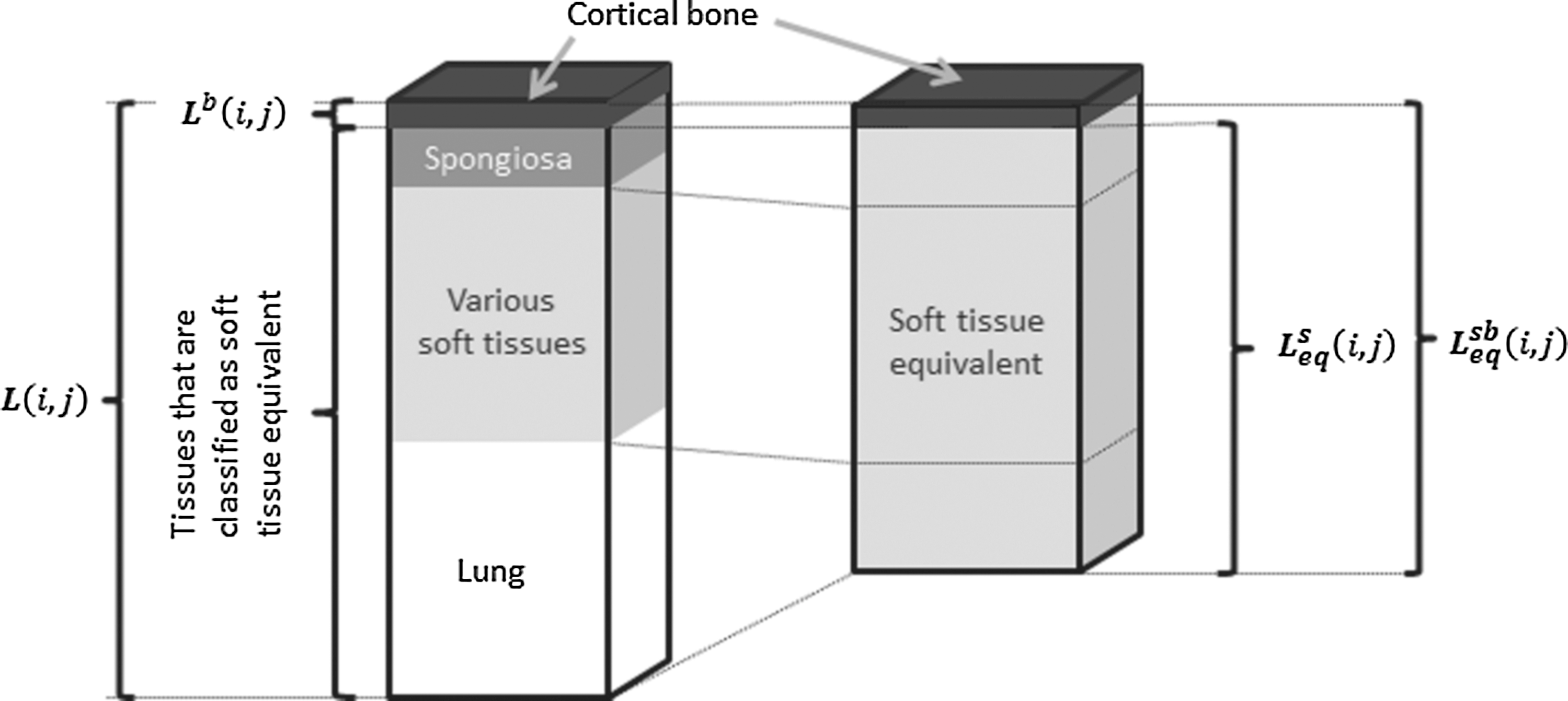
As seen from Equation 3, the physical factors that govern the distribution RE (or REt) are the distributions of the mass attenuation coefficient and the mass density. The difference between the mass attenuation coefficients of various soft tissues is small, since the dominant photon interaction process is by Compton scattering. For instance, for 70 keV photons, the mass attenuation coefficient equals 0.194 g cm2 for both lung and soft tissue,17,18 and the difference in the linear attenuation coefficient is governed by the difference in mass densities. For bony tissues, the linear attenuation coefficient is increased due to a higher probability for photoelectric absorption. However, there is a marked difference between spongiosa and cortical bone, and for energies above 70 keV, the value of the linear attenuation coefficient of spongiosa is closer to that of soft tissue than of cortical bone.17–19 Although the amount of cortical bone is in many regions small,20 it affects the image REt due to the relatively high value of the linear attenuation coefficient. However, the amount of cortical bone along the projection line is not available from the planar scout image, and to arrive at a quantitative estimate of REt, approximations are required, as derived in Appendix 1. Following these derivations, with approximations illustrated in Figure 2, the expression for the weight-based calibration factor, cW, is obtained as follows:\documentclass{aastex}\usepackage{amsbsy}\usepackage{amsfonts}\usepackage{amssymb}\usepackage{bm}\usepackage{mathrsfs}\usepackage{pifont}\usepackage{stmaryrd}\usepackage{textcomp}\usepackage{portland, xspace}\usepackage{amsmath, amsxtra}\pagestyle{empty}\DeclareMathSizes{10}{9}{7}{6}\begin{document}\begin{align*} \begin{split}c_W & = \hat{m}_{TB} ( \Delta i \Delta j ) ^{- 1} \left\{ \mathop\sum_{i , j \in pat} \textbf{\textit{S}} ( i , j ) \cdot [ \rho^s \textbf{\textit{W}} ( i , j ) + \rho^b ( 1 - \textbf{\textit{W}} (i , j))] \cdot [ \mu_{Et}^s \textbf{\textit{W}} (i , j) + \mu_{Et}^b ( 1 - \textbf{\textit{W}}(i , j))] ^{-1} \right\}^{-1}\end{split} \tag{{\rm A}8} \end{align*}\end{document}
Illustration of the approximations made in the derived equations. The physical thickness of the patient at a location corresponding to the pixel coordinates (i,j) is denoted L(i,j). It is constituted of different amounts of cortical bone, spongiosa, various soft tissues, and lung. The thickness seen by the x-rays is a “radiological thickness” denoted RE (Equation 3). The underlying idea is that RE can be represented by a sum of two compartments, a soft tissue-equivalent compartment and a compartment of cortical bone, where the respective contributions are given by the product of the linear attenuation coefficient and the equivalent thicknesses (Equation A5). The soft tissue- and bone-equivalent thickness \documentclass{aastex}\usepackage{amsbsy}\usepackage{amsfonts}\usepackage{amssymb}\usepackage{bm}\usepackage{mathrsfs}\usepackage{pifont}\usepackage{stmaryrd}\usepackage{textcomp}\usepackage{portland, xspace}\usepackage{amsmath, amsxtra}\pagestyle{empty}\DeclareMathSizes{10}{9}{7}{6}\begin{document}$$L^{sb}_{eq}$$\end{document} is the sum of the equivalent thickness of cortical bone, (1−W)\documentclass{aastex}\usepackage{amsbsy}\usepackage{amsfonts}\usepackage{amssymb}\usepackage{bm}\usepackage{mathrsfs}\usepackage{pifont}\usepackage{stmaryrd}\usepackage{textcomp}\usepackage{portland, xspace}\usepackage{amsmath, amsxtra}\pagestyle{empty}\DeclareMathSizes{10}{9}{7}{6}\begin{document}$$L^{sb}_{eq}$$\end{document}, and the soft tissue-equivalent thickness, \documentclass{aastex}\usepackage{amsbsy}\usepackage{amsfonts}\usepackage{amssymb}\usepackage{bm}\usepackage{mathrsfs}\usepackage{pifont}\usepackage{stmaryrd}\usepackage{textcomp}\usepackage{portland, xspace}\usepackage{amsmath, amsxtra}\pagestyle{empty}\DeclareMathSizes{10}{9}{7}{6}\begin{document}$$L^{s}_{eq} = WL^{sb}_{eq}$$\end{document} (Equations Al and A2). The equivalent thickness of cortical bone is assumed to be equal to the physical thickness, Lb, whereas the soft tissue-equivalent thickness \documentclass{aastex}\usepackage{amsbsy}\usepackage{amsfonts}\usepackage{amssymb}\usepackage{bm}\usepackage{mathrsfs}\usepackage{pifont}\usepackage{stmaryrd}\usepackage{textcomp}\usepackage{portland, xspace}\usepackage{amsmath, amsxtra}\pagestyle{empty}\DeclareMathSizes{10}{9}{7}{6}\begin{document}$$L^{s}_{eq}$$\end{document} represents contributions from spongiosa, soft tissues, and lung (Equation Al).
where \documentclass{aastex}\usepackage{amsbsy}\usepackage{amsfonts}\usepackage{amssymb}\usepackage{bm}\usepackage{mathrsfs}\usepackage{pifont}\usepackage{stmaryrd}\usepackage{textcomp}\usepackage{portland, xspace}\usepackage{amsmath, amsxtra}\pagestyle{empty}\DeclareMathSizes{10}{9}{7}{6}\begin{document}$$\hat{m}_{TB}$$\end{document} (g) is the patient weight as measured from a scale; ΔiΔj is the pixel area (cm2); ρsand ρb are the mass densities (g cm3) of soft tissue and cortical bone, respectively, and \documentclass{aastex}\usepackage{amsbsy}\usepackage{amsfonts}\usepackage{amssymb}\usepackage{bm}\usepackage{mathrsfs}\usepackage{pifont}\usepackage{stmaryrd}\usepackage{textcomp}\usepackage{portland, xspace}\usepackage{amsmath, amsxtra}\pagestyle{empty}\DeclareMathSizes{10}{9}{7}{6}\begin{document}$$\mu_{Et}^s$$\end{document} and \documentclass{aastex}\usepackage{amsbsy}\usepackage{amsfonts}\usepackage{amssymb}\usepackage{bm}\usepackage{mathrsfs}\usepackage{pifont}\usepackage{stmaryrd}\usepackage{textcomp}\usepackage{portland, xspace}\usepackage{amsmath, amsxtra}\pagestyle{empty}\DeclareMathSizes{10}{9}{7}{6}\begin{document}$$\mu_{Et}^b$$\end{document} (cm−1) are the linear attenuation coefficients for soft tissue and cortical bone for the transmission photon energy, respectively.17,18 The summation is performed over pixels with coordinates (i and j) that represent the patient in the image. The distribution W is a matrix of weighing factors with a maximum value of one, describing the position-dependent fraction of the soft tissue- and bone-equivalent thickness distribution \documentclass{aastex}\usepackage{amsbsy}\usepackage{amsfonts}\usepackage{amssymb}\usepackage{bm}\usepackage{mathrsfs}\usepackage{pifont}\usepackage{stmaryrd}\usepackage{textcomp}\usepackage{portland, xspace}\usepackage{amsmath, amsxtra}\pagestyle{empty}\DeclareMathSizes{10}{9}{7}{6}\begin{document}$$L_{eq}^{sb}$$\end{document} that is represented by soft tissue (see Appendix 1).
In Equation A8, the image S is determined from the measured scout image and Equation 4, and the pixel area is determined by standard camera calibration procedures. The pixel coordinates (i and j) belonging to the area occupied by the patient are determined by applying a segmentation procedure in the image S. The patient contour is delineated by applying the automatic threshold method by Otsu,21,22 so that the patient contour is precisely enclosed (Fig. 1A). For patients who have a metal hip implant, which results in a very high-intensity focus in the scout image, some more elaboration is required. Due to a higher probability for photoelectric interaction in metal, it is not well approximated by body tissue, so that Equation A8 gives a poorer approximation in such cases. Also, the high-intensity focus presents a problem for the automatic segmentation procedure, reducing its ability to estimate the threshold for the patient contour. In this work, two of the evaluated patients have a hip implant, and this has been practically handled by manually delineating a region over the hip implant in the image S and replacing the pixel values by values just beside the region. Smaller metal details such as bracelets or teeth are left unprocessed. The weighing factors in W are not available from the planar scout image, and to determine this distribution, some assumptions need to be made. In this work, the values in W are set for different regions that are manually marked on the image S, as displayed in Figure 1B. The weighing factors have been previously determined by comparison of the values in a projected whole-body CT with the corresponding scout image values for one male patient. The values in W were thus determined to 0.9, 1.0, and 0.9 for the head, the upper torso, and the pelvis–legs, respectively.14 For investigation of the sensitivity to the inclusion (or exclusion) of the partitioning distribution W in Equation A8, an expression where W(i,j) is set to unity everywhere is also given as \documentclass{aastex}\usepackage{amsbsy}\usepackage{amsfonts}\usepackage{amssymb}\usepackage{bm}\usepackage{mathrsfs}\usepackage{pifont}\usepackage{stmaryrd}\usepackage{textcomp}\usepackage{portland, xspace}\usepackage{amsmath, amsxtra}\pagestyle{empty}\DeclareMathSizes{10}{9}{7}{6}\begin{document}$$c{\prime}_W$$\end{document} according to Equation A9 (Appendix 1).
Application of the calibration factor to obtain the attenuation correction map
By use of Equations 4 and 2, a scout-based attenuation correction map valid for the transmission imaging energy, ACEt, may be obtained. In Equation 4, the factor c can thus either be the scanner system-based calibration factor, further denoted csys, or the weight-based calibration factor, cW. To obtain an attenuation correction map for the emission imaging energy, ACEm, to be applied in Equation 1, an energy scaling is required from Et to the energy of the imaging radionuclide, Em. This is performed by use of Equations 2, A5, and A6, so that\documentclass{aastex}\usepackage{amsbsy}\usepackage{amsfonts}\usepackage{amssymb}\usepackage{bm}\usepackage{mathrsfs}\usepackage{pifont}\usepackage{stmaryrd}\usepackage{textcomp}\usepackage{portland, xspace}\usepackage{amsmath, amsxtra}\pagestyle{empty}\DeclareMathSizes{10}{9}{7}{6}\begin{document}\begin{align*} \begin{split} & \textbf{\textit{AC}}_{Em} (i , j) = \left[exp (\hat {\textbf{\textit{R}}}_{Em} (i , j)) \right]^{1/2} \\& = \left(exp \left[\left( \frac {{\mu_{Em}^s} \textbf{\textit{W}}(i , j) + {\mu_{Em}^b} (1-\textbf{\textit{W}}(i , j))} {\mu_{Et}^s \textbf{\textit{W}} (i , j) + \mu_{Et}^b (1- \textbf{\textit{W}} (i , j))} \right) \cdot c_x \cdot{\textbf{\textit{S}} (i , j)} \right] \right)^{1/2}\end{split} \tag{5}\end{align*}\end{document}
where cx temporarily denotes either csys or cW. The factors \documentclass{aastex}\usepackage{amsbsy}\usepackage{amsfonts}\usepackage{amssymb}\usepackage{bm}\usepackage{mathrsfs}\usepackage{pifont}\usepackage{stmaryrd}\usepackage{textcomp}\usepackage{portland, xspace}\usepackage{amsmath, amsxtra}\pagestyle{empty}\DeclareMathSizes{10}{9}{7}{6}\begin{document}$$\mu_{Em}^s$$\end{document} and \documentclass{aastex}\usepackage{amsbsy}\usepackage{amsfonts}\usepackage{amssymb}\usepackage{bm}\usepackage{mathrsfs}\usepackage{pifont}\usepackage{stmaryrd}\usepackage{textcomp}\usepackage{portland, xspace}\usepackage{amsmath, amsxtra}\pagestyle{empty}\DeclareMathSizes{10}{9}{7}{6}\begin{document}$$\mu_{Em}^b$$\end{document} are the linear attenuation coefficients for soft tissue and bone, respectively, for the energy of the emission imaging radionuclide.18 It should be noted that since linear attenuation coefficients are applied in this equation, it is assumed that scatter correction is performed before attenuation correction, following Equation 1. When explicit scatter correction of count-rate images is not performed, a commonly used method is to apply an effective attenuation coefficient in the attenuation correction.3,5,6 The use of such a scheme can be incorporated in Equation 5 by substituting \documentclass{aastex}\usepackage{amsbsy}\usepackage{amsfonts}\usepackage{amssymb}\usepackage{bm}\usepackage{mathrsfs}\usepackage{pifont}\usepackage{stmaryrd}\usepackage{textcomp}\usepackage{portland, xspace}\usepackage{amsmath, amsxtra}\pagestyle{empty}\DeclareMathSizes{10}{9}{7}{6}\begin{document}$$\mu_{Em}^s$$\end{document} and \documentclass{aastex}\usepackage{amsbsy}\usepackage{amsfonts}\usepackage{amssymb}\usepackage{bm}\usepackage{mathrsfs}\usepackage{pifont}\usepackage{stmaryrd}\usepackage{textcomp}\usepackage{portland, xspace}\usepackage{amsmath, amsxtra}\pagestyle{empty}\DeclareMathSizes{10}{9}{7}{6}\begin{document}$$\mu_{Em}^b$$\end{document} for the effective attenuation coefficients, whose values must then be determined by separate measurements. The attenuation coefficients \documentclass{aastex}\usepackage{amsbsy}\usepackage{amsfonts}\usepackage{amssymb}\usepackage{bm}\usepackage{mathrsfs}\usepackage{pifont}\usepackage{stmaryrd}\usepackage{textcomp}\usepackage{portland, xspace}\usepackage{amsmath, amsxtra}\pagestyle{empty}\DeclareMathSizes{10}{9}{7}{6}\begin{document}$$\mu_{Et}^s$$\end{document} and \documentclass{aastex}\usepackage{amsbsy}\usepackage{amsfonts}\usepackage{amssymb}\usepackage{bm}\usepackage{mathrsfs}\usepackage{pifont}\usepackage{stmaryrd}\usepackage{textcomp}\usepackage{portland, xspace}\usepackage{amsmath, amsxtra}\pagestyle{empty}\DeclareMathSizes{10}{9}{7}{6}\begin{document}$$\mu_{Et}^b$$\end{document} in the denominator should in any method be the linear ones, since these are applied to convert the scout image, which is assumed to be acquired in a narrow-beam geometry, to a map of the soft-tissue equivalent thickness. At application of the attenuation correction in Equation 1, the values in the image ACEm for locations outside the patient should have a value of one, as seen from Equations 2 and 3 where zero attenuation gives RE(i, j)=0 and ACE(i, j)=1. After calculation of ACEm, the image values outside the patient contour are therefore explicitly set to one.
In Equations A8 and 5 the values used for the physical parameters, \documentclass{aastex}\usepackage{amsbsy}\usepackage{amsfonts}\usepackage{amssymb}\usepackage{bm}\usepackage{mathrsfs}\usepackage{pifont}\usepackage{stmaryrd}\usepackage{textcomp}\usepackage{portland, xspace}\usepackage{amsmath, amsxtra}\pagestyle{empty}\DeclareMathSizes{10}{9}{7}{6}\begin{document}$$\mu_{Et}^s , \mu_{Et}^b , \mu_{Em}^s , \mu_{Em}^b , \rho^s$$\end{document}and ρb are obtained from the National Institute of Standards and Technology (NIST).18 For soft tissue, reference values for ICRU Four Component Soft Tissue17 are used, giving for 70 keV photons \documentclass{aastex}\usepackage{amsbsy}\usepackage{amsfonts}\usepackage{amssymb}\usepackage{bm}\usepackage{mathrsfs}\usepackage{pifont}\usepackage{stmaryrd}\usepackage{textcomp}\usepackage{portland, xspace}\usepackage{amsmath, amsxtra}\pagestyle{empty}\DeclareMathSizes{10}{9}{7}{6}\begin{document}$$( \mu / \rho ) _{70}^s$$\end{document}=0.1934 g cm2 and ρs=1.0 g cm3. For cortical bone, values for Cortical Bone ICRU-4417 are used, giving for 70 keV \documentclass{aastex}\usepackage{amsbsy}\usepackage{amsfonts}\usepackage{amssymb}\usepackage{bm}\usepackage{mathrsfs}\usepackage{pifont}\usepackage{stmaryrd}\usepackage{textcomp}\usepackage{portland, xspace}\usepackage{amsmath, amsxtra}\pagestyle{empty}\DeclareMathSizes{10}{9}{7}{6}\begin{document}$$( \mu / \rho ) _{70}^b$$\end{document}=0.269 g cm2 and ρb=1.92 g cm3.
The practical steps required to implement the weight-based calibration method for obtaining a scout-based attenuation correction map are summarized in Appendix 2.
Evaluation
First, the underlying idea that the patient weight can be estimated from scout images was tested by application of Equation A7 to the 79 patient S images and using csys. For the same studies, the values of cW were then determined using Equation A8 and compared to the values of csys.
The accuracy of the scout image-based maps, ACEt and ACEm, was determined by a comparison to independently obtained AC maps from CT measurements, which, unlike the scout image values, were quantitative. From a CT image, an estimate of the 3D map of the linear attenuation coefficients, \documentclass{aastex}\usepackage{amsbsy}\usepackage{amsfonts}\usepackage{amssymb}\usepackage{bm}\usepackage{mathrsfs}\usepackage{pifont}\usepackage{stmaryrd}\usepackage{textcomp}\usepackage{portland, xspace}\usepackage{amsmath, amsxtra}\pagestyle{empty}\DeclareMathSizes{10}{9}{7}{6}\begin{document}$$\hat {\mu}_E$$\end{document}(cm−1) was determined as\documentclass{aastex}\usepackage{amsbsy}\usepackage{amsfonts}\usepackage{amssymb}\usepackage{bm}\usepackage{mathrsfs}\usepackage{pifont}\usepackage{stmaryrd}\usepackage{textcomp}\usepackage{portland, xspace}\usepackage{amsmath, amsxtra}\pagestyle{empty}\DeclareMathSizes{10}{9}{7}{6}\begin{document}\begin{align*}\hat {\mu}_E ( i , j , l ) = ( \mu / \rho ) _{E} \cdot \hat{\bold \rho} ( i , j , l ) \tag{6}\end{align*}\end{document}
where \documentclass{aastex}\usepackage{amsbsy}\usepackage{amsfonts}\usepackage{amssymb}\usepackage{bm}\usepackage{mathrsfs}\usepackage{pifont}\usepackage{stmaryrd}\usepackage{textcomp}\usepackage{portland, xspace}\usepackage{amsmath, amsxtra}\pagestyle{empty}\DeclareMathSizes{10}{9}{7}{6}\begin{document}$$\hat{\bold \rho}$$\end{document}(g cm3) is an estimate of the mass density distribution, ρ, of the patient. The distribution \documentclass{aastex}\usepackage{amsbsy}\usepackage{amsfonts}\usepackage{amssymb}\usepackage{bm}\usepackage{mathrsfs}\usepackage{pifont}\usepackage{stmaryrd}\usepackage{textcomp}\usepackage{portland, xspace}\usepackage{amsmath, amsxtra}\pagestyle{empty}\DeclareMathSizes{10}{9}{7}{6}\begin{document}$$\hat{\bold \rho}$$\end{document} was obtained using a bilinear function, φ following\documentclass{aastex}\usepackage{amsbsy}\usepackage{amsfonts}\usepackage{amssymb}\usepackage{bm}\usepackage{mathrsfs}\usepackage{pifont}\usepackage{stmaryrd}\usepackage{textcomp}\usepackage{portland, xspace}\usepackage{amsmath, amsxtra}\pagestyle{empty}\DeclareMathSizes{10}{9}{7}{6}\begin{document}\begin{align*}\hat {\rho} ( i , j , l ) = \phi ( I ( i , j , l )) = \begin{cases}a_1 + b_1 \cdot ( I ( i , j , l ) ) ; ( I ( i , j, l ) ) < H_1 \\ a_2 + b_2 \cdot ( I ( i , j , l ) ) ; ( I ( i , j, l ) ) \ge H_1\end{cases} \tag{7}\end{align*}\end{document}
where I(i, j, l) is the CT image values (Hounsfield units, HU), added by a value of 1000. The values of the parameters in this equation were determined by measurement of a standard calibration phantom,23 by determining the HU of eight tissue-equivalent inserts with various mass densities and fitting a bilinear function to the density-versus-HU data, as previously described in.12,24 The parameter values were a1=−1.57×10⁻² (g/cm3), b1=1.03×10⁻³ (g/cm3/HU), a2=2.94×10⁻¹ (g/cm3), b2=7.31×10⁻⁴ (g/cm3/HU), and H1=1025 (HU). The mass attenuation coefficients \documentclass{aastex}\usepackage{amsbsy}\usepackage{amsfonts}\usepackage{amssymb}\usepackage{bm}\usepackage{mathrsfs}\usepackage{pifont}\usepackage{stmaryrd}\usepackage{textcomp}\usepackage{portland, xspace}\usepackage{amsmath, amsxtra}\pagestyle{empty}\DeclareMathSizes{10}{9}{7}{6}\begin{document}$$( \mu / \rho ) _{E}$$\end{document} for soft tissue, skeleton spongiosa, and cortical bone were obtained from NIST18 and ICRU Report 4619 for the energies of interest, E=Et (70 keV) and E=Em (208, 245, and 364 keV). A classification of the voxels in the mass density image was performed, where values <1.051 g cm3 were classified as soft tissue, values above 1.2 g cm3 as cortical bone, and intermediate values as spongiosa. The respective mass attenuation coefficient was then multiplied by the mass density value for the respective set of voxels. It should be noted that although a voxel classification was made for selecting the mass attenuation coefficient value, the mass densities as well as the linear attenuation coefficients were determined on a voxel-by-voxel basis. A CT-based image \documentclass{aastex}\usepackage{amsbsy}\usepackage{amsfonts}\usepackage{amssymb}\usepackage{bm}\usepackage{mathrsfs}\usepackage{pifont}\usepackage{stmaryrd}\usepackage{textcomp}\usepackage{portland, xspace}\usepackage{amsmath, amsxtra}\pagestyle{empty}\DeclareMathSizes{10}{9}{7}{6}\begin{document}$$R_E^{CT}$$\end{document}was then calculated by numerical integration along the anterior–posterior direction:\documentclass{aastex}\usepackage{amsbsy}\usepackage{amsfonts}\usepackage{amssymb}\usepackage{bm}\usepackage{mathrsfs}\usepackage{pifont}\usepackage{stmaryrd}\usepackage{textcomp}\usepackage{portland, xspace}\usepackage{amsmath, amsxtra}\pagestyle{empty}\DeclareMathSizes{10}{9}{7}{6}\begin{document}\begin{align*} \textbf{\textit{R}}_E^{CT} (i , j) = \Delta l \cdot{\mathop\sum_l} \hat{\mu}_E (i , j , l) \tag{8} \end{align*}\end{document}
where Δl is the voxel dimension in the anterior–posterior direction (cm). An attenuation correction map, \documentclass{aastex}\usepackage{amsbsy}\usepackage{amsfonts}\usepackage{amssymb}\usepackage{bm}\usepackage{mathrsfs}\usepackage{pifont}\usepackage{stmaryrd}\usepackage{textcomp}\usepackage{portland, xspace}\usepackage{amsmath, amsxtra}\pagestyle{empty}\DeclareMathSizes{10}{9}{7}{6}\begin{document}$$AC_E^{CT}$$\end{document}, was then calculated by insertion of \documentclass{aastex}\usepackage{amsbsy}\usepackage{amsfonts}\usepackage{amssymb}\usepackage{bm}\usepackage{mathrsfs}\usepackage{pifont}\usepackage{stmaryrd}\usepackage{textcomp}\usepackage{portland, xspace}\usepackage{amsmath, amsxtra}\pagestyle{empty}\DeclareMathSizes{10}{9}{7}{6}\begin{document}$$\textbf{\textit{R}}_E^{CT}$$\end{document} into Equation 2.
For evaluation, organ ROIs were applied to both the scout image-based and the CT-based AC maps (Fig. 1C, D). The ROIs were delineated using both the scout image and the planar whole-body scintillation camera images that had previously been spatially registered to the scout image-based AC map.16 To enable the use of the same set of organ ROIs for the CT-based map, this was also registered to the scout-based map. To ensure that the ROIs were well within the organ boundary and thus representative of the organ attenuation value, the ROIs were made smaller than those normally used for activity quantification (Fig. 1C, F). The ACF in each ROI was determined as, \documentclass{aastex}\usepackage{amsbsy}\usepackage{amsfonts}\usepackage{amssymb}\usepackage{bm}\usepackage{mathrsfs}\usepackage{pifont}\usepackage{stmaryrd}\usepackage{textcomp}\usepackage{portland, xspace}\usepackage{amsmath, amsxtra}\pagestyle{empty}\DeclareMathSizes{10}{9}{7}{6}\begin{document}$${\rm ACF} = \overline{\textbf{\textit{AC}}_E} ( i , j \in ROI )$$\end{document}, and the deviation between the values from the scout image-based and the CT-based AC maps was calculated for each patient study, n, as\documentclass{aastex}\usepackage{amsbsy}\usepackage{amsfonts}\usepackage{amssymb}\usepackage{bm}\usepackage{mathrsfs}\usepackage{pifont}\usepackage{stmaryrd}\usepackage{textcomp}\usepackage{portland, xspace}\usepackage{amsmath, amsxtra}\pagestyle{empty}\DeclareMathSizes{10}{9}{7}{6}\begin{document}\begin{align*} \begin{split} Dev_n = &\left( \overline{\textbf{\textit{AC}}_E}( i , j \in ROI ) - \overline {\textbf{\textit{AC}}_E^{CT}} ( i , j \in ROI ) \right) / \\& \overline {\textbf{\textit{AC}}_E^{CT}}( i , j \in ROI ) \cdot 100 \ (\%)\end{split} \tag{9}\end{align*}\end{document}
for E=70, 208, 245, and 364 keV. For each organ, the bias and precision were calculated by taking the mean and standard deviation of the deviations (%), for the total N studies according to\documentclass{aastex}\usepackage{amsbsy}\usepackage{amsfonts}\usepackage{amssymb}\usepackage{bm}\usepackage{mathrsfs}\usepackage{pifont}\usepackage{stmaryrd}\usepackage{textcomp}\usepackage{portland, xspace}\usepackage{amsmath, amsxtra}\pagestyle{empty}\DeclareMathSizes{10}{9}{7}{6}\begin{document}\begin{align*}Bias = N^{- 1} \cdot \sum\nolimits_N Dev_n \tag{10}\end{align*}\end{document}\documentclass{aastex}\usepackage{amsbsy}\usepackage{amsfonts}\usepackage{amssymb}\usepackage{bm}\usepackage{mathrsfs}\usepackage{pifont}\usepackage{stmaryrd}\usepackage{textcomp}\usepackage{portland, xspace}\usepackage{amsmath, amsxtra}\pagestyle{empty}\DeclareMathSizes{10}{9}{7}{6}\begin{document}\begin{align*}Precision = ( N - 1 ) ^{- 1} \cdot \left[ \mathop\sum_N ( Dev_n - Bias ) ^2 \right] ^{1 / 2} \tag{11}\end{align*}\end{document}
Results
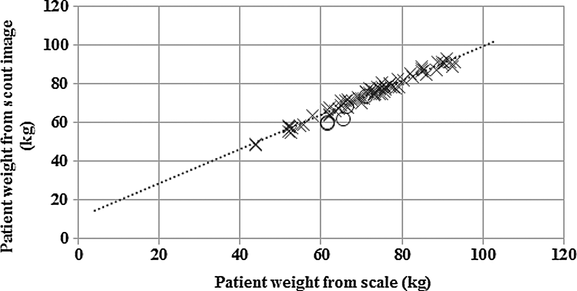
Figure 3 shows the patient weight as assessed by application of Equation A7 and using the system based calibration factor, csys. The correlation between the scout image-based assessment of the patient weight and that obtained by weighing on a scale is excellent with a squared correlation coefficient (R2) of 0.98. For the patients having a high-density hip implant, the weight was underestimated by about 10% for three studies and was within 2% for two studies.
The patient weight determined from patient scout images by using the calibration factor csys from the scanner system file, as a function of the patient weight. Crosses represent values obtained for 74 different patient scouts, and circles represent values obtained for 5 patients who had a metal hip implant. The linear fit has a slope of 0.88 and intercept of 10.9, with a correlation coefficient (R2) of 0.98.
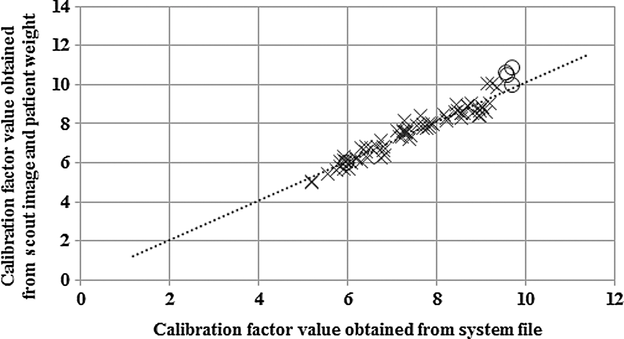
Figure 4 shows the relationship between the values of cW obtained from Equation A8, and the values of csys. The slope and intercept of the linear equation imply that the calibration factors determined from the two methods are in good agreement for most patients; however, there are larger deviations for patients having a metal hip implant.
The value of the calibration factor cW, determined using the scout image and patient weight (Equation 13), versus the calibration factor csys obtained from the scanner system file. Crosses represent values obtained for 74 different patient scouts, and circles represent values obtained for patients who had a metal hip implant. The linear fit has a slope of 1.01 and intercept of 0.027, with a correlation coefficient (R2) of 0.93.
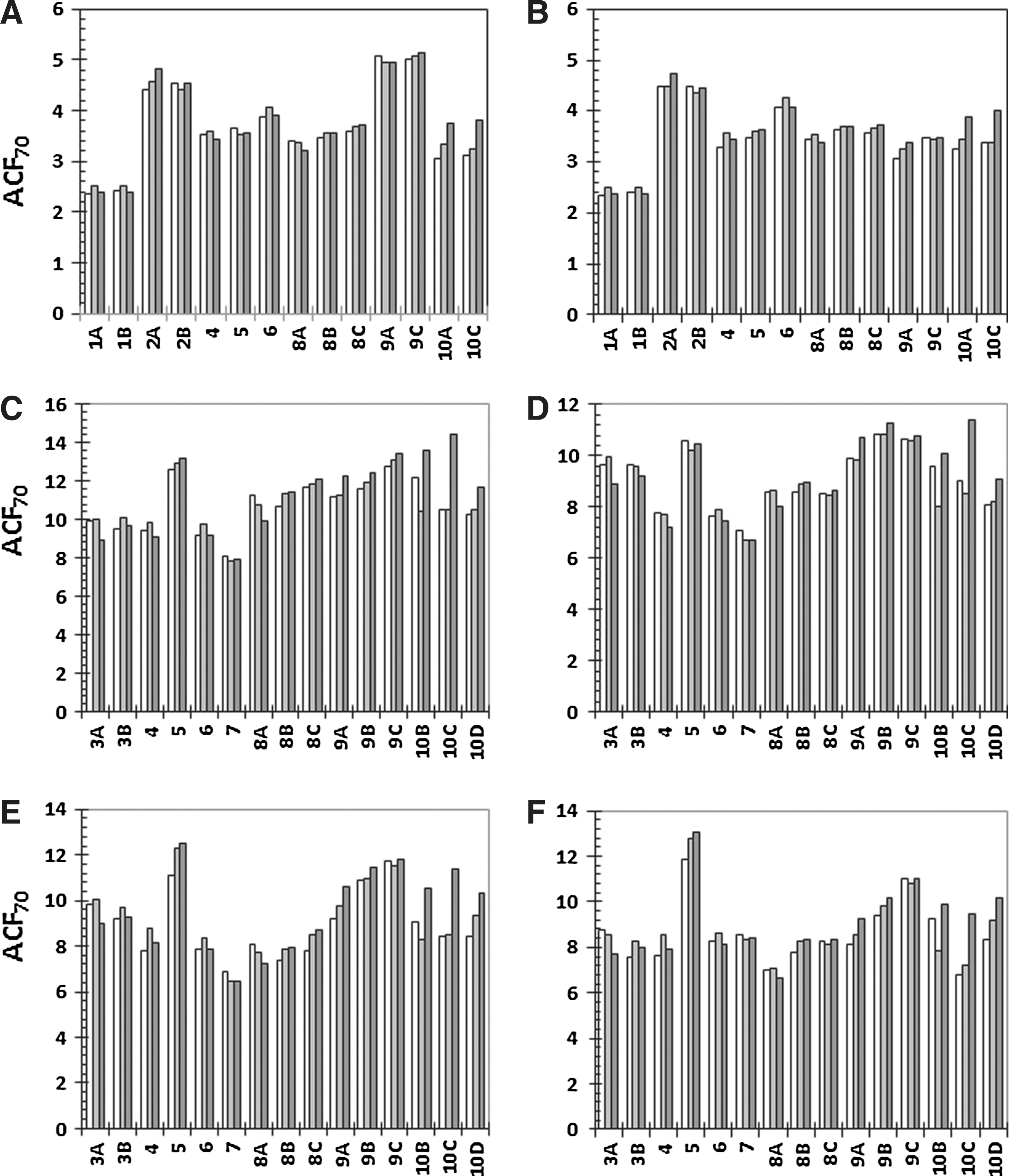
Figure 5 shows the values of the ACF for 70 keV in different organ ROIs. These were determined in three different AC maps; those determined from the CT studies (Equations 6–8 and 2), those obtained from the scout image and applying csys (Equations 4 and 2), and those obtained from the scout image and applying cw (Equations A8, 4 and 2). As the CT studies of the various patients cover different body parts, the different organs correspond to different patients. Patients 1–3 and 8–10 had multiple scout and CT measurements, and values from different occasions are designated A–D. Overall, the scout image-based values correspond well to those determined from CT. The largest deviations are obtained for patient 10 (studies 10A–10D), who has a hip implant, which made deviations increase, especially for the weight-based scout image calibration factor. Excluding patient 10, the maximum deviations from the CT-derived ACFs for the scout image-derived values using csys were 6.8%, 8.9%, 6.7%, −5.5%, 12.1%, and 11.2% for the left lung, right lung, liver, spleen, left kidney, and right kidney, respectively. The corresponding maximum deviations for the scout image-derived values using cw were 9.2%, 10.3%, −11.8%, 8.2%, 14.7%, and 13.6%, respectively. The obtained deviations did not correlate well with either the patient weight or BMI. Using the calibration factor \documentclass{aastex}\usepackage{amsbsy}\usepackage{amsfonts}\usepackage{amssymb}\usepackage{bm}\usepackage{mathrsfs}\usepackage{pifont}\usepackage{stmaryrd}\usepackage{textcomp}\usepackage{portland, xspace}\usepackage{amsmath, amsxtra}\pagestyle{empty}\DeclareMathSizes{10}{9}{7}{6}\begin{document}$${c^{\prime}} w$$\end{document} calculated without using a mixture of soft tissue and bone densities and attenuation coefficient values (Equation A9), the maximum deviations were −10.5%, −8.0%, −21.5%, −17.0%, −19.5%, and −20.7%, respectively (data not shown).
Values of the ACF for organ ROIs for 70 keV (ACF70) for patient studies 1–10 over (A): left lung, (B): right lung, (C): liver, (D): spleen, (E): left kidney, and (F): right kidney. White bars represent values determined from the CT-derived attenuation correction map; light gray bars represent scout-derived values using the calibration factor from the system file (cW), and dark gray bars represent scout-derived values with the calibration factor from the patient weight (cW). In patient study 10 the patient had a hip implant.
Table 1 shows the median and range of the ACFs obtained from the CT-based AC map (Equations 6–8 and 2) for different organ ROIs and photon energies. These were measured in the same set of studies as in Figure 5, excluding studies 10A–10D, since these were not considered to be representative of the overall accuracy. The value of the ACF decreased with increasing photon energy due to decreasing values of the mass attenuation coefficients. There was a notably wide range in the organ ACFs for different patients. Table 1 also shows the bias and precision (Equations 9–11) of the organ ACFs determined from the scout using csys (system-based) (Equations 4 and 2 or 5), and using cW (weight-based) (Equations A8 and 4, and 2 or 5). For energies of 208 keV and upward, the bias was below 4% for both scout image-based methods, for all organs evaluated. The standard deviations were higher using the weight-based calibration factor, presumably due to a variation in the definition of the patient contour in the determination of cW. For a photon energy of 208 keV, the maximum deviations from the CT-derived ACFs for the scout image-derived values using csys were 5.3%, 7.7%, 5.9%, −5.2%, −6.2%, and 5.5% for the left lung, right lung, liver, spleen, left kidney, and right kidney, respectively. The corresponding maximum deviations for the scout image-derived values based on cW were 8.4%, 8.2%, −9.5%, −6.6%, −9.2%, and −9.8%, respectively. For 245 and 364 keV, the maximum deviations were lower. For the calibration factor \documentclass{aastex}\usepackage{amsbsy}\usepackage{amsfonts}\usepackage{amssymb}\usepackage{bm}\usepackage{mathrsfs}\usepackage{pifont}\usepackage{stmaryrd}\usepackage{textcomp}\usepackage{portland, xspace}\usepackage{amsmath, amsxtra}\pagestyle{empty}\DeclareMathSizes{10}{9}{7}{6}\begin{document}$${c^{\prime}} w$$\end{document} calculated using Equation A9, the average bias obtained for the liver, spleen, and kidneys were −5.8%, −5.4%, and −4.9% for 208, 245, and 364 keV, respectively, which was thus higher than those obtained using cW (Table 1).
Values of the Attenuation Correction Factor in Organ ROIs for Different Photon Energies Based on CT Images (Median and Range) and Results of the Bias±Precision (Equations 9–11) in the Scout-Based ACFs Using the System Calibration Factor, csys (System-Based), and the Calibration Factor Determined from the Patient Weight, cW (Weight-Based)
CT-based values of the ACF in ROIs
Scout-based results bias±precision (%)
Energy (keV)
Median (min . max)
System-based
Weight-based
70 keV
Left Lung
3.6 (2.4 . 5.1)
1.5±3.3
0.56±3.8
(average X-ray energy)
Right Lung
3.5 (2.3 . 4.5)
3.0±3.4
2.3±3.6
Liver
10.9 (8.1 .12.8)
2.3±3.5
1.0±6.8
Spleen
9.1 (7.1 . 10.8)
0.039±2.8
−1.2±5.3
Left Kidney
8.6 (6.9 . 11.8)
3.9±5.9
2.7±8.3
Right Kidney
8.2 (7.0 . 11.9)
3.6±4.9
2.4±7.3
All organs
2.4±4.0
1.3±5.9
208 keV
Left Lung
2.4 (1.8 . 3.0)
2.4±2.1
2.1±2.8
(177-Lu)
Right Lung
2.3 (1.8 . 2.8)
3.5±2.1
3.1±2.4
Liver
5.1 (4.2 . 5.7)
1.2±3.0
0.36±5.0
Spleen
4.5 (3.9 . 5.1)
−1.2±2.1
−2.0±3.4
Left Kidney
4.4 (3.8 . 5.5)
0.57±3.9
−0.26±5.4
Right Kidney
4.3 (3.8 . 5.5)
0.49±3.3
−0.31±4.7
All organs
1.2±2.7
0.48±3.9
245 keV
Left Lung
2.3 (1.7 . 2.8)
2.3±2.0
2.0±2.7
(111-In)
Right Lung
2.2 (1.7 . 2.6)
3.4±2.0
2.9±2.3
Liver
4.7 (3.9 . 5.2)
1.3±2.9
0.43±4.7
Spleen
4.2 (3.6 . 4.7)
−1.0±2.0
−1.8±3.2
Left Kidney
4.1 (3.5 . 5.0)
0.57±3.7
−0.22±5.1
Right Kidney
4.0 (3.6 . 5.0)
0.50±3.1
−0.26±4.5
All organs
1.2±2.6
0.51±3.7
364 keV
Left Lung
2.1 (1.6 . 2.4)
1.8±1.7
1.5±2.3
(131-I)
Right Lung
2.0 (1.6 . 2.3)
2.7±1.7
2.4±1.9
Liver
3.8 (3.2 . 4.1)
0.82±2.5
0.10±4.1
Spleen
3.4 (3.0 . 3.8)
−1.2±1.8
−1.9±2.7
Left Kidney
3.4 (3.0 . 4.0)
0.10±3.2
−0.58±4.3
Right Kidney
3.3 (3.0 . 4.0)
0.06±2.7
−0.60±3.8
All organs
0.72±2.3
0.15±3.2
Values are obtained from 12 different patient studies for each organ.
ACF, attenuation correction factor.
To investigate the sensitivity of the method to deviations in the assessment of the representative X-ray energy, attenuation coefficient values for energies Et of 65 and 75 keV were applied instead of 70 keV in the determination of the CT-based AC map (Equations 6–8 and 2) and of the scout-derived AC map using cW (Equations A8, 4, and 2). For all organs, the CT-based ACFs increased by 4%–8% for 65 keV and decreased by 4%–7% for 75 keV. As a result of the changed CT-based values, the bias±precision (average for all organs) for the scout-derived values using csys were −3.4%±3.9% and 8.5%±4.1% for 65 and 75 keV, respectively, which, as compared to 2.4%±4.0% for 70 keV (Table 1), confirmed that the energy spectrum should be represented by an energy between 65 and 75 keV. For the scout-derived AC map using cW, the bias±precision was 3.0%±6.4%, and −0.3%±5.5% for 65 and 75 keV, respectively. Moderate variations in the assessment of the representative X-ray energy thus did not appreciably affect the accuracy of the scout-derived ACFs using cW.
Discussion
Activity quantification based on planar conjugate views is probably still the most widely used method for assessment of the absorbed dose in radionuclide therapy, and the attenuation correction is one of the most important corrections. In a previous work, a method for obtaining patient-specific attenuation correction maps from CT scout images was presented.7 To make CT scout images applicable for attenuation correction, a rescaling of the image intensity values using a calibration factor is required. In the previous work, the calibration factor was obtained from a scanner system file that is normally hidden from the user,7 and depending on the way the camera vendor's image acquisition software is designed, the factor may not be available. In this work, a new method for obtaining the calibration factor is presented, which is based on the patient weight. To our knowledge, this method is applicable to scout images from any X-ray system. In our center, we are currently using the weight-based calibration method for obtaining scout-based attenuation correction maps from different X-ray systems, since it is only the Discovery VH SPECT/CT system that allows for retrieval of the system-based calibration factor. In this work, this information was used to validate the weight-based calibration method. The results in Figure 4 show that the values of the calibration factors obtained from the system and from the weight-based method are indeed in good agreement.
Attenuation correction maps obtained from CT scout images have some important advantages. Owing to the higher photon flux, acquisition is faster than corresponding radionuclide measurements and can be performed postinjection, making it feasible for clinical studies. Also, the higher SNR of scout-based attenuation correction maps gives advantages. Although the average value of the ACF is probably not overly sensitive to the SNR for large ROIs such as the liver, a higher SNR will likely introduce less bias for smaller ROIs such as the kidneys and, in particular, most tumors. For pixel-based implementations of the conjugate view method (Equation 1), the SNR in the attenuation correction map will propagate linearly into the SNR of the activity image, important for the ability to outline organ ROIs used for activity quantification. Also, for lung ROIs, the scout image is useful for visualizing the lung contour, which is otherwise difficult to delineate on low-SNR radionuclide transmission images or scintillation camera images. An additional advantage of X-ray scout images is that the scatter fraction is very low compared to 57Co transmission images that are usually acquired in a geometry involving a broad beam and a large field-of-view detector. This makes the energy scaling between transmission and emission photon energies simpler, since tabulated narrow-beam linear attenuation coefficient scan be used.
The linear correlation shown in Figure 3 supports the idea that the patient weight can be estimated from scout images within the evaluated weight range. However, extrapolation toward lower patient weights gives an intercept of ∼11 kg. One reason for this offset is attenuation in the patient couch, which contributes to the image values in the scout image, S, in Equation A7. This attenuation should be corrected for and rightfully contributes to the attenuation correction map, but may produce a small error in the estimation of the patient weight. According to the product data of the Discovery VH SPECT/CT system, the couch is composed of low-attenuation carbon fiber. By measurement in CT studies of the couch thickness and its mass density (using Equation 7), and estimating the area of the couch that is within the patient contour, the weight of the couch that is included is estimated to 4 kg. This thus explains some of the offset, while other possible causes, such as X-ray scatter, are currently being investigated, since the offset may be of importance for pediatric patients. However, for adult patients, the current method works satisfactory, as judged from the results in Figures 4 and 5, and Table 1.
In addition to the calibration factor, the normalization of the scout image intensity also depends on the minimum and maximum values provided by the CT system (smin and smax, respectively, in Equation 4). For our system, the values in the acquired scout image, S0, range from −1000 to 3096, whereas for other systems, different dynamic ranges are used. Another parameter to be determined for the user is the representative energy of the X-ray system. In a previous study, this was determined to 70 keV for our system,7 consistent with that found by others using an 140 kVp CT system for attenuation correction.25 Moderate deviation, however, from the representative energy (65 or 75 keV instead of 70) was not found to be critical for the accuracy of the weight-based method.
Perhaps, the most important consideration for the weight-based calibration factor is the delineation of the patient contour. Initially, the contour was delineated by defining a gray-level threshold value by visual inspection, but due to the subjective and potentially non-reproducible nature of such an approach, an automated, noninteractive method was clearly needed. Although robust, the segmentation method suffers from some imprecision (Table 1), presumably as a result of the variable accuracy in the delineation of contours. More recent segmentation methods may be found useful for this application.
Of some importance for the scout-based method is the amount of cortical bone along the projection line, which entails a higher probability for photoelectric absorption and thus a higher value of the attenuation coefficient values. The currently used weighting factors in the image W are based on experimentally determined values from a comparison of a scout image and a whole-body CT scan for one patient, and it would be desirable to determine the weighing factors and their distribution, more thoroughly. The thickness of cortical bone in different skeletal regions has been investigated by Hough et al.20 From their data, the average thickness of all skeletal regions has been calculated to 1.81 mm, ranging from ∼0.5 mm up to 3–4 mm in the craniofacial bones and humeri. If the patient thickness over the head and legs is assumed to be 10 cm, the used value of W in these regions of 0.9 would provide a cortical bone thickness along the projection line of 1 cm. This would thus correspond to a photon traversal path length of two to three times the published values,20 which is considered to be in an acceptable range. Although the current method represents a practical compromise, it appears to be satisfactory in most cases, based on the reasonably low bias values obtained (Table 1). A refined method for estimating W could include acquisition of two scout images using different kilovolt settings, as is done is bone densitometry applications. By digital subtraction, skeletal structures can thus be highlighted and segmented, which could probably be used for an improved estimation of the image W. However, such a methodology would involve two patient X-ray scout scans.
The absorbed dose delivered to the patient during a scout scan has been estimated by data from the literature.26 For a 134-kVp X-ray system for bone densitometry with hardware filtering similar to our CT system, the effective dose for a whole-body scan was determined to be 0.38 μSv (mAs)−1; for our system (using a 2.5-mA tube current and a 120-second acquisition time), this corresponds to 114 μSv per scan. This can be compared to a standard planar chest X-ray giving a typical effective dose of 280 μSv per scan,26 and is small in comparison to the total-body absorbed dose given in radionuclide therapy.
For both scout image-based methods, increased deviations in the ACFs are obtained for patients having a metal hip implant. For the calibration method using cW, the replacement of the high-intensity pixel values over the hip implant by nearby pixel values enables an accurate contour segmentation, which is otherwise biased by the high-intensity focus. Possibly, the accuracy in the ACFs would be improved by modifying the fractions in the image W over the hip implant. However, the deviations are increased also when using csys, and the problem is likely inherent in the scout image information. A plausible explanation is that the wide range of the image intensities that must be covered by the image bit depth makes the digital quantization less accurate in cases with a very-high-intensity object.
The method used for determining attenuation correction maps from the 3D CT studies by calibration of Hounsfield numbers to mass density values originates from the methods commonly used in external beam therapy.27,28 Other methods for determining 3D attenuation maps from CT studies have been presented, for example by direct calibration to linear attenuation coefficients.29 The advantage with the formulation in Equations 6 and 7 is that a single calibration function can be used for obtaining 3D attenuation correction maps for any energy by a simple multiplication to the appropriate mass attenuation coefficient. Moreover, the same calibration function can be used for determination of the voxel mass for use in 3D dosimetry based on SPECT/CT.24
As discussed, attenuation correction can be applied on a pixel-by-pixel basis, following Equation 1, or on a regional basis. As a preliminary comparison of the effect of the application order for the attenuation correction, both methods were applied for the patient study shown in Figure 1. The ROI count rates in the scatter corrected anterior–posterior images were determined using the organ ROIs shown in Figure 1F, and attenuation correction was performed by an ACF determined from the scout image-based AC map. The largest difference from the results obtained by the pixel-based approach was −4% for the lungs. Concerning the influence on the statistical uncertainty in the estimated activity value, the SNR of the attenuation correction map is high compared to the SNR of the emission count rate images, and the order of the application of the attenuation correction has a minor influence on the final uncertainty. Importantly, however, the pixel-based approach has other advantages. First, scatter is heterogeneously distributed over the image and may be better estimated in an image-based correction scheme. Second, using Equation 1, the total body activity can be estimated at any time point, since the heterogeneous attenuation distribution over the body is taken into consideration. It should be noted that this is performed without prior information of the administered activity. In the LundADose program, the administered activity is used for an independent, patient-specific, quality control of the activity quantification, where the total body activity estimated from the first imaging time point (prevoiding) is usually within 5%–10%.13 Third, the pixel-based approach also allows for image-based pharmacokinetic analyses, generating parametric whole-body images of the uptake and washout rates of tissues and a separation of the activity in vascular and extravascular spaces.30
From Table 1, it is seen that the bias of the attenuation correction values from both scout image-based methods is <4% for all organs and all energies, whereas the imprecision is <6%. The maximum deviation obtained is ∼10%, of importance when dosimetry is performed on an individual basis. It is our belief that the obtained accuracy is still well within acceptable limits. The accuracy should be considered relative to the bias and imprecision of alternative methods for obtaining ACFs, which to our knowledge have not actually been evaluated in patients. It would be of interest to put the obtained deviations into relation to other sources of bias and imprecision in individual, planar-based assessments of the absorbed dose. However, there are numerous sources of uncertainty, including aspects in the organ activity quantification such as the scatter correction, the camera system sensitivity (i.e., counts-to-activity conversion factor), possible miss-registration between emission images and the attenuation correction map, the ROI delineation, the background overlap corrections, as well as aspects in the calculation of the radiation energy transport; for example, how well a particular patient is represented by the phantom used for calculation of S-values, and the assessment of the organ mass.31 The current analysis focused on one source of uncertainty, the accuracy of the attenuation correction, in planar imaging-based activity quantification. It thus represents only one component of the total uncertainty in such quantification; investigation of other factors affecting the total uncertainty is beyond the scope of this article.
Conclusions
A CT scout image-based method for obtaining attenuation correction maps for planar scintillation camera imaging activity quantitation has been developed. This method uses a scout image calibration derived from the patient weight. The accuracy of the obtained ACFs for different organs ROIs was evaluated by comparison to values derived from 3D CT studies, and good agreement was found with an average bias±precision of 0.5%±4% for photon energies above 208 keV.
Footnotes
Acknowledgments
The authors wish to acknowledge Karin Wingårdh, who performed the clinical patient studies. Also, we wish to acknowledge Dr. David Minarik, who presented the original method. Further, we would like to express our gratitude to the reviewers. This work was funded by the Swedish Research Council, Swedish Cancer Foundation, Gunnar Nilsson Foundation, Bertha Kamprad Foundation, Lund University Medical Faculty Foundation, and Lund University Hospital Donation Funds.
Disclosure Statement
There are no existing financial conflicts.
Appendix 1: Derivation of Weight-Based Calibration Factor
The assumption made is that the patient thickness, L(i, j), can be represented as a sum of two compartments, a soft tissue-equivalent compartment and a compartment of cortical bone, where spongiosa is assumed to belong to the former (Fig. 2). Denoting the portion of the mass density distribution ρ that belongs to the soft tissue-equivalent compartment as \documentclass{aastex}\usepackage{amsbsy}\usepackage{amsfonts}\usepackage{amssymb}\usepackage{bm}\usepackage{mathrsfs}\usepackage{pifont}\usepackage{stmaryrd}\usepackage{textcomp}\usepackage{portland, xspace}\usepackage{amsmath, amsxtra}\pagestyle{empty}\DeclareMathSizes{10}{9}{7}{6}\begin{document}$${\bold \rho}_{eq}^s$$\end{document}(g cm−3), and the thickness of cortical bone as Lb (cm), the line integral of \documentclass{aastex}\usepackage{amsbsy}\usepackage{amsfonts}\usepackage{amssymb}\usepackage{bm}\usepackage{mathrsfs}\usepackage{pifont}\usepackage{stmaryrd}\usepackage{textcomp}\usepackage{portland, xspace}\usepackage{amsmath, amsxtra}\pagestyle{empty}\DeclareMathSizes{10}{9}{7}{6}\begin{document}$${\bold \rho}_{eq}^s$$\end{document} can be described as a soft tissue-equivalent thickness, \documentclass{aastex}\usepackage{amsbsy}\usepackage{amsfonts}\usepackage{amssymb}\usepackage{bm}\usepackage{mathrsfs}\usepackage{pifont}\usepackage{stmaryrd}\usepackage{textcomp}\usepackage{portland, xspace}\usepackage{amsmath, amsxtra}\pagestyle{empty}\DeclareMathSizes{10}{9}{7}{6}\begin{document}$$\textbf{\textit{L}}_\textbf{\textit{eq}}^\textbf{\textit{s}}$$\end{document}(cm):
where ρs is the mass density of soft tissue18, with a value of 1.0 g cm−3. As the mass density of lung19 is 0.26 g cm−3, its contribution to \documentclass{aastex}\usepackage{amsbsy}\usepackage{amsfonts}\usepackage{amssymb}\usepackage{bm}\usepackage{mathrsfs}\usepackage{pifont}\usepackage{stmaryrd}\usepackage{textcomp}\usepackage{portland, xspace}\usepackage{amsmath, amsxtra}\pagestyle{empty}\DeclareMathSizes{10}{9}{7}{6}\begin{document}$$\textbf{\textit{L}}_{eq}^s (i , j)$$\end{document} is decreased compared to the physical thickness by a factor of 0.26/1.0. Similarly for spongiosa19, having a mass density of 1.18 g cm−3, the contribution to \documentclass{aastex}\usepackage{amsbsy}\usepackage{amsfonts}\usepackage{amssymb}\usepackage{bm}\usepackage{mathrsfs}\usepackage{pifont}\usepackage{stmaryrd}\usepackage{textcomp}\usepackage{portland, xspace}\usepackage{amsmath, amsxtra}\pagestyle{empty}\DeclareMathSizes{10}{9}{7}{6}\begin{document}$$\textbf{\textit{L}}_{eq}^s (i , j)$$\end{document} is increased compared to the physical thickness by a factor of 1.18/1.0 (Fig. 2).
A soft tissue- and bone-equivalent thickness distribution, \documentclass{aastex}\usepackage{amsbsy}\usepackage{amsfonts}\usepackage{amssymb}\usepackage{bm}\usepackage{mathrsfs}\usepackage{pifont}\usepackage{stmaryrd}\usepackage{textcomp}\usepackage{portland, xspace}\usepackage{amsmath, amsxtra}\pagestyle{empty}\DeclareMathSizes{10}{9}{7}{6}\begin{document}$$\textbf{\textit{L}}_{eq}^{sb}$$\end{document} (cm), is then defined as
where W is a matrix of weighing factors with a maximum value of one, describing the position-dependent fraction of the distribution \documentclass{aastex}\usepackage{amsbsy}\usepackage{amsfonts}\usepackage{amssymb}\usepackage{bm}\usepackage{mathrsfs}\usepackage{pifont}\usepackage{stmaryrd}\usepackage{textcomp}\usepackage{portland, xspace}\usepackage{amsmath, amsxtra}\pagestyle{empty}\DeclareMathSizes{10}{9}{7}{6}\begin{document}$$\textbf{\textit{L}}_{eq}^{sb}$$\end{document} that belongs to the soft tissue-equivalent compartment. The line integral of the entire mass density distribution ρ over the patient thickness is then approximated as follows:
where ρb is the mass density of cortical bone,17,18 and it has been assumed that the thickness of cortical bone, Lb, equals \documentclass{aastex}\usepackage{amsbsy}\usepackage{amsfonts}\usepackage{amssymb}\usepackage{bm}\usepackage{mathrsfs}\usepackage{pifont}\usepackage{stmaryrd}\usepackage{textcomp}\usepackage{portland, xspace}\usepackage{amsmath, amsxtra}\pagestyle{empty}\DeclareMathSizes{10}{9}{7}{6}\begin{document}$$\textbf{\textit{L}}_\textbf{\textit{eq}}^\textbf{\textit{sb}} [1 - \textbf{\textit{W}}]$$\end{document}. If the assumption is made that there is no cortical bone along the projection line, W equals one, and Equation A3 reduces to Equation A1.
The patient total body weight, mTB (g), can be described as the volume integral of the mass density over the patient volume. From Equation A3 this can be approximately described as:
where ΔiΔj is the pixel area (cm2), and the summation is performed over pixels with coordinates (i, j) that represent the patient in the image.
An approximate description of RE is obtained in a similar way, by seeing that the mass attenuation coefficient for different soft tissues can be well approximated by a constant soft tissue value, \documentclass{aastex}\usepackage{amsbsy}\usepackage{amsfonts}\usepackage{amssymb}\usepackage{bm}\usepackage{mathrsfs}\usepackage{pifont}\usepackage{stmaryrd}\usepackage{textcomp}\usepackage{portland, xspace}\usepackage{amsmath, amsxtra}\pagestyle{empty}\DeclareMathSizes{10}{9}{7}{6}\begin{document}$$( \mu / \rho ) _E^s$$\end{document}, so that
where \documentclass{aastex}\usepackage{amsbsy}\usepackage{amsfonts}\usepackage{amssymb}\usepackage{bm}\usepackage{mathrsfs}\usepackage{pifont}\usepackage{stmaryrd}\usepackage{textcomp}\usepackage{portland, xspace}\usepackage{amsmath, amsxtra}\pagestyle{empty}\DeclareMathSizes{10}{9}{7}{6}\begin{document}$$\mu_E^s$$\end{document} and \documentclass{aastex}\usepackage{amsbsy}\usepackage{amsfonts}\usepackage{amssymb}\usepackage{bm}\usepackage{mathrsfs}\usepackage{pifont}\usepackage{stmaryrd}\usepackage{textcomp}\usepackage{portland, xspace}\usepackage{amsmath, amsxtra}\pagestyle{empty}\DeclareMathSizes{10}{9}{7}{6}\begin{document}$$\mu_E^b$$\end{document}(cm−1) are the linear attenuation coefficients for soft tissue and cortical bone,18 respectively. Following Equation 4, an estimate of the image RE for E=Et is obtained from the scout image, S, as \documentclass{aastex}\usepackage{amsbsy}\usepackage{amsfonts}\usepackage{amssymb}\usepackage{bm}\usepackage{mathrsfs}\usepackage{pifont}\usepackage{stmaryrd}\usepackage{textcomp}\usepackage{portland, xspace}\usepackage{amsmath, amsxtra}\pagestyle{empty}\DeclareMathSizes{10}{9}{7}{6}\begin{document}$$\hat {R}_{Et} ( i , j ) = c \cdot \textbf{\textit{S}} ( i , j )$$\end{document}. Inserting into Equation A5 gives an estimate of \documentclass{aastex}\usepackage{amsbsy}\usepackage{amsfonts}\usepackage{amssymb}\usepackage{bm}\usepackage{mathrsfs}\usepackage{pifont}\usepackage{stmaryrd}\usepackage{textcomp}\usepackage{portland, xspace}\usepackage{amsmath, amsxtra}\pagestyle{empty}\DeclareMathSizes{10}{9}{7}{6}\begin{document}$$\textbf{\textit{L}}_{eq}^{sb}$$\end{document} as follows:
This in turn may be inserted to Equation A4, giving an estimate of the patient weight, \documentclass{aastex}\usepackage{amsbsy}\usepackage{amsfonts}\usepackage{amssymb}\usepackage{bm}\usepackage{mathrsfs}\usepackage{pifont}\usepackage{stmaryrd}\usepackage{textcomp}\usepackage{portland, xspace}\usepackage{amsmath, amsxtra}\pagestyle{empty}\DeclareMathSizes{10}{9}{7}{6}\begin{document}$$\hat{m}_{TB}$$\end{document}:
where the image indices for the matrix W have been temporarily omitted, for brevity.
By solving Equation A7 for c, the expression for the weight-based calibration factor cW is obtained:
For investigation of the sensitivity to the inclusion (or exclusion) of the partitioning distribution W in Equation A8, an expression where W(i,j) is set to unity everywhere is also given as \documentclass{aastex}\usepackage{amsbsy}\usepackage{amsfonts}\usepackage{amssymb}\usepackage{bm}\usepackage{mathrsfs}\usepackage{pifont}\usepackage{stmaryrd}\usepackage{textcomp}\usepackage{portland, xspace}\usepackage{amsmath, amsxtra}\pagestyle{empty}\DeclareMathSizes{10}{9}{7}{6}\begin{document}$$c{\prime}_W$$\end{document} according to the following equation:
Appendix 2: Practical Implementation Steps
References
1.
FlemingJS. A technique for the absolute measurement of activity using a gamma camera and computer. Phys Med Biol, 1979; 24:176.
2.
ThomasSR, MaxonHR, KereiakesJG. In vivo quantitation of lesion radioactivity using external counting methods. Med Phys, 1976; 03:253.
3.
SiegelJA, ThomasSR, StubbsJBet al.MIRD pamphlet no. 16: Techniques for quantitative radiopharmaceutical biodistribution data acquisition and analysis for use in human radiation dose estimates. J Nucl Med, 1999; 40:37S.
4.
Sjogreen-GleisnerK, DewarajaYK, ChiesaCet al.Dosimetry in patients with B-cell lymphoma treated with [90Y]ibritumomab tiuxetan or [131I]tositumomab. Q J Nucl Med Mol Imaging, 2011; 55:126.
5.
ChiesaC, BottaF, Di BettaEet al.Dosimetry in myeloablative (90)Y-labeled ibritumomab tiuxetan therapy: Possibility of increasing administered activity on the base of biological effective dose evaluation. Preliminary results. Cancer Biother Radiopharm, 2007; 22:113.
MinarikD, SjogreenK, LjungbergM. A new method to obtain transmission images for planar whole-body activity quantification. Cancer Biother Radiopharm, 2005; 20:72.
8.
GarkavijM, NickelM, Sjogreen-GleisnerKet al.177Lu-[DOTA0,Tyr3] octreotate therapy in patients with disseminated neuroendocrine tumors: Analysis of dosimetry with impact on future therapeutic strategy. Cancer, 2010; 116,4 Suppl:1084.
9.
LindénO, KurkusJ, GarkavijMet al.A novel platform for radioimmunotherapy: Extracorporeal depletion of biotinylated and 90Y-labeled rituximab in patients with refractory B-cell lymphoma. Cancer Biother Radiopharm, 2005; 20:457.
10.
MinarikD, Sjogreen-GleisnerK, LindenOet al.90Y Bremsstrahlung imaging for absorbed-dose assessment in high-dose radioimmunotherapy. J Nucl Med, 2010; 51:1974.
11.
ITT Visual Information Solutions. Interactive Data Language 6.4: Reference guide. Boulder, CO: ITT Visual Information Solutions, 2005.
12.
SjogreenK, LjungbergM, StrandSE. An activity quantification method based on registration of CT and whole-body scintillation camera images, with application to 131I. J Nucl Med, 2002; 43:972.
13.
SjogreenK, LjungbergM, WingardhK, MinarikD, StrandSE. The LundADose method for planar image activity quantification and absorbed-dose assessment in radionuclide therapy. Cancer Biother Radiopharm, 2005; 20:92.
14.
MinarikD, LjungbergM, SegarsP, GleisnerKS. Evaluation of quantitative planar 90Y bremsstrahlung whole-body imaging. Phys Med Biol, 2009; 54:5873.
15.
LjungbergM, StrandSE. A Monte Carlo program for the simulation of scintillation camera characteristics. Comput Methods Programs Biomed, 1989; 29:257.
16.
SjogreenK, LjungbergM, WingardhKet al.Registration of emission and transmission whole-body scintillation-camera images. J Nucl Med, 2001; 42:1563.
17.
International Commission on Radiation Units and Measurements. Report 44: Tissue Substitutes in Radiation Dosimetry and Measurement. Bethesda, MD: ICRU, 1989.
18.
Bibliography of Photon Total Cross Section (Attenuation Coefficient) Measurements (version 2.3). National Institute of Standards and Technology. 2003. www.nist.gov/pml/data/photon_cs/. 2012 May 18.
19.
International Commission on Radiation Units and Measurements. Report 46: Photon, Electron, Proton and Neutron Interaction Data for Body Tissues. Bethesda, MD: ICRU, 1992.
20.
HoughM, JohnsonP, RajonDet al.An image-based skeletal dosimetry model for the ICRP reference adult male—internal electron sources. Phys Med Biol, 2011; 56:2309.
21.
OtsuN. A Threshold selection method from gray-level histograms. IEEE Transact Syst Man Cybernet, 1979; SMC-9:62.
22.
MortelmansL, NuytsJ, Van PamelGet al.A new thresholding method for volume determination by SPECT. Eur J Nucl Med, 1986; 12:284.
Sjogreen-GleisnerK, RueckertD, LjungbergM. Registration of serial SPECT/CT images for three-dimensional dosimetry in radionuclide therapy. Phys Med Biol, 2009; 54:6181.
25.
KinahanPE, TownsendDW, BeyerTet al.Attenuation correction for a combined 3D PET/CT scanner. Med Phys, 1998; 25:2046.
26.
SteelSA, BakerAJ, SaundersonJR. An assessment of the radiation dose to patients and staff from a Lunar Expert-XL fan beam densitometer. Physiol Meas, 1998; 19:17.
27.
KnoosT, NilssonM, AhlgrenL. A method for conversion of Hounsfield number to electron density and prediction of macroscopic pair production cross-sections. Radiother Oncol, 1986; 5:337.
28.
VerhaegenF, DevicS. Sensitivity study for CT image use in Monte Carlo treatment planning. Phys Med Biol, 2005; 50:937.
29.
SeoY, WongKH, SunMet al.Correction of photon attenuation and collimator response for a body-contouring SPECT/CT imaging system. J Nucl Med, 2005; 46:868.
30.
Sjogreen GleisnerK, NickelM, LindénOet al.Parametric Images of antibody pharmacokinetics based on serial quantitative whole-body imaging and blood sampling. J Nucl Med, 2007; 48:1369.
31.
LassmannM, ChiesaC, FluxGet al.EANM Dosimetry Committee guidance document: Good practice of clinical dosimetry reporting. Eur J Nucl Med Mol Imaging, 2011; 38:192.
32.
PoludniowskiGG, EvansPM. Calculation of x-ray spectra emerging from an x-ray tube. Part I. electron penetration characteristics in x-ray targets. Med Phys, 2007; 34:2164.