A Voxel-Dose Algorithm of Heterogeneous Activity Distribution for Monte–Carlo Simulation of Radionuclide Therapy Dosimetry

Abstract

Purpose:

The organ or tumor activity is not uniform due to inhomogeneous expression/distributions of receptors/antigens and the nonuniform vascularization of the tumor tissue. However, most patient-specific three-dimensional Monte–Carlo methods for radionuclide dosimetry have dealt with quasi-homogeneous activity distributions. A voxel-by-voxel activity sample algorithm (VM) without artifacts is presented to calculate the dose of the heterogeneous activity distribution for radionuclide dosimetry.

Methods:

The source particle location is sampled according to the activity spatial distribution. The source particle weight is imparted by the relative activity concentration of its origination voxel. This algorithm is applied to calculate the dose volume histogram for multiple independent activity regions with Gauss diffusion activity distributions and then compared with the level partition method (LM). The minimal response and the mean tolerant initial total activity threshold required by tumor control probability and normal tissue complication probability for radioimmunotherapy (¹³¹I-RIT) also were evaluated by the voxel-by-voxel sample algorithm and the LM. The effective clearance half-time is assumed to be equal to its physical half-life (i.e., 8.02 days for ¹³¹I).

Results:

The result shows that the new algorithm is more consistent with the weighted superposition of the quasi-homogeneous activity distribution than the LM, especially for the multiple independent activity regions composed of different amounts of voxels. The new algorithm effectively avoids the leveling/binning artifacts to the heterogeneous activity distribution. The ¹³¹I-RIT simulation also showed that the minimal response initial total activity threshold of tumors will be much more than the mean tolerant initial total activity threshold of normal organs (e.g., kidney) with the activity heterogeneous grade deteriorating.

Conclusions:

A VM is presented to simulate the dose of the heterogeneous activity distribution for radionuclide dosimetry. The new algorithm effectively avoids the leveling/binning artifacts to the heterogeneous activity distribution.

Introduction

Accurate dose distribution calculation is very critical for radionuclide therapy to establish reliable dose-response relationships for target tissue and dose-toxicity relationships for normal tissue.¹ Patient-specific three-dimensional (3-D) Monte–Carlo methods for radionuclide dosimetry have been extensively implemented.^1

–9 Generally, these works have simulated the organ or tissue source assuming activity homogeneous distribution.^{4
–6,8
–10} However, radiopharmaceuticals are observed to be generally distributed nonuniformly over the entire range of spatial levels, ranging from the organ to the sub-cell,¹¹ which will lead to a nonuniform absorbed dose distribution. Some works have realized the heterogeneously distributed activity calculation by dividing the distribution into several homogeneous levels to calculate their dose distribution.^4,7,12 For example, Song et al.⁷ divided activity into 5, 10, or 20 equally sized activity bins on the 3-D lung activity map. The voxels belonging to the same bin on the activity map were merged on the density map and assigned the same universe number in the MCNP4B input file. However, this partition method could bring up artifacts if the bin/level number is not sufficient,⁷ and the artifacts have not been evaluated for the situation of concurrent multiple independent activity regions. The remarkably different activity proportion in organs or tissues is very common in clinics for activity injections and metabolism. For example, Dewaraja et al.¹ have shown that the activity proportion is 1 for tumor, and 0.28 for liver and lung, respectively, based on a real imaging study with radioimmunotherapy (¹³¹I RIT).

The EGSnrc code¹³ is an extended and improved version of EGS4. It incorporates significant improvements in the implementation of the condensed history technique for the simulation of the charged particle transport and better low energy cross-sections. EGSnrc is an open source program and under persisting updates. EGSnrc has also been applied in patient-specific 3-D plans for radionuclide therapy¹⁴ using the level partition method (LM).⁷ Hadid et al. calculated the specific absorbed fractions (SAFs) of energy for photons and electrons based on ICRP/ICRU reference phantoms using EGSnrc, in which only the uniformly distributed organ source was simulated.¹⁰

This work presents a voxel-by-voxel activity sample algorithm (VM) that assesses the dose calculation of the heterogeneous activity distribution for radionuclide dosimetry. The source particle location is sampled according to the activity spatial distribution. The source particle weight is imparted by the relative activity concentration of its origination voxel. The new algorithm is implemented into EGSnrc user code DOSXYZnrc based on a CT-based phantom. The simulated dose volume histograms (DVHs) of the VM has been compared with those of the LM based on an extensively distributed activity map from realistic image activity data for radioisotope ¹³¹I RIT. The more complex heterogeneous activity distribution of Gauss diffusion is also investigated by the LM and the voxel-by-voxel sample algorithm which show the artifact caution of the LM.

Materials and Methods

The following sections will first introduce the VM. To compare the simulated result of VM with other methods, the superposition method (SM) and the LM also will be introduced and simulated. A typical heterogeneous activity distribution example from a real imaging study with ¹³¹I RIT¹ is chosen to show the simulation ability of three methods to the heterogeneous activity distribution. The implementation of the three activity sample algorithms into EGSnrc user code DOSXYZnrc based on a CT-based phantom will be described. The required simulation parameters and the calculation formula of the cumulative activity and the initial activity also will be introduced.

Voxel-by-voxel activity sample algorithm

The VM regards each voxel with non-zero activity as an independent, homogeneous, and equal-volume voxel source. The weight of each voxel source W_Voxel equals the relative activity A_RVoxel , which can be obtained by the voxel activity A_Voxel divided by the total activity of all the voxel sources. The activity is normalized to be such that the summed weight (i.e., sample probability) of all the voxel sources should be 100%. The origination position (or coordinate) of any emitter is homogeneously and randomly sampled in the activity distribution region. As long as the activity of its origination voxel is larger than zero, then this origination position sample is a successful one. The emitter will start transporting from here in an isotropical manner. The emitter weight W_Emitter equals the weight of its origination voxel. To accelerate the position sample, the minimal and maximal boundaries of the activity distribution are hunted for and used to reduce the sample extent. Figure 1 shows the algorithm flowchart.

FIG. 1.

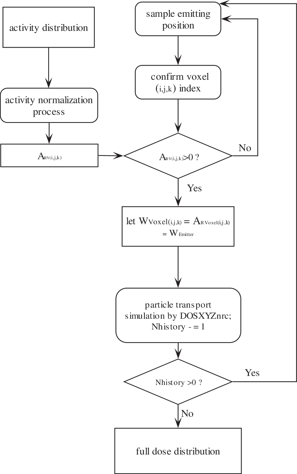
The flowchart of the VM. VM, voxel-by-voxel activity sample algorithm; SM, superposition method; LM, level partition method.

By assuming each voxel with non-zero activity as an independent homogeneous and equal-volume voxel source, the dose of the (i, j, k) voxel, dose_i,j,k is, \documentclass{aastex}\usepackage{amsbsy}\usepackage{amsfonts}\usepackage{amssymb}\usepackage{bm}\usepackage{mathrsfs}\usepackage{pifont}\usepackage{stmaryrd}\usepackage{textcomp}\usepackage{portland, xspace}\usepackage{amsmath, amsxtra}\pagestyle{empty}\DeclareMathSizes{10}{9}{7}{6}\begin{document} \begin{align*}dose_{i , j , k} = \mathop\sum_{i{\prime} = 1 , j{ \prime} = 1 , k{ \prime} = 1}^{N_i N_j N_k} W_{Voxel {( {i{\prime} , j{ \prime} , k{ \prime} ) }}} \cdot d_{Voxel ( i , j , k \leftarrow i{ \prime} , j{ \prime} , k{ \prime} ) } \tag{1}\end{align*}\end{document}

In Eq. 1, \documentclass{aastex}\usepackage{amsbsy}\usepackage{amsfonts}\usepackage{amssymb}\usepackage{bm}\usepackage{mathrsfs}\usepackage{pifont}\usepackage{stmaryrd}\usepackage{textcomp}\usepackage{portland, xspace}\usepackage{amsmath, amsxtra}\pagestyle{empty}\DeclareMathSizes{10}{9}{7}{6}\begin{document}$$d_{Voxel ( i , j , k \leftarrow i{ \prime} , j{ \prime} , k{\prime} )}$$\end{document} is the dose contribution from the (i′, j′, k′) voxel source to the (i, j, k) voxel. The weight of the (i′, j′, k′) voxel source \documentclass{aastex}\usepackage{amsbsy}\usepackage{amsfonts}\usepackage{amssymb}\usepackage{bm}\usepackage{mathrsfs}\usepackage{pifont}\usepackage{stmaryrd}\usepackage{textcomp}\usepackage{portland, xspace}\usepackage{amsmath, amsxtra}\pagestyle{empty}\DeclareMathSizes{10}{9}{7}{6}\begin{document}$$W_{Voxel ({i{ \prime} , j{ \prime} , k{ \prime}} ) }$$\end{document} is \documentclass{aastex}\usepackage{amsbsy}\usepackage{amsfonts}\usepackage{amssymb}\usepackage{bm}\usepackage{mathrsfs}\usepackage{pifont}\usepackage{stmaryrd}\usepackage{textcomp}\usepackage{portland, xspace}\usepackage{amsmath, amsxtra}\pagestyle{empty}\DeclareMathSizes{10}{9}{7}{6}\begin{document}\begin{align*}W_ { Voxel { ( i { \prime } , j { \prime } , k { \prime } ) } } = \frac { A_ { Voxel ( { i { \prime } , j { \prime } , k { \prime } } ) } } { \mathop\sum \limits_ { i { \prime } = 1 , j { \prime } = 1 , k { \prime } = 1 } ^ { N_i N_j N_k } A_ { Voxel ( { i { \prime } , j { \prime } , k { \prime } ) } } } \tag { 2 } \end{align*}\end{document}

In Eq. 2, \documentclass{aastex}\usepackage{amsbsy}\usepackage{amsfonts}\usepackage{amssymb}\usepackage{bm}\usepackage{mathrsfs}\usepackage{pifont}\usepackage{stmaryrd}\usepackage{textcomp}\usepackage{portland, xspace}\usepackage{amsmath, amsxtra}\pagestyle{empty}\DeclareMathSizes{10}{9}{7}{6}\begin{document}$$A_{Voxel ( {i{ \prime} , j{ \prime} , k{ \prime} ) }}$$\end{document} is the activity of the (i′, j′, k′) voxel, \documentclass{aastex}\usepackage{amsbsy}\usepackage{amsfonts}\usepackage{amssymb}\usepackage{bm}\usepackage{mathrsfs}\usepackage{pifont}\usepackage{stmaryrd}\usepackage{textcomp}\usepackage{portland, xspace}\usepackage{amsmath, amsxtra}\pagestyle{empty}\DeclareMathSizes{10}{9}{7}{6}\begin{document}$$\sum\nolimits_{i{ \prime} = 1 , j{ \prime} = 1 , k{ \prime} = 1}^{N_i N_j N_k} A_{Voxel ( {i{ \prime} , j{ \prime} , k{ \prime}) }}$$\end{document} is the total activity of all the voxels.

The weight of the nth emitter originating from the (i′, j′, k′) voxel source is \documentclass{aastex}\usepackage{amsbsy}\usepackage{amsfonts}\usepackage{amssymb}\usepackage{bm}\usepackage{mathrsfs}\usepackage{pifont}\usepackage{stmaryrd}\usepackage{textcomp}\usepackage{portland, xspace}\usepackage{amsmath, amsxtra}\pagestyle{empty}\DeclareMathSizes{10}{9}{7}{6}\begin{document}\begin{align*}W_{Emitter ( n ) } = W_{Voxel ( {i{ \prime} , j{ \prime} , k{ \prime} ) }} \tag{3}\end{align*}\end{document}

Thus, this algorithm replaces the sub-source (i.e., voxel sources here) weight with the weight of the nth emitter to scale its dose deposition.

Superposition method

The SM of homogeneous organ or tumor sources (i.e., sub-sources) is simulated based on the quasi-homogeneous activity distribution, which means that the activity is homogeneous in organ or tumor regions, but inhomogeneous in different organ or tumor regions. The dose of the (i, j, k) voxel, does_i,j,k , is the dose combination of all the sub-sources (i.e., organs with activity more than zero) in this voxel. The organ local activity divided by the total local activity of all source organs represents the relative weight of different sub-sources. Thus, dose_i,j,k is \documentclass{aastex}\usepackage{amsbsy}\usepackage{amsfonts}\usepackage{amssymb}\usepackage{bm}\usepackage{mathrsfs}\usepackage{pifont}\usepackage{stmaryrd}\usepackage{textcomp}\usepackage{portland, xspace}\usepackage{amsmath, amsxtra}\pagestyle{empty}\DeclareMathSizes{10}{9}{7}{6}\begin{document}\begin{align*}dose_{i , j , k} = \mathop\sum_{m = 1}^{N_m} W_{Rm} \cdot d_{i , j , k \leftarrow m} \tag{4}\end{align*}\end{document}

In Eq. 4, d_i,j,k _←m is the dose contribution from the mth sub-source to the (i, j, k) voxel. The weight of the mth sub-source region, W_Rm , is \documentclass{aastex}\usepackage{amsbsy}\usepackage{amsfonts}\usepackage{amssymb}\usepackage{bm}\usepackage{mathrsfs}\usepackage{pifont}\usepackage{stmaryrd}\usepackage{textcomp}\usepackage{portland, xspace}\usepackage{amsmath, amsxtra}\pagestyle{empty}\DeclareMathSizes{10}{9}{7}{6}\begin{document}\begin{align*}W_ { Rm } = \frac { A_m } { \mathop\sum \limits_ { m { \prime } = 1 } ^ { N_m } A_ { m { \prime } } } \tag { 5 } \end{align*}\end{document}

In Eq. 5, A_m is the activity of the mth sub-source, and \documentclass{aastex}\usepackage{amsbsy}\usepackage{amsfonts}\usepackage{amssymb}\usepackage{bm}\usepackage{mathrsfs}\usepackage{pifont}\usepackage{stmaryrd}\usepackage{textcomp}\usepackage{portland, xspace}\usepackage{amsmath, amsxtra}\pagestyle{empty}\DeclareMathSizes{10}{9}{7}{6}\begin{document}$$\sum \nolimits_{m{ \prime} = 1}^N A_{m{ \prime}}$$\end{document} is the total activity of all the sub-sources.

The SM of the voxel dose, something similar to the Medical Internal Radiation Dose (MIRD) methodology,¹⁵ regards each organ or tissue as an independent sub-source unit, and the activity of each voxel in the same organ or tissue is the same. Thus, the SM is not suitable for simulation of the activity heterogeneous distribution in the organ or tumor region, such as the Gauss diffusion.

Level partition method

The LM equally divides the whole heterogeneous activity distribution into different activity bins (i.e., levels) from the minimum to the maximum voxel activity. The bin or level median value is assumed to be the level activity value. The relative level activity (A_Rl ) of the lth level source can be obtained as \documentclass{aastex}\usepackage{amsbsy}\usepackage{amsfonts}\usepackage{amssymb}\usepackage{bm}\usepackage{mathrsfs}\usepackage{pifont}\usepackage{stmaryrd}\usepackage{textcomp}\usepackage{portland, xspace}\usepackage{amsmath, amsxtra}\pagestyle{empty}\DeclareMathSizes{10}{9}{7}{6}\begin{document}\begin{align*}A_ { Rl } = \frac { A_l } { \mathop\sum \limits_ { l { \prime } = 1 } ^ { N_l } A_ { l { \prime } } } \tag { 6 } \end{align*}\end{document}

In Eq. 6, A_l is the level median activity of the lth level source, \documentclass{aastex}\usepackage{amsbsy}\usepackage{amsfonts}\usepackage{amssymb}\usepackage{bm}\usepackage{mathrsfs}\usepackage{pifont}\usepackage{stmaryrd}\usepackage{textcomp}\usepackage{portland, xspace}\usepackage{amsmath, amsxtra}\pagestyle{empty}\DeclareMathSizes{10}{9}{7}{6}\begin{document}$$\sum \nolimits_{l{ \prime} = 1}^{N_l} A_{l{ \prime}}$$\end{document} is the total median activity of all the non-zero level sources.

Thus, the dose of the (i,j,k) voxel, dose_i,j,k , is \documentclass{aastex}\usepackage{amsbsy}\usepackage{amsfonts}\usepackage{amssymb}\usepackage{bm}\usepackage{mathrsfs}\usepackage{pifont}\usepackage{stmaryrd}\usepackage{textcomp}\usepackage{portland, xspace}\usepackage{amsmath, amsxtra}\pagestyle{empty}\DeclareMathSizes{10}{9}{7}{6}\begin{document}\begin{align*}dose_{i , j , k} = \mathop\sum_{l = 1}^{N_l} A_{Rl} \cdot d_{i , j , k \leftarrow l} \tag{7}\end{align*}\end{document}

In Eq. 7, d_i,j,k←l is the dose contribution from the lth level source to the (i, j, k) voxel.

A typical activity distribution

A typical activity distribution from a real imaging study with ¹³¹I RIT¹ has been simulated. The activity relative concentrations in different regions are chosen to be tumor, 1; kidneys, 0.80; liver, 0.28; spleen, 0.52; lung, 0.28; heart, 0.48; blood pool, 0.48; and rest of the body, 0.04. This activity distribution is a quasi-homogeneous activity one, which is similar to Gauss distribution with a sigma of 0.0 at the organ scale (called D 0.0, hereafter). To illustrate the simulation ability of the three methods to the heterogeneous activity distribution, Gauss diffusion cases of the quasi-homogeneous activity distribution source (called D 0.3 for Gauss distribution with a sigma of 0.3; D 0.6 for Gauss distribution with a sigma of 0.6) were also simulated. The tumor is assumed to be a 135 mL sphere (corresponding to the radius of 3.18 cm) located in the abdomen.

Simulation parameters

The VM algorithm is implemented into EGSnrc¹³ user code DOSXYZnrc based on the CT-based Zubal phantom.¹⁶ The phantom is a 128×128×243 matrix with a 4 mm voxel size in all directions. There are 68 segmented organs or tissues in the whole Zubal phantom. Their materials were produced by PEGS4 (preprocessor for EGS) to represent critical organs or tissues. PEGS4 is a stand-alone utility program written in Mortran language aiming at generating material data for the EGS code. The lower cutoff energies for charged particle transport (AE) and photon transport (AP) are 0.512 MeV and 0.001 MeV, respectively, which correspond to the electron and photon cutoff kinetic energies of 1 keV. Both the globe electron and photon cutoffs (ECUT and PCUT) were set to be 1 keV. The PRESTA-II algorithm has been employed for the electron step control, which takes into account the lateral and the longitudinal correlations in a condensed history step.

Most organ or tissue material compositions are from the ASTAR and PSTAR Materials Website (http://physics.nist.gov/cgi-bin/Star/compos.pl?ap) as long as it is provided. The rest is assumed to be the default four materials (air, lung, soft tissue, and bone). To make the dose postprocess convenient, each organ or tissue is named by one of the material names. For example, the voxel belonging to the lung organ was given the material number of LungICRP. The voxel belonging to the kidney organ was given the material number of Kidney. A C++ utility was developed to convert Zubal original binary format to the required format of the DOSXYZnrc egsphant file.

To simplify the energy spectrum simulation of radionuclide emitters, a suit of single β spectra for different β-radionuclides by putting together a compilation of β-radionuclide spectra¹⁷ [www.doseinfo-radar.com/RADARDecay.html] was used here to compare different algorithms. Although ¹³¹I decay can emit β⁻, Auger e⁻, X-ray, and γ, a compilation of β spectra can be used to represent their integrative effect as far as the organ scale is concerned, which is very common in clinics. To obtain the reliable statistical uncertainty (<1% in source organs), 4×10⁸ primary particles were simulated for the activity distribution source using an Intel(R) Xeon(R) E5620 Power (CPU 2.40 GHz, 3.0 GB memory) under Windows system. It used about 16 hours for ¹³¹I.

Cumulative activity and initial activity

The effective clearance half-time of the radionuclide is assumed to be equal to its physical half-life (i.e., 8.02 days for ¹³¹I). According to the mono-exponential model assuming instantaneous activity uptake,¹⁸ the total accumulative dose TD_i,j,k in the (i, j, k) voxel is, \documentclass{aastex}\usepackage{amsbsy}\usepackage{amsfonts}\usepackage{amssymb}\usepackage{bm}\usepackage{mathrsfs}\usepackage{pifont}\usepackage{stmaryrd}\usepackage{textcomp}\usepackage{portland, xspace}\usepackage{amsmath, amsxtra}\pagestyle{empty}\DeclareMathSizes{10}{9}{7}{6}\begin{document}\begin{align*}TD_ { i , j , k } = \frac { T_ { ec } } { \ln 2 } \times A_0 \times dose_ { i , j , k } \tag { 8 } \end{align*}\end{document}

In which A ₀ is the initial injected activity to the whole body if dose_i,j,k is assumed to be the absorbed dose in the (i, j, k) voxel by one injected decay unit (i.e., Bq). T_ec is the effective clearance half-time. Thus, the initial injected activity A ₀ can be estimated by \documentclass{aastex}\usepackage{amsbsy}\usepackage{amsfonts}\usepackage{amssymb}\usepackage{bm}\usepackage{mathrsfs}\usepackage{pifont}\usepackage{stmaryrd}\usepackage{textcomp}\usepackage{portland, xspace}\usepackage{amsmath, amsxtra}\pagestyle{empty}\DeclareMathSizes{10}{9}{7}{6}\begin{document}\begin{align*}A_0 = \frac { TD_ { i , j , k } \times \ln 2 } { dose_ { i , j , k } \times T_ { ec } } \tag { 9 } \end{align*}\end{document}

As an excretive organ, the renal toxicity is often a concern in therapeutic molecular nuclear medicine, such as peptide-mediated receptor targeting.^18,19 If the minimal dose threshold to kill tumors is assumed to be 60 Gy and the mean dose threshold to protect kidney function is assumed to be 28 Gy (i.e., dose for a probability of 50% injury within 5 years for whole-kidney irradiation²⁰), the minimal response initial total activity threshold of the tumor and the mean tolerant initial total activity threshold considering the kidney based on Eq. 9 can be calculated. The therapeutic efficacy parameters such as tumor control probability (TCP) strongly depend on the survival clonogen number. Even one survival clonogen will decrease the TCP from 100% to 37% according to TCP's Poisson definition [i.e., TCP=exp (-N), N is the number of survival clonogens]. Thus, the minimal response initial total activity threshold of the tumor is obtained by setting the minimal voxel dose at 60 Gy, and the mean tolerant initial total activity threshold for the kidney is obtained by setting the averaged voxel dose at 28 Gy.

Results

The three-method comparison of multiple source regions with different activity distributions of D 0.0, 0.3, and 0.6 was investigated. Figure 2A shows the DVH comparison of three methods for one activity region (i.e., tumor). The level number of LM is 10⁵. The results show that three of them are very consistent for one region source. Figure 2B shows the effect of the level number on the DVH of the Level Method. Generally, 10² levels are enough to make the profile steady for D 0.6. Figure 3A shows the DVH comparison of three methods for two activity regions (i.e., the relatively activity concentrations are 1 for tumor and 0.8 for kidney). The level number of LM is still 10⁵. There is a slight inconsistency between LM with VM and SM even for D 0.3 and D 0.6. Figure 3B shows the effect of the level number on DVH by LM. Generally, 10² levels are also enough to make the profile steady for D 0.6 for two independent activity regions.

FIG. 2.

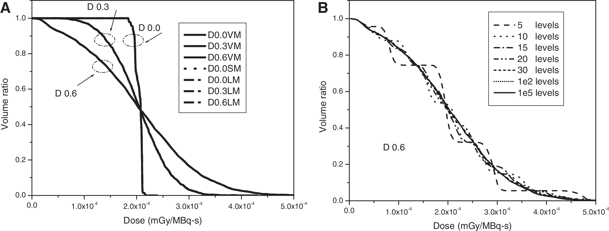
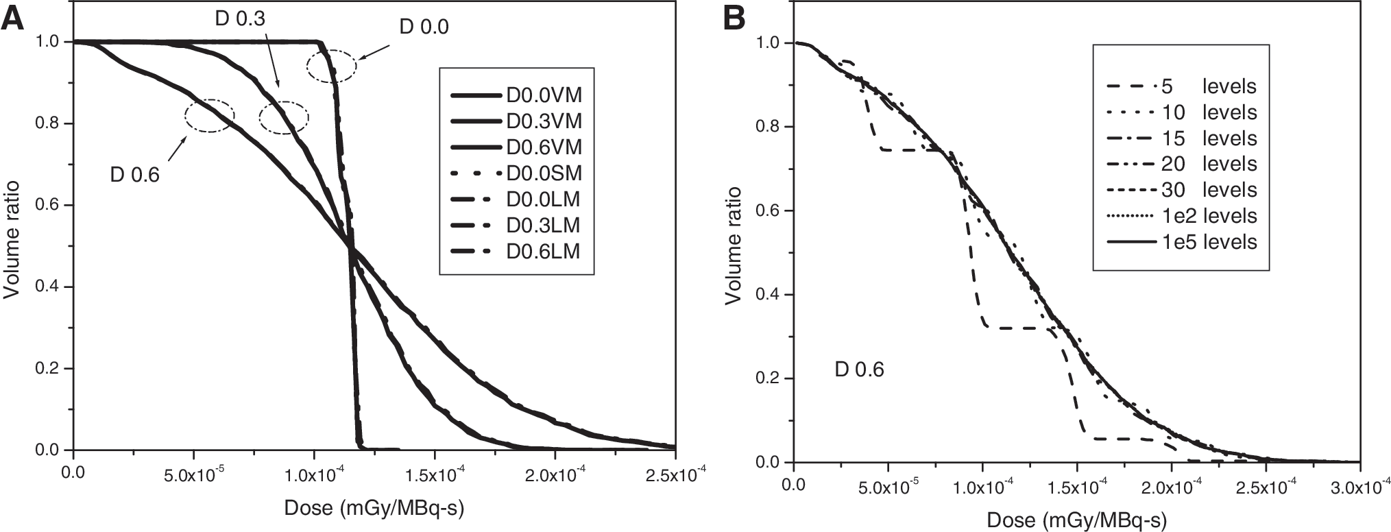
Comparison of three methods for one independent activity region (tumor), (A) DVH comparison; (B) the effect of the level number on DVH for D 0.6 by LM.

FIG. 3.

Comparison of three methods for two independent activity regions (tumor and kidney), (A) DVH comparison; (B) the effect of the level number on DVH for D 0.6 by LM.

Figure 4A shows the DVH comparison of three methods for three activity regions (i.e., 1 for tumor, 0.8 for kidney, and 0.28 for liver). The level number of LM still is 10⁵. There is some inconsistency between LM with VM and SM for D 0.0. There are also differences between VM and LM for D 0.3 and 0.6. Figure 4B shows the effect of the level number on DVH by LM. Generally, 10³ levels are enough for D 0.6. However, if the level number is not sufficient, then the averaged dose in tumors will offset to a low value. Figure 5 shows the DVH comparison of three methods for four independent activity regions (i.e., 1 for tumor, 0.8 for kidney, 0.28 for liver, and 0.28 for lung). The differences between VM and SM and LM are enlarged much more than those of Figure 4A. As for D 0.0, the VM and SM are consistent; however, LM offsets to a higher value. As for D 0.3 and D 0.6, LM also offsets a little to a higher value than VM. However, if the lung source is replaced by the spleen source, that is, 1 for tumor, 0.8 for kidney, 0.28 for liver, and 0.52 for spleen, then their difference will be similar to the differences observed in Figure 4A. The effect of the level number on DVH for four independent activity regions is similar to those of Figure 4B, and seven independent activity regions (i.e., 1 for tumor, 0.8 for kidney, 0.28 for liver, 0.48 for heart, 0.28 for lung, 0.48 for blood, and 0.52 for spleen) show the same features as those of Figures 5 and 4B; thus, they are not repeated here. If three independent activity regions are 1 for tumor, 0.8 for kidney, and 0.52 for spleen, then their DVH will be similar to Figure 3A and B.

FIG. 4.

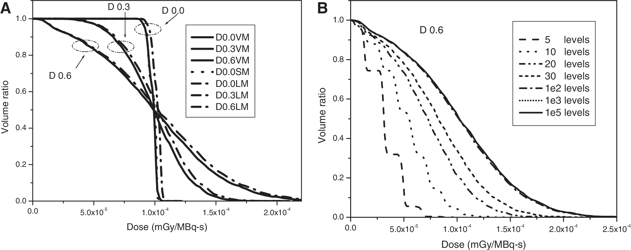
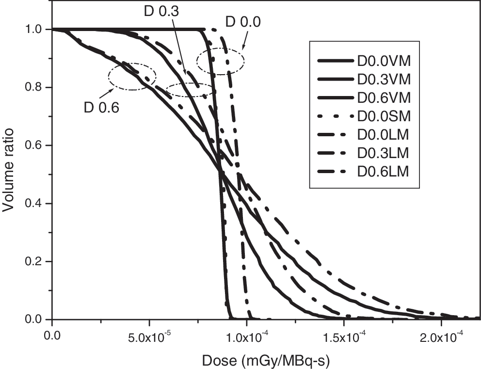
Comparison of three methods for two independent activity regions (tumor, kidney, and liver), (A) DVH comparison; (B) the effect of the level number on DVH for D 0.6 by LM.

FIG. 5.

The DVH comparison of three methods for four independent activity regions (tumor, kidney, liver, and lung).

To explore the reason for the differences of three methods for multiple independent activity regions, the organ weights for D 0.0 are investigated. Figure 6 shows that VM and SM have the same weight, but the weights of LM are a little different from those of VM and SM. Basically, one feature shows in common that the weight of the organ composed of relatively more voxels will be a little lower than that of SM, whereas the weight of the organ composed of relatively less voxels will be a little higher than SM. It is relative for the same source organ to have the lower or higher weight. For example, for two activity regions (tumor and kidney), the tumor weight is a little higher, and the kidney weight is a little lower than the original value (i.e., SM). However, as for three activity regions, the voxel number of the liver is a lot more than those of the tumor or kidney; thus, the kidney weight is a little higher than that of the SM. Four activity regions show similar features. The features could be due to the partition process artifact of the Level Method to the original weight (or activity) distribution. If the level number is not enough for the complex weight distribution, then the voxel weight will be classified into unsuitable weight bins or levels, so that the result will bias similar to Figures 2B, 3B, and 4B.

FIG. 6.

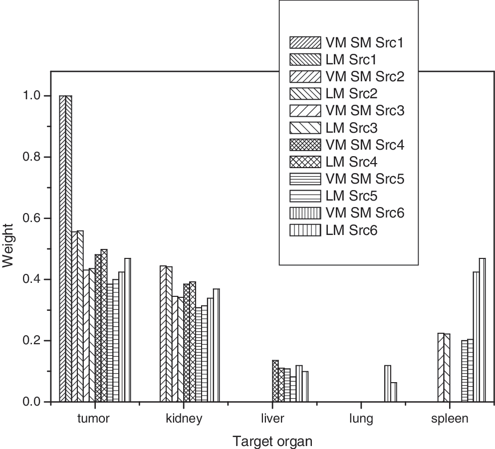
The organ weight in three methods for multiple independent activity regions of D 0.0. The voxel numbers of tumor, kidney, liver, lung and spleen in Zubal phantom are 2103, 7618, 29277, 62374 and 5568, respectively. Note: Src 1: tumor source; Src 2: tumor-kidney source; Src 3: tumor-kidney-spleen source; Src 4: tumor-kidney-liver source; Src 5: tumor-kidney-liver-spleen source; Src 6: tumor-kidney-liver-lung source.

Figure 7A, B shows the similar S factor of the tumor and kidney with sigma of 0.0, 0.3, and 0.6 for different activity regions. It is called the similar S factor, as it is not similar to the conventional S factor with only one source region. Figure 7A shows the comparison of VM with SM for varied activity heterogeneous distribution. Figure 7B shows that of the LM with SM. SM only simulates the quasi-homogeneous activity distribution source (D 0.0). As for D 0.0, the results of VM and SM are very similar, whereas the mean, minimum, and maximum of LM with SM and VM offset a little while including liver or lung sources. For the heterogeneous activity distribution source (D 0.3 and D 0.6), although the mean similar S factors of D 0.0, D 0.3, and D 0.6 for VM and LM are very similar, their minimum and maximum similar S factor are very different. The gap between the minimum and the maximum enlarges with the heterogeneous grade deteriorating. However, the activity heterogeneous grade does not exhibit an obvious influence on the mean difference of VM and LM. For example, there is about 3.87% difference for D 0.0 and 3.21% difference for D 0.6 in the tumor for the tumor-kidney-liver activity regions.

FIG. 7.

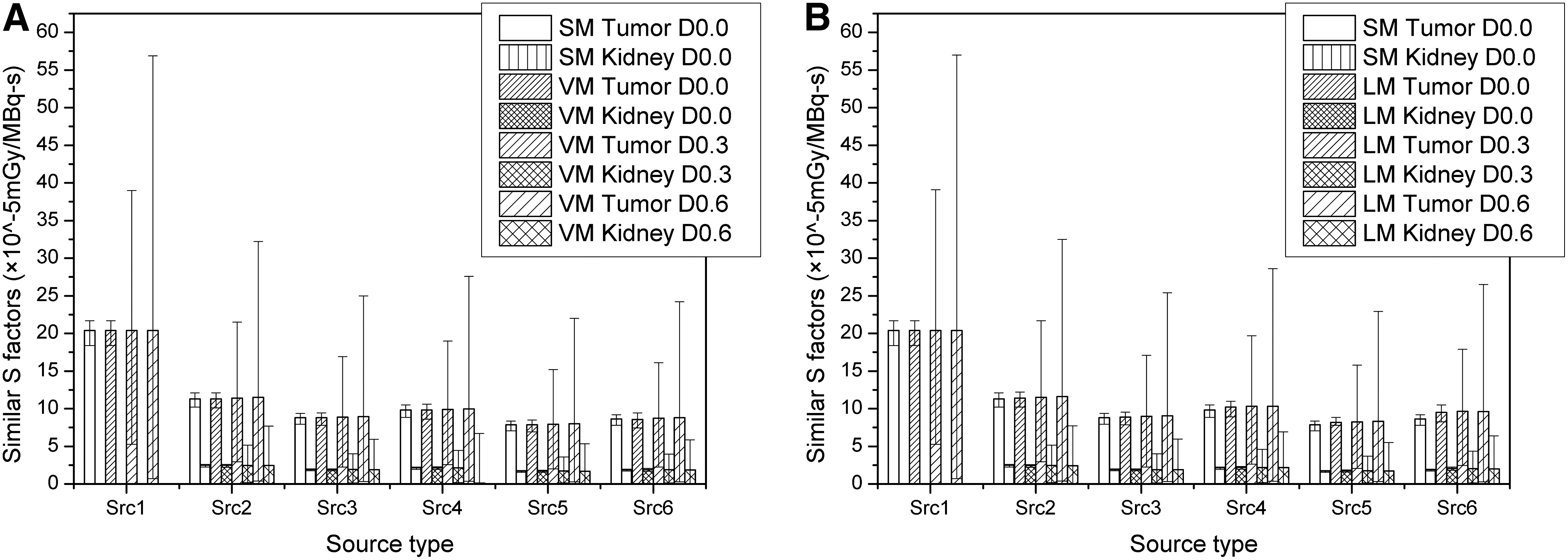
The mean, minimum, and maximum similar S factors (×10⁻⁵mGy/MBq-s) of the tumor and the kidney for multiple independent activity regions by (A) VM and SM methods; (B) LM and SM methods. Note: Src 1: tumor source; Src 2: tumor-kidney source; Src 3: tumor-kidney-spleen source; Src 4: tumor-kidney-liver source; Src 5: tumor-kidney-liver-spleen source; Src 6: tumor-kidney-liver-lung source.

Table 1 shows the initial injected total activity threshold in GBq. As far as the quasi-homogeneous activity distribution (D 0.0) is concerned, generally, the activity threshold suggested by the tumor is secure for the kidney protection. However, if the activity heterogeneous degree deteriorates, for example, D 0.3 and D 0.6, then the tolerant activity threshold of the kidney will be exceeded. Thus, as long as the kidney has activity and the activity distribution in the tumor is heterogeneous, either tumor clonogens survive to make TCP <37%, or the kidney suffers from radiation injury to make normal tissue complication probability (NTCP) >50%. One point should be noted, that is, although LM shows some un-consistence with VM, basically, the conclusion about the secure (i.e., prescription) dose limit considering the tumor and the kidney at the same time is similar.

Table 1.

The Minimal Response Initial Total Activity Threshold (in GBq) of the Tumor, and the Mean Tolerant Initial Total Activity Threshold of the Kidney

Source type	Sigma	0.0		0.3		0.6
	Organ	tumor	kidney	tumor	kidney	tumor	kidney
Src 1	VM, LM	0.33	—^a	1.14	—^a	8.66	—^a
Src 2	VM	0.59	1.12	2.03	1.14	15.0	1.15
	LM	0.59	1.13	2.04	1.15	15.0	1.15
Src 3	VM	0.77	1.45	2.67	1.46	19.4	1.47
	LM	0.76	1.46	2.67	1.47	18.8	1.48
Src 4	VM	0.70	1.30	2.34	1.31	17.4	1.32
	LM	0.67	1.27	2.29	1.28	17.0	1.30
Src 5	VM	0.87	1.63	2.99	1.64	20.7	1.65
	LM	0.77	1.59	2.91	1.60	20.0	1.62
Src 6	VM	0.81	1.47	2.68	1.49	22.6	1.50
	LM	0.73	1.35	2.46	1.37	20.8	1.39

The minimal response initial total activity threshold (in GBq) of the tumor is obtained by setting the minimal voxel dose of 60 Gy for the tumor, and the mean tolerant initial total activity threshold of the kidney is obtained by setting the averaged voxel dose of 28 Gy for the kidney.

For only the single β spectrum of ¹³¹I, not including the γ spectrum, used here, thus, actually the result is unreasonable, and is not shown here.

Src 1, tumor source; Src 2, tumor-kidney source; Src 3, tumor-kidney-spleen source; Src 4, tumor-kidney-liver source; Src 5, tumor-kidney-liver-spleen source; Src 6, tumor-kidney-liver-lung source.

VM, voxel-by-voxel activity sample algorithm; LM, level partition method.

Discussion

Patient-specific 3-D Monte–Carlo methods for radionuclide dosimetry have been extensively implemented.^1

–9 Most of these Monte–Carlo codes have dealt with the quasi-homogeneous activity distribution and assumed that the activity and the resulting dose are homogeneous at the organ or tumor scale. However, in practice, the target is not uniform due to the inhomogeneous expression/distribution of receptors/antigens and the nonuniform vascularization of the tumor tissue, as well as the activity metabolism. Thus, the heterogeneous activity distribution at the sub-organic level simulated by the Monte–Carlo method cannot be avoided in the accurate radionuclide dosimetry. The single organ or tumor averaged dose cannot be considered sufficient to represent the therapeutic efficacy for either the tumor response or the toxicity for the normal tissue injury as well.

The LM divides the heterogeneous activity distribution into several homogeneous levels and assumes each level is a uniform activity distribution.^4,7,12 Song et al.⁷ have divided the activity into 5, 10, or 20 equally sized activity bins on the 3-D lung activity map. The voxels belonging to the same bin on the activity map have been merged on the density map and assigned the same universe number in the MCNP4B input file. However, this simulation work shows that if the activity distribution involves more than two independent activity regions, then the artifacts brought up by the activity binning or leveling should be cautious. If the voxel numbers of these independent activity regions are similar (for example, less two to three times), then the artifacts could be acceptable. However, if their voxel numbers are different from each other for more than about 10 times, then the artifacts will remarkably affect their calculation result. According to the typical activity distribution from the real image (e.g., ref.¹), the activity is extensively distributed in the whole patient body. Even the rest of the body absorbs activity in a proportion of 0.04 if the tumor is assumed to absorb activity in a proportion of 1. One method of avoiding these artifacts is by nonequally dividing the heterogeneous activity distribution into homogeneous levels. However, the activity-extensive distribution in the body will make the LM inclined to attend to one thing and lose another. The VM samples the source particle location according to the activity spatial distribution, and imparts the source particle weight by the relative activity concentration of its origination voxel to realize the dose calculation of the heterogeneous activity distribution. This algorithm essentially regards each non-zero activity voxel as an independent voxel sub-source, and the sub-source weight is consistent with its relative activity, that is, its source emitter emitting probability. Thus, this algorithm effectively avoids the leveling/binning artifacts.

The full dose distribution at the voxel or cell scale for the tumor or the organ at risk is very critical for the accurate patient dose-response analyses, especially for the radiobiological evaluation such as TCP and NTCP.^21,22 The well-known Poisson definition of TCP shows that even one survival clonogen will decrease the TCP from 100% to 37% to negatively affect the therapeutic efficacy. If the activity in the tumor or organ scale is homogeneous, generally, the minimal response initial activity threshold of the tumor will not threaten the kidney protection. However, if the activity in the tumor or organ scale is slightly inhomogeneous (e.g., Gauss distribution with sigma of 0.3), then the activity will have to be increased by more than thrice to kill the last tumor clonogen or voxel. The response minimal initial total activity threshold needed by the tumor will exceed the maximal tolerant mean initial total activity threshold required by the kidney. Thus, the kidney toxicity has to be worried about a lot at the same time. With the activity heterogeneous grade deteriorating (e.g., Gauss distribution with sigma of 0.6), the minimal response initial total activity threshold of the tumor will have to be increased by 25 times. Thus, actually, there is always a relative proportion of the tumor clonogen surviving now, as the prescription activity in clinics dares not use the activity so high considering the protection of the kidney or other normal organs.

The MIRD approach¹⁵ is commonly used in clinics to estimate the radionuclide organ dose for its convenience. The calculated S factors of this VM EGSnrc algorithm also has compared with those of DPM and MIRDOSE^1,23 (see Table 2). MIRDOSE adopted the MIRD Committee's Reference Man phantom.²⁴ The DPM self-absorbed S values had been processed by mass weighting from Zubal phantom to Reference Man phantom, but its cross-absorbed S values had not been processed. Here, these self-absorbed S values are processed by mass weighting from Reference Man phantom to Zubal phantom again. However, the cross-absorbed S values are still based on Zubal phantom for DPM and Reference Man phantom for MIRDOSE. Generally, the self-absorbed S-value of EGSnrc with the single β spectrum is about 20% lower than those of DPM and MIRDOSE results. If the energy spectrum is changed to include the γ emission, the difference of the self-absorbed S-value will increase to 30%. Here, the β and γ emission spectra of radionuclide ¹³¹I are from Health Physics Society website [http://hps.org/publicinformation/radardecaydata.cfm]. DPM^1,23 has used the Lawrence Berkeley/Lund Nuclear Data (version 2.0, 1999). From the viewpoint of the cross-fire S value, the result including γ emission is more reasonable than those of the single β spectrum, and lower than DPM and MIRDOSE. Song et al.²⁵ have obtained the lower result by MCNP4B based on the full photon and electron spectra of ¹³¹I and ⁹⁰Y from the Lund/LBNL Nuclear Data. They found that the lung-to-lung self-absorbed doses for ¹³¹I and ⁹⁰Y were about 6.0% lower and 13.4% lower, respectively, than those obtained from the OLINDA software package.²⁶

Table 2.

Comparison of ¹³¹ I S-Values (mGy/MBq-s) from VM EGSnrc, DPM, and MIRDOSE

		S-values (mGy/MBq-s)
Organs		VM EGSnrc
Source	Target	γ/β/e-	Single β	DPM	MIRDOSE
Liver	Liver	1.36E-05	1.46E-05	2.07e-5	2.04e-5
Kidney	Kidney	4.81E-05	5.60E-05	6.95e-5	6.83e-5
Spleen	Spleen	6.66E-05	7.62E-05	9.68e-5	9.34e-5
Liver	Kidney	5.49E-07	1.87E-08	1.18e-6	8.13e-7
Liver	Spleen	1.37E-07	1.34E-12	2.71e-7	2.14e-7
Kidney	Liver	5.49E-07	1.85E-08	1.17e-6	8.13e-7
Kidney	Spleen	8.85E-07	3.29E-08	1.83e-6	1.85e-6
Spleen	Liver	1.38E-07	1.24E-11	2.72e-7	2.14e-7
Spleen	Kidney	8.86E-07	3.29E-08	1.83e-6	1.85e-6

The DPM and MIRDOSE data^1,23 have been processed by mass weighting from Reference Man phantom to Zubal phantom.

To verify our algorithm more, single and homogeneous organ sources for the mono-energic photon S factor and electron SAFs have been simulated and compared with some published MCNP/MCNPX work (see the Supplementary Data available online at www.liebertonline.com/cbr). Supplementary Tables S1–S4 show the organ SAF for 100 keV–1 MeV photon and S factor for 0.935 MeV electron for organ sources with the electron and photon cutoff kinetic energies of 1 keV, which are compared with published MCNP/MCNPX results as well as 1 keV cutoff energies.^4,6,9 Generally, the differences between them are <10%. Basically, EGSnrc SAF is between those of MCNP and MCNPX. As for the low energy electron similar to 0.935MeV, most of the energy is deposited in the source organ (Supplementary Table ST4). The cross-organ S factor is a lot lower. The self-absorbed or cross-fire S factors between the kidney and liver are basically consistent with those of MCNP/MCNPX. Thus, these differences of EGSnrc with MIRDOSE, DPM, and MCNP4B of ¹³¹I should be due to the effect of different energy spectra, transport algorithms, and cross-section data, as well as different phantoms. The simple mass weighting from one phantom organ to other phantom organ using a rough linear process also produces partial differences.

Conclusions

A VM is presented that calculates the dose of the heterogeneous activity distribution for the radionuclide dosimetry. This algorithm is applied to calculate the DVH for multiple independent activity regions with Gauss diffusion activity distributions, and then compared with the LM. The result shows that the new algorithm is more consistent with the weighted superposition of the quasi-homogeneous activity distribution than the LM, especially for the multiple independent activity regions composed of different amounts of voxels. The new algorithm effectively avoids the leveling/binning artifacts to the heterogeneous activity distribution.

Footnotes

Acknowledgments

The work is supported by the Chinese National Natural Science Foundation (10805012), Fundamental Research Funds for the Central Universities (2010HGXJ0216; 2012HGXJ0057), Seed Foundation of the Hefei University of Technology (2012HGZY0007), and Scientific Research Foundation for Returned Scholars, Ministry of Education of China.

Disclosure Statement

No competing financial interests exist.

References

Dewaraja

, Wilderman

, Ljungberg

et al. Accurate dosimetry in ¹³¹I radionuclide therapy using patient-specific, 3-dimensional methods for SPECT reconstruction and absorbed dose calculation. J Nucl Med, 2005; 46:840.

Furhang

, Chui

, Kolbert

et al. Implementation of Monte Carlo dosimetry method for patient-specific internal emitter therapy. Med Phys, 1997; 24:1163.

Liu

, Williams

, Lopatin

et al. A radionuclide therapy treatment planning and dose estimation system. J Nucl Med, 1999; 40:1151.

Yoriyaz

, Stabin

, dos Santos

. Monte Carlo MCNP-4B-based absorbed dose distribution estimates for patient-specific dosimetry. J Nucl Med, 2001; 42:662.

Ljungberg

, Sjogreen

, Liu

et al. A three dimensional absorbed dose calculation method based on quantitative SPECT for radionuclide therapy: Evaluation for I-131 using Monte Carlo simulation. J Nucl Med, 2002; 43:1101.

Chiavassa

, Aubineau

, Bitar

et al. Validation of a personalized dosimetric evaluation tool (Oedipe) for targeted radiotherapy based on the Monte Carlo MCNPX code. Phys Med Biol, 2006; 51:601.

Song

, He

, Prideaux

et al. Lung dosimetry for radioiodine treatment planning in the case of diffuse lung metastases. J Nucl Med, 2006; 47:1985.

Descalle

, Hartmann Siantar

, Dauffy

et al. Application of MINERVA Monte Carlo simulations to targeted radionuclide therapy. Cancer Biother Radiopharm, 2003; 18:71.

Chiavassa

, Bardiès

, Guiraud-Vitaux

et al. OEDIPE: A personalized dosimetric tool associating voxel-based models with MCNPX. Cancer Biother Radiopharm, 2005; 20:325.

10.

Hadid

, Desbrée

, Schlattl

et al. Application of the ICRP/ICRU reference computational phantoms to internal dosimetry: Calculation of specific absorbed fractions of energy for photons and electrons. Phys Med Biol, 2010; 55:3631.

11.

Neti

PVSV

, Howell

. Log normal distribution of cellular uptake of radioactivity: Implications for biologic responses to radiopharmaceuticals. J Nucl Med, 2006; 47:1049.

12.

Sgouros

, Squeri

, Ballangrud

et al. Patient-specific, 3-dimensional dosimetry in non-Hodgkin's lymphoma patients treated with 131I-anti-B1 antibody: Assessment of tumor dose-response. J Nucl Med, 2003; 44:260.

13.

Kawrakow

, Mainegra-Hing

, Rogers

DWO

et al. The EGSnrc Code System: Monte Carlo Simulation of Electron and Photon TransportNRCC Report PIRS-7012010.

14.

Prideaux

, Song

, Hobbs

et al. Three-dimensional radiobiologic dosimetry: application of radiobiologic modeling to patient-specific 3-dimensional imaging–based internal dosimetry. J Nucl Med, 2007; 48:1008.

15.

Loevinger

, Budinger

, Watson

. MIRD Primer for Absorbed Dose Calculation. New York: Society of Nuclear Medicine, 1988.

16.

Zubal

, Harrell

, Smith

et al. Computerized three-dimensional segmented human anatomy. Med Phys, 1994; 21:299.

17.

Stabin

, da Luz

LCQP

. Decay data for internal and external dose assessment. Health Phys, 2002; 83:471.

18.

Dale

. Use of the linear-quadratic radiobiological model for quantifying kidney response in targeted radiotherapy. Cancer Biother Radiopharm, 2004; 19:363.

19.

Sgouros

. Dosimetry of internal emitters. J Nucl Med, 2005; 46,1 suppl:18S.

20.

Emami

, Lyman

, Brown

et al. Tolerance of normal tissue to therapeutic irradiation. Int J Radiat Oncol Biol Phys, 1991; 21:109.

21.

Lin

, Jing

, Xu

. Effect of different cell-cluster models on the radiobiological output for 211At-radioimmunotherapy. Cancer Biother Radiopharm, 2011; 26:85.

22.

Lin

, Jing

, Xu

et al. Combining NTCP LKB model with radiosensitivity parameters to characterize toxicity of radionuclides based on a multi-clonogen kidney model: a theoretical assessment. Australas Phys Eng Sci Med, 2012, DOI:10.1007/s13246-012-0141-5.

23.

Wilderman

, Gunnett

, Kearfott

et al. Fast CT/SPECT derived 3D Monte Carlo dose computations for I-131 internal emitter therapy. Conference Record: IEEE Nuclear Science Symposium and Medical Imaging Conference, Rome, Italy, October 16–22, 2004.

24.

Stabin

. MIRDOSE: Personal computer software for internal dose assessment in nuclear medicine. J Nucl Med, 1996; 37:538.

25.

Song

, Du

, Sgouros

et al. Therapeutic potential of 90Y- and 131I-labeled anti-cd20 monoclonal antibody in treating non-hodgkin's lymphoma with pulmonary involvement: A Monte Carlo–based dosimetric analysis. J Nucl Med, 2007; 48:150.

26.

Stabin

, Sparks

, Crowe

. OLINDA/EXM: The second-generation personal computer software for internal dose assessment in nuclear medicine. J Nucl Med, 2005; 46:1023.

Supplementary Material

Please find the following supplemental material available below.

For Open Access articles published under a Creative Commons License, all supplemental material carries the same license as the article it is associated with.

For non-Open Access articles published, all supplemental material carries a non-exclusive license, and permission requests for re-use of supplemental material or any part of supplemental material shall be sent directly to the copyright owner as specified in the copyright notice associated with the article.

0.00 MB

0.04 MB