Evaluating the Application of Tissue-Specific Dose Kernels Instead of Water Dose Kernels in Internal Dosimetry: A Monte Carlo Study

Abstract

Purpose:

The aim of this work is to evaluate the application of tissue-specific dose kernels instead of water dose kernels to improve the accuracy of patient-specific dosimetry by taking tissue heterogeneities into consideration.

Materials and Methods:

Tissue-specific dose point kernels (DPKs) and dose voxel kernels (DVKs) for yttrium-90 (⁹⁰Y), lutetium-177 (¹⁷⁷Lu), and phosphorus-32 (³²P) are calculated using the Monte Carlo (MC) simulation code GATE (version 7). The calculated DPKs for bone, lung, adipose, breast, heart, intestine, kidney, liver, and spleen are compared with those of water. The dose distribution in normal and tumorous tissues in lung, liver, and bone of a Zubal phantom is calculated using tissue-specific DVKs instead of those of water in conventional methods. For a tumor defined in a heterogeneous region in the Zubal phantom, the absorbed dose is calculated using a proposed algorithm, taking tissue heterogeneity into account. The algorithm is validated against full MC simulations.

Results:

The simulation results indicate that the highest differences between water and other tissue DPKs occur in bone for ⁹⁰Y (12.2% ± 0.6%), ³²P (18.8% ± 1.3%), and ¹⁷⁷Lu (16.9% ± 1.3%). The second highest discrepancy corresponds to the lung for ⁹⁰Y (6.3% ± 0.2%), ³²P (8.9% ± 0.4%), and ¹⁷⁷Lu (7.7% ± 0.3%). For ⁹⁰Y, the mean absorbed dose in tumorous and normal tissues is calculated using tissue-specific DVKs in lung, liver, and bone. The results are compared with doses calculated considering the Zubal phantom water equivalent and the relative differences are 4.50%, 0.73%, and 12.23%, respectively. For the tumor in the heterogeneous region of the Zubal phantom that includes lung, liver, and bone, the relative difference between mean calculated dose in tumorous and normal tissues based on the proposed algorithm and the values obtained from full MC dosimetry is 5.18%.

Conclusions:

A novel technique is proposed considering tissue-specific dose kernels in the dose calculation algorithm. This algorithm potentially enables patient-specific dosimetry and improves estimation of the average absorbed dose of ⁹⁰Y in a tumor located in lung, bone, and soft tissue interface by 6.98% compared with the conventional methods.

Introduction

The spatial distribution of radiotracers used in internal radionuclide therapy is not uniform and, therefore, three-dimensional (3D), patient-specific dosimetry has become an important research topic.¹ Although accurate patient-specific dosimetry is not commonly performed in clinical practice.²

The advent of single-photon-emission computed tomography (SPECT) and positron emission tomography (PET) scanners coupled with X-ray computed tomography (CT) can be used to derive a more individualized dose distribution. The first step to calculate the absorbed dose is to estimate the tracer's activity distribution^3,4 using SPECT/CT or PET/CT imaging techniques.^5
–7 To calculate dose distribution from the activity map, two common approaches are available: full Monte Carlo (MC) simulation and analytic calculation. Despite the fact that hardware and software have been improved substantially, the application of full MC dosimetry using patient characteristics in clinical practice is still time consuming.⁸ As such, analytic techniques to speed up the calculation process are preferred. One of these analytic methods is convolving MC-generated dose point kernels (DPKs) or dose voxel kernels (DVKs) with the activity distribution (or activity map) at the voxel level.⁹

More than four decades ago, Loevinger et al.¹⁰ introduced the concept of “Point Source Dose Functions” for β particle emitting radionuclides. After providing the solution to the electron transport equation by Spencer,¹¹ Berger¹² was the first who implemented an MC method to simulate electron transport. The concept of electron point kernel for β particle dosimetry was first introduced by Berger in 1973.¹³ DPKs are calculated by simulating radiation transports across a homogeneous medium, using MC code. The absorbed dose at predefined distances is regarded as DPKs.¹⁴ DVKs are defined based on the dose distribution in a Cartesian dose scoring grid that is located around a uniform voxel source or a source located in the center of the voxel.¹⁵

To calculate β particle DPKs, different MC codes such as PENELOPE, GEANT4, MCNPX, FLUKA, and ETRAN have been suggested.^16,17 This study is performed using GATE (version 7),¹⁸ a validated MC simulation code for tomographic emission and recently radiotherapy applications. Electron DPKs in GATE were validated by Maigne et al.¹⁹ for an energy range between 15 keV and 20 MeV. This code was also validated in nuclear medicine by Papadimitroulas et al.⁸

In this study, tissue-specific DPKs for ⁹⁰Y, ¹⁷⁷Lu, and ³²P are computed and compared with those of water. The results demonstrate that although the differences between water and soft tissue DPKs are negligible, lung and bone DPKs are significantly different from those of water. As such, patient-specific dosimetry requires a combination of tissue-specific dose kernels and anatomic data along with modified algorithms. To the best of our knowledge, clinical radionuclide dosimetry approaches generally ignore tissue heterogeneity and the human body is assumed water equivalent.^20

–23

In this study, various tumors located in bone, lung, and liver of a Zubal phantom²⁴ are defined and the dose distribution in tumorous and normal tissues is calculated using the corresponding dose kernels. The obtained results are compared with those obtained by water-equivalent Zubal phantom to assess the impact of using patient-specific dose kernels in calculation algorithms.

To decrease the computation time of the convolution algorithm, Fast Fourier Transform (FFT) or Fast Hartley Transform is used rather than direct convolution.²⁵ In convolution algorithm based on FFT, a constant dose kernel should be used, which leads to the inevitable assumption of a homogeneous medium in the dose calculation algorithm. Reported differences as a result of material variations indicate that this assumption is not accurate^8,26 and more precise dose calculation algorithms should be used.

One of the earliest methods to take tissue heterogeneity into consideration was path length modification. In this approach, various rescaling methods have been used.^27
–29 Loudos et al.³⁰ used kernel data to derive a material-dependent dose absorption factor in each voxel. In this method, dose distribution was calculated using water-based dose kernels and then for each voxel a correction factor was applied. A density correction factor for each voxel in the abdominal region for soft tissues was introduced by Dieudonne et al.²⁰ In this technique, the correction factor for each voxel was the ratio of water density to the density of the voxel material. Although this technique improved the results in the abdominal region, the application of this method in highly heterogeneous regions requires more research. In another method, Sanchez-Garcia et al.³¹ scaled DPKs based on the radiological interval between the source point and energy deposition sites. In this technique, it is not feasible to use the convolution algorithm. As such, the impacts of all source points on target locations were superimposed based on the collapsed cone principle to calculate the absorbed dose.³¹

In the foregoing studies, various correction factors were introduced to take tissue heterogeneity into account and improve the accuracy of estimating dose distribution. It must be noted that in all these methods, the absorbed doses have been measured using water dose kernels and then the correction factors were applied to the results. However, we try to apply organ-specific dose kernels and the corresponding correction factor for each voxel during the calculation process based on a proposed dose calculation algorithm to improve dose estimation accuracy compared with the conventional methods. In this technique, the correction factors were extracted from material-specific DVKs. The validation of the proposed algorithm was performed on a tumor defined in a heterogeneous region of the Zubal phantom against direct MC simulations for ⁹⁰Y.

The main goals of this study are summarized as follows: first to quantify the impact of using tissue-specific dose kernels instead of those of water in a dose-calculation algorithm applied to the Zubal phantom, second to present a new algorithm to improve the accuracy of dose distribution estimation taking tissue heterogeneities into account, thus enabling accurate patient-specific dosimetry, and finally to validate the proposed algorithm against full MC simulation as the reference standard.

Materials and Methods

Calculation of DPKs

Simulation parameters

DPKs are calculated using the MC simulation code GATE (version 7),¹⁸ an upper layer of Geant4 using Geant4.9.6 cross section libraries. DPKs are calculated in a spherical phantom composed of various tissue materials. A point source with isotropic emission is simulated at the center of the sphere. It should be guaranteed that all the emitted particles deposit their entire energy inside the sphere. For this purpose, GATE visualization tool is used to select the sphere size; in some cases the spheres should be simulated slightly bigger than the electron ranges emitted as β particles.

In GATE, materials can be described precisely by providing their density, elements' atomic number, and their composition.^32,33 In this study, adipose, bone, breast, heart, intestine, kidney, liver, lung, and spleen tissues are considered for DPK calculation. Among available sources in radionuclide therapy, β particle emitting radionuclides are the most prevalent options. Hence, in this study, DPKs are generated for three commonly used radionuclides in nuclear medicine, including ⁹⁰Y, ¹⁷⁷Lu, and ³²P.

In the current simulation, Geant4.9.6 “Standard” model is used for the physical processes except for the Rayleigh process in which the Penelope model is used. In this model, the energy range of photon and electron interactions is 1 keV to 100 TeV, which covers the energy range 1 keV to a few MeV in our simulation. Bremsstrahlung, electron ionization, and electron multiple scattering are the physical interactions included in the simulation. Each radionuclide energy spectrum is taken from the study of Prestwich et al.¹⁴ For ¹⁷⁷Lu, the small contribution of γ emission to the absorbed dose is neglected and only β particle dose kernels are calculated for this radionuclide.

The “stepHitType” parameter in GATE is used to adjust the energy deposition site. The energy of the hits in this study is deposited randomly along the electron step to decrease the calculation uncertainty. GATE also suggests that the number of table bins for mass stopping power “dE/dX binning” and mean free path “Lambda binning” should be set equal to 220.

The calculated absorbed doses are stored in a 3D matrix and the voxel values at the same distance from the point source are added. This summation composes concentric shells around the point source. The thickness of these voxelized shells is determined based on the size of the matrix voxel. As at least one interaction in each voxel is desirable, the voxel size is defined equal to the “electronStepLimiter,”¹⁷ which limits the maximum size of electron steps in simulation.³⁴

In GATE, each particle track is composed of many steps. The Bethe–Bloch formula³⁵ is used to calculate ionization energy loss along each step, because of Bremsstrahlung emission and secondary electron production. For assuming a constant interaction cross section along the step, the step size should be as small as possible. In addition, generated secondary electrons are tracked throughout each step, provided that particle energy exceeds production threshold. In GATE, this threshold is indicated in a range rather than energy to be independent of particle type and medium. Selection of a smaller production threshold increases the number of secondary electrons, which leads to a more accurate simulation but longer computation time. To accurately simulate the nonlinearity of electron tracks and improve the accuracy of generated DPKs, the electronStepLimiter should be as small as possible. In contrast, the smaller the electronStepLimiter, the longer the simulation time. In this study, the electronStepLimiters are determined in such a way that the achieved results are consistent with the published results in the study of Papadimitroulas et al.⁸ This method is an empirical technique and more research is required to determine the electronStepLimiter more accurately, which is beyond the scope of this study. The simulation parameters in water are presented in Table 1.

Table 1.

Parameters of Monte Carlo Simulation in Water

Isotope	Sphere radius in water (mm)	ElectronStepLimiter in water (mm)	Number of shells	Number of assessed voxels
Yittrium-90	11	1.1 × 10⁻¹	100	23
Phosphorus-32	7.59	0.690 × 10⁻¹	110	28
Lutetium-177	3	1.504 × 10⁻²	200	43

The sphere radius and the magnitude of the electronStepLimiter determine the number of the concentric shells around the point source for each radionuclide. Accordingly, the number of shells for the mentioned radionuclides is not identical and about 100–200 spherical shells are specified in each simulation.¹⁷ Furthermore, the mean range of the β particles for each radionuclide with the corresponding electronStepLimiter defines the number of assessed voxels in the simulation. ¹⁷⁷Lu has significantly smaller electronStepLimiter than ⁹⁰Y and ³²P; accordingly, it is associated with larger number of the shells and assessed voxels.

To validate our simulations, the calculated DPK profiles in water are compared with the published results of Papadimitroulas et al.⁸ for ⁹⁰Y and ¹⁷⁷Lu. The comparison of the two profiles is performed at identical distances from the source. After validating simulated water DPKs, tissue-specific DPKs in bone, lung, adipose, breast, heart, intestine, kidney, liver, and spleen are calculated and compared with those of water according to Equation (1). \documentclass{aastex}\usepackage{amsbsy}\usepackage{amsfonts}\usepackage{amssymb}\usepackage{bm}\usepackage{mathrsfs}\usepackage{pifont}\usepackage{stmaryrd}\usepackage{textcomp}\usepackage{portland, xspace}\usepackage{amsmath, amsxtra}\pagestyle{empty}\DeclareMathSizes{10}{9}{7}{6}\begin{document} \begin{align*}{ \frac { \left\vert { { D_ { w } } \left( r \right) - { D_ { t} } \left( r \right) } \right\vert } { { \rm { max } } \left( { { D_ { w } } , { D_ { t } } } \right) } } \times 100 \% \quad \quad \quad { \rm Eq. } \ ( 1 ) \end{align*} \end{document}

In this equation, D_w (r) is the absorbed dose in water at distance r from the point source and D_t (r) is the absorbed dose in tissue at the same distance, as a percentage of the maximum value of the two calculated absorbed doses.

To display DPK profiles, Cross et al.³⁶ suggested dimensionless axes according to Equation (2). The calculated water DPK for ⁹⁰Y is illustrated in Figure 1. The y-axis represents the scaled absorbed dose and is defined as \documentclass{aastex}\usepackage{amsbsy}\usepackage{amsfonts}\usepackage{amssymb}\usepackage{bm}\usepackage{mathrsfs}\usepackage{pifont}\usepackage{stmaryrd}\usepackage{textcomp}\usepackage{portland, xspace}\usepackage{amsmath, amsxtra}\pagestyle{empty}\DeclareMathSizes{10}{9}{7}{6}\begin{document} \begin{align*} J \left( {r / {X_{90}}} \right) = 4 \ \pi {r^2}D \left( {r , E} \right) {X_{90}} / \overline E , \quad \quad \quad { \rm Eq.} \ ( 2 ) \end{align*} \end{document}

FIG. 1.

⁹⁰Y water DPK. DPK, dose point kernel.

where r is the radial distance from the point source and D (r, E) is the absorbed dose per particle at distance r. In this equation, Ē indicates the average energy of the isotope's β particle energy spectrum and X ₉₀ represents the radius of a sphere in which 90% of the β particle energy is deposited.³⁷ X ₉₀, which depends on the radionuclide average energy and the source medium, was defined in the study of Botta³⁸ for ¹⁷⁷Lu and ⁹⁰Y and in that of Mainegra-Hing et al.³⁹ for ³²P in water. The mentioned parameters for each isotope are shown in Table 2.

Table 2.

The Parameters of β Particle Emitting Radionuclides

Isotope	X ₉₀ in water (mm)	Maximum β particle energy (MeV)	Average energy of β particle spectrum (keV)	Mean range of β particles in water (mm)	Maximum range of β particles in water (mm)
Yttrium-90	5.40	2.27	935.3	2.5	11
Phosphorus-32	3.66	1.709	696.3	1.98	7.6
Lutetium-177	0.62	0.497	133.5	0.67	2.2

The number of simulated particles is selected equal to 2 × 10⁸ for ⁹⁰Y and 2 × 10⁹ for ³²P and ¹⁷⁷Lu. In general, the number of initially emitted particles is simulated in such a way to keep the associated statistical uncertainty less than 5% at each point along the mean range of β particles.⁴⁰ The total dose statistical uncertainty is kept less than 2.0% along the mean range of β particles. The simulation uncertainties for ⁹⁰Y, ³²P, and ¹⁷⁷Lu DPKs in water are illustrated in Table 3.

Table 3.

Dose Point Kernels Simulation Uncertainty for ⁹⁰ Y, ³² P, and ¹⁷⁷ Lu in Water

⁹⁰Y		³²P		¹⁷⁷Lu
Distance (mm)	Uncertainty (%)	Distance (mm)	Uncertainty (%)	Distance (mm)	Uncertainty (%)
0.11	0.21	0.07	0.058	0.015	0.02
0.22	0.17	0.21	0.059	0.045	0.36
0.33	0.22	0.35	0.14	0.075	0.98
0.44	0.32	0.42	0.24	0.09	1.14
0.55	0.45	0.56	0.36	0.12	1.86
0.66	0.61	0.7	0.61	0.16	1.71
0.77	0.78	1.05	0.93	0.21	1.59
0.88	0.99	1.19	1.03	0.27	1.99
0.99	1.2	1.33	1.14	0.33	2.1
1.1	1.43	1.4	1.23	0.36	2.6
1.21	1.69	1.54	1.3	0.4	3.11
1.32	1.97	1.61	1.4	0.45	3.37
1.43	2.2	1.75	1.5	0.51	3.53
1.54	2.48	1.89	1.62	0.55	3.88
1.65	2.8	1.96	1.75	0.6	4.19
1.76	3.06	2.1	1.89	0.66	5.3
1.87	3.33	2.24	2.1	0.72	8.4
1.98	3.69	2.38	2.24	0.76	20.14
2.09	3.95	2.45	2.37	—	—
2.2	4.3	—	—	—	—
2.31	4.73	—	—	—	—
2.42	4.99	—	—	—	—
2.53	5.3	—	—	—	—

Tissue-specific DPKs are calculated and compared with those of water at identical distances from the point source. The measured lung and bone DPKs are considerably different from those of the water. Accordingly, the impact of using tissue-specific DPKs instead of the water DPKs in the dose calculation algorithm for bone, lung, and soft tissue is quantified in the next section.

Dose calculation algorithm in homogeneous medium

To further assess the utilization of tissue-specific dose kernels rather than those of water, ⁹⁰Y dose distribution in a Zubal phantom²⁴ is calculated for defined tumors located in lung, liver, and bone. The adult Zubal phantom has 56 segmented organs and is composed of a 128 × 128 × 243 array of 4 × 4 × 4 mm³ voxels. The shape and location of organs are simulated based on CT images.

The β particle range of ⁹⁰Y is 11 mm in water and is less in bone. As a result, ⁹⁰Y β particles travel up to three voxels in all directions in the Zubal phantom in bone and soft tissue. As long as the tumors are located three voxels away from soft tissue and bone boundaries, and the activity is simulated inside the specified organs, we can guarantee that β particles emitted by ⁹⁰Y deposit all their energy in the designated organs, so tissue-specific dose kernels can be used in the convolution algorithm. For this purpose, we added tumors with the mentioned characteristic to liver and bone sites in the Zubal phantom using MATLAB. In contrast, in lung, the lower density (about 0.26 g/cc) allows longer β particle penetration, which increases the range of β particles up to 44 mm.²² Accordingly, β particles can travel up to 12 voxels in the lung of the Zubal phantom. In this respect, the lung tumor is defined 12 voxels away from the boundaries. Transverse slices of the Zubal phantom with tumors are shown in Figure 2a–c.

FIG. 2.

Representative slices through the anthropomorphic Zubal phantom showing a tumor defined with MATLAB in: (a) liver, (b) lung, (c) bone, and (d) lung, bone, and soft tissue boundaries.

Tissue-specific DVKs are convolved with activity assigned to each voxel in the phantom to calculate the absorbed dose distribution in each organ of interest. DVKs for water, lung, and bone are calculated using GATE (version 7) and electron transports are simulated in a Cartesian geometry and the energy deposition is scored in each element of a voxelized array surrounding a voxel in which the source is located in its center. Dimensions of each voxel are selected as 4 × 4 × 4 mm³, equal to the voxel size of the Zubal phantom. As was mentioned, ⁹⁰Y β particles travel up to three voxels in all directions in bone and soft tissue of the Zubal phantom. If we assume the source point at the center of the source voxel in the designated tissues, DVK matrix size should be 5 × 5 × 5 to cover the range of ⁹⁰Y β particles in bone and soft tissue isotropically. For lung, the defined DVK matrix size is 20 × 20 × 20.

To define activity map in our simulation, an activity of 10 Bq is assigned to each voxel for normal liver, lung, and bone regions as background activity, 80 Bq and 90 Bq are assigned to tumor peripheral voxels, and 100 Bq is assigned to the central voxels of the tumor in the Zubal phantom.^41,42 The spatial convolution of this activity map with the corresponding DVK yields 3D organ absorbed dose. The voxel size of DVK and the resulting dose map are equal to the voxel size of the Zubal phantom (i.e., 4 × 4 × 4 mm³).

To assess the impact of tissue-specific dose kernel application on tumorous and normal absorbed dose, two approaches for dose calculation are compared. First, the activity map is convolved with water DVK based on Fourier transform. Accordingly, normal and tumorous tissues are considered water equivalent. Second, the tissue-specific DVK is considered in the dose calculation algorithm for each organ (lung DVK for lung tissue, liver DVK for liver tissue, and bone DVK for bone tissue)

Dose calculation algorithm in heterogeneous medium

In this study, a dose calculation algorithm is introduced that takes tissue heterogeneity into consideration to improve the accuracy in patient-specific dosimetry. To assess the new algorithm, we define a tumor in the Zubal phantom at an interface among soft tissue, bone, and lung tissues in such a way to include the boundaries of the mentioned organs, using MATLAB. A slice of the Zubal phantom demonstrating this tumor is shown in Figure 2d.

For the first step, the Zubal phantom is divided into four segments, including air, bone, soft tissue, and interface regions. This tissue segmentation is performed based on tissue density information. A 5 × 5 × 5 kernel in which each voxel side is 4 mm isotropically covers ⁹⁰Y β particle ranges in bone and soft tissues, when the source is located at the center of the kernel. In contrast, because of the longer range of ⁹⁰Y β particles in lung, a 20 × 20 × 20 kernel is used. If all the surrounding voxels are identical, the index of the central voxel is saved in a new matrix with the name of the corresponding organ. As such, bone, lung, and soft tissue organs are segmented and the corresponding matrices with the same size as dose matrix are generated. These matrices have nonzero matrix elements in organ regions, whereas the organ voxels are at least 3 voxels away from the bone and soft tissues boundaries and at least 10 voxels away from the lung boundaries. In these three matrices, all the voxels located between the source and target voxel are identical. The absorbed dose in these organs can be calculated by convolving tissue-specific DVKs with the designated activity map based on the Fourier transform.

In contrast, if the voxels surrounding the source voxel are not identical, the central voxel is saved in a new matrix called interface. The size of this matrix is the same as the dose matrix and the values of the matrix elements are not 0 at lung–soft tissue, bone–soft tissue, and lung–bone boundaries. In Figure 3a, a schematic example of interface regions in lung–soft tissue and bone–soft tissue boundaries is illustrated. If the source voxel is located in the bone–soft tissue boundary, β particles could travel at most three voxels away from the source voxel isotropically. As such to perform the segmentation, the bone–soft tissue interface region is defined in such a way to encompass three voxels in each side of the bone–soft tissue boundary. In contrast, as the range of β particles of ⁹⁰Y in the lung of Zubal phantom is 11 voxels, 11 voxels should be considered to determine the lung–soft tissue interface. A transverse slice of the interface matrix in the Zubal phantom is demonstrated in Figure 3b.

FIG. 3.

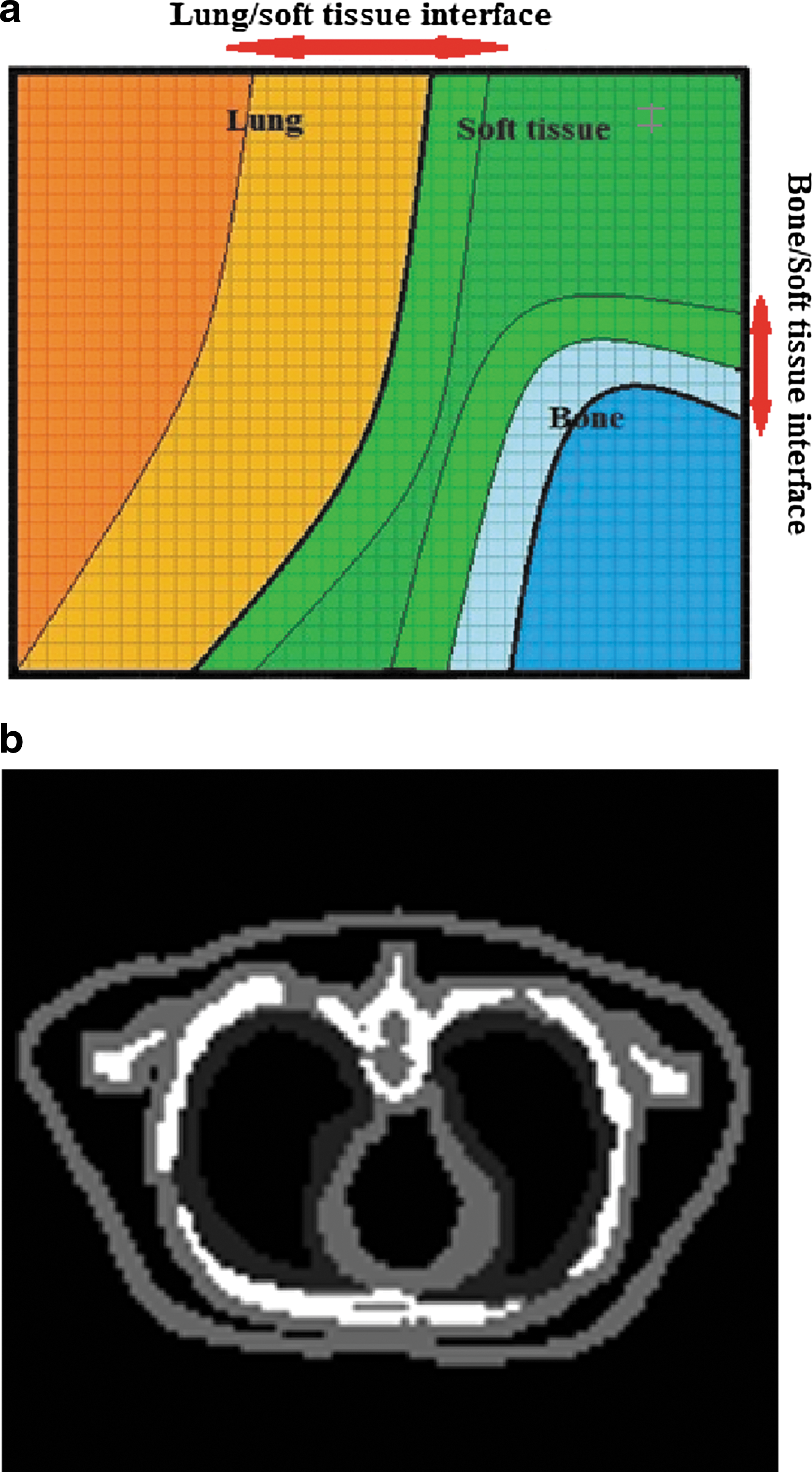
Lung, bone, soft tissue, and interface segmented regions in (a) a schematic example and (b) a transverse slice of the Zubal phantom. Color images available online at www.liebertpub.com/cbr

In the next step, to calculate the absorbed dose in the interface region, it is not feasible to convolve activity map with soft tissue, lung, and bone DVKs at the same time.³⁰ Therefore, we proposed a new superimposition algorithm for dose calculation in this region. At first, we specify the voxels located in the interface region that irradiate the surrounding voxels. Thereafter, the impact of these voxels on the surrounding target voxels is calculated. In this regard, DVKs are 5 × 5 × 5 kernels for bone and soft tissue and a 10 × 10 × 10 kernel for lung. Accordingly, if the location of the source voxel is considered to be in the center of these kernels that is assigned to (0, 0, 0), DVK (0, 0, 0) would be the self-irradiation factor of the source voxel. To assess the impact of the source voxel on the surrounding voxels, the location of the target voxels relative to source voxel is specified with i, j, and k indexes. Although the kernel shifts, the center of the kernel is located on top of the source voxel and the target voxels are the surrounding elements that are indexed from −2 to 2 for bone and soft tissue and from −10 to 10 for lung. As such, two sets are assigned to (i, j, k) for bone and soft tissue (set A) and lung (set B). \documentclass{aastex}\usepackage{amsbsy}\usepackage{amsfonts}\usepackage{amssymb}\usepackage{bm}\usepackage{mathrsfs}\usepackage{pifont}\usepackage{stmaryrd}\usepackage{textcomp}\usepackage{portland, xspace}\usepackage{amsmath, amsxtra}\pagestyle{empty}\DeclareMathSizes{10}{9}{7}{6}\begin{document} \begin{align*}& { \rm A} = \{ i , \ j , \ k \ \epsilon \,( - 2 , \ - 1 , \ 0 , \ 1 , \ 2 ) \} \\ & { \rm B} = \{ i , \ j , \ k \ \epsilon \,( - 10 , \ - 9 \ldots .0 \ldots 9 , \ 10 ) \} . \end{align*} \end{document}

To take tissue heterogeneity into consideration, anatomical information is used to specify the material in each voxel. In the interface region, there can be voxels of various materials between target and source voxels. To calculate dose distribution within this selected volume of interest, the intensity and the material of each voxel are determined. The voxel intensity indicates the amount of the activity in each voxel.

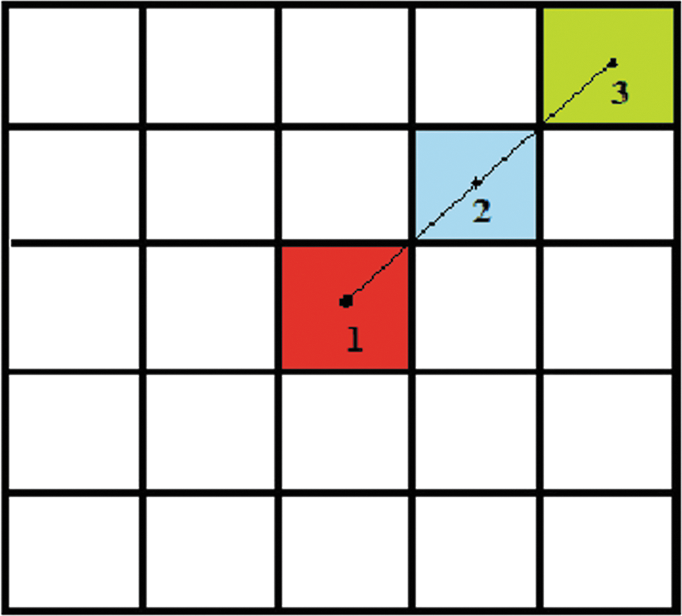
To assess the impact of the source voxel on the surrounding voxels, hypothetical lines between the centers of the source and target voxels are virtually drawn to determine the material of the voxels located between target and source voxels as well as the distance between them.

Tissue-specific dose kernels give the absorbed dose of the source voxel as a function of the distance from the source, as long as the emitted particles travel in the same corresponding tissue. For each voxel, a modification factor is calculated based on the obtained tissue-specific dose kernel values among two successive voxels according to Equation (3). This modification factor accounts for the material and location of the target voxels relative to the source voxel position and provides the amount of dose reduction when particles pass through this voxel. This factor is calculated based on the following equation. \documentclass{aastex}\usepackage{amsbsy}\usepackage{amsfonts}\usepackage{amssymb}\usepackage{bm}\usepackage{mathrsfs}\usepackage{pifont}\usepackage{stmaryrd}\usepackage{textcomp}\usepackage{portland, xspace}\usepackage{amsmath, amsxtra}\pagestyle{empty}\DeclareMathSizes{10}{9}{7}{6}\begin{document} \begin{align*} F \left( { i , j , k } \right) = { \frac { { \rm { DV } } { { \rm{ K } } _ { { \rm { target } } } } \left( { { \rm { i } } , \ { \rm { j } } , \ { \rm { k } } } \right) } { { \rm { DV } } { { \rm { K } } _ { { \rm { target } } } } \ \left( { I , \ J , \ K } \right) } } , \quad \quad \quad { \rm Eq. } \ ( 3 ) \end{align*} \end{document}

where (i, j, k) corresponds to the location of the target voxel and (I, J, K) defines the location of the voxel located on the aforementioned hypothetical line, just behind the target voxel, called from now on “previous voxel” as shown in Figure 4. The absorbed dose in the source voxel equals the product of the activity (intensity of the source voxel) by the tissue-specific DVK (0, 0, 0). The absorbed dose in each neighbor voxel is calculated based on the multiplication of the absorbed dose in the source voxel with the corresponding modification factor. This procedure is continued for the remaining target voxels located along the range of the emitted β particles. As such, regardless of the amount of the absorbed dose in the previous voxel, the modification factor determines the average of dose reduction in the target voxel. As a result, the absorbed dose for the target voxels in the interface region is calculated based on Equation (4). \documentclass{aastex}\usepackage{amsbsy}\usepackage{amsfonts}\usepackage{amssymb}\usepackage{bm}\usepackage{mathrsfs}\usepackage{pifont}\usepackage{stmaryrd}\usepackage{textcomp}\usepackage{portland, xspace}\usepackage{amsmath, amsxtra}\pagestyle{empty}\DeclareMathSizes{10}{9}{7}{6}\begin{document} \begin{align*}{D_{{ \rm{target \ voxel}}}} \left( {{ \rm{i}},{ \rm{j}},{ \rm{k}}} \right) = D \left( {I , \ J , \ K} \right) \times F \left( {i , j , k} \right), \quad \quad \quad { \rm Eq.} \ ( 4 ) \end{align*} \end{document}

where \documentclass{aastex}\usepackage{amsbsy}\usepackage{amsfonts}\usepackage{amssymb}\usepackage{bm}\usepackage{mathrsfs}\usepackage{pifont}\usepackage{stmaryrd}\usepackage{textcomp}\usepackage{portland, xspace}\usepackage{amsmath, amsxtra}\pagestyle{empty}\DeclareMathSizes{10}{9}{7}{6}\begin{document}$${D_{{ \rm{target \ voxel}}}} \left( {i , j , k} \right)$$ \end{document} is the absorbed dose in \documentclass{aastex}\usepackage{amsbsy}\usepackage{amsfonts}\usepackage{amssymb}\usepackage{bm}\usepackage{mathrsfs}\usepackage{pifont}\usepackage{stmaryrd}\usepackage{textcomp}\usepackage{portland, xspace}\usepackage{amsmath, amsxtra}\pagestyle{empty}\DeclareMathSizes{10}{9}{7}{6}\begin{document}$$\left( {i , j , k} \right)$$ \end{document} , from the source located in \documentclass{aastex}\usepackage{amsbsy}\usepackage{amsfonts}\usepackage{amssymb}\usepackage{bm}\usepackage{mathrsfs}\usepackage{pifont}\usepackage{stmaryrd}\usepackage{textcomp}\usepackage{portland, xspace}\usepackage{amsmath, amsxtra}\pagestyle{empty}\DeclareMathSizes{10}{9}{7}{6}\begin{document}$$\left( {0 , \ 0 , \ 0} \right)$$ \end{document} . This calculation is repeated for each source voxel irradiating target voxels in the interface region, and all the target voxels surrounding the corresponding source voxel. The total absorbed dose in each voxel in the interface region is finally obtained from summation of all partial doses from all source voxels.

The following is an example of the application of this algorithm.

Figure 4 shows a schematic example of three different voxels in the interface region. In this example, voxel 1 is the source voxel and irradiating the surrounding voxels, including voxels 2 and 3. The absorbed dose in voxel 1 is achieved from multiplication of the amount of activity in this voxel by DVK₁ (0, 0, 0) as shown in Equation (5) (the modification factor is 1). The index of DVK corresponds to voxel composition (i.e., DVK₁ corresponds to the voxel based on the tissue of voxel 1 in Fig. 4) \documentclass{aastex}\usepackage{amsbsy}\usepackage{amsfonts}\usepackage{amssymb}\usepackage{bm}\usepackage{mathrsfs}\usepackage{pifont}\usepackage{stmaryrd}\usepackage{textcomp}\usepackage{portland, xspace}\usepackage{amsmath, amsxtra}\pagestyle{empty}\DeclareMathSizes{10}{9}{7}{6}\begin{document} \begin{align*}{ \rm{Absorbed \ dose }} \ \left( {0 , \ 0 , \ 0} \right) = & { \rm{Activity }} \ \left( {0 , \ 0 , \ 0} \right) \\ & \times { \rm{DV}}{{ \rm{K}}_1} \ \left( {0 , \ 0 , \ 0} \right), \quad \quad \quad { \rm Eq.} \ ( 5 ) \end{align*} \end{document}

FIG. 4.

A schematic example of three various voxels in the interface region. In this example, voxel 1 contains activity and irradiating the surrounding voxels (2 and 3). Color images available online at www.liebertpub.com/cbr

where Activity (0, 0, 0) is the amount of activity in the source voxel and DVK₁ (0, 0, 0) is the source DVK in (0, 0, 0). To calculate the absorbed dose in the surrounding voxels (indicated by 2 and 3 in Fig. 4), the following equations are used: \documentclass{aastex}\usepackage{amsbsy}\usepackage{amsfonts}\usepackage{amssymb}\usepackage{bm}\usepackage{mathrsfs}\usepackage{pifont}\usepackage{stmaryrd}\usepackage{textcomp}\usepackage{portland, xspace}\usepackage{amsmath, amsxtra}\pagestyle{empty}\DeclareMathSizes{10}{9}{7}{6}\begin{document} \begin{align*}{ \rm Absorbed \ dose} \ ( 1 , \ 1 , \ 0 ) = & { \rm Absorbed \ dose} \ ( 0 , \ 0 , \ 0 ) \\ & \times {{DV{K_2} \left( {1 , \ 1 , \ 0} \right) } \over {DV{K_2} \left( {0 , \ 0 , \ 0} \right) }}. \quad \quad \quad { \rm Eq.} \ ( 6 ) \end{align*} \end{document}

We can substitute Absorbed dose (0, 0, 0) with the previous equation. \documentclass{aastex}\usepackage{amsbsy}\usepackage{amsfonts}\usepackage{amssymb}\usepackage{bm}\usepackage{mathrsfs}\usepackage{pifont}\usepackage{stmaryrd}\usepackage{textcomp}\usepackage{portland, xspace}\usepackage{amsmath, amsxtra}\pagestyle{empty}\DeclareMathSizes{10}{9}{7}{6}\begin{document} \begin{align*}{ \rm Absorbed \ dose} \ ( 1 , \ 1 , \ 0 ) = & { \rm Activity} \ ( 0 , \ 0 , \ 0 ) \\ & \times { \rm DVK}_1 \ ( 0 , \ 0 , \ 0 ) \\ & \times {{DV{K_2} \left( {1 , \ 1 , \ 0} \right) } \over {DV{K_2} \left( {0 , \ 0 , \ 0} \right) }}, \quad \quad \quad { \rm Eq.} \( 7 ) \end{align*} \end{document}

where Absorbed dose (1, 1, 0) is the absorbed dose in voxel 2 and DVK₂ is the DVK based on the tissue of voxel 2. For calculating the absorbed dose in voxel 3, the same procedure is repeated as follows: \documentclass{aastex}\usepackage{amsbsy}\usepackage{amsfonts}\usepackage{amssymb}\usepackage{bm}\usepackage{mathrsfs}\usepackage{pifont}\usepackage{stmaryrd}\usepackage{textcomp}\usepackage{portland, xspace}\usepackage{amsmath, amsxtra}\pagestyle{empty}\DeclareMathSizes{10}{9}{7}{6}\begin{document} \begin{align*}{ \rm Absorbed \ dose} \ ( 2 , \ 2 , \ 0 ) = & { \rm Absorbed \ dose} \ ( 1 , \ 1 , \ 1 ) \\ & \times {{DV{K_3} \left( {2 , \ 2 , \ 0} \right) } \over {DV{K_3} \left( {1 , \ 1 , \ 0} \right) }} \quad \quad \quad { \rm Eq.} \ ( 8 ) \end{align*} \end{document} \documentclass{aastex}\usepackage{amsbsy}\usepackage{amsfonts}\usepackage{amssymb}\usepackage{bm}\usepackage{mathrsfs}\usepackage{pifont}\usepackage{stmaryrd}\usepackage{textcomp}\usepackage{portland, xspace}\usepackage{amsmath, amsxtra}\pagestyle{empty}\DeclareMathSizes{10}{9}{7}{6}\begin{document} \begin{align*}{ \rm Absorbed \ dose} \ ( 2 , \ 2 , \ 0 ) = & { \rm Absorbed \ dose} \ ( 0 , \ 0 , \ 0 ) \\ & \times {{DV{K_2} \left( {1 , \ 1 , \ 0} \right) } \over {DV{K_2} \left( {0 , \ 0 , \ 0} \right) }}\\& \times {{DV{K_3} \left( {2 , \ 2 , \ 0} \right) } \over {DV{K_3} \left( {1 , \ 1 , \ 0} \right) }}, \quad \quad \quad { \rm Eq.} \( 9 ) \end{align*} \end{document}

where DVK₃ is the DVK based on the tissue of voxel 3. The number of these factors is related to the number of various materials located between the source and target voxels. Finally, we sum the absorbed dose in bone, lung, soft tissue, and interface matrices to calculate the total dose distribution at the voxel level.

Validating the proposed algorithm with ⁹⁰Y

Our proposed algorithm is validated against direct MC simulation using GATE (version 7). We simulated the Zubal phantom as an anthropomorphic attenuation map with an inhomogeneous voxelized tumor in the boundary of bone, lung, and soft tissue to calculate the absorbed dose in voxelized geometries. To import the Zubal phantom to GATE, different intervals are defined to consider bone, lung, and soft tissue in the voxelized phantom. In our simulation, voxel boundaries with the same material on both sides are ignored. As such, tracking is limited at the boundaries between the voxels with nonidentical materials, which reduces the computation time. Fewer materials thus reduce the simulation time.

Activity levels (in Bq) are assigned to each source voxels using a range translation, which determines the number of particles emitted from each voxel. Each source voxel is considered to have uniform activity. The applied activity levels in our simulation include an activity of 10 Bq to lung voxels as the background activity, 80 and 90 Bq to tumor peripheral voxels, and 100 Bq to central voxels of the tumor.^41,42 Finally, two sets of matrices are generated in this simulation. One of the matrices describes tissue density distribution in the Zubal phantom and the second describes the activity distribution.

The absorbed dose is scored in a 3D matrix with a 4 mm mesh sampling in each dimension. As such, the mean absorbed doses in the regions of interest are calculated. Validation of the proposed algorithm is performed for ⁹⁰Y by comparing tumor mean absorbed dose calculated based on the proposed algorithm and the values derived from direct MC simulation for a voxelized geometry.

Results

Validation of β particles DPKs

As mentioned before, our simulated DPK profiles in water are compared with Papadimitroulas et al.⁸ published results for ⁹⁰Y and ¹⁷⁷Lu.

As shown in Figure 5, the simulated β particle DPKs are in good agreement with the published DPKs in the aforementioned article.⁸ The discrepancy between two profiles increases at further distances from the source point. The average discrepancy between two profiles is about 5%, and 6.3% for ⁹⁰Y and ¹⁷⁷Lu. As different studies use different simulation parameters, discrepancies lower than 10% among various studies are considered acceptable.⁸

FIG. 5.

Simulated water DPKs are compared to results for (a) ⁹⁰Y and (b) ¹⁷⁷Lu. Color images available online at www.liebertpub.com/cbr

Comparing water DPKs to tissue-specific DPKs

The generated tissue-specific DPKs using MC simulation are compared with those of water point to point. The discrepancies are calculated at distances lower than the mean range of β particles (2.5 mm for ⁹⁰Y, 0.7 mm for ¹⁷⁷Lu, and 1.98 mm for ³²P). At further distances, the number of particles is only a small fraction of the initial emitted particles. As such, to keep the statistical uncertainties less than 5% at further distances, the number of initial emitted particles should increase far beyond 2 × 10⁹ particles, which results in longer computation time. The number of assessed voxels for each radionuclide in water is indicated in Table 1.

The results comparing tissue-specific DPKs with those of water DPKs for ⁹⁰Y, ¹⁷⁷Lu, and ³²P are summarized in Figure 6. The results show that the relative mean differences between water and soft tissue DPKs are between 0.6% ± 0.1% and 2.0% ± 0.1% for ⁹⁰Y. The highest discrepancy for ⁹⁰Y is 12.2% ± 0.6% in bone. The range of DPK differences for ³²P is between 1.7% ± 0.1% in breast and 18.8% ± 1.3% in bone. For ¹⁷⁷Lu, the highest discrepancy is in bone (16.9% ± 1.3%), and among other soft tissues, the smallest discrepancy is observed in kidney (1.7% ± 0.1%).

FIG. 6.

The water β particle DPKs are compared with tissue-specific DPKs for (a) ⁹⁰Y (b) ¹⁷⁷Lu, and (c) ³²P.

The simulation uncertainty for ⁹⁰Y, ³²P, and ¹⁷⁷Lu DPKs in water is less than 5% in the mean range of radionuclides.

The number of ³²P simulated particles is 10 times more than that for ⁹⁰Y. Therefore, ³²P simulation statistical uncertainty within its mean range is lower than ⁹⁰Y simulation statistical uncertainty.

Although the number of ¹⁷⁷Lu simulated particles is equal to ³²P simulated particles, ¹⁷⁷Lu statistical uncertainty is more than ³²P statistical uncertainty. ¹⁷⁷Lu emits low-energy β particles, as such most of its energy is deposited close to the emission site. Consequently, for ¹⁷⁷Lu, the calculated statistical uncertainty close to the source is small but increases at greater distances rapidly.

Dose calculation in homogeneous medium

To further assess the impact of tissue-specific DVKs in dose calculation algorithms, the absorbed dose for ⁹⁰Y is calculated based on two approaches. First, tissue-specific DVKs are considered in the dose calculation algorithm in the Zubal phantom for the tumors located in bone, lung, and liver. In Figure 7, the isodose contours are superimposed on CT images. Second the absorbed dose is calculated based on the water DVKs, considering the Zubal phantom water equivalent. The tumor mean absorbed doses for these two approaches are compared and the highest observed relative difference is about 12.23% in bone tumor. The lung tumor with 5.6% relative difference is the second. The relative difference in liver tumor is about 0.73%.

FIG. 7.

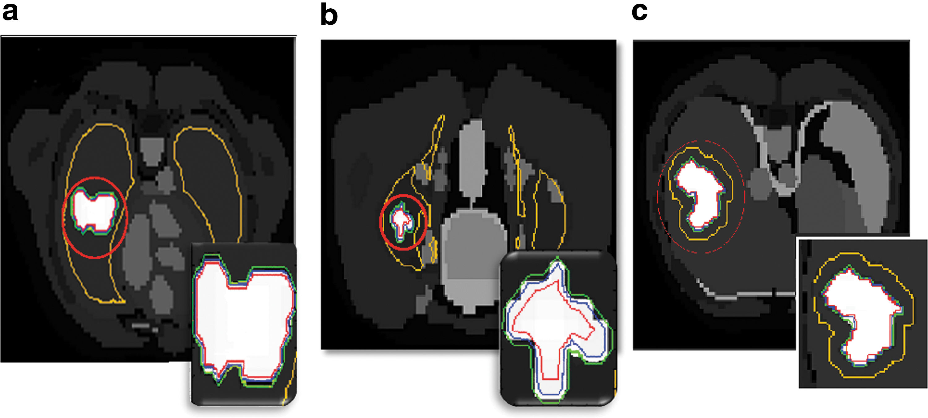
Dose distribution in Zubal phantom. Color-coded isodose contours are superimposed on CT images as follows: red = 75%, blue = 50%, green = 25%, and yellow = 10% of the maximum absorbed dose to the tumors located in (a) lung, (b) bone, and (c) liver. CT, computed tomography. Color images available online at www.liebertpub.com/cbr

Dose volume histograms (DVHs) for the aforementioned organs are generated as shown in Figure 8. These profiles are calculated for the tumor regions based on water and tissue-specific DVKs. The results of comparing two sets of DVHs indicate that the bone and lung DVHs are different from those of water.

FIG. 8.

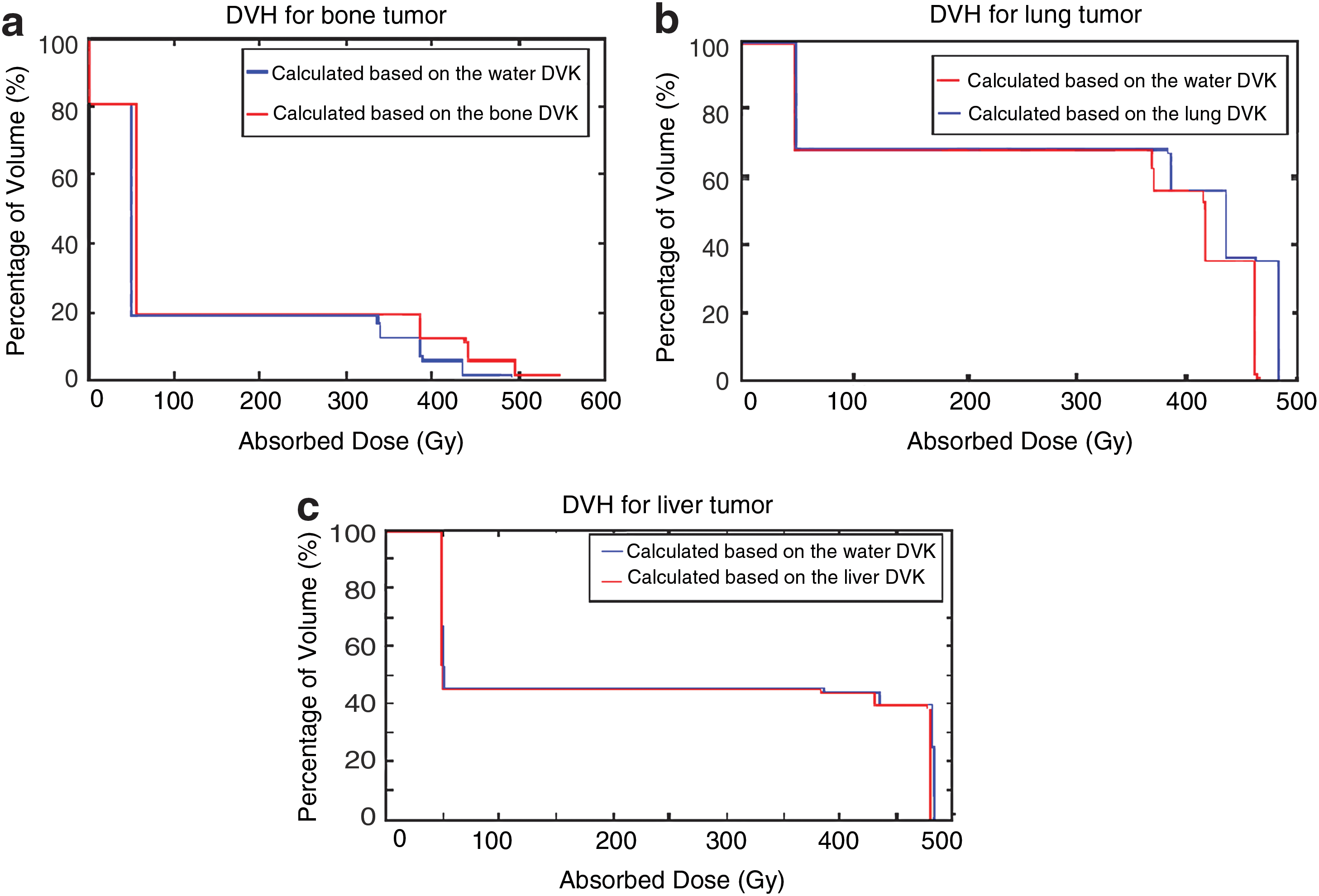
DVHs calculated based on water and tissue-specific DVKs in (a) bone, (b) lung, and (c) liver tumors. DVHs, dose volume histograms; DVKs, dose voxel kernels. Color images available online at www.liebertpub.com/cbr

Dose calculation in heterogeneous medium

To evaluate the impact of tissue heterogeneity on dose distribution, the absorbed dose in a tumor located at bone, lung, and soft tissue boundaries is calculated based on the proposed algorithm and while the Zubal phantom is considered water equivalent. Thereafter, two sets of the achieved results are compared with the absorbed dose calculated using direct MC dosimetry as the reference standard. It was observed that the calculated dose distributions based on the proposed method are in better agreement to those of full MC dosimetry, compared with the conventional methods. In Figure 10a and b, isodose curves calculated based on two aforementioned approaches are superimposed on the corresponding CT images. In Figure 9, DVHs for the tumor located in lung, liver, and bone boundaries based on the aforementioned algorithms and direct MC simulation are shown. The tumor DVH calculated using the proposed algorithm is compared with those of direct MC simulation. The relative difference that is calculated based on the DVH integrals is 12.3%.

FIG. 9.

DVH for the defined tumor in lung, bone, and soft tissue boundaries. Color images available online at www.liebertpub.com/cbr

FIG. 10.

Isodose curves superimposed on CT images. Dose distribution is computed using (a) CT information and (b) Zubal phantom is considered water equivalent. The corresponding line profiles are shown (c). Color-coded isodose contours are as follows: red = 75%, blue = 50%, green = 25%, and yellow = 10% of maximum absorbed dose to the tumor. Color images available online at www.liebertpub.com/cbr

As shown in Figure 10a and b, when water-based DVK is used rather than tissue-specific DVKs, the absorbed dose in normal lung tissue increases. The relative difference between the mean absorbed doses to the tumorous tissue calculated based on our proposed algorithm and those of conventional method is about 6.62%.

Discussion

To estimate activity distributions in a patient with nonuniform spatial distribution of radiotracers, SPECT/CT or PET/CT imaging techniques are used. The determined activity maps thus can be convolved with the appropriate dose kernel to calculate the absorbed dose using both tissue-specific kernels and anatomic data. In this study, tissue-specific DPKs are calculated and compared with water DPKs. Simulation results illustrate the highest mean difference between water and tissue-specific DPKs in bone for ⁹⁰Y (12.2% ± 0.6%), ³²P (18.8% ± 1.3%), and ¹⁷⁷Lu (16.9% ± 1.3%). In lung, the mean differences are 6.3% ± 0.2% for ⁹⁰Y, 8.9% ± 0.4% for ³²P, and 7.7% ± 0.3% for ¹⁷⁷Lu. DPKs of other soft tissues compared with the DPKs of water have lower discrepancies.

The observed differences among various DPKs calculated using different MC codes are a result of various simulation parameters and algorithms in each code. The application of various simulation parameters results in the observed differences between the calculated DPKs in this study and the published data by Papadimitroulas et al. In this study, tissue-specific and water DPKs are simulated using identical simulation parameters and MC code. As such, the observed difference between DPKs of water and other soft tissues in this study corresponds to the statistical uncertainty.

The number of simulated particles for ¹⁷⁷Lu is selected equal to those for ³²P to assess the impact of the energy of β particles on statistical uncertainty. As illustrated in Table 3, although the number of simulated particles for ¹⁷⁷Lu and ³²P is identical, the statistical uncertainty for ¹⁷⁷Lu is worse than that for ³²P at the vicinity of the source and increases faster at farther distance. Radionuclides emitting higher energy particles generate more secondary electrons, so the associated simulation uncertainties are lower. ¹⁷⁷Lu emits low energy β particles, and as such, the number of emitted particles at farther distances decreases rapidly and as a consequence the associated simulation uncertainty increases faster than that for ⁹⁰Y and ³²P.

In contrast, the average energy of ⁹⁰Y and ³²P emitted β particles is approximately in the same order. As such, to assess the impact of increasing the number of emitted particles on statistical uncertainty, the number of ³²P simulated particles are 10 times more than ⁹⁰Y. As shown in Table 3, ³²P-associated statistical uncertainty within its mean range is less than ⁹⁰Y-associated statistical uncertainty at identical distances from the point source.

In internal dosimetry, about 2% discrepancy is neglected because dose estimation is generally associated with further statistical uncertainty, ⁸ and as such, the utilization of water rather than soft tissue DPKs is appropriate. A comparison of tissue-specific DPKs with water DPKs for ⁹⁰Y, ³²P, and ¹⁷⁷Lu is shown in Figure 6.

The higher discrepancies of bone and lung DPKs indicate the importance of considering these organs in personalized dose calculation algorithms. As such, an accurate description of patient anatomy and activity concentration in each voxel should be specified.

Accordingly, we considered tissue-specific DVKs in the dose calculation algorithm in the Zubal phantom for the tumors located in bone, lung, and liver. The achieved results are compared with the calculated absorbed doses, considering the Zubal phantom water equivalent. The highest observed relative difference is about 12.23% for the mean absorbed dose for the tumor located in bone. The relative difference for the tumor in lung tissue of 5.6% is the second and the observed relative difference in mean absorbed dose for liver tumor is about 0.73%. It is observed that the absorbed dose in bone and lung tumors is different from those of water. The observed higher discrepancies are acceptable as the electron densities of bone and lung are significantly different from those of water.⁴³ In contrast, the electron density of the soft tissue is approximately similar to that of water, as such differences between the absorbed doses in soft tissues with those in water are negligible.

In this study, the impact of using bone and lung DVKs instead of water DVKs in the Zubal phantom for ⁹⁰Y is assessed and a new approach for dose calculation is introduced. This method takes tissue heterogeneities and activity inhomogeneity into account and results in a more individualized patient-specific dosimetry. The achieved results based on the proposed algorithm are validated using full MC dosimetry. For the tumor in the heterogeneous region of the Zubal phantom, the relative differences of the mean absorbed dose calculated using full MC dosimetry and the measured dose based on the proposed algorithm and water-equivalent phantom are 5.17% and 12.16%, respectively. Two tailed t-test analysis of the achieved results using the proposed algorithm and direct MC revealed significant statistical difference between estimated absorbed doses to the tumor region (p < 0.001).

In conclusion, the proposed algorithm improves estimation of the average absorbed dose of ⁹⁰Y in a tumor located in lung, bone, and soft tissue interface by 6.98% compared with the conventional methods by taking tissue heterogeneities into consideration, thus enabling patient-specific dosimetry. In general, the average absorbed dose in tumor and nontumor regions shows a very good agreement between the proposed method and the full MC. A point to point comparison of the profiles is illustrated in Figure 10.

To reduce the calculation time, the superimposition algorithm is just used in the interface region for the voxels containing activity. The duration of the computation process using our algorithm is decreased by several orders of magnitude compared with that of full MC simulations.

In Figure 10, isodose curves are superimposed on the CT images of the Zubal phantom, using CT information to account for tissue heterogeneity (Fig. 10a) and considering the Zubal phantom water equivalent (Fig. 10b). The corresponding line profiles are shown in Figure 10c as well. It can be observed that the maximum absorbed dose calculated based on the proposed algorithm is more than that based on conventional methods, because the energy absorption based on the proposed algorithm increases in bone sites, whereas it decreases in lung tissue.

The voxel size of the Zubal phantom is 4 mm and the mean range of ⁹⁰Y β particles in water is about 2.5 mm, thus values of the DVK scored in the voxels surrounding the source voxel significantly have lower contributions on dose distribution than the value of the DVK scored in the central voxel, and the majority of dose is deposited in the source voxel. Consequently, tissue density heterogeneity has a significant influence on the maximum absorbed dose in tumor. The absorbed dose in lung normal tissue, calculated based on water DVKs, is slightly more than the absorbed dose calculated based on tissue-specific DVKs. It indicates that the absorbed dose in lung voxels is overestimated when the Zubal phantom is considered water equivalent.

There are some improvements that can be added to the proposed algorithm. The absorbed dose calculation using our algorithm is based on ⁹⁰Y time-integrated activity in each voxel, assuming that all the administered activity remains in the desired voxel. One of the important features that should be considered in the algorithm is time dependency of absorbed dose as a result of activity distribution variation over time. To account for this, kinetic information of mentioned radionuclides and PET/CT or SPECT/CT images is required. Further work is needed to address the dosimetric impact of the presence of metal in the patient's body.

Conclusions

Individualized treatment planning based on the patient-specific dosimetry improves the quality of radionuclide therapy. Accurate dosimetry methods based on anatomic information has a significant effect on the calculated dose in highly heterogeneous regions. Toward that direction, tissue-specific DPKs for three commonly used radionuclides are generated using Gate MC Toolkit. These DPKs are compared with water DPKs and very good agreement is observed, except for lung and bone. As such it is strongly recommended to consider these organs in dose calculation algorithms. This work contributes to quantify the impact of using tissue-specific DVKs on dose distribution for bone, lung, and soft tissue, as well as to improve dose estimation accuracy through a novel dose calculation algorithm, which takes patient-specific 3D anatomic data into consideration in internal dosimetry. This algorithm improves estimation of the average absorbed dose of ⁹⁰Y in a tumor located in lung, bone, and soft tissue interface by 6.98% compared with the conventional methods by taking tissue heterogeneities into consideration and is a promising technique for patient-specific dosimetry.

Footnotes

Disclosure Statement

No competing financial interests exist.

References

Dewaraja

, Frey

, Sgouros

, et al. MIRD pamphlet No. 23: Quantitative SPECT for patient-specific 3-dimensional dosimetry in internal radionuclide therapy. J Nucl Med, 2012; 53:1310.

Stabin

. Nuclear medicine dosimetry. Phys Med Biol, 2006; 51:R187.

Attarwala

, Molina-Duran

, Busing

, et al. Quantitative and qualitative assessment of Yttrium-90 PET/CT imaging. PLoS One, 2014; 9:e110401.

Bolch

, Bouchet

, Robertson

, et al. MIRD pamphlet No. 17: The dosimetry of nonuniform activity distributions—Radionuclide S values at the voxel level. Medical Internal Radiation Dose Committee. J Nucl Med, 1999; 40:11s.

Lhommel

, van Elmbt

, Goffette

, et al. Feasibility of 90Y TOF PET-based dosimetry in liver metastasis therapy using SIR-Spheres. Eur J Nucl Med Mol Imaging, 2010; 37:1654.

, Lee

, Law

, et al. Patient dosimetry for 90Y selective internal radiation treatment based on 90Y PET imaging. J Appl Clin Med Phys, 2013; 14:212.

Sarfaraz

, Kennedy

, Lodge

, et al. Radiation absorbed dose distribution in a patient treated with yttrium-90 microspheres for hepatocellular carcinoma. Med Phys, 2004; 31:2449.

Papadimitroulas

, Loudos

, Nikiforidis

, et al. A dose point kernel database using GATE Monte Carlo simulation toolkit for nuclear medicine applications: Comparison with other Monte Carlo codes. Med Phys, 2012; 39:5238.

Zavgorodni

. A model for dose estimation in therapy of liver with intraarterial microspheres. Phys Med Biol, 1996; 41:2463.

10.

Loevinger

, Japha

, Brownell

. Discrete Radioisotope Sources. Radiation Dosimctry, 1st ed. New York: Academic Press, 1956.

11.

Spencer

. Theory of electron penetration. Phys Rev, 1955; 98:597.

12.

Berger

. Monte Carlo calculation of the penetration of diffusion of fast charged particles. Meth Comput Phys, 1963; 1:135.

13.

Berger

. Improved Point Kernels for Electron and Beta-Ray Dosimetry (National Bureau of Standards). Washington, DC: National Bureau of Standards, NBSIR, 1973; 73.

14.

Prestwich

, Nunes

, Kwok

. Beta dose point kernels for radionuclides of potential use in radioimmunotherapy. J Nucl Med, 1989; 30:1036.

15.

Strigari

, Menghi

, D'Andrea

, et al. Monte Carlo dose voxel kernel calculations of beta-emitting and Auger-emitting radionuclides for internal dosimetry: A comparison between EGSnrcMP and EGS4. Med Phys, 2006; 33:3383.

16.

Botta

, Mairani

, Battistoni

, et al. Calculation of electron and isotopes dose point kernels with FLUKA Monte Carlo code for dosimetry in nuclear medicine therapy. Med Phys, 2011; 38:3944.

17.

Uusijarvi

, Chouin

, Bernhardt

, et al. Comparison of electron dose-point kernels in water generated by the Monte Carlo codes, PENELOPE, GEANT4, MCNPX, and ETRAN. Cancer Biother Radiopharm, 2009; 24:461.

18.

Jan

, Benoit

, Becheva

, et al. GATE V6: A major enhancement of the GATE simulation platform enabling modelling of CT and radiotherapy. Phys Med Biol, 2011; 56:881.

19.

Maigne

, Perrot

, Schaart

, et al. Comparison of GATE/GEANT4 with EGSnrc and MCNP for electron dose calculations at energies between 15 keV and 20 MeV. Phys Med Biol, 2011; 56:811.

20.

Dieudonne

, Hobbs

, Lebtahi

, et al. Study of the impact of tissue density heterogeneities on 3-dimensional abdominal dosimetry: Comparison between dose kernel convolution and direct Monte Carlo methods. J Nucl Med, 2013; 54:236.

21.

Kwok

, Bialobzyski

, Yu

, et al. Effect of tissue inhomogeneity on dose distribution of point sources of low-energy electrons. Med Phys, 1990; 17:786.

22.

Mikell

, Mahvash

, Siman

, et al. Comparing voxel-based absorbed dosimetry methods in tumors, liver, lung, and at the liver-lung interface for (90)Y microsphere selective internal radiation therapy. EJNMMI Phys, 2015; 2:16.

23.

Sgouros

, Stabin

, Erdi

, et al. Red marrow dosimetry for radiolabeled antibodies that bind to marrow, bone, or blood components. Med Phys, 2000; 27:2150.

24.

Zubal

, Harrell

, Smith

, et al. Computerized three-dimensional segmented human anatomy. Med Phys, 1994; 21:299.

25.

Giap

, Macey

, Bayouth

, et al. Validation of a dose-point kernel convolution technique for internal dosimetry. Phys Med Biol, 1995; 40:365.

26.

Buffa

, Verhaegen

, Flux

, et al. A Monte-Carlo method for interface dosimetry of beta emitters. Cancer Biother Radiopharm, 2003; 18:463.

27.

Charlton

. Energy dissipation near an interface: A more realistic approach to electron range and stopping power. Radiat Res, 1970; 44:575.

28.

Cross

. Variation of beta dose attenuation in different media. Phys Med Biol, 1968; 13:611.

29.

Durham

, Bell

. VARSKIN MOD2 and SADDE MOD2: Computer Codes for Assessing Skin Dose from Skin Contamination. Nuclear Regulatory Commission, 1992; 24, NTIS Issue Number 199309.

30.

Loudos

, Tsougos

, Boukis

, et al. A radionuclide dosimetry toolkit based on material-specific Monte Carlo dose kernels. Nucl Med Commun, 2009; 30:504.

31.

Sanchez-Garcia

, Gardin

, Lebtahi

, et al. A new approach for dose calculation in targeted radionuclide therapy (TRT) based on collapsed cone superposition: Validation with (90)Y. Phys Med Biol, 2014; 59:4769.

32.

ICRP Publication 23. Reference Man: Anatomical, Physiological and Metabolic Characteristics, 1st ed.; Series: Annals of the ICRP (Book 23). SAGE Publications Ltd., 1975.

33.

Measurements ICRU. Tissue Substitutes in Radiation Dosimetry and Measurement. Bethesda, MD: International Commission on Radiation Units and Measurements, 1989.

34.

Jan

, Santin

, Strul

, et al. GATE: A simulation toolkit for PET and SPECT. Phys Med Biol, 2004; 49:4543.

35.

Agostinelli

, Allison

, Amako

, et al. Geant4—A simulation toolkit. Nucl Instrum Meth Phys Res A, 2003; 506:250.

36.

Cross

, Wong

, Freedman

. Dose distributions for electrons and beta rays incident normally on water. Radiat Prot Dosim, 1991; 35:77.

37.

Berger

. Distribution of absorbed dose around point sources of electrons and beta particles in water and other media. J Nucl Med, 1971; Suppl 5:5.

38.

Botta

. Calculation of electron and isotopes dose point kernels with FLUKA Monte Carlo code for dosimetry in nuclear medicine therapy. Med Phys, 2011; 38:3944.

39.

Mainegra-Hing

, Rogers

, Kawrakow

. Calculation of photon energy deposition kernels and electron dose point kernels in water. Med Phys, 2005; 32:685.

40.

Besemer

, Bednarz

. SU-E-T-345: Validation of a patient-specific Monte Carlo targeted radionuclide therapy dosimetry platform. Med Phys, 2014; 41:303.

41.

Carlier

, Eugene

, Bodet-Milin

, et al. Assessment of acquisition protocols for routine imaging of Y-90 using PET/CT. EJNMMI Res, 2013; 3:11.

42.

Ghiron

, Volkert

, Garlich

, et al. Determination of lesion to normal bone uptake ratios of skeletal radiopharmaceuticals by QARG (quantitative autoradiography). Int J Rad Appl Instrum B, 1991; 18:235.

43.

Khan

, Gibbons

. The Physics of Radiation Therapy, 5th ed. Philadelphia, PA: LWW, 2010.

Evaluating the Application of Tissue-Specific Dose Kernels Instead of Water Dose Kernels in Internal Dosimetry: A Monte Carlo Study

Abstract

Purpose:

Materials and Methods:

Results:

Conclusions:

Introduction

Materials and Methods

Calculation of DPKs

Simulation parameters

Dose calculation algorithm in homogeneous medium

Dose calculation algorithm in heterogeneous medium

Validating the proposed algorithm with 90Y

Results

Validation of β particles DPKs

Comparing water DPKs to tissue-specific DPKs

Dose calculation in homogeneous medium

Dose calculation in heterogeneous medium

Discussion

Conclusions

Footnotes

Disclosure Statement

References

Validating the proposed algorithm with ⁹⁰Y