Beyond Dose: Using Pretherapy Biomarkers to Improve Dose Prediction of Outcomes for Radioimmunotherapy of Non-Hodgkin Lymphoma

Abstract

Introduction:

Non-Hodgkin Lymphoma patients respond differently to therapy according to inherent biological variations. Pretherapy biomarkers may improve dose-response prediction.

Materials and Methods:

Hybrid single-photon emission computed tomography (SPECT)/computed tomography (CT) three-dimensional imaging at multiple time points plus follow-up positron emission tomography (PET)/CT or CT at 2 and 6 months post therapy were used to fit tumor response to combined biological effect and cell clearance models from which three biological effect response parameters (radiosensitivity, cold effect sensitivity, and proliferation potential) were determined per patient. A correlation of biological effect parameters and pretherapy biomarker data (ki67, p53, and phospho-histone H3) allowed a dose-based equivalent biological effect (EBE) to be calculated for each patient.

Results:

Significant correlations were found between biological effect parameters and pretherapy biomarkers. Optimum correlations were found by splitting the patient data according to p53 status. Response correlation of progression free survival (PFS) and EBE were significantly improved compared with PFS and absorbed dose alone.

Conclusions:

It is possible and desirable to use pretherapy biomarkers to enhance the predictive potential of dose calculations for patient-specific treatment planning.

Introduction

Afrequent assumption in radiotherapy planning is that all patients of a particular diagnosis will respond identically to a given dose, so that only designing the optimum dose distribution need be considered. However, there is ample evidence that this is not a valid assumption for all diagnoses, particularly for non-Hodgkin lymphomas,^1,2 for which no or limited dose to tumor response correlation has been reported.^2,3 Cicone et al.,⁴ used voxel-based tumor dosimetry to show feasibility and the importance of calculating biological effective dose (BED) and equivalent uniform dose (EUD). Using single-photon emission computed tomography (SPECT) imaging and BED/EUD dose calculation techniques, our group was able to establish a threshold below which a uniformly poor response can be predicted.⁵ Along with this work, biological modeling⁶ and biological parameter development⁷ was accomplished, showing the importance of including the cold effect and proliferation in the prediction of therapeutic response for non-Hodgkin lymphoma.⁸ See Strigari et al.⁹ for a more in depth review of dosimetry developments in the treatment of B cell lymphoma.

To improve therapy planning, we have explored the use of biomarkers to enhance the useful diagnosis of subgroups and thereby create a planning decision tree for use during patient-specific therapy planning. One approach to using biomarkers is to subdivide the patient population based on a threshold biomarker reading, as has been proposed for the use of p53.¹⁰ Another approach is to correlate a biomarker reading with a known patient characteristic, such as proliferation with phospho-histone H3¹¹ or ki67,¹² and p53 with radio-resistance or tumor aggressiveness.^13,14 Our previous work reporting on radiobiological modeling for non-Hodgkin lymphoma suggested correlating radiobiological parameters with biomarkers.⁸ Use of biomarkers for therapy response prediction and radiation treatment planning guidance in non-Hodgkin lymphoma has not been reported. The hypothesis of this study is that improved therapy response prediction can be achieved by accounting for significant cell biological variations among the patient population.

The objective of this study was to use information obtained at diagnosis (e.g., biomarkers sensitive to cell biological variations) and post tracer injection (accumulated antibody exposure estimates) to accurately predict therapy outcome, which is essential for patient-specific therapy planning. Patient imaging data were collected at five or six time points, typically three time points post tracer injection and three post therapy injection. The time and space (four-dimensional) distribution of tumor response history was fit using an equivalent biological effect (EBE) model.^6,7 Each tumor fit provided three parameters, coefficients for terms representing radiosensitivity, cold-effect sensitivity, and proliferation. These parameters were correlated with biomarkers obtained from pretherapy diagnostic biopsies.

The intent of biomarker tests was to determine inherent pretherapy radiosensitivity, cold effect sensitivity, and proliferation potential. Choices for biomarkers were limited because of the requirement for using existing biopsy samples. Biomarkers p53^14

–18 and ki67^19,20 were chosen for radio-/apoptotic sensitivity and proliferation potential, respectively. However, when compared to EBE model parameters, neither biomarker performed as expected. A third biomarker, phospho-histone H3,¹¹ providing more direct sensitivity to proliferation potential, was added to the study. This also added a third reading to correlate with the three EBE model parameters.

Previously, with this data set, we reported a correlation of progression free survival (PFS) with an absorbed dose threshold.⁵ Here, we report on a method to separate patients for whom nondose (i.e., biological) patient attributes affect tumor response to therapeutic dose.

Materials and Methods

Patient characteristics

One hundred forty-eight tumors in 44 relapsed, refractory or upfront non-Hodgkin lymphoma (NHL) patients receiving ¹³¹I Tositumomab (Bexxar) at the University of Michigan between November 2005 and February 2013 were followed. An additional 11 patients enrolled in the study were deleted from the database due to a decision not to treat (4), patient lost to follow-up (6), or initial imaging window not including the tumor (1). The biomarker tests were run on pretherapy biopsy samples taken at diagnosis. Availability of the biopsy samples limited the biomarker study. Initially, tests were performed for ki67 and p53 (37 patients) and later with phospho-histone H3 (24 patients with all three). Of the patients with full biomarker tests performed (ki67, p53, H3), 22 also had biological modeling parameters. Biological modeling parameters for tumors larger than 120 mL were removed from the dataset because they were unreliable estimates due to model assumptions (see Results section). Patient and disease characteristics of the 24 cases used for the outcome analysis are listed in Table 1. The analyzed dataset included diagnoses for diffuse large B cell lymphoma (DLBCL) (21%) and follicular lymphoma (FL) (79%).

Table 1.

Patient and Disease Characteristics

Patient no.	Age	Gender	Diagnosis	Prior treatment	No. of tumors	Baseline volume, ^a mL	Follow-up volume, ^a mL	Mean ^b α, Gy⁻¹	Mean ^b λ_p, g_Tg_P ⁻¹hour⁻¹	Mean ^b λ_t, year⁻¹	% ki67	% p53	% H3	Mean dose, Gy	Mean P, mg_Phg_T ⁻¹ ^c	FU, ^d months	PFS ^e
1	66	m	FL	r^f	1	400^*	529.4				10	0	5	1.71	4.35	1.7	1
2	33	m	FL	r	2	352.9	3.70	1.870	0.7	4.15	30	30	80	4.43	18.4	16.7	1
3	62	f	DLBCL	r	2	104.7	0.00	0.690	280.1	0.25	55	80	35	3.90	13.12	12.2	1
4	48	m	FL	r	6	252.8	73.8	0.388	95.8	0.27	20	30	10	2.17	10.7	7.5	1
5	56	f	FL	r	7	246.6	3.70	1.248	122.0	2.50	50	15	45	3.52	6.71	63.2	0
6	50	f	FL	r	3	63.8	37.80	0.181	115.8	0.66	15	15	70	1.16	3.75	1.9	1
7	52	m	FL	r	3	175.7	23.80	0.818	58.2	0.25	5	0	1	3.99	6.68	26.0	1
8	48	m	FL	r	7	285.1	24.60	0.708	63.3	1.32	70	0	25	3.17	7.60	14.9	1
9	81	m	DLBCL	r	3	6.7	0.00	1.092	7.8	2.50	70	80	45	2.93	5.99	54.2	0
10	67	m	FL	r	7	120.6	18.20	0.220	110.4	0.44	10	0	5	4.70	8.76	4.5	1
11	55	m	FL	r	6	94.4	49.30	0.099	100.7	1.46	15	50	30	2.07	8.17	2.8	1
12	72	m	DLBCL	r	9	65.1	10.90	0.854	128.8	0.78	15	15	10	1.91	7.31	6.5	1
13	73	m	DLBCL	r	5	32.2	0.00	1.728	37.9	2.31	80	25	70	2.92	4.10	11.5	1
14	54	m	FL	r	5	176.5	135.4	0.710	86.5	2.21	35	25	1	2.02	4.05	2.7	1
15	45	m	FL	r	8	117.4	13.7	0.463	42.1	0.29	15	15	15	4.72	8.47	20.4	1
16	40	m	FL	r	4	125.6	6.40	1.047	19.7	0.27	30	5	1	3.03	14.07	25.0	0
17	54	m	FL	u^g	2	12.7	2.70	0.508	13.0	0.68	7.5	5	15	3.32	9.52	23.4	0
18	45	m	FL	u	5	78.6	21.30	0.346	10.8	0.36	5	10	10	4.75	10.87	23.5	0
19	67	m	FL	r	2	167.2	49.10	0.248	71.3	0.25	10	10	25	2.54	33.8	10.8	1
20	79	m	FL	r	2	215.6	297.9	0.284	0.7	1.37	70	15	75	4.10	17.89	1.9	1
21	74	f	FL	u	1	169.9^*	16.02				30	5	50	3.57	12.22	17.8	0
22	63	m	FL	u	3	351.7	168.2	0.277	80.9	1.03	10	0	30	4.48	6.81	3.4	1
23	70	m	DBLCL	r	1	89.7	8.73	0.383	70.4	0.25	20	0	35	4.93	12.08	7.0	0
24	53	m	FL	r	1	46.9	27.68	0.129	351.7	2.87	30	10	80	2.83	5.35	1.8	1

Mean tumor volume at time of therapy or follow-up (∼2 months).

Mean EBE parameter for tumor baselines <120 mL (^* = baselines > 120 mL).

Note units of mg_p instead of g_p used for simplicity of display.

Time of last follow-up.

PFS, 1 = progression, 0 = free of progression.

Relapsed or refractory.

Upfront.

EBE, equivalent biological effect; PFS, progression free survival.

Therapy and imaging protocol

Details of the clinical treatment protocol are given in Kaminski et al.¹ Both tracer (0.2 GBq) and therapy (∼4 GBq) injections used identical antibody mass, a flood dose of 450 mg antibody plus 35 mg of ¹³¹I tagged antibody. Analyses of existing biopsy specimens and the SPECT/computed tomography (CT) imaging protocol for the research study were approved by the University of Michigan Internal Review Board. Each patient provided written informed consent for the analysis and additional imaging: three each (typical) SPECT/CT imaging studies post tracer (days 0, 2, and 5) and post therapy (days 1, 4, and 7) injections. Patients were imaged on a Siemens Symbia TruePoint SPECT/CT scanner (Hoffman Estates, IL) with a six-slice CT capability. A high-energy parallel-hole collimator was used, with 180 (0) and 30 stops per head; 40 seconds per stop; body contouring; 20% photopeak at 364 keV; two adjacent 6% scatter correction windows; and a 128 × 128 matrix with a pixel size of 4.8 mm. The CT used full rotation, 130 kVp, and 35 mAs. The CT dataset yielded a 1 × 1 × 2 mm voxel size. University of Michigan software was used for SPECT/CT expectation maximization (OSEM) using 35 iterations and 6 subsets and included 3D depth dependent resolution recovery.²¹ Recovery coefficients were also used, ranging from 99% to 58% for 100–4 mL volumes, respectively. Follow-up clinical positron emission tomography (PET)/CT (metabolic analysis) or CT (tumor volume analysis) at 2 months and later was used to determine tumor volume and tumor response/progression post therapy.

Dosimetry and biomarker protocol

Registered SPECT/CT data were used to determine voxelized descriptions of tissue densities and activity concentrations, as described by Dewaraja et al.³ SPECT-determined activity distributions and Monte-Carlo calculated three-dimensional (3D) dose rate distributions²² were combined with tumor and rest-of-the-body time-activity curves to yield a position and time-dependent dose rate distribution and antibody concentration distribution for each tumor. Tumor volume contours defined on CT were used to derive the time dependence of tumor volumes for tracer and therapy time intervals. Tumor time-activity data were fit using a bi-exponential function representing the rise and clearance of antibody concentration. Rest-of-the-body (whole body minus tumor) time-activity data were fit using a mono-exponential function representing clearance of antibody concentration.²³ Immunohistochemical studies were performed on paraffin-embedded, archival tissue specimens obtained from patients with a new diagnosis or recurrence of non-Hodgkin lymphoma. The hematopathologist determined the percentage of cells positive for Ki-67, p53, and phospho-histone H3 for each case.

Tumor response model

A combination of an EBE model and a cell clearance model was used to fit absorbed dose sensitivity (α), cold effect sensitivity (λ_p ) and proliferation (λ_t ) parameters, from which equivalent biological effect, E,²⁴ was calculated. Model parameters also included relative tumor volume normalization, effective cell clearance rate (λ_c ), and cell clearance delay for cell inactivation by absorbed dose (t_d ).⁸

EBE model

The EBE, E, is defined as the voxelized cell survival fraction S (v,t), averaged over volume (V), \documentclass{aastex}\usepackage{amsbsy}\usepackage{amsfonts}\usepackage{amssymb}\usepackage{bm}\usepackage{mathrsfs}\usepackage{pifont}\usepackage{stmaryrd}\usepackage{textcomp}\usepackage{portland, xspace}\usepackage{amsmath, amsxtra}\usepackage{upgreek}\pagestyle{empty}\DeclareMathSizes{10}{9}{7}{6}\begin{document} \begin{align*} E = - { \rm{ln}} \left[ {{{ \left< {S \left( {v , t} \right) } \right> }_V}} \right]. \tag{1} \end{align*} \end{document}

Viable cell loss or gain is a function of the biological effective therapy (BET), containing three terms representing radiation effect, cold effect, and proliferation with coeffcients α, λ_p , and λ_t , respectively: \documentclass{aastex}\usepackage{amsbsy}\usepackage{amsfonts}\usepackage{amssymb}\usepackage{bm}\usepackage{mathrsfs}\usepackage{pifont}\usepackage{stmaryrd}\usepackage{textcomp}\usepackage{portland, xspace}\usepackage{amsmath, amsxtra}\usepackage{upgreek}\pagestyle{empty}\DeclareMathSizes{10}{9}{7}{6}\begin{document} \begin{align*} S \left( {v , t} \right) = {e^{ - BET \left( {v , t} \right) }} , \tag{2} \end{align*} \end{document}

\documentclass{aastex}\usepackage{amsbsy}\usepackage{amsfonts}\usepackage{amssymb}\usepackage{bm}\usepackage{mathrsfs}\usepackage{pifont}\usepackage{stmaryrd}\usepackage{textcomp}\usepackage{portland, xspace}\usepackage{amsmath, amsxtra}\usepackage{upgreek}\pagestyle{empty}\DeclareMathSizes{10}{9}{7}{6}\begin{document}$$D \left( {v , t} \right)$$ \end{document} is the cumulative dose, \documentclass{aastex}\usepackage{amsbsy}\usepackage{amsfonts}\usepackage{amssymb}\usepackage{bm}\usepackage{mathrsfs}\usepackage{pifont}\usepackage{stmaryrd}\usepackage{textcomp}\usepackage{portland, xspace}\usepackage{amsmath, amsxtra}\usepackage{upgreek}\pagestyle{empty}\DeclareMathSizes{10}{9}{7}{6}\begin{document}$$RE \left( {v , t} \right)$$ \end{document} is the relative effectiveness accounting for dose-rate dependence, and \documentclass{aastex}\usepackage{amsbsy}\usepackage{amsfonts}\usepackage{amssymb}\usepackage{bm}\usepackage{mathrsfs}\usepackage{pifont}\usepackage{stmaryrd}\usepackage{textcomp}\usepackage{portland, xspace}\usepackage{amsmath, amsxtra}\usepackage{upgreek}\pagestyle{empty}\DeclareMathSizes{10}{9}{7}{6}\begin{document}$$P \left( {v , t} \right)$$ \end{document} is the antibody concentration residence time, in grams of antibody protein times hour per gram of tumor.

The cold-effect term is proportional to \documentclass{aastex}\usepackage{amsbsy}\usepackage{amsfonts}\usepackage{amssymb}\usepackage{bm}\usepackage{mathrsfs}\usepackage{pifont}\usepackage{stmaryrd}\usepackage{textcomp}\usepackage{portland, xspace}\usepackage{amsmath, amsxtra}\usepackage{upgreek}\pagestyle{empty}\DeclareMathSizes{10}{9}{7}{6}\begin{document} \begin{align*} P \left( { v , t } \right) = { \frac { { P_ { inj } } } { { A_ { inj } } \cdot \rho V } } \mathop \int \limits_0^t A \left( { v , t \prime } \right) \cdot { e^ { \gamma \cdot t \prime } } dt \prime , \tag { 4 } \end{align*} \end{document}

where \documentclass{aastex}\usepackage{amsbsy}\usepackage{amsfonts}\usepackage{amssymb}\usepackage{bm}\usepackage{mathrsfs}\usepackage{pifont}\usepackage{stmaryrd}\usepackage{textcomp}\usepackage{portland, xspace}\usepackage{amsmath, amsxtra}\usepackage{upgreek}\pagestyle{empty}\DeclareMathSizes{10}{9}{7}{6}\begin{document}$${P_{inj}}$$ \end{document} and \documentclass{aastex}\usepackage{amsbsy}\usepackage{amsfonts}\usepackage{amssymb}\usepackage{bm}\usepackage{mathrsfs}\usepackage{pifont}\usepackage{stmaryrd}\usepackage{textcomp}\usepackage{portland, xspace}\usepackage{amsmath, amsxtra}\usepackage{upgreek}\pagestyle{empty}\DeclareMathSizes{10}{9}{7}{6}\begin{document}$${A_{inj}}$$ \end{document} are the quantity of antibody mass and activity at time of injection, \documentclass{aastex}\usepackage{amsbsy}\usepackage{amsfonts}\usepackage{amssymb}\usepackage{bm}\usepackage{mathrsfs}\usepackage{pifont}\usepackage{stmaryrd}\usepackage{textcomp}\usepackage{portland, xspace}\usepackage{amsmath, amsxtra}\usepackage{upgreek}\pagestyle{empty}\DeclareMathSizes{10}{9}{7}{6}\begin{document}$$\rho V$$ \end{document} is the tumor mass in g, and \documentclass{aastex}\usepackage{amsbsy}\usepackage{amsfonts}\usepackage{amssymb}\usepackage{bm}\usepackage{mathrsfs}\usepackage{pifont}\usepackage{stmaryrd}\usepackage{textcomp}\usepackage{portland, xspace}\usepackage{amsmath, amsxtra}\usepackage{upgreek}\pagestyle{empty}\DeclareMathSizes{10}{9}{7}{6}\begin{document}$$A \left( {v , t \prime } \right) \cdot {e^{ \gamma \cdot t \prime }}$$ \end{document} is the decay-corrected activity distribution.

Cell clearance model

The time dependence of the tumor volume, \documentclass{aastex}\usepackage{amsbsy}\usepackage{amsfonts}\usepackage{amssymb}\usepackage{bm}\usepackage{mathrsfs}\usepackage{pifont}\usepackage{stmaryrd}\usepackage{textcomp}\usepackage{portland, xspace}\usepackage{amsmath, amsxtra}\usepackage{upgreek}\pagestyle{empty}\DeclareMathSizes{10}{9}{7}{6}\begin{document} \begin{align*} Z \left( t \right) = \mathop \sum \limits_V Z \left( {v , t} \right) , \tag{5} \end{align*} \end{document}

has two components, an inactivated (but not yet cleared) cell volume, \documentclass{aastex}\usepackage{amsbsy}\usepackage{amsfonts}\usepackage{amssymb}\usepackage{bm}\usepackage{mathrsfs}\usepackage{pifont}\usepackage{stmaryrd}\usepackage{textcomp}\usepackage{portland, xspace}\usepackage{amsmath, amsxtra}\usepackage{upgreek}\pagestyle{empty}\DeclareMathSizes{10}{9}{7}{6}\begin{document}$${C_z} \cdot U ( v , t )$$ \end{document} , and a viable cell volume, \documentclass{aastex}\usepackage{amsbsy}\usepackage{amsfonts}\usepackage{amssymb}\usepackage{bm}\usepackage{mathrsfs}\usepackage{pifont}\usepackage{stmaryrd}\usepackage{textcomp}\usepackage{portland, xspace}\usepackage{amsmath, amsxtra}\usepackage{upgreek}\pagestyle{empty}\DeclareMathSizes{10}{9}{7}{6}\begin{document}$${C_z} \cdot N \left( {v , t} \right)$$ \end{document} , \documentclass{aastex}\usepackage{amsbsy}\usepackage{amsfonts}\usepackage{amssymb}\usepackage{bm}\usepackage{mathrsfs}\usepackage{pifont}\usepackage{stmaryrd}\usepackage{textcomp}\usepackage{portland, xspace}\usepackage{amsmath, amsxtra}\usepackage{upgreek}\pagestyle{empty}\DeclareMathSizes{10}{9}{7}{6}\begin{document} \begin{align*} Z \left( {v , t} \right) = {C_z} \cdot \left[ {U \left( {v , t} \right) + N \left( {v , t} \right) } \right] , \tag{6} \end{align*} \end{document}

where C_z is the volume per cell. The time dependence of Z is \documentclass{aastex}\usepackage{amsbsy}\usepackage{amsfonts}\usepackage{amssymb}\usepackage{bm}\usepackage{mathrsfs}\usepackage{pifont}\usepackage{stmaryrd}\usepackage{textcomp}\usepackage{portland, xspace}\usepackage{amsmath, amsxtra}\usepackage{upgreek}\pagestyle{empty}\DeclareMathSizes{10}{9}{7}{6}\begin{document} \begin{align*} Z \left( { v , t } \right) = Z \left( { v , 0 } \right) + { C_z } \cdot \left[ { \mathop \int \limits_0^t \left( { { \frac { dU \left( { v , t \prime } \right) } { dt \prime } } \left. { + { \lambda _t } \cdot N ( v , t \prime } \right) } \right) dt \prime } \right] , \tag { 7 } \end{align*} \end{document}

where the first term is the initial volume and the terms in the bracket represent cell loss and cell proliferation. The proliferation term is proportional to the number of viable cells. Cell loss has two components, loss due to the radiation effect and loss due to the cold effect. \documentclass{aastex}\usepackage{amsbsy}\usepackage{amsfonts}\usepackage{amssymb}\usepackage{bm}\usepackage{mathrsfs}\usepackage{pifont}\usepackage{stmaryrd}\usepackage{textcomp}\usepackage{portland, xspace}\usepackage{amsmath, amsxtra}\usepackage{upgreek}\pagestyle{empty}\DeclareMathSizes{10}{9}{7}{6}\begin{document} \begin{align*}{{dU \left( {v , t} \right) } \over {dt}} = - { \lambda _c} \left[ { \mathop \int \limits_{{\ t_d}}^t {e^{ - { \lambda _c} \cdot \left( {t- t \prime } \right) }} \cdot \alpha \cdot} \right.\\ \left.{{{d \left[{D \left( {v , {t^ \prime } - {t_d}} \right) \cdot RE \left( {v , t \prime - {t_d}} \right) } \right] } \over {dt \prime }} \cdot N \left( {v , t \prime - {t_d}} \right) \cdot dt \prime} \right.\\ \left.{+ \mathop \int \limits_0^t {e^{ - { \lambda _c} \cdot \left( {t - t \prime } \right) }} \cdot { \lambda _p} \cdot {{dP \left( {v , t \prime } \right) } \over {dt \prime }} \cdot N \left( {v , t \prime } \right) \cdot dt \prime } \right] , \tag{8} \end{align*} \end{document}

where the cell clearance constant, \documentclass{aastex}\usepackage{amsbsy}\usepackage{amsfonts}\usepackage{amssymb}\usepackage{bm}\usepackage{mathrsfs}\usepackage{pifont}\usepackage{stmaryrd}\usepackage{textcomp}\usepackage{portland, xspace}\usepackage{amsmath, amsxtra}\usepackage{upgreek}\pagestyle{empty}\DeclareMathSizes{10}{9}{7}{6}\begin{document}$${ \lambda _c}$$ \end{document} , can be related to clearance half-time, \documentclass{aastex}\usepackage{amsbsy}\usepackage{amsfonts}\usepackage{amssymb}\usepackage{bm}\usepackage{mathrsfs}\usepackage{pifont}\usepackage{stmaryrd}\usepackage{textcomp}\usepackage{portland, xspace}\usepackage{amsmath, amsxtra}\usepackage{upgreek}\pagestyle{empty}\DeclareMathSizes{10}{9}{7}{6}\begin{document}$${T_c} ,$$ \end{document} \documentclass{aastex}\usepackage{amsbsy}\usepackage{amsfonts}\usepackage{amssymb}\usepackage{bm}\usepackage{mathrsfs}\usepackage{pifont}\usepackage{stmaryrd}\usepackage{textcomp}\usepackage{portland, xspace}\usepackage{amsmath, amsxtra}\usepackage{upgreek}\pagestyle{empty}\DeclareMathSizes{10}{9}{7}{6}\begin{document} \begin{align*}{ \lambda _c} = \ln \left( 2 \right) / {T_c} , \tag{9} \end{align*} \end{document}

and t_d is the clearance delay imposed for the observed delay in cell clearance for the radiation effect.

We assume that at t = 0, the tumor volume is composed entirely of viable cells, and that the time dependence of the volume of viable cells is proportional to the cell survival curve, \documentclass{aastex}\usepackage{amsbsy}\usepackage{amsfonts}\usepackage{amssymb}\usepackage{bm}\usepackage{mathrsfs}\usepackage{pifont}\usepackage{stmaryrd}\usepackage{textcomp}\usepackage{portland, xspace}\usepackage{amsmath, amsxtra}\usepackage{upgreek}\pagestyle{empty}\DeclareMathSizes{10}{9}{7}{6}\begin{document}$$Z \left( {v , 0} \right) = {C_z} \cdot N \left( {v , 0} \right)$$ \end{document} and \documentclass{aastex}\usepackage{amsbsy}\usepackage{amsfonts}\usepackage{amssymb}\usepackage{bm}\usepackage{mathrsfs}\usepackage{pifont}\usepackage{stmaryrd}\usepackage{textcomp}\usepackage{portland, xspace}\usepackage{amsmath, amsxtra}\usepackage{upgreek}\pagestyle{empty}\DeclareMathSizes{10}{9}{7}{6}\begin{document}$$ { \frac { N \left( { v , t } \right) } { N \left( { v , 0 } \right) } } = S \left( { v , t } \right)$$ \end{document} . Additional information has been previously published.^6
–8

Time-dependent voxelized tumor volume

Tumor volumes were defined on CT and registered over time with deformable registration using center of mass alignment and radial deformation. Voxels from the initial scan were tracked in subsequent scans by fixing the number and relative positions of voxels for all time points. The tumor time-activity curves at the voxel level followed the curve for the tumor as a whole. Because the 3D activity distributions changed between time points, the time-activity curves at the voxel level, midway between time points was discontinuous. Dose rates followed the position and time dependence of the activity distribution. 3D voxelized tumor dose rates were calculated with a self-absorbtion term due to tumor activity and a rest-of-the-body term due to the rest-of-the-body activity. This was done to allow the time history of the dose rates and total (voxelized) tumor dose to be calculated using the voxelized self-absorbed tumor dose rates with the tumor time-activity curve plus the rest-of-body tumor dose rates with rest-of-body time-activity curve.

The calculated time dependence of the tumor volume (Equation 6) was compared to the (five or) six measured CT-defined volumes and the 2-month follow-up volume. The 2-month volume was used to help fix the proliferation parameter (λ_t ). Model fit parameters were radiosensitivity (α), cold-effect sensitivity (λ_p ), proliferation rate (λ_t ), effective cell clearance rate (λ_c ), cell clearance delay for cell inactivation by radiation effect (t_d ), and tumor volume normalization. Model inputs were dose rate and activity distributions and tumor volumes. Model outputs were the fit parameters and E. Tumor volume normalization was used as a fitted parameter because of observed variability of the day 0 tumor volumes compared to days 2 and 5 volumes. By allowing the tumor volume normalization to vary, tumor volume errors at all times were treated equally. Tumor volume data were normalized to 1 at t = 0 for data fitting convenience.

Least squares EBE and cell clearance model fitting

Initially, parameters were limited to finite ranges to avoid nonphysical local minima. Fitting was performed in two steps. In a first step, fitting varied tumor volume normalization and λ_p , keeping other parameters at nominal values. In a second step, fitting was performed keeping tumor volume normalization and λ_p fixed and optimizing α, λ_t , λ_c , and t_d within the chosen intervals. Fitting was performed at least twice per tumor, iteratively for the first and second steps, using the previous best-fit parameters as initial values. To avoid local minima, multiple overlapping intervals for t_d were chosen based on the observed time of rapid tumor volume decrease following the therapeutic injection. Some tumors required a refitting with an alternative t_d interval with the best final fit chosen. A small overlap between t_d intervals helped determine the best-fit values without danger of a local minimum trap. Example tumor shrinkage fits are shown in Figure 1.

FIG. 1.

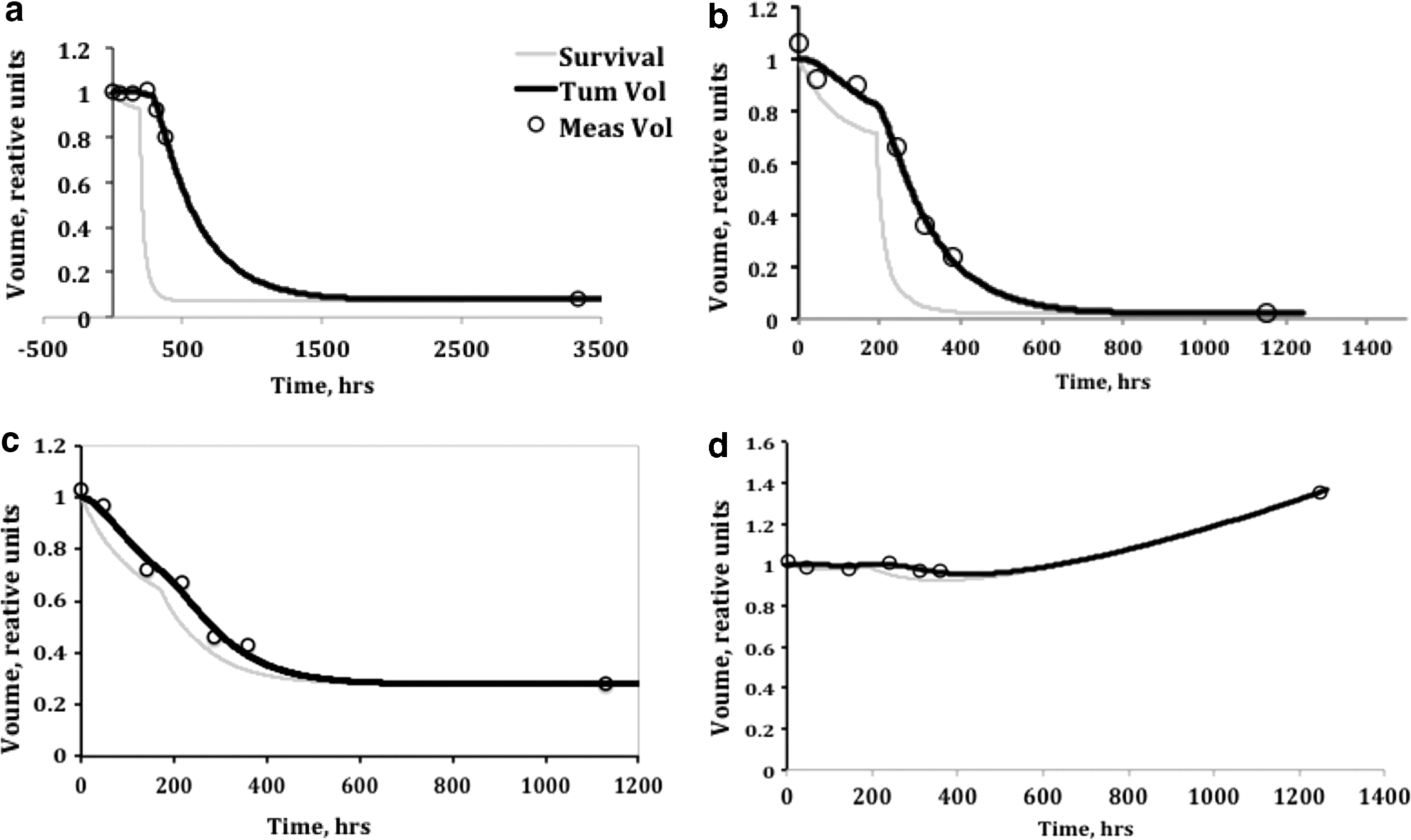
Example tumor shrinkage fitting. Shown are tumor volume history fits for examples with (a) no cold effect with high radiosensitivity, (b) high cold effect with high radiosensitivity, (c) high cold effect with low radiosensitivity, and (d) high proliferation. Plotted are relative cell survival, calculated tumor volume, and measured tumor volume.

Correlation between biomarker data and EBE parameters and between E or dose and 2-month tumor shrinkage data was determined using linear regression. Statistical significance was calculated using a t-test applied to the square of the correlation coefficient. Correlation of E with the CT 2-month shrinkage was used to estimate relative quality of the fitting procedures. The log of the ratio of the 2-month tumor volume to the initial volume was plotted against E. Complete response at 2 months (i.e., tumor volume not observed on CT) was plotted using approximately half of the minimum detectable volume, 0.25 mL.

Biomarker data fitting

Fitted EBE model parameters were averaged over studied tumors for each patient. Tumor number per patient ranged from 1 to 7. Linear least square fitting of the biomarker data to the model parameters was performed. In matrix form, \documentclass{aastex}\usepackage{amsbsy}\usepackage{amsfonts}\usepackage{amssymb}\usepackage{bm}\usepackage{mathrsfs}\usepackage{pifont}\usepackage{stmaryrd}\usepackage{textcomp}\usepackage{portland, xspace}\usepackage{amsmath, amsxtra}\usepackage{upgreek}\pagestyle{empty}\DeclareMathSizes{10}{9}{7}{6}\begin{document} \begin{align*} \left[ { \begin{matrix} {{{ \left\{ \alpha \right\} }_1}} & {{{ \left\{ {{ \lambda _p}} \right\} }_1}} & {{{ \left\{ {{ \lambda _t}} \right\} }_1}} \\ \cdots & \cdots & \cdots \\ {{{ \left\{ \alpha \right\} }_n}} & {{{ \left\{ {{ \lambda _p}} \right\} }_n}} & {{{ \left\{ {{ \lambda _t}} \right\} }_n}} \\ \end{matrix} } \right] = \end{align*} \end{document} \documentclass{aastex}\usepackage{amsbsy}\usepackage{amsfonts}\usepackage{amssymb}\usepackage{bm}\usepackage{mathrsfs}\usepackage{pifont}\usepackage{stmaryrd}\usepackage{textcomp}\usepackage{portland, xspace}\usepackage{amsmath, amsxtra}\usepackage{upgreek}\pagestyle{empty}\DeclareMathSizes{10}{9}{7}{6}\begin{document} \begin{align*} \left[ { \begin{matrix} 1 & {{{ \left\{ {ki67} \right\} }_1}} & { \begin{matrix} {{{ \left\{ {p53} \right\} }_1}} & {{{ \left\{ {H3} \right\} }_1}} \\ \end{matrix} } \\ \cdots & \cdots & { \begin{matrix} \cdots & {} \\ \end{matrix} \cdots } \\ 1 & {{{ \left\{ {ki67} \right\} }_n}} & { \begin{matrix} {{{ \left\{ {p53} \right\} }_n}} & {{{ \left\{ {H3} \right\} }_n}} \\ \end{matrix} } \\ \end{matrix} } \right] \left[ { \begin{matrix} {a1} & {b1} & {c1} \\ {a2} & {b2} & {c2} \\ { \begin{matrix} { a3} \\ {a4} \\ \end{matrix} } & { \begin{matrix} { b3} \\ {b4} \\ \end{matrix} } & { \begin{matrix} {c3} \\ {c4} \\ \end{matrix} } \\ \end{matrix} } \right] , \tag{10} \end{align*} \end{document}

where {x}_i is the average parameter or average biomarker for patient i and the matrix [a1 … c4] contains best fit values. These matrices were then used to calculate best-fit patient-specific (predictive) model parameters. Biomarker-predicted parameters {α, λ_p , λ_t } were determined using Equation (10), using the biomarker data and the best-fit matrix values.

Predicted model parameters were used to form a predicted E for each patient, \documentclass{aastex}\usepackage{amsbsy}\usepackage{amsfonts}\usepackage{amssymb}\usepackage{bm}\usepackage{mathrsfs}\usepackage{pifont}\usepackage{stmaryrd}\usepackage{textcomp}\usepackage{portland, xspace}\usepackage{amsmath, amsxtra}\usepackage{upgreek}\pagestyle{empty}\DeclareMathSizes{10}{9}{7}{6}\begin{document} \begin{align*}{ \left[ {E \left( t \right) } \right] _{pred}} = { \left[ \alpha \right] _{pred}} \cdot {D_{ave}} + { \left[ {{ \lambda _p}} \right] _{pred}} \cdot {P_{ave}} - { \left[ {{ \lambda _t}} \right] _{pred}} \cdot t , \tag{11} \end{align*} \end{document}

Predicted parameters for a future patient could be calculated by setting n = 1 in Equation (10) and using the biomarker readings from pretherapy biopsies. Predicted E values could be calculated from Equation (11), obtaining the predicted parameters from Equation (10) and predicted D_ave and P_ave from a tracer study.

Progression free survival

PFS was defined as the minimum time to progression, relapse, or death from any cause and was calculated from the date of the tracer administration. Patients alive and without evidence of progression, on the last date of assessment, were censored as of that date. The Kaplan–Meier method was used to summarize PFS times for all patients and for various comparison groups. Because predicted E parameters are derived from patient tumor shrinkage data, for the PFS analysis each patient's predicted E was derived from data of the remaining study patients using Equations (10) and (11). Kaplan–Meier analyses were used to compare the predictive potential of E versus absorbed dose.

Statistics

Data set comparisons assume parametric statistics and normal distributions (Figs. 2 and 3; Tables 3 and 4). Kaplan–Meier analyses were performed using MedCalc (MedCalc Software, Ostend, Belgium; www.medcalc.org) and nonparametric statistics.

FIG. 2.

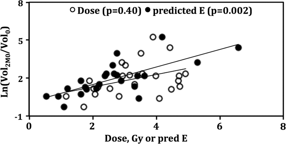
Fitted versus predicted parameters, correlation coefficient and significance for (a) radiosensitivity, (b) cold effect sensitivity, and (c) proliferation rate.

FIG. 3.

Dose and predicted E (2 months) versus tumor shrinkage. Correlation coefficient R ² = 0.17 and 0.54 for dose and predicted E, respectively. The p53 groups are analyzed as one group to determine the correlation.

Results

One to nine (average four) tumor histories were fit per study patient using the EBE and cell clearance models. Each fit yielded model parameter estimates. For patients with more than one studied tumor, the model parameters (α, λ_p , λ_t ) were averaged to yield optimum values per patient. While some variability in derived parameters was observed, parameters for most study patients were clustered relative to the full dataset. Patient biomarkers available were dependent on biopsy sites chosen during diagnosis and could not be identified with specific tumor locations.

The EBE model parameter dataset used for biomarker fitting was limited to tumor sizes of 0–120 mL. Larger tumor data contained significant outliers, degrading the biomarker fit quality. This was attributed to the assumptions of the EBE model (i.e., constant exponential tumor growth and uniform cell oxic conditions) that were not appropriate for larger tumors with likely inadequate blood supply, hypoxia, and/or necrosis. The use of the biomarkers to predict parameters was applied to all patients in the dataset. Thus, there were two more patients in the predicted dataset compared to the fit dataset, representing two patients with all (one or more) tumors above the 120 mL threshold.

Correlations between biomarker data and EBE parameters were determined using linear least-square fits yielding a correlation coefficient that can be related to a probability of significance (p value). No correlations between biomarkers ki67 and p53 and parameters were observed for the grouped dataset. Although ki67 is generally used for identifying proliferation, it is an indirect test of proliferation. It has also been found to identify a quiescent state of non-Hodgkin lymphoma, potentially frustrating a direct correlation with proliferation potential (see Discussion section). To improve the correlation potential, a biomarker for direct proliferation detection was added (phospho-histone H3). Phospho-histone H3 data correlated with the proliferation parameter (correlation coefficient 0.416, p = 0.02). H3 data did not significantly correlate with the other EBE model coefficients or with ki67.

The biomarker p53 has been used by others as an indicator of loss of cell cycle control. The database was split into groups with likely cell cycle control (p53 ≤ 15%) and likely loss of control (p53 > 15%). Significant (p < 0.05) correlations were found for H3 with the radiosensitivity parameter for p53 > 15%, and H3 with proliferation parameter for p53 ≤ 15%. Correlation coefficients generally improved for the radiosensitivity and proliferation rate parameters. Using p53 as a dataset discriminator was superior to using diagnosis or any other observed criteria.

A linear matrix fit was used to determine the best fit between the three biomarkers and the EBE parameters for the two groups. The matrix fit yielded improved correlations for all parameters and significant correlation for two of the three parameters (p < 0.001, 0.08, and <0.001 for α, λ_p , and λ_t , respectively). Correlation plots are given in Figure 2a–c. Fit matrices are presented in Table 2. Alternative p53 discrimination levels yielded less significant correlation (e.g., only λ_t correlation was significant at p = 0.008 for 10% discrimination). For this dataset, a p53 discrimination value of 20% is identical to the 15% value chosen.

Table 2.

Biomarker—Equivalent Biological Effect Model Parameter Fit Matrices

	α, Gy⁻¹	λ_P, g_Tg_P ⁻¹hour⁻¹	λ_t, year⁻¹
P53 ≤ 15%
constant	0.4773	0.0597	0.3591
ki67	0.9306	−0.1173	3.1805
p53	1.5854	−0.1659	0.1510
H3	−1.0506	0.2217	4.4005
P53 > 15%
constant	0.3560	0.0645	4.1464
ki67	1.004	−0.0189	−1.0500
p53	−0.9701	0.1724	−4.2245
H3	1.5228	−0.1240	8.7463

Biomarkers expressed as fractional values.

While both groups included a range of biomarker and parameter values mean values of radiosensitivity and proliferation rate differed by about a factor of 2 (Table 3). Comparing p53-split groups, mean proliferation rates were significantly different (p = 0.03); mean radiosensitivities were marginally different (p = 0.11); and mean cold sensitivities were not different.

Table 3.

Group Average Predicted Equivalent Biological Effect Model Parameters

p53	No. in group	α, Gy⁻¹	λ_P, g_Tg_P ⁻¹hour⁻¹	λ_t, year⁻¹
p53 ≤ 15%	15	0.51 (0.24)^a	84 (49)	0.89 (0.60)
p53 > 15%	7	0.94 (0.62)	87 (57)	1.88 (0.98)
p ^b		0.11	—	0.032

Mean (standard deviation of the sample).

Probability of null hypothesis for two-tailed t distribution.

The 2-month shrinkage value was used during EBE parameter determinations. However, comparing the predicted outcome against the 2-month shrinkage can be used as a consistency test of the data analysis method. Biomarker-derived predicted E values determined at 2 months showed an improved correlation with tumor 2-month shrinkage compared with absorbed dose alone (Fig. 3). The p53 ≤ 15% group correlation with 2-month shrinkage improved from absorbed dose alone (p = 0.61) to predicted E (p = 0.27). There was little change in the p53 > 15% group (p = 0.01 and 0.02 for dose and predicted E, respectively). However, the combined group improved from not significant (p = 0.40) for absorbed dose alone to significant (p = 0.002) for predicted E (Table 4).

Table 4.

Dose Versus Predicted E (2 Months) Correlation with 2-Month Shrinkage

	No. in group	Dose	Predicted E (2 months)
p53 ≤ 15%	15	p = 0.61; R ² = 0.13	p = 0.27; R ² = 0.25
p53 > 15%	7	p = 0.01; R ² = 0.81	p = 0.02; R ² = 0.76
All	24	p = 0.40; R ² = 0.17	p = 0.002; R ² = 0.54

Progression free survival

Correlation of dose or predicted E with PFS was used to compare the predictive power of E with that of absorbed dose. For each patient, a separate predicted parameter analysis was performed using the dataset minus that patient's data. For predicted model parameters less than zero, their values were reset to zero (2 and 1 of 24 for λ_p and λ_t , respectively). The time parameter was used to weaken or strengthen the proliferation term in the predicted E formula (Equation 11). The optimum correlation with PFS was found for t = 18 months.

Improved performance for predicted E was obtained by applying a time discriminator on the proliferation coefficient. For patients with lower proliferation [λ_t <1.6 year⁻¹ or potential doubling time (T_pot ) > 160 day], a low time value was used in Equation (11), retaining the excellent correlation observed with dose alone at low dose or predicted E values. Significant improvement in correlation with PFS for the higher proliferation cases required a large time value (∼18 months), affecting 5 of 24 (21%) of patients. The high proliferation cases were split 3–2 between low and high p53 subgroups. To illustrate the PFS correlation improvement in a manner less dependent on this particular dataset, a sigmoid rather than a threshold time function was chosen (Fig. 4). Kaplan–Meier graphs are shown for the even (12,12) patient split, for absorbed dose (Fig. 5a) and predicted E (Fig. 5b). The improvement was statistically significant, with the p values of 0.081 (absorbed dose alone) and 0.0003 (predicted E). Mean PFS was 15.7 and 25.9 months for the low and high dose groups and 6.0 and 34.1 months for the low and high predicted E groups, respectively. The median PFS was 7.5 and 20.4 months for the low and high dose groups compared to 2.8 and 26.0 months for the low and high predicted E groups. Hazard ratios for the high/low groups were 0.44 and 0.21 for dose and predicted E, respectively.

FIG. 4.

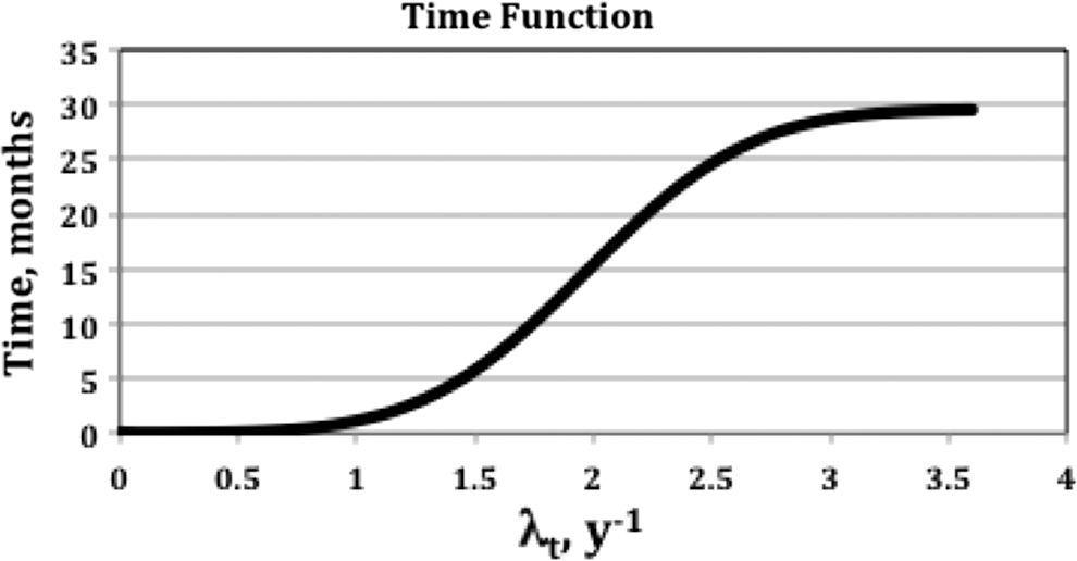
Time for evaluation of E as a function of the proliferation coefficient.

FIG. 5.

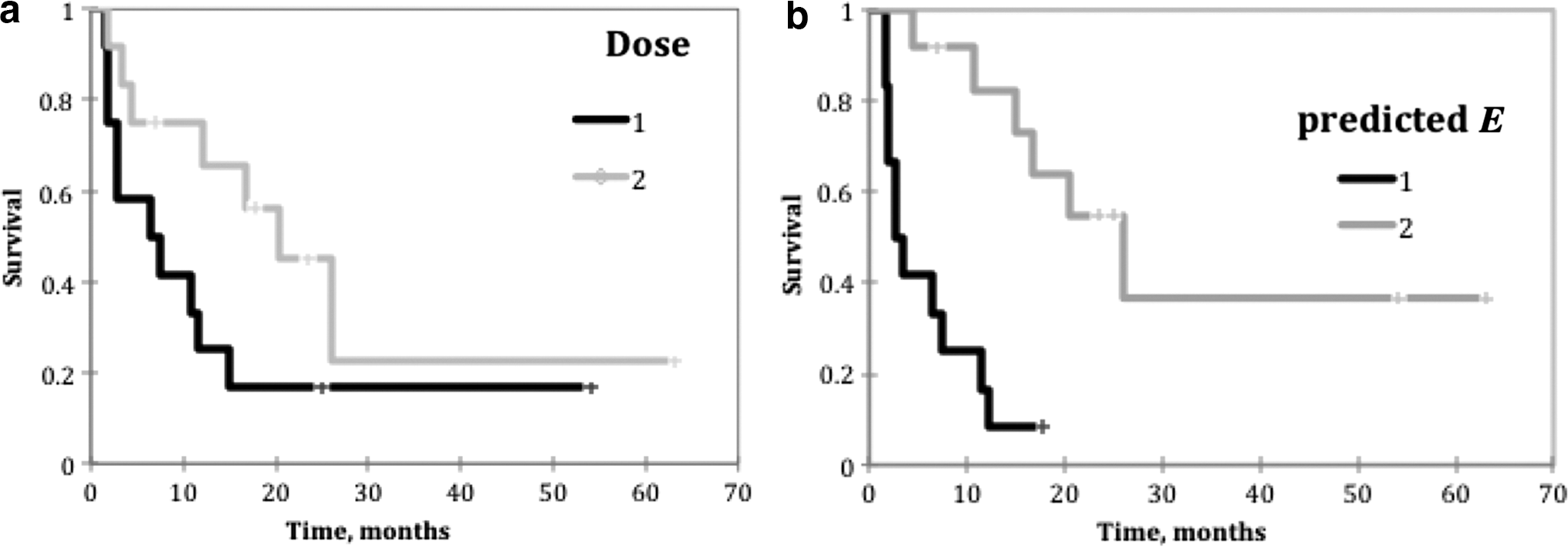
Kaplan–Meier graphs for a (12,12) patient split using (a) dose split <3.2 Gy (curve 1) or >3.2 Gy (curve 2) (p = 0.081); and (b) predicted E(t) split <2.0 (curve 1) or >2.0 (curve 2) (p = 0.0003).

A more complete picture of the comparison of dose to predicted E was obtained by calculating the correlation significance in groupings of patients. Patients were ordered by increasing dose or predicted E values, for increasing lower group numbers from (6,18) to (18,6) splits. Calculated p values were used to quantify the quality of the outcome predictor at each level. Dose correlation with PFS was excellent for the lower doses (p < 0.01), while no correlation with PFS (p > 0.7) was observed at higher doses (see dose curve in Fig. 6). The optimum correlation with PFS for a fixed time value (t = 18 months) is shown in the “Predicted E, 18 mo” curve in Figure 6. Low predicted E values correlated less well with PFS compared with low doses, although both were at a significant level. Higher predicted E values correlated with PFS compared to no correlation with higher doses. Optimum predicted E performance using the variable time curve from Figure 4 is also shown (E, variable t), indicating comparable performance at low values and significantly improved performance at higher values. Significant correlation of predicted E with outcome was extended to higher E values compared to the t = 18 months curve.

FIG. 6.

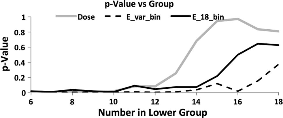
Kaplan–Meier p values as a function of group size from (6,18) to (18,6) for dose, predicted E(t) at t = 18 months, and predicted E(t) at t = variable time using time as a function of proliferation coefficient, λ_t , given in Figure 4.

Discussion

Biomarker correlation with model parameters

Non-Hodgkin lymphoma, as its name implies, is a collection of similar diseases. The origin of non-Hodgkin lymphoma is believed to be gene translocations occurring within bone marrow.²⁵ Further, p53 mutations in FL cells result in diffuse large B cell lymphoma (DLBCL). Thus, a diagnosis of FL can progress to large B cell lymphoma over time. Other non-Hodgkin lymphoma types are due to alternative gene translocations.

Biomarker p53 provided the most critical patient-specific information, enabling the separation of the patient population into two distinct groups with substantially different responses to therapy. This separation was key in demonstrating an outcome prediction advantage for E over dose alone. Since absorbed dose is a component of E, if radiosensitivity did not significantly vary and cold effect and proliferation were not significant outcome contributors, then at best, E would perform the same as dose.

High p53 implies the presence of mutant p53 and the loss of some cell cycle control.¹⁴ Cell proliferation is more likely to be out of control (high proliferation rate) and higher proliferation implies higher radiosensitivity. Contrary to expectations of using p53 to predict the presence of apoptosis (and possibly the strength of the cold effect), it was primarily used to separate groups of average lower and higher radiosensitivity-proliferation performance (Table 3).

The model performed poorly when the dataset was split based on diagnosis (FL vs. DLBCL) rather than p53 biomarker. The dataset was too small to apply diagnosis-based and p53-based splits. The poor performance for a diagnosis split may be partially due to the transforming nature of the FL-DLBCL relationship. However, the present patient group is also highly selected, most being referred for radioimmunotherapy postfailure of alternative therapies.

The ki67 test is sensitive to the fraction of cells not in the G0 (resting) state. For most cell lines, the results are synonymous with active proliferation. However, ki67 is also known to express in noncycling cells that are arrested in a non-G0 state, particularly cells that overexpress p53.^18,19 Since some FL cell populations are known to exist in a non-G0 state for extended periods of time,²⁵ the ki67 test can simultaneously detect two interesting conditions: presence of a quiescent non-G0 state and high proliferation potential. Note that high proliferation potential tends to predict poor therapeutic outcome, while large numbers of cells in quiescent state tends to predict a good outcome. To counter this ambiguity, Phosphohistone H3 was used as a more direct measure of mitosis. Thus, for the cells under active control (p53 ≤ 15%), ki67 marginally and H3 significantly correlate with proliferation rate and work together to detect proliferation potential (positive coefficients in Table 2), resulting in a highly significant correlation with radiosensitivity and proliferation rate. For cell populations with some loss of cell cycle control (p53 > 15%), H3 correlated with radiosensitivity (p = 0.03). H3 also worked along with ki67 to separate high proliferation potential from quiescent abnormal cell behavior (negative coefficient for a₂₃ with positive coefficient for a₄₃ in Table 2). In this case, ki67 and H3 work together to improve the correlation with radiosensitivity (p = 0.003).

Alternative biomarkers may provide additional information to add to or better define the properties of tumors at the time of therapy. This study was limited to preserved biopsy samples taken at diagnosis. Future studies designed to better define biomarker-enhanced therapy planning could use fresh biopsy samples allowing alternative biomarker collection, such as proliferating cell nuclear antigen expression in flow cytometry assays.²⁶

Predicted E

The data analysis used a fully 3D and time-dependent description to derive model parameters, providing optimal parameter estimates. The cutoff for inclusion in the biomarker fit of 120 mL tumor volume was an indirect confirmation that the parameter estimates were consistent far above the imaging resolution (∼12 mL tumor volume). The need for a tumor volume cutoff was more indicative of the failure of the present EBE model to correctly account for large tumor response (shrinkage) without accounting for confounding factors, such as necrosis or inefficient vasculature. The goal of the EBE model fitting was an accurate determination of the relative strengths of the three terms in the predicted E formula through the determination of the term coefficients. The final calculation used a simplified formula for predicted E, requiring estimates of average dose and average P, obtainable from a tracer study, in addition to the parameter estimates derivable from biomarkers. The simplified estimate of predicted E is similar to the logic of calculating an average dose as a therapy response marker from a 3D time-dependent analysis.

Progression free survival

Comparison of the predictive value for therapy effectiveness was performed with PFS, an accepted outcome marker²⁷ independent of the data analysis used to form dose and predicted E. Using accurate modeling, predicted E would always outperform dose because predicted E includes dose and other known significant varying biological properties of patient tumors, namely radiation sensitivity, cold effect sensitivity, and proliferation rate. However, this was not generally the case probably due to variability of the derived parameters using low patient numbers. For instance, for the proliferation to be weighted properly for patients with high proliferation potential, the time value had to be large (∼18 months). Whereas, for patients with lower proliferation potential, a higher time value added a considerable amount of noise in the predicted E formula, degrading the response correlation for patients where proliferation was low enough to not affect outcome. Statistical error in parameter calculations also resulted in a few nonphysical values (less than zero) when analyzed for the 14- or 6-patient calculations used for the PFS analysis. These were set to zero to prevent statistical error in one parameter from negating an observed response in another.

The time value was tested in 3-month intervals from t = 3 months to t = 30 months. The preference for t = 18 months over 15 or 21 months was small, but more significant compared to times further afield. To obtain the optimum results for this patient set, using a variable time in the E formula was likely needed due to statistical error in the determination of the optimal model parameters. The preference for ∼18 months can be seen in Figure 5, where the two survival curves have the greatest separation for both dose and predicted E.

Where dose correlated well, there were two model discriminators required to prevent altering the performance of predicted E from that of absorbed dose alone. The primary discriminator was p53 threshold of 15% to separate tumors with different cell cycle control allowing a better estimate of radiosensitivity. The secondary discriminator was time in the E formula used to identify and penalize high proliferation potential. The most important concept was to avoid degrading the quality of the dose response where it appeared to work well, while identifying patient tumors with high radiosensitivity and/or high proliferation potential. Optimal results identified patients that had good performance markers (high dose and/or high radiosensitivity) and poor performance markers (high proliferation potential). High proliferation potential correlated uniformly with the poorest results, no matter the dose or radiosensitivity. Higher radiosensitivity or higher dose correlated with improved outcome, working separately or together.

Conclusions

It is possible and desirable to separate patient populations using pretherapy biomarkers. Potential treatment planning advantages are (1) to avoid low-dose, slow acting therapies (such as radioimmunotherapies) for some aggressive tumors; (2) to explore dose and dose-rate escalation in tumors that may be close to improved response; and (3) to continue with current therapy for those where it is optimal. The biomarkers explored here were chosen from well-established techniques to help define particular patient tumor properties. The relationship of the biomarkers to patient response was complex and required considerable disentanglement using detailed EBE calculations. This was likely due to the heterogeneous patient mix. Use of the EBE model allowed an improved interpretation of the significance of the biomarker readings, and ultimately may lead the way for improved therapy outcome prediction and patient-specific treatment planning.

Footnotes

Acknowledgment

This work was supported by grant NIH 2R01 EB001994 awarded by the National Institutes of Health, United States Department of Health and Human Services.

Disclosure Statement

Dr. Kaminski receives research support from GlaxoSmithKline and royalties from Bexxar. All other authors have no conflict of interest.

References

Kaminski

, Estes

, Zasadny

, et al. Radioimmunotherapy with iodine ¹³¹I tositumomab for relapsed or refractory B-cell non-Hodgkin Lymphoma: Updated results and long-term follow-up of the University of Michigan experience. Blood, 2000; 96:1259–1266.

Sgouros

, Squeri

, Ballangrud

, et al. Patient-specific, 3-dimensional dosimetry in non-Hodgkin's lymphoma patients treated with 131i-ANTI-B1 antibody: Assessment of tumor dose-response. J Nucl Med, 2003; 44:260–268.

Dewaraja

, Schipper

, Roberson

, et al. I-131 tositumomab radioimmunotherapy: Initial tumor dose-response results using 3-D dosimetry including radiobiological modeling. JNM, 2010; 51:1155–1162.

Cicone

, D'Arienzo

, Carpaneto

, et al. Quantification of dose nonuniformities by voxel-based dosimetry in patients receiving 90Y-ibritumomab-tiuxetan. Cancer Biother Radiopharm, 2013; 28:98–107.

Dewaraja

, Schipper

, Shen

, et al. Tumor-absorbed dose predicts progression-free survival following 131I-tositumomab radioimmunotherapy. J Nucl Med, 2014; 55:1047–1053.

Amro

, Wilderman

, Dewaraja

, et al. Methodology to incorporate biologically effective dose and equivalent uniform dose in patient-specific 3-dimensional dosimetry for non-Hodgkin lymphoma patients targeted with 131I-tositumomab therapy. J Nucl Med, 2010; 51:654–659.

Roberson

, Amro

, Wilderman

, et al. Bio-effect model applied to 131I radioimmunotherapy of refractory non-Hodgkin's lymphoma. Eur J Med Mol Imaging, 2011; 38:874–883.

Roberson

, Wilderman

, Avram

, et al. Biological-effect modeling of radioimmunotherapy for non-hodgkins lymphoma: Determination of model parameters. Cancer Biother Radiopharm, 2014; 29:26–33, 2014.

Strigari

, Konijnenberg

, Chiesa

, et al. The evidence base for the use of internal dosimetry in the clinical practice of molecular radiotherapy. Eur J Nucl Med Mol Imaging, 2014; 41:1976–1988.

10.

Fernandez-Pol

, Ma

, Ohgami

, et al. Immunohistochemistry for p53 is a useful tool to identify cases of acute myeloid leukemia with myelodysplasia-related changes that are TP53 mutated, have complex karyotype, and have poor prognosis. Mod Pathol, 2017; 30:382–392.

11.

Sun

, Zhou

, Lunceford

, et al. Level of phosphohistone H3 among various types of human cancers. BMJ Open, 2012; 2:e001071.

12.

Sviatoha

, Tani

, Rassidakis

, et al. Analysis of proliferating cell fraction determined by monoclonal antibody to M1-subunit ribonucleotide reductase and Ki-67 in relation to p53 protein expression in fine-needle aspirates from non-Hodgkin's lymphomas. Cytopathology, 2000; 11:290–301.

13.

Stefancikova

, Moulis

, Fabian

, et al. Loss of the p53 tumor suppressor activity is associated with negative prognosis of mantle cell lymphoma. Int J Oncol, 2010; 36:699–706.

14.

Villuendas

, Piris

, Orradre

, et al. P53 protein expression in lymphomas and reactive lymphoid tissue. J Pathol, 1992; 166:235–241.

15.

Dahm-Daphi

. p53: Biology and role for cellular radiosensitivity. Strahlenther Onkol, 2000; 176:278–285.

16.

Pervez

, Nasir

, Moatter

, et al. Characterization of genetic lesions in apoptosis-regulating and proliferation control genes in diffuse large B-cell non-Hodgkin's lymphoma. J Can Res Ther, 2009; 5:254–262.

17.

Chatzitolios

, Venizelos

, Tripsiannis

, et al. Prognostic significance of CD95, P53, and BCL2 expression in extranodal non-Hodgkin's lymphoma. Ann Hematol, 2010; 89:889–896.

18.

Bhatt

, Mathur

, Farooque

, et al. Cancer biomarkers—Current perspectives. Indian J Med Res, 2010; 132:129–149.

19.

Van Oijen

, Medema

, Slootweg

, et al. Positiviity of the proliferation marker Ki-67 in noncycling cells. Am J Clin Pathol, 1998; 110:24–31.

20.

Koster

, Tromp

, Raemaekers

JMM

, et al. The prognostic significance of the intra-follicular tumor cell proliferative rate in follicular lymphoma. Haematologica, 2007; 92:184–190.

21.

Koral

, Yendiki

, Dewaraja

. Recovery of total I-131 activity within focal volumes using SPECT and 3D OSEM. Phys Med Biol, 2007; 52:777–790.

22.

Wilderman

, Dewaraja

. Method for fast CT/SPECT-based 3D Monte Carlo absorbed dose computations in internal emitter therapy. IEEE Trans Nucl Sci, 2007; 54:146–151.

23.

Schipper

, Koral

, Avram

, et al. Prediction of therapy tumor-absorbed dose estimates in I-131 radioimmunotherapy using tracer data via a mixed-model fit to time activity. Cancer Biother Radiopharm, 2012; 27:403–411.

24.

Dale

. The application of the linear-quadratic dose-effect equation to fractionated and protracted radiotherapy. Br J Rad, 1985; 58:515–528.

25.

Kluin

, Han

, van Krieken

. Malignant lymphomas stem from different B cell populations. Chem Immunol, 1997; 67:70–84.

26.

Sawtell

, Rew

, Stradling

, et al. Pan cycle expression of proliferating cell nuclear antigen in human colorectal cancer and its proliferative correlations. Cytometry, 1995; 22:190–199.

27.

Korn

, Crowley

. Overview: Progression-free survival as an endpoint in clinical trials with solid tumors. Clin Cancer Res, 2013; 19:2607–2612.