Data Structures for Parsimony Correlation and Biosequence Co-Evolution

Abstract

We give an algorithm for discovering co-evolution in biosequences from a dataset consisting of aligned data and a phylogeny. The method correlates vectors of parsimony scores on the edges of a graph, averaged over all optimally parsimonious reconstructions of the data. We describe an efficient data structure, and a preprocessing step that allows for rapid, interactive computation of many correlation scores, at the expense of storage space.

1. Introduction

Understanding the networks of interactions between molecules and/or portions of molecules in an organism is of fundamental importance in modern biology. Understanding gene-gene interactions (Glazier et al., 2002), gene-protein interactions (Li et al., 2007), protein-protein interactions (Tamayo et al., 2008), and so on is necessary when trying to understanding how healthy organisms operate, and to find cures when they become unhealthy. Such work is often done in the lab using time-consuming and expensive techniques. Biologists are increasingly interested in employing computational aids that will assist in the search for pairs of molecules that interact with one another.

One approach to discovering such interacting pairs is based on the observation that two molecules which interact tend also to evolve together, a process called co-evolution. Any method which allows us to quantify evolution also allows us to measure co-evolution, and therefore make conjectures about interaction. This has been done, for example in Ramani and Marcotte (2003), using similarity matrices, in Kim et al. (2006), using mutual information, and in Jothi et al. (2005), using tree topology, respectively, to quantify evolution and co-evolution.

In the present paper, we use parsimony scores to quantify evolution, and correlation of vectors of scores to quantify co-evolution. We also use a pre-processing step to allow for rapid computation of correlations.

2. The Parsimony Graph

We begin with a precise description of the problem, which may be thought of as an abstract problem on strings. Let \documentclass{aastex}\usepackage{amsbsy}\usepackage{amsfonts}\usepackage{amssymb}\usepackage{bm}\usepackage{mathrsfs}\usepackage{pifont}\usepackage{stmaryrd}\usepackage{textcomp}\usepackage{portland, xspace}\usepackage{amsmath, amsxtra}\pagestyle{empty}\DeclareMathSizes{10}{9}{7}{6}\begin{document} $$A = \{ a_{1}, \ldots, a_{k}\}$$ \end{document} be some finite alphabet, and X be a string of length n over A. We will denote by X[i] the ith character of X (i ranges from 1 to n) and by X[i, j] the substring of X from X[i] to X[j], 1 ≤ i ≤ j ≤ n. A rooted binary tree T is a tree with k nodes of degree one (the leaves), one node of degree 2, (the root), and k − 2 nodes of degree 3, for some k ≥ 2. When we write an edge (v,w) of T, we will adopt the convention that the first vertex, v, is the parent, that is, the vertex closer to the root, and w is the child, further from the root than v. Thus each edge will be written in the order (parent, child).

Let \documentclass{aastex}\usepackage{amsbsy}\usepackage{amsfonts}\usepackage{amssymb}\usepackage{bm}\usepackage{mathrsfs}\usepackage{pifont}\usepackage{stmaryrd}\usepackage{textcomp}\usepackage{portland, xspace}\usepackage{amsmath, amsxtra}\pagestyle{empty}\DeclareMathSizes{10}{9}{7}{6}\begin{document} $$S = \{ S_{1}, S_{2}, \ldots, S_{k}\}$$ \end{document} be a set of finite strings, all of length n, let T be a rooted binary tree with k leaves \documentclass{aastex}\usepackage{amsbsy}\usepackage{amsfonts}\usepackage{amssymb}\usepackage{bm}\usepackage{mathrsfs}\usepackage{pifont}\usepackage{stmaryrd}\usepackage{textcomp}\usepackage{portland, xspace}\usepackage{amsmath, amsxtra}\pagestyle{empty}\DeclareMathSizes{10}{9}{7}{6}\begin{document} $$l_{1}, \ldots, l_{k}$$ \end{document} and let the strings be associated bijectively with the leaves, so that string S_i is “on” leaf l_i. This corresponds biologically to molecules found in species at the leaves of the tree, which evolved from some common ancestor at the root. Denote by S[i, j] the collection of substrings \documentclass{aastex}\usepackage{amsbsy}\usepackage{amsfonts}\usepackage{amssymb}\usepackage{bm}\usepackage{mathrsfs}\usepackage{pifont}\usepackage{stmaryrd}\usepackage{textcomp}\usepackage{portland, xspace}\usepackage{amsmath, amsxtra}\pagestyle{empty}\DeclareMathSizes{10}{9}{7}{6}\begin{document} $$\{ S_{1} [ i, \ j], S_{2} [ i, \ j], \ldots, S_{k} [ i, \ j]\}$$ \end{document} . We will call such collections domains. Figure 1 illustrates these concepts. What we wish to find are domains which have co-evolved with each other.

Fig. 1.

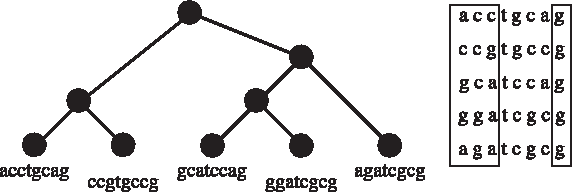
A rooted binary tree with five leaves, and the strings on those leaves. Two domains in these sequences, S[1, 3] of size 3 and S[8, 8] of size 1, are shown to the right.

2.1. Parsimony

The art of inferring the evolutionary histories of species that we see in the present is called phylogenetic reconstruction, and consists of constructing a hypothetical tree describing the speciation events that took place as they evolved from a common ancestor, and constructing hypothetical sequences on the non-leaf nodes in the tree representing best guesses as to what the molecules might have been in those ancestors. In this paper, we will assume that a tree has been found already, and will concentrate solely on reconstructing and studying the ancestral sequences. Of course, any such reconstruction represents nothing more than an educated guess. So we use the notion of parsimony to decide which guesses are better than others, and then select the best.

Parsimony Idea: Given a phylogenetic tree T, with vertices V(T) and edges E(T), let the vertices be labeled with equal length strings of characters and let v_j denote the value of the jth character of vertex v ∈ V(T). Then the parsimony cost is defined as \documentclass{aastex}\usepackage{amsbsy}\usepackage{amsfonts}\usepackage{amssymb}\usepackage{bm}\usepackage{mathrsfs}\usepackage{pifont}\usepackage{stmaryrd}\usepackage{textcomp}\usepackage{portland, xspace}\usepackage{amsmath, amsxtra}\pagestyle{empty}\DeclareMathSizes{10}{9}{7}{6}\begin{document} \begin{align*}pc ( T) = \sum\limits_{( v, u)\, \in\, E( T\, )} \mid \{ \, j \, : \, v_{j} \ne u_{j}\} \mid \tag{1}\end{align*} \end{document}

Notice that, in the computation of pc(T), we compare the j th character of any string only with the jth characters in other strings, so that, if we let Δ (x, y) = 0 if x = y and 1 otherwise, then \documentclass{aastex}\usepackage{amsbsy}\usepackage{amsfonts}\usepackage{amssymb}\usepackage{bm}\usepackage{mathrsfs}\usepackage{pifont}\usepackage{stmaryrd}\usepackage{textcomp}\usepackage{portland, xspace}\usepackage{amsmath, amsxtra}\pagestyle{empty}\DeclareMathSizes{10}{9}{7}{6}\begin{document} \begin{align*}pc( T) = \sum\limits_{( v, u)\, \in\, E( T)} \mid \{\, j \, : \, v_{j} \ne u_{j}\} \mid = \sum\limits_j \ \sum\limits_{( v, u)\, \in\, E( T)} \Delta \, ( u_j, v_j),\end{align*} \end{document}

and our computations may be done on one character at a time. Let us therefore assume that the strings on the leaves are all of length one, and that we seek to find a single character for each internal node to minimize the total parsimony cost. Such an assignment will be called a reconstruction. This problem was solved by Fitch in 1971, but we will not use his method here (Fitch, 1971). Rather, we will take a dynamic programming approach similar to that used by Blanchette (2002).

2.2. Dynamic programming

The quantity we wish to consider is the following: For each node v of the tree and each x ∈ A, what is the minimal cost we could realize on the subtree consisting of v and its descendents (relative to the root of T) if we placed x on node v? We denote this cost by c(v_x). For example, for the alphabet {a, c, g, t} and the tree shown in Figure 2, we have c(u_a) = c(u_c) = 1 and c(u_g) = c(u_t) = 2, while c(w_a) = 1, c(w_g) = 2 and c(w_c) = c(w_t) = 3.

Fig. 2.

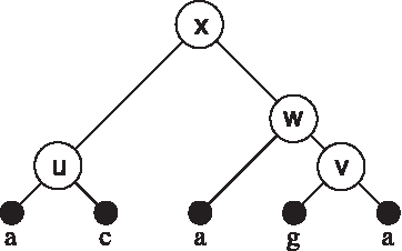
The labels on the leaves of the tree, and the names of the internal nodes, are shown.

Let us introduce a data structure called a parsimony graph, whose vertices are {v_x|v ∈ V (T), x ∈ A}, and whose edges we will define shortly. The shape of this graph is roughly that of the shape of T, but with each vertex of T replaced by k “character vertices.” Thus, the node v_x would represent the placement of character x ∈ A on node v, and c(v_x) would be the cost defined above. We observe that the value c(v_x) depends on the values of c(w_y) for each child w of v in T and each y ∈ A. In particular, if w^L and w^R are the left and right children of v in T, then \documentclass{aastex}\usepackage{amsbsy}\usepackage{amsfonts}\usepackage{amssymb}\usepackage{bm}\usepackage{mathrsfs}\usepackage{pifont}\usepackage{stmaryrd}\usepackage{textcomp}\usepackage{portland, xspace}\usepackage{amsmath, amsxtra}\pagestyle{empty}\DeclareMathSizes{10}{9}{7}{6}\begin{document} \begin{align*}c ( v_x) = \min\limits_{y \, \in \, A}( c \, ( w^{ L}_{y}) + \Delta_{xy}) + \min\limits_{y \, \in \, A}( c \, ( w^{ R}_{y}) + \Delta_{x y}) \tag{2}\end{align*} \end{document}

where Δ_xy = 0 if x = y, and 1 otherwise. (This is 1 − δ_xy, where δ is the usual Kronecker delta function.) To see why equation (2) holds consider the best cost that can be obtained by placing character x on node v. For each label y that could be used on the left child w^L we obtain a cost of 0 on the edge (v,w^L) if y = x, and a cost of 1 otherwise. Additionally, we consider the minimal cost of the subtree of w^L when w^L is labeled with y. Finally, we take the minimum over all choices for y. Independently we make the same computation on the right subtree, and add together the two minimal costs. The “base cases” on the leaves are treated as follows: \documentclass{aastex}\usepackage{amsbsy}\usepackage{amsfonts}\usepackage{amssymb}\usepackage{bm}\usepackage{mathrsfs}\usepackage{pifont}\usepackage{stmaryrd}\usepackage{textcomp}\usepackage{portland, xspace}\usepackage{amsmath, amsxtra}\pagestyle{empty}\DeclareMathSizes{10}{9}{7}{6}\begin{document} \begin{align*}c \ (v_x) = \begin{cases}0 \qquad {\rm if \it v} {\prime} {\rm s \ given \ label \ is} \ x \\ \infty \qquad {-}\end{cases}\tag{3}\end{align*} \end{document}

We use ∞ to signify that we may not use a different character than that given.

2.3. Adding the edges

The parsimony graph is simply the memoization step of the dynamic program described above. In particular, if v has children w^L and w^R in T and \documentclass{aastex}\usepackage{amsbsy}\usepackage{amsfonts}\usepackage{amssymb}\usepackage{bm}\usepackage{mathrsfs}\usepackage{pifont}\usepackage{stmaryrd}\usepackage{textcomp}\usepackage{portland, xspace}\usepackage{amsmath, amsxtra}\pagestyle{empty}\DeclareMathSizes{10}{9}{7}{6}\begin{document} $$c( v_x) = c( w_y^L) + \Delta_{xy}$$ \end{document} , then we draw an edge from v_x to w_y in the parsimony graph. Thus every character vertex v_x of the parsimony graph will have at least one edge to at least one character vertex \documentclass{aastex}\usepackage{amsbsy}\usepackage{amsfonts}\usepackage{amssymb}\usepackage{bm}\usepackage{mathrsfs}\usepackage{pifont}\usepackage{stmaryrd}\usepackage{textcomp}\usepackage{portland, xspace}\usepackage{amsmath, amsxtra}\pagestyle{empty}\DeclareMathSizes{10}{9}{7}{6}\begin{document} $$w_{y}^{L}$$ \end{document} , and also at least one edge to some character vertex \documentclass{aastex}\usepackage{amsbsy}\usepackage{amsfonts}\usepackage{amssymb}\usepackage{bm}\usepackage{mathrsfs}\usepackage{pifont}\usepackage{stmaryrd}\usepackage{textcomp}\usepackage{portland, xspace}\usepackage{amsmath, amsxtra}\pagestyle{empty}\DeclareMathSizes{10}{9}{7}{6}\begin{document} $$w_{y{\prime}}^{R}$$ \end{document} . The parsimony graph for the tree in Figure 2 is shown in Figure 3. ( Biological Note: Frequently, the root in a phylogenetic tree is a theoretical construct, not an actual species, and therefore would not properly receive its own character in an optimal reconstruction. In particular, if a reconstruction gives two different characters to the root's two children, then our algorithm would generate two different optimal reconstructions, one for each of those characters placed on the root. To avoid getting two trees in this case, we force the root to have the same character as its right child, by removing from the parsimony graph those edges \documentclass{aastex}\usepackage{amsbsy}\usepackage{amsfonts}\usepackage{amssymb}\usepackage{bm}\usepackage{mathrsfs}\usepackage{pifont}\usepackage{stmaryrd}\usepackage{textcomp}\usepackage{portland, xspace}\usepackage{amsmath, amsxtra}\pagestyle{empty}\DeclareMathSizes{10}{9}{7}{6}\begin{document} $$( r_{x}, r_{y}^{R})$$ \end{document} where x ≠ y. Thus, the parsimony graph shown in Figure 3 would have three of the edges from the root to its right child deleted.)

Fig. 3.

The parsimony graph for the tree shown in Figure 2, over the alphabet {a, c, g, t}. The circled characters show the labels given on the leaves, and the numbers show the costs c(v_x) for placing character x on node v in the tree.

A glance at the parsimony graph reveals much about the optimal reconstructions. First of all, the only optimal choice for the root of the tree is “a,” as that yields cost 2 while all other character choices yield higher cost. Furthermore, following the edges down from character “a” at the root, we find that its left child must be labeled with “a” also, since no edge goes to any other character there. Similarly, the right child must be labeled with “a,” and its right child must be labeled with “a.” In this fashion, the parsimony graph encodes all optimal reconstructions. In our example, there was just a single optimal selection. In general, the number of optimal reconstructions may be exponential in the number of leaves, but the parsimony graph will always have |A||V(T)| nodes and no more than |A|² · (|V(T)| − 1) edges. That is, for any fixed alphabet A, the graph size will be linear in the number of leaves of the tree.

2.4. Average parsimony vectors

The parsimony graph allows us to compute the number of optimal reconstructions as well. Again we use dynamic programming, but we re-use the memos (edges) already computed above. For each character node v_x, let us define n(v_x) to be the number of optimal reconstructions of the subtree of T rooted at v, given that character x is used on node v. Then \documentclass{aastex}\usepackage{amsbsy}\usepackage{amsfonts}\usepackage{amssymb}\usepackage{bm}\usepackage{mathrsfs}\usepackage{pifont}\usepackage{stmaryrd}\usepackage{textcomp}\usepackage{portland, xspace}\usepackage{amsmath, amsxtra}\pagestyle{empty}\DeclareMathSizes{10}{9}{7}{6}\begin{document} \begin{align*} \begin{split}\hbox{For leaves} \quad n( v_{x}) = \begin{cases}1 \hbox{if} \qquad v \ {\rm is \ labeled \ with \ x} \\ 0 \qquad {-}\end{cases} \\ \\ \hbox{For internal nodes} \quad n( v_{x}) = \left(\sum\limits_{ y \, \in \, A} n( w^{\, L}_y)\right)\cdot \left(\sum\limits_{y \, \in \, A} n( w^{\, R}_y)\right)\end{split} \tag{4} \end{align*} \end{document}

where w^L and w^R are the children of v in T. Equation (4) says that the number of trees is the product of the number of optimal left subtrees times the number of optimal right subtrees, since they may be selected independently. The number of optimal reconstructions for the whole tree is then given by \documentclass{aastex}\usepackage{amsbsy}\usepackage{amsfonts}\usepackage{amssymb}\usepackage{bm}\usepackage{mathrsfs}\usepackage{pifont}\usepackage{stmaryrd}\usepackage{textcomp}\usepackage{portland, xspace}\usepackage{amsmath, amsxtra}\pagestyle{empty}\DeclareMathSizes{10}{9}{7}{6}\begin{document} \begin{align*}\hbox{Number of Optimal Reconstructions} = \sum_{ \textstyle{y\, \in\, A \atop c ( r_y) \ {\rm minimal}}} n \, ( r_y)\tag{5}\end{align*} \end{document}

where r is the root of the tree. This computation can be done in time linear in the number of leaves, even including the step of building the parsimony graph in the first place. Finding this number in linear time was also done in Rinsma et al. (1990) using generating functions.

Given an optimal reconstruction, we may place on each edge (v,w) of T a value 0 or 1 according as v and w get the same or different characters, respectively, in that reconstruction. If we order the edges of T, then this placement becomes a binary vector. The ordering we use is a “post-ordering” of the edges, where each edge (v,w) gets a number only after the left and right subtrees of w have been numbered, in that order. We call this ordering of the edges a “post-ordering” because it arises from a traditional post-ordering of the vertices by moving the number on each vertex to the edge above it. (We use a post-ordering because it places the edge from the root to its right child last. As described in Section 2.3, this edge will always have cost 0, and will therefore contribute nothing to our correlations. We may therefore ignore the last component of the vector, retaining only the initial 2k − 3 components.) From an evolution point of view, this vector may be thought of as a cross-section of the evolutionary history of the domain. It indicates those times when a change took place in the sequence comprising that molecule. If we find another molecule whose changes correlate with the changes in this molecule, we may see that as evidence that the molecules have co-evolved.

Prior to correlating, however, we have two considerations: First, there may be more than one optimal reconstruction, and second, that each domain may have length greater than one. Longer domains are easily handled by our previous observation that the parsimony cost of a domain is simply the sum of the parsimony costs of the individual positions in that domain. But handling the plurality of optimal reconstructions presents a whole research area in itself. For example, a tree with 15 leaves and 200 optimal reconstructions can be thought of as a set of 200 binary vectors in 27-dimensional space, and we need some way to correlate such a point set with another point set of the same dimension but perhaps of a different size. In this paper we represent the set of vectors by the average of the vectors, giving us just a single vector of floating point numbers representing a domain, so that correlating two domains can be done by correlating two vectors. But one could use Tukey depth (Tukey, 1975) or any of the other notions of data depth to identify some central point to use as a representative of the domain. We have not made any explorations in this direction yet.

To find the average optimal reconstruction we do not want to actually find all optimal reconstructions and take their average, as the number of optimal reconstructions may be very large. Instead, for each edge (v,w) of T we count the number of optimal reconstructions that place different characters on v and w, and divide by the total number of reconstructions. This is done in linear time for each edge by removing from the parsimony graph all edges (v_x,w_y) for which x = y, making use of Equations (4) and (5) to get the desired count, and then restoring the parsimony graph. The total time to find the average vector for one character in the string is therefore quadratic in the number of leaves of T. Let us denote by \documentclass{aastex}\usepackage{amsbsy}\usepackage{amsfonts}\usepackage{amssymb}\usepackage{bm}\usepackage{mathrsfs}\usepackage{pifont}\usepackage{stmaryrd}\usepackage{textcomp}\usepackage{portland, xspace}\usepackage{amsmath, amsxtra}\pagestyle{empty}\DeclareMathSizes{10}{9}{7}{6}\begin{document} $$\bar{v}_i$$ \end{document} the average vector for the i th character in our strings, that is, for the set S[i, i] of single-character strings.

3. Correlation

Now that we have quantified evolution, we may infer co-evolution of two domains by correlating the average vectors associated with those domains, where the average vector associated with a domain is the sum of the average vectors associated with each character location in that domain. We will use the Pearson correlation coefficient which, for two vectors \documentclass{aastex}\usepackage{amsbsy}\usepackage{amsfonts}\usepackage{amssymb}\usepackage{bm}\usepackage{mathrsfs}\usepackage{pifont}\usepackage{stmaryrd}\usepackage{textcomp}\usepackage{portland, xspace}\usepackage{amsmath, amsxtra}\pagestyle{empty}\DeclareMathSizes{10}{9}{7}{6}\begin{document} $$a = ( a_{1}, \ldots, a_{k})$$ \end{document} and \documentclass{aastex}\usepackage{amsbsy}\usepackage{amsfonts}\usepackage{amssymb}\usepackage{bm}\usepackage{mathrsfs}\usepackage{pifont}\usepackage{stmaryrd}\usepackage{textcomp}\usepackage{portland, xspace}\usepackage{amsmath, amsxtra}\pagestyle{empty}\DeclareMathSizes{10}{9}{7}{6}\begin{document} $$b = ( b_{1}, \ldots, b_{k})$$ \end{document} , yields the correlation r given by \documentclass{aastex}\usepackage{amsbsy}\usepackage{amsfonts}\usepackage{amssymb}\usepackage{bm}\usepackage{mathrsfs}\usepackage{pifont}\usepackage{stmaryrd}\usepackage{textcomp}\usepackage{portland, xspace}\usepackage{amsmath, amsxtra}\pagestyle{empty}\DeclareMathSizes{10}{9}{7}{6}\begin{document} \begin{align*}r = \frac { k\sum\limits_ { i = 1 } ^k a_ib_i - \sum\limits_ { i = 1 } ^k a_i \sum\limits_ { i = 1 } ^k b_i } { \sqrt { k\sum\limits_ { i = 1 } ^k a_i^2 - \left(\sum\limits_ { i = 1 } ^k a_i\right)^2 } \sqrt { k\sum\limits_ { i = 1 } ^k b_i^2 - \left(\sum\limits_ { i = 1 } ^k b_i\right)^2 } } \tag { 6 } \end{align*} \end{document}

In our case, however, a and b are sums of average vectors. Suppose that we wished to correlate the average vectors for the domains D₁ = S[k₁, l₁] and D₂ = S[k₂, l₂]. Then our correlation is given by: \documentclass{aastex}\usepackage{amsbsy}\usepackage{amsfonts}\usepackage{amssymb}\usepackage{bm}\usepackage{mathrsfs}\usepackage{pifont}\usepackage{stmaryrd}\usepackage{textcomp}\usepackage{portland, xspace}\usepackage{amsmath, amsxtra}\pagestyle{empty}\DeclareMathSizes{10}{9}{7}{6}\begin{document} \begin{align*}r = \frac { k\sum\limits_ { i = 1 } ^k \left(\sum\limits_ { s = k_1 } ^ { l_1 } { \bar { v } } _s\right)_i \left(\sum\limits_ { t = k_2 } ^ { l_2 } { \bar { v } } _t\right)_i - \sum\limits_ { i = 1 } ^k \left(\sum\limits_ { s = k_1 } ^ { l_1 } { \bar { v } } _s\right)_i \ \sum\limits_ { i = 1 } ^k \left(\sum\limits_ { t = k_2 } ^ { l_2 } { \bar { v } } _t\right)_i } { \sqrt { k\sum\limits_ { i = 1 } ^k \left(\sum\limits_ { s = k_1 } ^ { l_1 } { \bar { v } } _s\right)_i^2 - \left(\sum\limits_ { i = 1 } ^k \left(\sum\limits_ { s = k_1 } ^ { l_1 } { \bar { v } } _s\right)_i\right)^2 } \sqrt { k\sum\limits_ { i = 1 } ^k \left(\sum\limits_ { t = k_2 } ^ { l_2 } { \bar { v } } _t\right)_i^2 - \left(\sum\limits_ { i = 1 } ^k \left(\sum\limits_ { t = k_2 } ^ { l_2 } { \bar { v } } _t\right)_i\right)^2 } } \tag { 7 } \end{align*} \end{document}

where the notation (·)_i selects the ith component of the vector sum.

If D₁ and D₂ have lengths L₁ and L₂ respectively, and k is the length of the vectors, then the time to compute this correlation would be O(k · (L₁ + L₂)). Since we wish to search the input strings for highly correlated pairs of domains, we will be performing O((n₁ − L₁) · (n₂ − L₂)) of these correlations, for strings of length n₁ and n₂, which for long strings could become prohibitively expensive. If we knew the size of the domains that we were concerned about correlating, then at the start of our search we could pre-compute the sums of the average vectors for each domain of that length, reducing the time to compute each correlation to O(k).

3.1. Precomputation

When the lengths of the domains are also parameters which the user may wish to vary in real time, recomputing the correlations each time a domain length changes becomes prohibitively time-consuming, particularly when they get very long. Here we describe a bit of precomputation which, when complete, allows us to correlate any pair of domains, regardless of length, in time O(k).

For any character position p, 1 ≤ p ≤ n and any edge e of T, let us define the functions: \documentclass{aastex}\usepackage{amsbsy}\usepackage{amsfonts}\usepackage{amssymb}\usepackage{bm}\usepackage{mathrsfs}\usepackage{pifont}\usepackage{stmaryrd}\usepackage{textcomp}\usepackage{portland, xspace}\usepackage{amsmath, amsxtra}\pagestyle{empty}\DeclareMathSizes{10}{9}{7}{6}\begin{document} \begin{align*}E ( p, e) = \sum\limits_{i = 1}^p {\bar{v}}_e( p) \\ \\ T ( p) = \sum\limits_{e\in T} E( p, e).\end{align*} \end{document}

We further define E (0, e) = 0 for all edges e in T, and T(0) = 0. These may be computed in time O(k n), where k is the number of leaves of the tree and n is the length of the strings.

Once this computation has been performed once, say, when a file containing the biosequences has been loaded by some computer program, it becomes possible to compute the correlation between any two domains in time O(k), regardless of the size of the domains. Indeed, one loop over the edges of the tree computes in time O(k): \documentclass{aastex}\usepackage{amsbsy}\usepackage{amsfonts}\usepackage{amssymb}\usepackage{bm}\usepackage{mathrsfs}\usepackage{pifont}\usepackage{stmaryrd}\usepackage{textcomp}\usepackage{portland, xspace}\usepackage{amsmath, amsxtra}\pagestyle{empty}\DeclareMathSizes{10}{9}{7}{6}\begin{document} \begin{align*}s_{x \, y} = \sum\limits_{e\in T}( E( l_1, e) - E( k_1 - 1, e)) ( E( l_2, e) - E( k_2 - 1, e)) \\\\ s_{x \, x} = \sum\limits_{e\in T}( E( l_1, e) - E( k_1 - 1, e))^2\\\\ s_{y \, y} = \sum\limits_{e\in T}( E( l_2, e) - E( k_2 - 1, e))^2.\end{align*} \end{document}

We may then compute the correlation coefficient: \documentclass{aastex}\usepackage{amsbsy}\usepackage{amsfonts}\usepackage{amssymb}\usepackage{bm}\usepackage{mathrsfs}\usepackage{pifont}\usepackage{stmaryrd}\usepackage{textcomp}\usepackage{portland, xspace}\usepackage{amsmath, amsxtra}\pagestyle{empty}\DeclareMathSizes{10}{9}{7}{6}\begin{document} \begin{align*} n = k\, s_ { xy } - ( T( l_1) - T( k_1 - 1)) ( T( l_2) - T( k_2 - 1)) \\\\ d_1 = k\,s_ { xx } - ( T( l_1) - T( k_1 - 1))^2\\\\ d_2 = k \, s_ { yy } - ( T( l_2) - T( k_2 - 1))^2\\\\ r = \frac { n } { \sqrt { d_1d_2 } } . \end{align*} \end{document}

The storage space for the precomputed table is O(n k), which may be prohibitively great for long sequences. In such cases, one may instead store E(p, e) and T(p) only for values of p which are multiples of M, using a value for M which is large enough to enable the table to fit into memory, but still as small as possible. Then quantities such as E(l₁, e) − E(k₁ − 1, e) may be computed using the identity: \documentclass{aastex}\usepackage{amsbsy}\usepackage{amsfonts}\usepackage{amssymb}\usepackage{bm}\usepackage{mathrsfs}\usepackage{pifont}\usepackage{stmaryrd}\usepackage{textcomp}\usepackage{portland, xspace}\usepackage{amsmath, amsxtra}\pagestyle{empty}\DeclareMathSizes{10}{9}{7}{6}\begin{document} \begin{align*}E ( l_1, e) - E( k_1 - 1, e) = & \sum\limits_{i = k_1}^{l_1} {\bar{v}}_e( p)\\\\ & = \sum\limits_{i = k_1}^{M\cdot k{\prime} _1 - 1} {\bar{v}}_e( p) + E ( M\cdot l_1{ \prime}, e) - E( M\cdot k_1{ \prime}, e) + \sum\limits_{i = M \cdot l_1{ \prime} + 1}^{l_1} {\bar{v}}_e( p)\end{align*} \end{document}

where M · k′₁ is the least multiple of M greater than or equal to k₁, and M · l₁′ is the greatest multiple of M less than or equal to l₁. This gives constant time for the two table lookups, and time O(M · k) to compute the two sums.

3.2. Java implementation

This algorithm has been implemented in Java, as shown in Figure 4. The program allows the user to adjust the sizes of the domains interactively, as well as the threshold of correlation, and gives a graphical representation of those portions of the string, of the user-set lengths, which have correlation above the threshold. Source code is freely available by writing to the corresponding author.

Fig. 4.

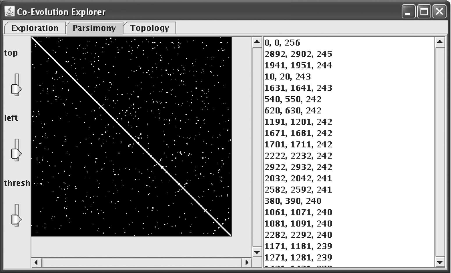
Screenshot of a Java implementation.

The algorithm has been tested on simulated data, as follows: In each experiment we generate a random binary tree with 20 leaves, and place a random DNA string (alphabet = {a, c, g, t}) of length 2000 on the root. Ten disjoint “domains” of length 12 are selected at random in this string, and a directed acyclic graph G is generated at random, having these ten domains as vertices, with arcs between two domains that are to coevolve in this simulation. (Seven was a typical number of arcs.) Next we repeatedly mutate the string from parent to child until each leaf has a string on it. (We have no insertions, deletions or rearrangements in this model of co-evolution.) For mutating we select two probabilities: p_in for mutating characters in domains and p_out for mutating characters which are not in any domain. If the i th character in the parent is not in any domain, then the ith character in the child's string will be the same with probability 1 − p_out, and each of the other three characters with probability p_out /3. If the ith character is in a domain, then we distinguish two cases: If the domain has no directed arc to another domain, then we mutate it just as we did for non-domain characters, but with probability p_in in place of p_out. If the domain has directed arcs to other domains, say D₁ … D_k, then we first recursively mutate those domains and afterward, look at what happened. For each D_i we compare the domain in the parent to the domain in the child, count the number c_i of changes (mutations) that occur, and let p_i = c_i /12 represent the observed probability of mutation inside the ith domain. Finally, we let P = min_i p_i, and mutate the characters inside this domain as we did for characters not in any domain, but using P in place of p_out. This has the effect of suppressing mutation in domains when mutation does not occur in domains with which they are co-evolving, and encouraging mutation when many mutations happen in their co-evolving partners. C++ source code for generating such test cases (but with commandline parameters to vary the constants mentioned above) is also freely available from the author.

When the correlation algorithm is run and highly correlated pairs of domains of length 12 were output, it was typical to find such things as domain S (100, 111) highly correlated with S (350, 361), and also highly correlated with regions S (351, 362) and S (352, 363). So we put in a post-processing clustering step so that, within each cluster, only the most highly-correlated pair of domains would be output.

Tests on the simulated data indicate that approximately one-third of co-evolving pairs are discovered by the correlation algorithm. We tested as follows: Once the digraph was generated, we knew how many co-evolving pairs we should expect to find. Then in the Java program, we set the threshold so that twice that many pairs would be presented to the user, and we counted a success if among them we found a pair of domains both of which overlapped at least 9 of the 12 characters of the domains in some pair that was present in our simulated data. For example, in one set of runs we generated five sets of data (each consisting of 20 strings of length 2000) using probability p_in = p_out = 1/10. Each had ten domains, the numbers of arcs in the diagraph were 7, 7, 8, 5, and 9, and the Java program found 3, 2, 2, 3, and 3 of the pairs, respectively. These results get worse once the value of p_in drops below approximately 1/20 (for domains of length 12) but don't change appreciably for larger values of p_in.

3.3. Contrast with “footprinting” and further uses

In phylogenetic footprinting, one searches for regions of the strings which have mutated less than the surrounding regions, and identify these conserved regions as potentially significant. With the algorithm herein proposed we can find regions whose mutation rate is the same as the background string, or, indeed, higher. What we're measuring is not the amount of change, but the relative rates of change across the phylogenetic tree. Where footprinting is looking for a single region with low elevation, we're looking for pairs of regions having similar terrain, regardless of elevation. Which raises the possibility of using this algorithm as a data mining technique, wherein one wishes to find features which individually may not stand out from the general population, but which can be discerned by virtue of their correlation to other, equally unnoticeable features.

Footnotes

Disclosure Statement

No competing financial interests exist.

References

Blanchette

2002. Algorithms for phylogenetic footprinting. J. Comput. Biol., 9, 211–224.

Fitch

W.M.

1971. Toward defining the course of evolution: minimum change for a specific tree topology. Syst. Zool., 20, 406–416.

Glazier

A.M.

, Nadeau

J.H.

, and Aitman

T.J.

2002. Finding genes that underlie complex traits. Science, 298, 2345–2349.

Jothi

, Kann

M.G.

, and Przytycka

T.M.

2005. Predicting protein-protein interaction by searching evolutionary tree automorphism space. Bioinformatics, 21, Suppl 1, 241–250.

Kim

, Koyutürk

, Topkara

, et al. 2006. Inferring functional information from domain co-evolution. Bioinformatics, 22, 40–49.

, Chen

, Huang

, et al. 2007. Global mapping of gene/protein interactions in pubmed abstracts: a framework and an experiment with p53 interactions. J. Biomed. Inform., 40, 453–464.

Ramani

A.K.

, and Marcotte

E.M.

2003. Exploiting the co-evolution of interacting proteins to discover interaction specificity. J. Mol. Biol., 327, 273–284.

Rinsma

, Hendy

, and Penny

1990. Minimally colored trees. Math. Biosci., 98, 201–210.

Tamayo

A.G.

, Bharti

, Trujillo

, et al. 2008. Copi coatomer complex proteins facilitate the translocation of anthrax lethal factor across vesicular membranes in vitro. Proc. Nat. Acad. Sci. U.S.A.

10.

Tukey

J.W.

1975. Mathematics and the picturing of data. Proc. Int. Congr. Math., 2, 523–531.