Phylogeny Inference Based on Spectral Graph Clustering

Abstract

Phylogeny inference is an importance issue in computational biology. Some early approaches based on characteristics such as the maximum parsimony algorithm and the maximum likelihood algorithm will become intractable when the number of taxonomic units is large. Recent algorithms based on distance data which adopt an agglomerative scheme are widely used for phylogeny inference. However, they have to recursively merge the nearest pair of taxa and estimate a distance matrix; this may enlarge the error gradually, and lead to an inaccurate tree topology. In this study, a splitting algorithm is proposed for phylogeny inference by using the spectral graph clustering (SGC) technique. The SGC algorithm splits graphs by using the maximum cut criterion and circumvents optimization problems through solving a generalized eigenvalue system. The promising features of the proposed algorithm are the following: (i) using a heuristic strategy for constructing phylogenies from certain distance functions, which are not even additive; (ii) distance matrices do not have to be estimated recursively; (iii) inferring a more accurate tree topology than that of the Neighbor-joining (NJ) algorithm on simulated datasets; and (iv) strongly supporting hypotheses induced by other methods for Baculovirus genomes. Our numerical experiments confirm that the SGC algorithm is efficient for phylogeny inference.

1. Introduction

Phylogeny inference is an important issue in computational biology. Phylogenetic tree can provide insight into the evolutionary relationships in taxonomic groups and the divergent time between different organisms. Over the past several decades, biologists, mathematicians, statisticians, and computer scientists have designed a variety of methods to reconstruct the phylogenetic tree. Algorithms for phylogeny inference can be generally classified into two groups: character-based and distance-based methods.

The character-based group includes three types of methods: (1) methods based on maximum parsimony; (2) methods based on maximum likelihood (ML); and (3) methods based on Bayesian inference. The maximum parsimony algorithm was first proposed by Camin and Sokal (1965), and extended by Hein (1990, 1993). It has been successfully used to investigate the evolution history of various genera for almost 30 years; however, it has been proved to be NP-hard (Foulds and Graham, 1982), which makes it impractical when the number of taxa become large. Basically, maximum parsimony–based algorithms examine all possible trees and select the one with the smallest number of evolutionary changes; in other words, maximum parsimony algorithms predict the evolutionary tree that minimizes the number of steps required to generate the observed variation in the sequences from the ancestral sequences. Maximum likelihood (ML)–based algorithms attempt to reconstruct a phylogeny by using an explicit model of evolution (Felsenstein, 1981; Jin et al., 2006; Keane et al., 2005); they have nice statistical properties and can always yield a proper result when an appropriate model is used. However, the ML methods have also been proved to be NP-hard (Chor and Tuller, 2005). Besides, the ML algorithms depend heavily on selected models. As a result, the ML algorithms make themselves difficult for practical use in many cases. Bayesian inference–based approaches employ the principle of maximum posterior probability, and have been successfully used in many application scenarios (Feng et al., 2003; Holder and Lewis, 2003; Huelsenbeck and Ronquist, 2001; Larget and Simon, 1999; Ninio et al., 2007; Yang and Rannala, 1997). However, as the prior distribution needs to be estimated, and many parameters should be integrated in this kind of methods, the Bayesian-based methods are also time-consuming in practice.

Approaches in the distance-based group are based on the principle of minimum evolution (ME) (Birin et al., 2008; Grünewald et al., 2007; Kumar, 1996; Rzhetsky and Nei, 2003), they reconstruct phylogenetic trees by using evolutionary distance data. The first algorithm of this kind was proposed by Kidd and Sgaramella-Zonta (1971) to search for the tree with the smallest sum of branch length. These algorithms examine all the possible topologies close to the true tree and choose the one that shows the smallest amount of total evolutionary change take place. However, this approach is intractable for a large dataset. In order to circumvent this problem, many heuristic algorithms based on an agglomerative scheme were proposed to calculate the phylogenetic tree. Most of these approaches start from a distance matrix, iteratively pick out a pair of taxa according to certain criterion, create a new node to represent them, and then reduce the distance matrix by replacing both taxa with this node. This procedure repeats until there are only three taxa left (Criscuolo and Gascuel, 2008; Evans et al., 2006; Gascuel, 1997; Howe et al., 2002; Mailund et al., 2006).

Neighbor-Joining (NJ) is the most popular and widely used agglomerative algorithm based on the principle of minimum evolution; it was introduced by Saitou and Nei (1987) and modified by Studier and Keppler (1988). Due to its greedy agglomerative scheme, NJ algorithm does not always find the ME tree, but instead a tree whose topology is similar to that of the ME tree (Saitou and Nei, 1986).

Although agglomerative approaches have been widely used for phylogeny inference (Criscuolo and Gascuel, 2008; Evans et al., 2006; Kumar and Gadagkar, 2000; Mailund et al., 2006; Rosenberg and Kumar, 2001; Takahashi and Nei, 2000), they have to estimate the evolutionary distance between pairwise nodes and reconstruct the distance matrix at each step; this makes the algorithm time consuming. Secondly, the error of distance value estimated at each step may be amplified along with the agglomerative procedure; these algorithms will not necessarily produce the most accurate tree topology. Besides, the agglomerative algorithms work from the local point of view, which can easily lead to a local optimal result.

In recent years, the split strategy has drawn more and more attention from the community of the phylogeny analysis. This kind of approach considers the phylogenetic tree reconstruction problem as a graph-cutting problem and adopts the maximum cut criterion to solve the graph-cutting problem, which has been well studied (Delorme and Poljak, 1993; Goemans and Williamson, 1995). The split strategy reconstructs the phylogenetic tree from a global point of view and has been successfully applied in phylogeny analysis. Snir and Rao (2006) adopted the max cut criterion in their supertree method to successfully reconstruct phylogenetic tree from triplet trees. Bansal and Bafna (2008) used max-cut criterion to solve the haplotype assembly problem.

The focus of this article is to adopt the splitting scheme to phylogeny inference. We proposed a spectral graph clustering (SGC) algorithm based on the spectral graph theory. A distance matrix characterizing the relationships among different species investigated was first constructed, each element in which denoted the evolutionary distance between two taxa. Then the spectral graph theory was applied to this matrix to solve the clustering problem by employing the partition strategy which adopted the maximum cut criterion. To this aim, the eigenvectors of the Laplacian Matrix derived from the distance matrix were calculated, and the one corresponding to the largest eigenvalue was selected as the candidate vector. Finally, the graph was split into two parts according to this eigenvector. This procedure was carried out recursively until all nodes of the trees contained only two leaves. The SGC algorithm produced more accurate tree topologies on simulated datasets than NJ algorithm, and supported hypotheses proposed by other methods on the Baculovirus genomes. Our method has the following advanced properties: (1) it is a useful heuristics for constructing phylogenies from certain distance functions, which are not even additive, and (2) the SGC algorithm can quickly reconstruct the phylogenetic tree by recursively splitting the graph with the time complexity of O(n³). It is a promising alternative to agglomerative methods.

2. Methods

2.1. Maximum cut–based spectral graph clustering

The clustering problem can be treated as a graph partitioning problem, and can be effectively addressed through a generalized eigenvalue system based on certain optimality criterion. Suppose we have a graph G = (V;E), where V denotes the node set and E the edge set. The elements in E represent the relationships among pairwise nodes. The relationships among the nodes can be rewritten by a matrix W, whose element w_ij represents the edge weight e_ij corresponding to node i and j (in this study, it denotes the evolutionary distance between species i and j). Now we are given a distance matrix. Our task is to divide the graph into disjoint parts so that the total dissimilarity between the different groups and the total similarity within the groups are both maximum.

In the bipartition scenario, the task of graph partitioning problem is to divide a set V into two parts: A and B, and they satisfy A ∪ B = V and A ∩ B = φ. Meanwhile, we hope the inter-class distance value between A and B is large, while the total intra-class distance value within them is as small as possible; this criterion is called maximum cut. Unfortunately, this problem is intractable when there are many nodes involved; it is NP-hard like the partition problem based on the normalized cut criterion (Garey and Johnson, 1979; Shi and Malik, 2000). Many approximate methods have been proposed to this problem; Delorme and Poljak (1993) gave an upper bound of nλ_max(L + U)/4 for it by using Laplacian eigenvalues. The well-known approximation algorithm for this problem was introduced by Goemans and Williamson (1995) with a 0.878 performance guarantee, which relaxed it to a semidefinite programming problem and adopted a randomized scheme to split the vertices. It is obvious that the randomly rounding scheme cannot always guarantee correct clustering. Mahajan and Ramesh (1999) later presented a derandomization scheme for approximation algorithms based on semidefinite programming; it is interesting from a purely theoretical point of view, but in practice this derandomization scheme is very complicated and has a huge running time (Andersson, 2000).

In this study, we adopted the spectral graph theory to this optimization problem. The integer quadratic program was first relaxed to an eigenvalue problem, and the relationships among vertices were preserved and embedded into a low-dimensional space by solving the eigenvalue system; then a simple deterministic scheme was adopted to efficiently split the vertices in the graph into different clusters based on the one-dimensional eigenvector. As will be shown, when we embed the maximum cut problem into the real value domain, an approximate discrete solution can be found efficiently.

Suppose that we have an indicator vector p with \documentclass{aastex}\usepackage{amsbsy}\usepackage{amsfonts}\usepackage{amssymb}\usepackage{bm}\usepackage{mathrsfs}\usepackage{pifont}\usepackage{stmaryrd}\usepackage{textcomp}\usepackage{portland,xspace}\usepackage{amsmath,amsxtra}\pagestyle{empty}\DeclareMathSizes{10}{9}{7}{6} \begin{document} \begin{align*} p_i = \left\{\begin{matrix}1 & p_i \in A \\ - 1 & p_i \in B\end{matrix} \right. \tag{1} \end{align*} \end{document}

Then we can define the maximum cut criterion as \documentclass{aastex}\usepackage{amsbsy}\usepackage{amsfonts}\usepackage{amssymb}\usepackage{bm}\usepackage{mathrsfs}\usepackage{pifont}\usepackage{stmaryrd}\usepackage{textcomp}\usepackage{portland,xspace}\usepackage{amsmath,amsxtra}\pagestyle{empty}\DeclareMathSizes{10}{9}{7}{6} \begin{document} \begin{align*} \max \{Cut (A,B) \} &= \max \left\{ \frac {1} {2} \sum_ {i,j \in V} w_ {ij} (p_i - p_j)^2 \right\} \\ &= \max \left\{ \frac {1} {2} \left[ \sum_{j \in V} \sum_{i \in V} w_{ij} \ p_i^2 + \sum_{i \in V} \sum_{j \in V} w_{ij} \ p_j^2 - 2 \sum_{i \in V} \sum_{j \in V} p_{i} w_{ij} \ p_j \right] \right\} \\ &= \max \left\{ \frac {1} {2} \left[ p^{T} Dp + p^{T} Dp - 2p^{T} Wp \right] \right\} \\ &= \max \left\{ p^{T} Dp - p^{T} Wp \right\} \\ &= \max \left\{ p^{T} Lp \right\} \tag {2} \end{align*} \end{document}

where w_ij ɛ W is the distance between node i and j, D is a diagonal matrix with D_ij = ∑_j w_ij and L = D − W is the Laplacian Matrix of W (Fieder, 1973).

As mentioned above, it is difficult to solve this optimization problem for discrete value p; here we relax p to continuous value and impose the equality constraint ||p|| = 1, and then the maximum optimization problem can be solved by introducing the Lagrange undeter-mined multipliers as follows, \documentclass{aastex}\usepackage{amsbsy}\usepackage{amsfonts}\usepackage{amssymb}\usepackage{bm}\usepackage{mathrsfs}\usepackage{pifont}\usepackage{stmaryrd}\usepackage{textcomp}\usepackage{portland,xspace}\usepackage{amsmath,amsxtra}\pagestyle{empty}\DeclareMathSizes{10}{9}{7}{6} \begin{document} \begin{align*} f (p) = p^T Lp - \lambda (p^T p - 1) \tag{3} \end{align*} \end{document}

Computing the partial derivative of f with respect to p and we get \documentclass{aastex}\usepackage{amsbsy}\usepackage{amsfonts}\usepackage{amssymb}\usepackage{bm}\usepackage{mathrsfs}\usepackage{pifont}\usepackage{stmaryrd}\usepackage{textcomp}\usepackage{portland,xspace}\usepackage{amsmath,amsxtra}\pagestyle{empty}\DeclareMathSizes{10}{9}{7}{6} \begin{document} \begin{align*} \frac {\partial f} {\partial p} = 2Lp - 2 \lambda p \tag {4} \end{align*} \end{document}

Setting the derivative of the above equation to be zero, we have that Lp − λp = 0, i.e., Lp = λp, Especially, we have \documentclass{aastex}\usepackage{amsbsy}\usepackage{amsfonts}\usepackage{amssymb}\usepackage{bm}\usepackage{mathrsfs}\usepackage{pifont}\usepackage{stmaryrd}\usepackage{textcomp}\usepackage{portland,xspace}\usepackage{amsmath,amsxtra}\pagestyle{empty}\DeclareMathSizes{10}{9}{7}{6} \begin{document} \begin{align*} p^T Lp = p^T \lambda p = p^T p \lambda, \tag{5} \end{align*} \end{document}

So, the following holds: \documentclass{aastex}\usepackage{amsbsy}\usepackage{amsfonts}\usepackage{amssymb}\usepackage{bm}\usepackage{mathrsfs}\usepackage{pifont}\usepackage{stmaryrd}\usepackage{textcomp}\usepackage{portland,xspace}\usepackage{amsmath,amsxtra}\pagestyle{empty}\DeclareMathSizes{10}{9}{7}{6} \begin{document} \begin{align*} \frac {p^T Lp} {p^T p} = \lambda, \tag {6} \end{align*} \end{document}

According to the constraint p^T p = ||p|| = 1, the optimal problem becomes \documentclass{aastex}\usepackage{amsbsy}\usepackage{amsfonts}\usepackage{amssymb}\usepackage{bm}\usepackage{mathrsfs}\usepackage{pifont}\usepackage{stmaryrd}\usepackage{textcomp}\usepackage{portland,xspace}\usepackage{amsmath,amsxtra}\pagestyle{empty}\DeclareMathSizes{10}{9}{7}{6} \begin{document} \begin{align*} \max (p^T Lp) = \max \left(\frac {p^T Lp} {p^T p} \right) \tag {7} \end{align*} \end{document}

As L is a positive semi-definite matrix (Chung, 1997), according to the Rayleigh Quotient Theorem (Golub and Van Loan, 1989) when we relax the indicators in p from discrete value to continuous value, the cut value max{Ncut(A,B)} can be maximized by solving the following generalized eigenvalue system when p is the eigenvector corresponding to the largest eigenvalue: \documentclass{aastex}\usepackage{amsbsy}\usepackage{amsfonts}\usepackage{amssymb}\usepackage{bm}\usepackage{mathrsfs}\usepackage{pifont}\usepackage{stmaryrd}\usepackage{textcomp}\usepackage{portland,xspace}\usepackage{amsmath,amsxtra}\pagestyle{empty}\DeclareMathSizes{10}{9}{7}{6} \begin{document} \begin{align*} Lp = \lambda p \tag{8} \end{align*} \end{document}

Thus, the graph partition problem is connected with the generalized eigenvector of the Laplacian Matrix of the distance matrix of the graph. The largest eigenvector of the Laplacian matrix is the real value solution to the bipartition problem based on the maximum cut criterion. This vector contains the structural information of the graph and can be used to divide the graph into two parts by means of simple clustering algorithm. Thus, the graph partition problem can be solved by spectral clustering approach, while the phylogenetic tree can be reconstructed by performing the spectral clustering algorithm recursively. In this study, the elements in the vector were sorted and split into two clusters where the gap was the maximum, each of which corresponded to a subgroup of species. The procedure of our approach is shown next, and the SGC algorithm is shown in Figure 1:

Compute the distance matrix, which denotes the pairwise evolutionary distance.

Solve the eigenvalue system Lp = λp, and select an eigenvector corresponding to the largest eigenvalue.

Sort the eigenvector, and divide it into two subsets at the position where the gap between two adjacent elements is the largest.

Go to (a) to recursively split the subsets obtained from (c) until they contain no more than two elements.

FIG. 1.

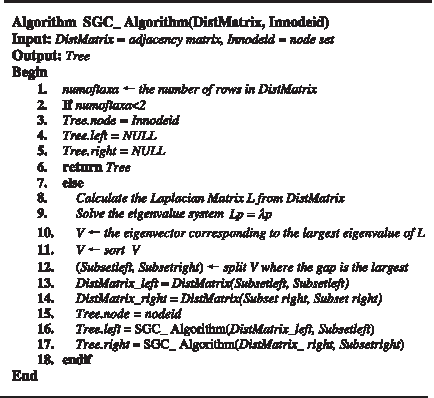
The spectral graph clustering (SGC) algorithm.

Step (b) is the most time consuming in this procedure; it needs O(n²) time complexity to solve the eigenvalue system. Steps (b) and (c) should be repeated n − 1 times, so the SGC algorithm has O(n³) time complexity, where n is the number of taxa involved.

2.2. Datasets

2.2.1. Simulated datasets

Three simulated datasets were generated and used to validate our algorithm. Each of them contains 100 groups, and each group included 100 genome sequences, which were evolved from one into another step by step; i.e., the second sequence was evolved from the original one, the third sequence was from the second one, and so on. Each dataset was generated by the mutation operators related to one kind of the following mutation information: gene gain or loss, gene rearrangement, and gene local mutation (point mutation). The gene gain or loss information is related to operators such as gene replication, gene insertion and gene deletion, the gene rearrangement involved gene reversion, gene transposition, gene reversal and gene transposition, while the gene local mutation is relevant with three kinds of operators: base insertion, base deletion, and base substitution. In a mutation step, the number of genes involved with gene gain or loss was randomly fallen into the interval [1, 5]; the genes relevant to gene rearrangement operator occupied 10% of the total number of the genes in the complete genome sequence; as for the local mutation, the mutation rate was 10% for the 10% of genes randomly selected from the complete genome. One mutation step was defined as the mutation that evolved one genome sequence into another, e.g., from the original genome sequence into the second one in a group of dataset.

In order to reduce the computational complexity and see whether the mutation distance has effects on the tree topologies, we sampled three subsets from every dataset; each subset contained 100 genera, and each genus included 10 genomes. The first subset's sampling interval (SI) was one; i.e., the 10 genomes were selected from the dataset in the same order as they evolved, every pair of adjacent sequences was involved with only one mutation step, and the first genome was randomly select from the top ninety genomes. The second data subset had SI of five, i.e., every two successive genomes in the subset was involved with five evolutionary steps. The third data subset had SI of 10. Thus, we had nine simulated subsets: three were relevant to gene gain and loss, three were involved with gene rearrangement, and the rest were evolved by local mutation operators.

2.2.2. Real datasets

The real dataset contained 29 complete genomes of Baculovirus obtained from NCBI: Adoxophyes orana granulovirus (AdorGV AF547984), Cryptophlebia leucotreta granulovirus (CrleGV AY229987), Cydia pomonella granulovirus (CpGV U53466), Phthorimaea operculella granulovirus (PhopGV AF499596), Plutella xylostella granulovirus (PlxyGV AF270937), Xestia c-nigrum granulovirus (XecnGV AF162221), Agrotis segetum granulovirus (AgseGV AY522332), Spodoptera litura granulovirus (SpltNPV DQ288858), Adoxophyes honmai NPV (AdhoNPV AP006270), Achiplusia ou MNPV (RoMNPV AY145471), Bombyx mori NPV (BmNPV L33180), Choristoneura fumiferana DEF MNPV (CfDEFNPV AY327402), Choristoneura fumiferana MNPV (CfMNPV AF512031), Culex nigrip-alpus NPV (CuniNPV AF403738), Epiphyas postvittana NPV (EppoNPV AY043265), Helicoverpa armigera NPV (HearNPV_C1 AF303045), Helicoverpa zea (HzSNPV AF334030), Lymantria dispar MNPV (LdMNPV AF081810), Mamestra configurata NPV-A (MacoNPV U59461), Mamestra configurata NPV-B (MacoNPV_B AY126275), Neodiprion lecontii NPV (NeleNPV AY349019), Neodiprion sertifer NPV (NeseNPV AY430810), Orgyia pseudotsugata MNPV (OpMNPV U75930), Spodoptera exigua MNPV (SeMNPV AF169823), Spodoptera litura NPV (SpltNPV AF325155), Trichoplusia ni SNPV (TnSNPV DQ017380), Agrotis segetum nucleopolyhedrovirus (AgseNPV DQ123841), Autographa californica nucleopolyhedrovirus (AcMNPV L22858), Chrysodeixis chalcites nucleopolyhedrovirus (ChchNPV AY864330), and Helicoverpa armigera nucleopolyhedrovirus G4 (HearNPV_G4 AF271059).

2.3. Distance function used to compute the adjacent matrix

In this study, three kinds of distance metric were used to compute the distance matrix:

Distance based on gene content (Snel et al., 1999). Gene content is the fraction of genes two genomes have in common (named as common gene), which was used to characterize the evolutionary distance relevant to the gene gain and gene loss events. This kind of distance was conventionally defined as \documentclass{aastex}\usepackage{amsbsy}\usepackage{amsfonts}\usepackage{amssymb}\usepackage{bm}\usepackage{mathrsfs}\usepackage{pifont}\usepackage{stmaryrd}\usepackage{textcomp}\usepackage{portland,xspace}\usepackage{amsmath,amsxtra}\pagestyle{empty}\DeclareMathSizes{10}{9}{7}{6} \begin{document} \begin{align*} D \_\, content_ {AB} = 1 - \frac {\mid C \mid} {\min (\mid A \mid, \mid B \mid)} \tag {9} \end{align*} \end{document}

where |C| is the number of elements in set C, |A| and |B| are the numbers of genes in genome A and B, respectively.

Distance based on mean identity. Sequence identity is the fraction of identical bases that two genes have. If the identities of all the common genes are taken into account, a new measure can be defined to characterize the local evolutionary event on the complete genome sequences, and the evolutionary distance based on the identities of all the common genes can be computed as follows: \documentclass{aastex}\usepackage{amsbsy}\usepackage{amsfonts}\usepackage{amssymb}\usepackage{bm}\usepackage{mathrsfs}\usepackage{pifont}\usepackage{stmaryrd}\usepackage{textcomp}\usepackage{portland,xspace}\usepackage{amsmath,amsxtra}\pagestyle{empty}\DeclareMathSizes{10}{9}{7}{6} \begin{document} \begin{align*} D \_\, identity_ {AB} = 1 - \frac {1} {\mid C \mid} \sum_ {i \in C} identity (i) \tag {10} \end{align*} \end{document}

where identity(i) is the identity value of the ith pairwise common genes, and |C| is the number of common genes.

Breakpoint distance. The breakpoint distance reflects the disruption of gene order, which was introduced early into computational studies (Nadeau and Taylor, 1984). Taking two adjacent genes g₁ and g₂ in genome A, we consider that a breakpoint has occurred when they do not appear consecutively in genome B as either the pair (g₁ g₂) or (−g₂−g₁). All the breakpoints between two genomes are counted, and the breakpoint distance can be defined as \documentclass{aastex}\usepackage{amsbsy}\usepackage{amsfonts}\usepackage{amssymb}\usepackage{bm}\usepackage{mathrsfs}\usepackage{pifont}\usepackage{stmaryrd}\usepackage{textcomp}\usepackage{portland,xspace}\usepackage{amsmath,amsxtra}\pagestyle{empty}\DeclareMathSizes{10}{9}{7}{6} \begin{document} \begin{align*} D \_\, breakpoint_ {AB} = \frac {NumofBreakpo {\rm int}} {\mid C \mid} \tag {11} \end{align*} \end{document}

where |C| is the number of common genes.

2.4. Topological accuracy measure

In this study, two measures have been used to assess the accuracy of tree reconstruction, the most commonly used Robinson-Foulds (RF) measure (Robinson and Foulds, 1981) and the Percentage of Correct tree (PC). The RF distance between two trees is the number of bipartitions that differentiate between them. It is defined as follows.

Let T be a tree “leaf labeled” by a set S of taxa, an edge e = (u,v) in T defines a bipartition π_e on the leaves (induced by the deletion of e), which divides S into two sets, the set of all leaves on one side of the edge, and the set of all other leaves, so that we can define the set C(T) = {Π_e : e ɛ E(T)}, where E(T) is the set of all internal edges of T. If T is a model tree and T′ is the tree inferred by a phylogenetic reconstruction method, we define the false positives to be the edges of the set C(T′) − C(T) and the false negatives to be those of the set C(T) − C(T′), \documentclass{aastex}\usepackage{amsbsy}\usepackage{amsfonts}\usepackage{amssymb}\usepackage{bm}\usepackage{mathrsfs}\usepackage{pifont}\usepackage{stmaryrd}\usepackage{textcomp}\usepackage{portland,xspace}\usepackage{amsmath,amsxtra}\pagestyle{empty}\DeclareMathSizes{10}{9}{7}{6} \begin{document} \begin{align*} FPR = \mid C (T^{\prime}) - C (T) \mid / (n - 3) \tag {12} \end{align*} \end{document} \documentclass{aastex}\usepackage{amsbsy}\usepackage{amsfonts}\usepackage{amssymb}\usepackage{bm}\usepackage{mathrsfs}\usepackage{pifont}\usepackage{stmaryrd}\usepackage{textcomp}\usepackage{portland,xspace}\usepackage{amsmath,amsxtra}\pagestyle{empty}\DeclareMathSizes{10}{9}{7}{6} \begin{document} \begin{align*} FNR = \mid C (T) - C (T^{\prime}) \mid / (n - 3) \tag {13} \end{align*} \end{document}

When both trees are binary with the number of taxa N, we have FPR = FNR and N−3 internal edges in a binary tree, the false positive and false negative rates are values in the range [0, 1]. The RF distance between T and T′ is simply the average of these two rates, \documentclass{aastex}\usepackage{amsbsy}\usepackage{amsfonts}\usepackage{amssymb}\usepackage{bm}\usepackage{mathrsfs}\usepackage{pifont}\usepackage{stmaryrd}\usepackage{textcomp}\usepackage{portland,xspace}\usepackage{amsmath,amsxtra}\pagestyle{empty}\DeclareMathSizes{10}{9}{7}{6} \begin{document} \begin{align*} RF (T, T^ {\prime}) & = \frac {FPR + FNR} {2} \\ & = \frac {\mid C (T^ {\prime}) - C (T) \mid + \mid C (T) - C (T^ {\prime}) \mid} {2 (N - 3)} & (14) \end{align*} \end{document}

RF distance value of 1 implies that two trees have no bipartitions in common, while the value 0 means the identical topology of trees.

The fitness of an inferred tree can be defined as \documentclass{aastex}\usepackage{amsbsy}\usepackage{amsfonts}\usepackage{amssymb}\usepackage{bm}\usepackage{mathrsfs}\usepackage{pifont}\usepackage{stmaryrd}\usepackage{textcomp}\usepackage{portland,xspace}\usepackage{amsmath,amsxtra}\pagestyle{empty}\DeclareMathSizes{10}{9}{7}{6} \begin{document} \begin{align*} Fit \_tree = \begin{cases}1 \quad RF (T, T^{\prime}) = 0 \\ 0 \qquad otherwise\end{cases} \tag{15} \end{align*} \end{document}

Then the PC can be computed as \documentclass{aastex}\usepackage{amsbsy}\usepackage{amsfonts}\usepackage{amssymb}\usepackage{bm}\usepackage{mathrsfs}\usepackage{pifont}\usepackage{stmaryrd}\usepackage{textcomp}\usepackage{portland,xspace}\usepackage{amsmath,amsxtra}\pagestyle{empty}\DeclareMathSizes{10}{9}{7}{6} \begin{document} \begin{align*} PC = 100 {\times} \frac {1} {n} {\times} \sum_ {k = 1} ^n Fit \_ tree (k) \tag {16} \end{align*} \end{document}

where n is the number of trees in a data set.

3. Results and Discussion

3.1. Results on simulation datasets

The three kinds of distance metric mentioned above were used to compute the adjacent matrices, each of which represented the evolutionary relationships among a family of genomes corresponding to one category of evolutionary events. Then both SGC and the widely used NJ algorithm were applied to these distance matrices, and the inferred trees were compared with the model trees; the RF distance and the PC were calculated for every subset (one subset contained one hundred families of genomes with the same SI). The experimental results of our method and NJ algorithm on different data sets are listed in Table 1. As shown in this table, the SGC algorithm got better results for PC and less average RF distance than NJ algorithm for most of the SIs in all evolutionary scenarios, the PC values of SGC algorithm were always larger than that of NJ algorithm, and the average RF values were always smaller. The PC and average RF values of the both algorithm changed in the same way with the increase of SI under the three scenarios of gene local mutation, namely, the PC value increased with the growth of SI, while the average RF value declined with the growth of SI. It meant that lager mutation distance could always induce better phylogenetic tree. Comparing with gene rearrangement and gene local mutation, the scenarios related to gene gain and loss had faster growth of PC value, which grew from 45% to 75% as SI rose from 1 to 10, while the RF distance had an opposite changing direction under such condition.

Table 1.

Comparison of Simulated Datasets Produced by SGC and NJ Algorithm

	SGC		NJ
SI	PC (%)	Average RF distance	PC (%)	Average RF distance
Local mutation
1	48	0.135	3	0.276
5	51	0.126	4	0.285
10	54	0.102	5	0.242
Gene rearrangement
1	66	0.063	61	0.086
5	68	0.057	67	0.061
10	71	0.053	69	0.055
Gene gain and loss
1	45	0.125	42	0.152
5	73	0.057	70	0.061
10	75	0.048	75	0.046

The larger Sampling Interval (SI) means lager evolutionary distance. Percentage of Correct tree (PC) is the percentage of trees whose Robinson-Foulds (RF) distance equal to zero, the larger PC value means more trees' topologies are correctly inferred. The average RF distance is the average value of distance between the inferred tree and the model tree; the smaller average RF value means more reasonable local topological structure in the phylogenetic trees. NJ, Neighbor Joining; SGC, Spectral Graph Clustering.

Comparing with the other two kinds of evolutionary scenarios, the gene local mutation scenario produced the poorest results by the both algorithms. It is notable that the PC values of our method were significantly lager than that of the NJ method, with about 50% higher in average, while our average RF values were much smaller, with an average decline of 0.15. This might be caused by the very small distance values in the distance matrix, since there were only 10% positions of the 10% genes involved with the gene local mutation in this study. The results imply that the SGC algorithm can produce a more accurate tree even though the distance value is small.

3.2. Results on real datasets

To illustrate the performance of SGC algorithm in real scenarios, we investigated a data set of Baculovirus genomes, which was studied by Herniou and colleagues (Herniou and Jehle, 2007; Herniou et al., 2001, 2003). Three experiments were carried out on three data subsets selected from this data set, and the phylogenetic trees inferred were compared with those built by other approaches.

The first real data subset contained nine Baculovirus genomes that were previously investigated by Herniou et al. (2001). Both SGC and NJ algorithms were applied to the adjacent matrix based on breakpoint distance derived from this data set, and the corresponding phylogenetic trees are demonstrated in Figure 2. The topology indicated that this family could be clearly classified into two clusters: nucleopolyhedrovirus (NPV) and granulovirus (GV), and NPV could be further divided into two subclasses: group I NPVs and group II NPVs (Fig. 2). Our result was consistent with Herniou's NJ tree based on the breakpoint distance of the 63 common genes (Herniou et al., 2001).

FIG. 2.

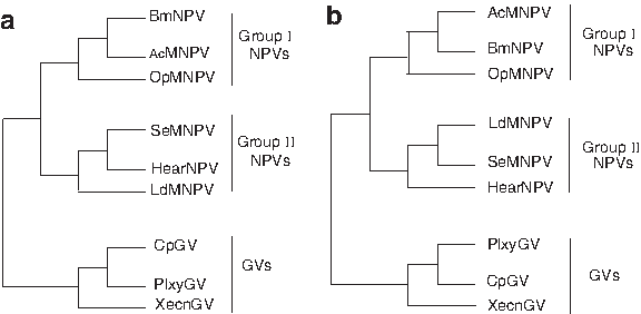
Gene order phylogenies for nine Baculovirus genomes. (a) Spectral clustering tree based on breakpoint distance. (b) Neighbor-joining tree based on breakpoint distance.

The second experiment was carried out on a data subset of 12 Baculovirus genomes investigated by Herniou et al. (2003). The gene content–based distance was derived from this dataset, and the tree inferred by our method as well as the NJ algorithm is shown in Figure 3. The two approaches both clearly split the family into two classes, i.e., NPV and GV, and then further divided NPV subfamily into two subsets: group I NPVs and group II NPVs. However, the topologies of group II NPVs were different; a possible reason is that the evolutionary relationship in this groups is still not clear.

FIG. 3.

Gene content phylogenies for 12 Baculovirus genomes. (a) Spectral clustering tree based on gene content distance. (b) Neighbor-joining tree based on gene content distance.

In the third experiment on real dataset, the distance matrix relevant to local mutation information of 29 Baculovirus genomes was used for phylogeny inference. The trees reconstructed by our method and by NJ algorithm had all the same topology (Fig. 4a, which was built by SGC algorithm). The tree inferred by Herniou's maximum likelihood method based on the distance matrix derived from the concatenated amino acid alignment of 29 core genes (Herniou and Jehle, 2007) is also shown in Figure 4b. According to the topology, our approach well supported three hypotheses of previous research based on gene phylogenies (Herniou and Jehle, 2007; Herniou et al., 2001, 2003; Lauzon et al., 2004) and complete genome analyses (Goodman et al., 2007; Lange et al., 2004; Zanotto et al., 1993):

FIG. 4.

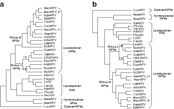
Baculovirus genome phylogenies for 29 Baculovirus genomes. (a) Spectral clustering tree based on mean identity of common genes. (b) Neighbor-joining tree based on the concatenated amino acid alignment of the 29 core baculovirus genes.

The Baculovirus contained four distinct families: Dipteran-specific NPVs, Hymenopteran-specific NPVs, Lepidopteran-specific GVs islated from Tortricidae, and Lepidopteran-specific NPVs. This also supported Rohrmann's result derived from the N-terminus of purified occlusion body protein (Rohrmann, 1986).

The Lepidopteran-specific NPVs included two subfamilies, group I and group II NPVs; those utilized different envelope fusion proteins for cell-to-cell spread. This was consistent with the phylogeny derived from the polh gene (Zanotto et al., 1993).

Group I NPVs could be further split into two clades, i.e., Ia (AcMNPV, RoMNPV, BmNPV) and Ib (OpMNPV, CfMNPV, CfDEFNPV, EppoNPV), which was consistent with the definition given by Jehle et al. (2006).

Our topology was also highly consistent with Herniou's maximum likelihood tree, except for the group II NPVs and GVs, whose intragroup relationships are still not very clear.

4. Conclusion

A novel algorithm (SGC algorithm) for phylogeny inference based on the splitting scheme was proposed from a global point of view. It employed spectral graph theory to solve the clustering problem and obtained the phylogeny of taxa investigated. The SGC algorithm produced more accurate tree topology on simulated datasets than NJ algorithm, especially in small mutation scenarios. Moreover, it supported the previous hypotheses proposed by other methods on the Baculovirus genomes. Our algorithm has O(n³) time complexity; it is a useful heuristic for constructing phylogenies from certain distance functions, which are not even additive. The SGC algorithm is a promising alternative to agglomerative methods.

Footnotes

Acknowledgments

We thank the anonymous referees who gave very helpful comments on the manuscript. This work was supported in part by the National Natural Sciences Foundation of China (grants 60675016 and 60633030).

Disclosure Statement

The authors declare that they have no competing interests.

References

Andersson

2000. Some new randomized approximation algorithms [Ph.D. disseration] Department of Numerical Analysis and Computer Science, Royal Institute of Technology: Stockholm.

Bansal

, Bafna

2008. HapCUT: an efficient and accurate algorithm for the haplotype assembly problem. Bioinformatics, 24:i153–i159.

Birin

, Gal-Or

, Elias

et al. 2008. Inferring horizontal transfers in the presence of rearrangements by the minimum evolution criterion. Bioinformatics, 24:826–832.

Camin

, Sokal

1965. A method for deducing branching sequences in phylogeny. Evolution, 19:311–326.

Chor

, Tuller

2005. Maximum likelihood of evolutionary trees: hardness and approximation. Bioinformatics, 21:97–106.

Chung

F.R.

1997. Spectral Graph Theory. American Mathematical Society: Providence, RI.

Criscuolo

, Gascuel

2008. Fast NJ-like algorithms to deal with incomplete distance matrices. BMC Bioinformatics, 9:166.

Delorme

, Poljak

1993. Laplacian eigenvalues and the maximum cut problem. Math. Programm., 62:557–574.

Evans

, Sheneman

, Foster

2006. Relaxed neighbor joining: a fast distance-based phylogenetic tree construction method. J. Mol. Evol., 62:785–792.

10.

Felsenstein

1981. Evolutionary trees from DNA sequences: a maximum likelihood approach. J. Mol. Evol., 17:368–376.

11.

Feng

, Buell

D.A.

, Rose

J.R.

et al. 2003. Parallel algorithms for Bayesian phylogenetic inference. J. Parallel Distr. Com., 63:707–718.

12.

Fieder

1973. Algebraic connectivity of graphs. Czech. Math. J., 22:298–305.

13.

Foulds

L.R.

, Graham

R.L.

1982. The steiner tree problem in phylogeny is np-complete. Adv. Appl. Math., 3:4–49.

14.

Garey

M.R.

, Johnson

D.S.

1979. Computers and Intractability: A Guide to the Theory of NP-Completeness. W.H. Freeman and Company: New York.

15.

Gascuel

1997. BIONJ: an improved version of the NJ algorithm based on a simple model of sequence data. Mol. Biol. Evol., 14:685–695.

16.

Goemans

M.X.

, Williamson

D.P.

1995. Improved approximation algorithms for maximum cut and satisfiability problems using semidefinite programming. J. ACM, 42:1145.

17.

Golub

G.H.

, Van Loan

C.F.

1989. Matrix Computations. Johns Hopkins Press: Baltimore.

18.

Goodman

, Ollikainen

, Sholley

2007. Baculovirus phylogeny based on genome rearrangements. Lect. Notes Comput. Sci., 4751:69–82.

19.

Grünewald

, Forslund

, Dress

A.W.

et al. 2007. QNet: An agglomerative method for the construction of phylogenetic networks from weighted quartets. Mol. Biol. Evol., 24:532–538.

20.

Hein

1990. Reconstructing evolution of sequences subject to recombination using parsimony. Math. Biosci., 98:185–200.

21.

Hein

1993. A heuristic method to reconstruct the history of sequences subject to recombination. J. Mol. Evol., 36:396–405.

22.

Herniou

E.A.

, Jehle

J.A.

2007. Baculovirus phylogeny and evolution. Curr. Drug Targets, 8:1043–1050.

23.

Herniou

E.A.

, Luque

, Chen

et al. 2001. Use of whole genome sequence data to infer baculovirus phylogeny. J. Virol., 75:8117–8126.

24.

Herniou

E.A.

, Olszewski

J.A.

, Cory

J.S.

et al. 2003. The genome sequence and evolution of baculoviruses. Annu. Rev. Entomol., 48:211–234.

25.

Holder

, Lewis

2003. Phylogeny estimation: traditional and Bayesian approaches. Nat. Rev. Genet., 4:275–284.

26.

Howe

, Bateman

, Durbin

2002. QuickTree: building huge neighbor-joining trees of protein sequences. Bioinformatics, 18:1546–1547.

27.

Huelsenbeck

J.P.

, Ronquist

2001. MRBAYES: Bayesian inference of phylogenetic trees. Bioinformatics, 17:754–755.

28.

Jehle

J.A.

, Lange

, Wang

H.L.

et al. 2006. Molecular identification and phylogenetic analysis of baculoviruses from Lepidoptera virology. Virology, 346:180–193.

29.

Jin

, Nakhleh

, Snir

et al. 2006. Maximum likelihood of phylogenetic networks. Bioinformatics, 22:2604–2611.

30.

Keane

T.M.

, Naughton

T.J.

, Travers

S.A.

et al. 2005. DPRml: distributed phylogeny reconstruction by maximum likelihood. Bioinformatics, 21:969–974.

31.

Kidd

K.K.

, Sgaramella-Zonta

L.A.

1971. Phylogenetic analysis: concepts and methods. Am. J. Hum. Genet., 23:235–252.

32.

Kumar

1996. A stepwise algorithm for finding minimum evolution trees. Mol. Biol. Evol., 13:584–593.

33.

Kumar

, Gadagkar

S.R.

2000. Efficiency of the neighbor-joining method in reconstructing deep and shallow evolutionary relationship in large phylogenies. J. Mol. Evol., 51:544–553.

34.

Lange

, Wang

H.L.

, Zhihong

et al. 2004. Towards a molecular identification and classification system of lepidopteran-specific baculoviruses. Virology, 325:36–47.

35.

Larget

, Simon

1999. Markov chain Monte Carlo algorithms for the Bayesian analysis of phylogenetic trees. Mol. Biol. Evol., 16:750–759.

36.

Lauzon

H.A.M.

, Lucarotti

C.J.

, Krell

P.J.

et al. 2004. Sequence and organization of the Neodiprion lecontei nucleopolyhedrovirus genome. J. Virol., 78:7023–7035.

37.

Mahajan

, Ramesh

1999. Derandomizing approximation algorithms based on semidefinite programming. SIAM J. Comput., 28:1641–1663.

38.

Mailund

, Brodal

G.S.

, Fagerberg

et al. 2006. Recrafting the neighbor-joining method. BMC Bioinformatics, 7:29.

39.

Nadeau

J.H.

, Taylor

B.A.

1984. Lengths of chromosomal segments conserved since divergence of man and mouse. Proc. Natl. Acad. Sci. USA, 81:814–818.

40.

Ninio

, Privman

, Pupko

et al. 2007. Phylogeny reconstruction: increasing the accuracy of pairwise distance estimation using Bayesian inference of evolutionary rates. Bioinformatics, 23:e136–e141.

41.

Robinson

D.F.

, Foulds

L.R.

1981. Comparison of phylogenetic trees. Math. Biosci., 53:131–147.

42.

Rohrmann

G.F.

1986. Polyhedrin structure. J. Gen. Virol., 67:1499–1513.

43.

Rosenberg

M.S.

, Kumar

2001. Traditional phylogenetic reconstruction methods reconstruct shallow and deep evolutionary relationship equally well. Mol. Biol. Evol., 18:1823–1827.

44.

Rzhetsky

, Nei

2003. Theoretical foundation of the minimum-evolution method of phylogenetic inference. Mol. Biol. Evol., 10:1073–1095.

45.

Saitou

, Nei

1986. The number of nucleotides required to determine the branching order of three species with special reference to the human-chimpanzee-gorilla divergence. J. Mol. Evol., 24:189–204.

46.

Saitou

, Nei

1987. The neighbor-joining method: a new method for reconstructing phylogenetic trees. Mol. Biol. Evol., 4:406–425.

47.

Shi

, Malik

2000. Normalized cuts and image segmentation. IEEE Trans. Pattern Anal., 22:888–905.

48.

Snel

, Bork

, Huynen

M.A.

1999. Genome phylogeny based on gene content. Nat. Genet., 21:108–110.

49.

Snir

, Rao

2006. Using max cut to enhance rooted trees consistency. IEEE/ACM Trans. Comput. Biol. Bioinform., 3:323–333.

50.

Studier

J.A.

, Keppler

K.J.

1988. A note on the neighbor-joining algorithm of Saitou and Nei, The neighbor-joining method: a new method for reconstructing phylogenetic trees. Mol. Biol. Evol., 5:729–731.

51.

Takahashi

, Nei

2000. Efficiencies of fast algorithms of phylogenetic inference under the criteria of maximum parsimony, minimum evolution, and maximum likelihood when a large number of sequences are used. Mol. Biol. Evol., 17:1251–1258.

52.

Yang

Z.H.

, Rannala

1997. Bayesian phylogenetic inference using DNA sequences: a Markov chain Monte Carlo method. Mol. Biol. Evol., 14:717–724.

53.

Zanotto

P.M.

, Kessing

B.D.

, Maruniak

J.E.

1993. Phylogenetic interrelationships among baculoviruses: evolutionary rates and host associations. J. Invertebr. Pathol., 62:147–164.