Haplotype Inference by Pure Parsimony: A Survey

1. Introduction

Haplotype inference is one of the most challenging problems in human genetics. The identification of haplotypes, which contain the genetic data inherited from each parent, may bring new insights into the genetic predisposition to disease, as well as the response to drugs.

Although a number of heritable disorders depend only on a single location in one single gene, common diseases usually depend on the combined effects of many different factors, in a number of different genes.

Current genotyping methods do not provide haplotype information. Instead, only genotypes, which correspond to the conflated data of haplotypes inherited from both parents, are provided. Although a number of association studies can be done using only genotypes, haplotype information is essential for the detailed analysis of the mechanisms of disease.

The identification of haplotypes makes it possible to perform haplotype-based association tests with diseases. This is particularly important on genome-wide association studies. Actually, haplotypic association studies have found loci associated with diseases that are not genome-wide significant using single-marker tests (Browning and Browning, 2008). Moreover, most imputation methods require the haplotypic data rather than genotypes.

The HapMap project ¹ (The International HapMap Consortium, 2003, 2005, 2007) represents a significant effort to develop a public resource that will help researchers to find genes associated with diseases. The HapMap project aims at making available genotype and haplotype information of a large and diversified sample of the human population.

Considering the huge amount of data to deal with and the intrinsic complexity of the problem, haplotype inference also poses a number of computational challenges. This is true regardless of the approach followed to infer the haplotypes.

One of the existing approaches for solving the haplotype inference problem is pure parsimony (Gusfield, 2003). Given that a solution has to be parsimonious, the original problem becomes a minimization problem. The first tools developed for solving the Haplotype Inference by Pure Parsimony (HIPP) problem were based on Integer Linear Programming (ILP), including exponential (Gusfield, 2003) and polynomial size models (Brown and Harrower, 2004, 2006; Halldórsson et al., 2004; Lancia et al., 2004; Bertolazzi et al., 2008), and branch-and-bound algorithms (Wang and Xu, 2003). More recently, new tools based on Boolean constraint solving, namely Boolean Satisfiability (SAT), Pseudo-Boolean Optimization (PBO), and Answer Set Programming (ASP), have been developed (Lynce and Marques-Silva, 2006; Graça et al., 2007; Erdem and Türe, 2008). The SAT/PBO/ASP-based tools use polynomial-size models and additional techniques for further reducing the size of the model. While the former HIPP tools could only solve small-size illustrative problem instances, the latter are remarkably more efficient, and capable of solving much larger and harder problem instances.

The recent algorithmic developments for solving the HIPP problem have made the pure parsimony approach competitive to the point that it can be considered an effective alternative to other more standard approaches. Not surprisingly, there is no clear best approach (i.e., different problem instances are solved differently by different approaches). The accuracy of each method depends on characteristics of the DNA region, in particular, on the level of selection and recombination in the region. However, there is still a comprehensive evaluation to be done in order to characterize the positive/negative aspects of each approach. One potential advantage of HIPP is result reproducibility. This is in contrast with statistical methods, which are unable to ensure reproducibility (Gusfield and Orzach, 2005).

This article describes the state of the art in haplotype inference by pure parsimony and is organized as follows. Section 2 gives the preliminaries, and Section 3 provides a description of the haplotype inference by pure parsimony problem. Section 4 describes the techniques that can be applied in general to solve the HIPP problem, namely the simplification of problem instances and bounding techniques. Sections 5–9 describe models based on Boolean constraint solving (ILP/SAT/PBO/ASP) and a branch-and-bound algorithm. Section 10 enumerates the results obtained regarding the complexity and islands of tractability of the HIPP problem. Section 11 provides an brief overview of heuristic algorithms for solving the HIPP problem. Section 12 presents an experimental comparison of the performance of different tools and the accuracy of bounding techniques. Section 13 compares the HIPP approach with a well established statistical method, PHASE (Stephens and Scheet, 2005), and points out future research directions. Finally, Section 14 concludes the article.

This article extends the work published in the proceedings of the ICTAI'08 conference (Lynce et al., 2008a). The text here provides more detail and examples, and a few more approaches are included. A brief review of the heuristic methods for haplotype inference by pure parsimony is also presented. The experimental section provides results for three additional solvers. Moreover, the experimental setup was extended with a larger set of instances. New research directions, based on an experimental evaluation, are pointed out in the discussion section.

2. Preliminaries

It is well known that the double-stranded DNA molecule is formed by a sequence of bases—adenine (A), cytosine (C), guanine (G), and thymine (T)—and represents the basis of the genetic information that is carried by every cell in every organism. From each strand of the DNA molecule, it is possible to determine the bases of the other strand because A only pairs with T, and C with G. For example, given the sequence CCTAAG, the corresponding bases in the other strand must be GGATTC.

Within cells, DNA is organized into structures called chromosomes. The genetic information carried in chromosomes is coded in many different types of structures, of which the best known are the genes. Each gene consists of a (possibly non-contiguous) sequence of DNA bases and encodes a specific protein. Other structures are present in the chromosomes that are necessary for gene regulation, DNA duplication, and repair, and many additional mechanisms that are, in the most part, poorly understood. In diploid organisms, the non-autosomal chromosomes are organized in pairs. Each element of a pair of pair of chromosomes is inherited from one parent, and results from the recombination of the two homologous chromosomes in the parent (except for the non-autosomal chromosomes, X and Y). This article is concerned with the problem of recovering individual chromosome information in diploid organisms. This problem is difficult because current sequencing technologies cannot recover the base sequence of individual chromosomes.

Although the DNA contains a very significant amount of information, this information is very similar for all the members of one species. For example, although the DNA for human beings consists of roughly 3 billion bases, only a few million sites are different between different human beings. The most common differences (although not the unique ones) are mutations of one single base at specific sites of the DNA strand. If these mutations occur in a significant fraction of the population (e.g., in more than 1% of the population) they are called Single Nucleotide Polymorphisms (SNPs). For example, a SNP occurs if the sequence CCTAAG is modified to CCTGAG. The site at which the mutation occurred contains two possible values (called “alleles”): A (wild type allele) and G (mutant type allele). The analysis of SNPs is relevant to the extent that specific values of SNPs can be associated with genetically conditioned diseases as well as to different responses of patients to drugs. Although it is possible to have more than two alleles in one site, this situation is relatively rare and can be ignored, in a first approach to the problem.

The study of SNPs is simplified by the fact that, in many cases, there exists a strong correlation between SNPs at nearby sites. This fact occurs because SNPs that are close in the genome tend to be inherited together, in regions with small recombination rate. The deviation from independence that exists between alleles is known as linkage disequilibrium and enables researchers to reconstruct, with high probability, the values of SNPs given the values of SNPs in their vicinity.

3. Haplotype Inference by Pure Parsimony

A haplotype is a sequence of SNPs on a single chromosome that are known to be statistically associated. As a consequence of this association, it is often possible to identify just a few SNPs (called tag SNPs) within a haplotype that unambiguously identify the remaining SNPs (Johnson et al., 2001).

Due to technical limitations, it is not feasible to directly obtain haplotypes, which would make possible to distinguish between the SNPs inherited from each one of the parents. Indeed, methods that determine haplotypes experimentally are costly and time consuming (Burgtorf et al., 2003). As a result, in practice only genotypes representing the conflated data of the two parents are obtained. SNPs in genotypes are traditionally represented as AA, Aa, or aa, where “A” stands for the original base and “a” for the mutant.

If both parents have the same DNA base at a given site (and so it is either AA or aa), it is called an homozygous site, and it is straightforward to infer the value of the haplotypes at that site. However, for a heterozygous site (Aa) each haplotype at that site has a different value: one has value A and the other has value a. Hence, for a sequence of SNPs representing a genotype with n heterozygous positions, there are 2^n − 1 possible pairs of haplotypes.

Without lack of generality, in what follows we will assume that genotypes are represented by a sequence of elements that may assume values 0, 1 or 2. The values 0 and 1 represent homozygous sites, with 0 representing the wild type allele and 1 representing the mutant, whereas value 2 represents heterozygous sites. Haplotypes are therefore represented by a sequence of values 0 and 1.

Definition 1 (Haplotype Inference). Given a set \documentclass{aastex}\usepackage{amsbsy}\usepackage{amsfonts}\usepackage{amssymb}\usepackage{bm}\usepackage{mathrsfs}\usepackage{pifont}\usepackage{stmaryrd}\usepackage{textcomp}\usepackage{portland,xspace}\usepackage{amsmath,amsxtra}\pagestyle{empty}\DeclareMathSizes{10}{9}{7}{6} \begin{document} $${\cal G}$$\end{document} of n genotypes, each one represented by a string of size m over the alphabet {0,1,2}, the haplotype inference problem consists in finding a set \documentclass{aastex}\usepackage{amsbsy}\usepackage{amsfonts}\usepackage{amssymb}\usepackage{bm}\usepackage{mathrsfs}\usepackage{pifont}\usepackage{stmaryrd}\usepackage{textcomp}\usepackage{portland,xspace}\usepackage{amsmath,amsxtra}\pagestyle{empty}\DeclareMathSizes{10}{9}{7}{6} \begin{document} $${\cal H}$$\end{document} of haplotypes, each one represented by a string of size m over the alphabet {0,1}, such that each genotype is explained by a pair of haplotypes. A genotype \documentclass{aastex}\usepackage{amsbsy}\usepackage{amsfonts}\usepackage{amssymb}\usepackage{bm}\usepackage{mathrsfs}\usepackage{pifont}\usepackage{stmaryrd}\usepackage{textcomp}\usepackage{portland,xspace}\usepackage{amsmath,amsxtra}\pagestyle{empty}\DeclareMathSizes{10}{9}{7}{6} \begin{document} $$g_i \in {\cal G}$$\end{document} is explained by a pair of haplotypes \documentclass{aastex}\usepackage{amsbsy}\usepackage{amsfonts}\usepackage{amssymb}\usepackage{bm}\usepackage{mathrsfs}\usepackage{pifont}\usepackage{stmaryrd}\usepackage{textcomp}\usepackage{portland,xspace}\usepackage{amsmath,amsxtra}\pagestyle{empty}\DeclareMathSizes{10}{9}{7}{6} \begin{document} $$h_j , h_k \in {\cal H}$$\end{document} , i.e. g_i = h_j ⨂ h_k, iff:

if g_il = 0 then h_jl = h_kl = 0,

where l refers to the l^th character of the string.

Example 1 (Haplotype Inference). Consider the following set of genotypes \documentclass{aastex}\usepackage{amsbsy}\usepackage{amsfonts}\usepackage{amssymb}\usepackage{bm}\usepackage{mathrsfs}\usepackage{pifont}\usepackage{stmaryrd}\usepackage{textcomp}\usepackage{portland,xspace}\usepackage{amsmath,amsxtra}\pagestyle{empty}\DeclareMathSizes{10}{9}{7}{6} \begin{document} $${\cal G} = \{g_1 , g_2 , g_3 , g_4 \} = \{011 , 021 , 122 , 212 \} $$\end{document} . One solution to the haplotype inference problem for \documentclass{aastex}\usepackage{amsbsy}\usepackage{amsfonts}\usepackage{amssymb}\usepackage{bm}\usepackage{mathrsfs}\usepackage{pifont}\usepackage{stmaryrd}\usepackage{textcomp}\usepackage{portland,xspace}\usepackage{amsmath,amsxtra}\pagestyle{empty}\DeclareMathSizes{10}{9}{7}{6} \begin{document} $${\cal G}$$\end{document} is the set of haplotypes \documentclass{aastex}\usepackage{amsbsy}\usepackage{amsfonts}\usepackage{amssymb}\usepackage{bm}\usepackage{mathrsfs}\usepackage{pifont}\usepackage{stmaryrd}\usepackage{textcomp}\usepackage{portland,xspace}\usepackage{amsmath,amsxtra}\pagestyle{empty}\DeclareMathSizes{10}{9}{7}{6} \begin{document} $${\cal H} = \{h_1 , h_2 , h_3 , h_4 , h_5 \} = \{011 , 001 , 111 , 100 , 110 \} $$\end{document} , where g₁ = h₁ ⨂ h₁, g₂ = h₁ ⨂ h₂, g₃ = h₃ ⨂ h₄ and g₄ = h₁ ⨂ h₅.

There are different approaches for choosing, between the candidate haplotypes, which ones are the most adequate to explain a genotype. This is usually done considering not only one genotype but rather a set of genotypes from individuals of the same population. With such data, it is possible to take into account the coalescent model (Hudson, 1990). This model states that there is a unique ancestor for all individuals of the same population. Hence, the individuals can be grouped in accordance with the mutations they have been affected by. Figure 1 illustrates the effect of mutations within a population, as well as the similarities between individuals.

OPEN IN VIEWER

FIG. 1.

Mutations within a population.

The coalescent model has inspired statistical approaches that are behind the most well-known tools, (for example, PHASE (Stephens et al., 2001), which are commonly used by biologists. An alternative approach is pure parsimony, for which the goal is to minimize the number of haplotypes required to explain a given set of genotypes (Gusfield, 2003). Although not directly, this approach may also be related with the coalescent model.

Definition 2 (Haplotype Inference by Pure Parsimony). Given a set of genotypes, a solution to the haplotype inference by pure parsimony (HIPP) problem requires the explaining set of haplotypes to have minimum size.

Example 2 (Haplotype Inference by Pure Parsimony). Consider again the set of genotypes \documentclass{aastex}\usepackage{amsbsy}\usepackage{amsfonts}\usepackage{amssymb}\usepackage{bm}\usepackage{mathrsfs}\usepackage{pifont}\usepackage{stmaryrd}\usepackage{textcomp}\usepackage{portland,xspace}\usepackage{amsmath,amsxtra}\pagestyle{empty}\DeclareMathSizes{10}{9}{7}{6} \begin{document} $${\cal G} = \{g_1 , g_2 , g_3 , g_4 \} = \{011 , 021 , 122 , 212 \} $$\end{document} . A solution to the HIPP problem requires only 4 haplotypes: \documentclass{aastex}\usepackage{amsbsy}\usepackage{amsfonts}\usepackage{amssymb}\usepackage{bm}\usepackage{mathrsfs}\usepackage{pifont}\usepackage{stmaryrd}\usepackage{textcomp}\usepackage{portland,xspace}\usepackage{amsmath,amsxtra}\pagestyle{empty}\DeclareMathSizes{10}{9}{7}{6} \begin{document} $${\cal H} = \{h_1 , h_2 , h_3 , h_4 \} = \{011 , 001 , 110 , 101 \} $$\end{document} , where g₁ = h₁ ⨂ h₁, g₂ = h₁ ⨂ h₂, g₃ = h₃ ⨂ h₄ and g₄ = h₁ ⨂ h₃.

The HIPP problem is APX-hard (Lancia et al., 2004), and consequently, NP-hard. The HIPP approach is supported in practice by the observation that the number of haplotypes in a population is, in general, significantly smaller than the number of possible haplotypes. This is also supported by population genetics theory (Daly et al., 2001) and by the coalescent model (Gusfield, 2003). Moreover, the accuracy of the solutions found by the HIPP approach is comparable with the accuracy of the solutions obtained with other approaches (Wang and Xu, 2003).

4. Standard Techniques for Solving Hipp

When solving the HIPP problem, there are a number of techniques that may be applied during preprocessing. These techniques are inexpensive and empirical evidence shows that they can significantly speed-up the performance of HIPP solvers.

4.1. Simplifying the problem instances

A key approach for simplifying the haplotype inference problem instances consists in removing redundant data thus reducing the size of the instance (Brown and Harrower, 2006).

The set of genotypes given to HIPP solvers contains genotypes from individuals that belong to the same population. Not surprisingly, these sets often contain repeated genotypes, even though each of them refers to different individuals. Clearly, for each subset of repeated genotypes only one of them needs to be kept. After a solution to the simplified problem has been found, it is straightforward to find a solution to the original problem.

Other techniques for reducing the size of a problem instance entail removing sites of the genotypes. Consider a set of genotypes, each with the same number of sites. If there are two sites with exactly the same value for each genotype, then one of them can be removed. Furthermore, the same procedure can be applied to symmetric sites. Two sites are said to be symmetric if for each genotype the two sites are either homozygous with value 0(1) and value 1(0) or heterozygous (both with value 2). Again, after a solution to the simplified problem has been found, it is straightforward to find a solution to the original problem. Figure 2 presents the procedure for the simplification of the instances.

OPEN IN VIEWER

FIG. 2.

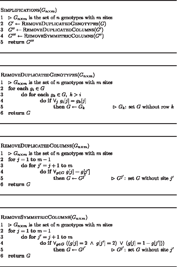
Procedure for instance simplification.

Example 3 (Simplification Techniques). Consider the set of genotypes \documentclass{aastex}\usepackage{amsbsy}\usepackage{amsfonts}\usepackage{amssymb}\usepackage{bm}\usepackage{mathrsfs}\usepackage{pifont}\usepackage{stmaryrd}\usepackage{textcomp}\usepackage{portland,xspace}\usepackage{amsmath,amsxtra}\pagestyle{empty}\DeclareMathSizes{10}{9}{7}{6} \begin{document} $${\cal G} = \{10111 , 10121 , 21022 ,10111 , 12211 \} $$\end{document} . By removing duplicated genotypes, the fourth genotype is removed and the set becomes \documentclass{aastex}\usepackage{amsbsy}\usepackage{amsfonts}\usepackage{amssymb}\usepackage{bm}\usepackage{mathrsfs}\usepackage{pifont}\usepackage{stmaryrd}\usepackage{textcomp}\usepackage{portland,xspace}\usepackage{amsmath,amsxtra}\pagestyle{empty}\DeclareMathSizes{10}{9}{7}{6} \begin{document} $${\cal G}^ \prime = \{10111 , 10121 , 21022 , 12211 \} $$\end{document} . This set is further reduced by removing duplicated sites, which implies removing the fifth site for being equal to the first site, thus becoming \documentclass{aastex}\usepackage{amsbsy}\usepackage{amsfonts}\usepackage{amssymb}\usepackage{bm}\usepackage{mathrsfs}\usepackage{pifont}\usepackage{stmaryrd}\usepackage{textcomp}\usepackage{portland,xspace}\usepackage{amsmath,amsxtra}\pagestyle{empty}\DeclareMathSizes{10}{9}{7}{6} \begin{document} $${\cal G}^{\prime \prime} = \{1011 , 1012 , 2102 , 1221 \} $$\end{document} . Finally, we may remove the third site for being symmetric to the second site, thus getting the simplified set \documentclass{aastex}\usepackage{amsbsy}\usepackage{amsfonts}\usepackage{amssymb}\usepackage{bm}\usepackage{mathrsfs}\usepackage{pifont}\usepackage{stmaryrd}\usepackage{textcomp}\usepackage{portland,xspace}\usepackage{amsmath,amsxtra}\pagestyle{empty}\DeclareMathSizes{10}{9}{7}{6} \begin{document} $${\cal G}^{\prime \prime \prime} = \{101 , 102 , 212 , 121 \} $$\end{document} .

4.2. Computing lower bounds

The method for computing the lower bound integrates three different techniques. The procedure is described in Figure 3, and consists of the composition of the routines: CliqueLowerBound, ImprovedLowerBound, and FurtherImprovedLowerBound, which are described on the following paragraphs.

OPEN IN VIEWER

FIG. 3.

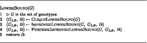
Top-level algorithm for computing lower bounds.

The techniques for computing lower bounds rely on information regarding incompatible genotypes: two genotypes are incompatible if they are both homozygous at the same site but with different values.

A lower bound can be computed from a maximal clique (Lynce and Marques-Silva, 2006). Clearly, for two incompatible genotypes, g_i and g_l, the haplotypes that explain g_i must be distinct from the haplotypes that explain g_l. Given the incompatibility relation we can create an incompatibility graph I, where each vertex is a genotype, and two vertexes are connected with an edge if they are incompatible. Suppose I has a clique of size k. Then the number of required haplotypes is at least 2k − σ, where σ is the number of genotypes in the clique which do not have heterozygous sites.

Since this problem is NP-hard (Garey and Johnson, 1979), we use the size of a clique in the incompatibility graph, computed using a simple greedy heuristic. The genotype with the highest number of incompatible genotypes is first selected. At each step, the genotype selected is one that is still incompatible with all the already selected genotypes, and preference is given to the haplotype with the highest number of incompatible genotypes. Figure 4 illustrates the algorithm which computes the clique-based lower bound.

OPEN IN VIEWER

FIG. 4.

Procedure for computing the clique-based lower bound.

Example 4 (Clique-based Lower Bounds). Consider the following set of genotypes: \documentclass{aastex}\usepackage{amsbsy}\usepackage{amsfonts}\usepackage{amssymb}\usepackage{bm}\usepackage{mathrsfs}\usepackage{pifont}\usepackage{stmaryrd}\usepackage{textcomp}\usepackage{portland,xspace}\usepackage{amsmath,amsxtra}\pagestyle{empty}\DeclareMathSizes{10}{9}{7}{6} \begin{document} $${\cal G} = \{110 , 012 , 102 \} $$\end{document} . The three genotypes are incompatible, which is represented in the incompatibility graph in Figure 5, along with each genotype contribution to the lower bound. Hence, the number of required haplotypes is at least 5 (twice the clique size less the number of genotypes with no heterozygous sites).

OPEN IN VIEWER

FIG. 5.

Clique-based lower bound.

In addition, the analysis of the structure of the genotypes allows the lower bound to be further increased, by identifying heterozygous sites which require at least one additional haplotype given a set of previously chosen genotypes (Lynce and Marques-Silva, 2008). The procedure starts from the clique-based lower bound and grows the lower bound by searching for heterozygous sites among genotypes not yet considered for lower bounding purposes. For each genotype g_i not in the clique, if the genotype has a heterozygous site and all compatible genotypes have the same value at that site (either 0 or 1), then g_i is guaranteed to require one additional haplotype to be explained. Hence the lower bound can be increased by 1. Figure 6 presents the pseudo-code of the algorithm for calculating the improved lower bound.

OPEN IN VIEWER

FIG. 6.

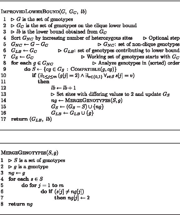
Pseudo-code for computing improved lower bounds.

Another improvement to the lower bound consists in identifying genotypes with triples of heterozygous sites, among the genotypes not used in the clique lower bound. Figure 7 presents the pseudo-code of the algorithm for calculating the lower bound based on the triples of heterozygous sites.

OPEN IN VIEWER

FIG. 7.

Pseudo-code for computing lower bounds based on triples of heterozygous sites.

Example 5 (Improved Lower Bounds). Consider the following set of genotypes: \documentclass{aastex}\usepackage{amsbsy}\usepackage{amsfonts}\usepackage{amssymb}\usepackage{bm}\usepackage{mathrsfs}\usepackage{pifont}\usepackage{stmaryrd}\usepackage{textcomp}\usepackage{portland,xspace}\usepackage{amsmath,amsxtra}\pagestyle{empty}\DeclareMathSizes{10}{9}{7}{6} \begin{document} $${\cal G} = \{200 , 020 ,002 , 222 \} $$\end{document} . Given that there are no two incompatible genotypes, the clique-based lower bound would give a lower bound of 2 corresponding to a unique vertex (e.g., with the first genotype). The analysis of the structure of the remaining genotypes requires one additional haplotype for the second and the third genotype, thus increasing the lower bound to 4 haplotypes. This lower bound can be further improved by analyzing the fourth haplotype 222. Any of the haplotypes already included in the lower bound requires at least two positions with value 0. But the pair of haplotypes explaining 222 will require one haplotype with at most one position with value 0. Hence, the lower bound can be increased by 1 to 5.

4.3. Computing upper bounds

Clark's method is a well-known algorithm to solve the haplotype inference problem (Clark, 1990). This method starts by identifying genotypes with zero or one heterozygous sites, which have only one possible explanation. Then, the method attempts to explain the remaining genotypes with at least one of the haplotypes already identified. This may eventually require the inference of new haplotypes which will be added to the set of haplotypes. The key point to note is that there are many ways to extend the set of haplotypes, since for genotypes with more than one heterozygous site there are a few possible explanations.

Clark's method may be used to compute an upper bound to the HIPP problem. However, this method is often too greedy. An alternative algorithm, called “Delayed Selection” (DS) (Marques-Silva et al., 2007), addresses the main drawback of Clark's method. The DS algorithm maintains two sets of haplotypes: the selected haplotypes, which represent haplotypes which have been chosen to be included in the target solution, and the candidate haplotypes, which represent haplotypes which can explain one or more genotypes not yet explained by a pair of selected haplotypes.

The initial set of selected haplotypes corresponds to all haplotypes which are required to explain the genotypes with no more than one heterozygous site (i.e., genotypes which are explained with either one or exactly two haplotypes). At each step, the DS algorithm chooses the candidate haplotype h_c which can explain the largest number of genotypes. The chosen haplotype h_c is then used to identify additional candidate haplotypes. Moreover, h_c is added to the set of selected haplotypes, and all genotypes which can be explained by a pair of selected haplotypes are removed from the set of unexplained genotypes. The algorithm terminates when all genotypes have been explained.

Each time the set of candidate haplotypes becomes empty, and there are still genotypes to be explained, a new candidate haplotype is generated. The new haplotype is selected greedily as the haplotype which can explain the largest number of genotypes not yet explained. Given that the proposed organization allows selecting haplotypes which will not be used in the final solution, the last step of the algorithm is to remove from the set of selected haplotypes all haplotypes which are not used for explaining any genotypes. Figure 8 presents the pseudo-code of the algorithm for calculating the upper bound.

OPEN IN VIEWER

FIG. 8.

Procedure for computing upper bound.

Example 6 (Upper Bounds). Consider the set of genotypes \documentclass{aastex}\usepackage{amsbsy}\usepackage{amsfonts}\usepackage{amssymb}\usepackage{bm}\usepackage{mathrsfs}\usepackage{pifont}\usepackage{stmaryrd}\usepackage{textcomp}\usepackage{portland,xspace}\usepackage{amsmath,amsxtra}\pagestyle{empty}\DeclareMathSizes{10}{9}{7}{6} \begin{document} $${\cal G} = \{1010 , 0002 , 2211 , 2222 \} $$\end{document} . \documentclass{aastex}\usepackage{amsbsy}\usepackage{amsfonts}\usepackage{amssymb}\usepackage{bm}\usepackage{mathrsfs}\usepackage{pifont}\usepackage{stmaryrd}\usepackage{textcomp}\usepackage{portland,xspace}\usepackage{amsmath,amsxtra}\pagestyle{empty}\DeclareMathSizes{10}{9}{7}{6} \begin{document} $${\cal G}$$\end{document} has two genotypes with no more than one heterozygous site, 1010 and 0002. Therefore, the initial set of selected haplotypes is \documentclass{aastex}\usepackage{amsbsy}\usepackage{amsfonts}\usepackage{amssymb}\usepackage{bm}\usepackage{mathrsfs}\usepackage{pifont}\usepackage{stmaryrd}\usepackage{textcomp}\usepackage{portland,xspace}\usepackage{amsmath,amsxtra}\pagestyle{empty}\DeclareMathSizes{10}{9}{7}{6} \begin{document} $${\cal H}_S = \{1010 , 0000 , 0001 \} $$\end{document} . The set of unexplained genotypes is reduced to \documentclass{aastex}\usepackage{amsbsy}\usepackage{amsfonts}\usepackage{amssymb}\usepackage{bm}\usepackage{mathrsfs}\usepackage{pifont}\usepackage{stmaryrd}\usepackage{textcomp}\usepackage{portland,xspace}\usepackage{amsmath,amsxtra}\pagestyle{empty}\DeclareMathSizes{10}{9}{7}{6} \begin{document} $${\cal G}^ \prime = \{2211 , 2222 \} $$\end{document} . Using the selected haplotypes to partially explain the genotypes, a set of candidate haplotypes is defined \documentclass{aastex}\usepackage{amsbsy}\usepackage{amsfonts}\usepackage{amssymb}\usepackage{bm}\usepackage{mathrsfs}\usepackage{pifont}\usepackage{stmaryrd}\usepackage{textcomp}\usepackage{portland,xspace}\usepackage{amsmath,amsxtra}\pagestyle{empty}\DeclareMathSizes{10}{9}{7}{6} \begin{document} $${\cal H}_C = \{0101 , 1111 , 1110 \} $$\end{document} . The candidate haplotype \documentclass{aastex}\usepackage{amsbsy}\usepackage{amsfonts}\usepackage{amssymb}\usepackage{bm}\usepackage{mathrsfs}\usepackage{pifont}\usepackage{stmaryrd}\usepackage{textcomp}\usepackage{portland,xspace}\usepackage{amsmath,amsxtra}\pagestyle{empty}\DeclareMathSizes{10}{9}{7}{6} \begin{document} $$h_c \in {\cal H}_C$$\end{document} which explains the largest number of genotypes is selected, h_c = 1111. The set of selected haplotypes becomes \documentclass{aastex}\usepackage{amsbsy}\usepackage{amsfonts}\usepackage{amssymb}\usepackage{bm}\usepackage{mathrsfs}\usepackage{pifont}\usepackage{stmaryrd}\usepackage{textcomp}\usepackage{portland,xspace}\usepackage{amsmath,amsxtra}\pagestyle{empty}\DeclareMathSizes{10}{9}{7}{6} \begin{document} $${\cal H}_S^ \prime = \{1010 , 0000 , 0001 , 1111 \} $$\end{document} and new explained genotypes are removed: \documentclass{aastex}\usepackage{amsbsy}\usepackage{amsfonts}\usepackage{amssymb}\usepackage{bm}\usepackage{mathrsfs}\usepackage{pifont}\usepackage{stmaryrd}\usepackage{textcomp}\usepackage{portland,xspace}\usepackage{amsmath,amsxtra}\pagestyle{empty}\DeclareMathSizes{10}{9}{7}{6} \begin{document} $${\cal G}^{\prime \prime} = \{2211 \} $$\end{document} . Finally, using the selected haplotype 1111, a new candidate haplotype is selected, 0011, and \documentclass{aastex}\usepackage{amsbsy}\usepackage{amsfonts}\usepackage{amssymb}\usepackage{bm}\usepackage{mathrsfs}\usepackage{pifont}\usepackage{stmaryrd}\usepackage{textcomp}\usepackage{portland,xspace}\usepackage{amsmath,amsxtra}\pagestyle{empty}\DeclareMathSizes{10}{9}{7}{6} \begin{document} $${\cal H}_S^{\prime \prime} = \{1010 , 0000 , 0001 , 1111 , 0011 \} $$\end{document} . All genotypes have been explained and, therefore, the algorithm terminates. Hence, the upper bound computed by the DS algorithm is 5.

5. Solving Hipp with Integer Linear Programming

The first approaches for the HIPP problem were based on Integer Linear Programming (ILP) models, solved with dedicated solvers (Gusfield, 2003; Halldórsson et al., 2004; Brown and Harrower, 2004, 2006). These models are briefly reviewed below.

6. Solving Hipp with a Branch-and-Bound Algorithm

HAPAR ² (Wang and Xu, 2003) is a branch-and-bound algorithm designed to solve the HIPP problem.

Inspired by the RTIP model (Gusfield, 2003), HAPAR also enumerates all possible pairs of haplotypes explaining each genotype \documentclass{aastex}\usepackage{amsbsy}\usepackage{amsfonts}\usepackage{amssymb}\usepackage{bm}\usepackage{mathrsfs}\usepackage{pifont}\usepackage{stmaryrd}\usepackage{textcomp}\usepackage{portland,xspace}\usepackage{amsmath,amsxtra}\pagestyle{empty}\DeclareMathSizes{10}{9}{7}{6} \begin{document} $$g \in {\cal G}$$\end{document} . Listing all haplotype pairs is a critical task, because the number of pairs is exponential. The method includes several improvements in order to reduce the size of the lists of haplotype pairs. One significant optimization consists of eliminating pairs of haplotypes that are guaranteed not to yield solutions better than the solutions produced by other pairs of haplotypes.

The HAPAR algorithm works as follows. The initial upper bound solution to the branch-and-bound algorithm is given by a greedy algorithm which associates each genotype with the haplotype pair with maximum coverage. The coverage of an haplotype h is the number of genotypes \documentclass{aastex}\usepackage{amsbsy}\usepackage{amsfonts}\usepackage{amssymb}\usepackage{bm}\usepackage{mathrsfs}\usepackage{pifont}\usepackage{stmaryrd}\usepackage{textcomp}\usepackage{portland,xspace}\usepackage{amsmath,amsxtra}\pagestyle{empty}\DeclareMathSizes{10}{9}{7}{6} \begin{document} $$g \in {\cal G}$$\end{document} that h can explain and the coverage of an haplotype pair is the sum of the coverage of both haplotypes in the pair. The solution of this greedy algorithm is often close to the optimal solution. This step is followed by a standard branch-and-bound search. Starting with the initial greedy solution, the algorithm searches for solutions with a lower number of distinct haplotypes, cutting off and pruning the search space where a solution smaller than the current upper bound is guaranteed not to be found in the respective branch of the search tree. The pseudo-code is described in Figure 9.

OPEN IN VIEWER

FIG. 9.

Illustration of the branch-and-bound algorithm: HAPAR.

The complexity of the algorithm is \documentclass{aastex}\usepackage{amsbsy}\usepackage{amsfonts}\usepackage{amssymb}\usepackage{bm}\usepackage{mathrsfs}\usepackage{pifont}\usepackage{stmaryrd}\usepackage{textcomp}\usepackage{portland,xspace}\usepackage{amsmath,amsxtra}\pagestyle{empty}\DeclareMathSizes{10}{9}{7}{6} \begin{document} $${\cal O} ( 2^{nm})$$\end{document} , where n is the number of genotypes in the sample and m is the number of sites of each genotype.

7. Solving Hipp with Boolean Satisfiability

An alternative to solving HIPP with ILP is to use Boolean Satisfiability (SAT). The SAT problem consists in finding an assignment to n propositional variables \documentclass{aastex}\usepackage{amsbsy}\usepackage{amsfonts}\usepackage{amssymb}\usepackage{bm}\usepackage{mathrsfs}\usepackage{pifont}\usepackage{stmaryrd}\usepackage{textcomp}\usepackage{portland,xspace}\usepackage{amsmath,amsxtra}\pagestyle{empty}\DeclareMathSizes{10}{9}{7}{6} \begin{document} $$x_1 , x_2 , \ldots , x_n$$\end{document} , which satisfies the propositional formula ϕ, or deciding that there is no such assignment. Normally, the formula is represented in Conjunctive Normal Form (CNF), which corresponds to a conjunction ( \documentclass{aastex}\usepackage{amsbsy}\usepackage{amsfonts}\usepackage{amssymb}\usepackage{bm}\usepackage{mathrsfs}\usepackage{pifont}\usepackage{stmaryrd}\usepackage{textcomp}\usepackage{portland,xspace}\usepackage{amsmath,amsxtra}\pagestyle{empty}\DeclareMathSizes{10}{9}{7}{6} \begin{document} $$\wedge$$)\end{document} of clauses. A clause is a disjunction (∨) of literals. A literal is either a variable x_i or its complement \documentclass{aastex}\usepackage{amsbsy}\usepackage{amsfonts}\usepackage{amssymb}\usepackage{bm}\usepackage{mathrsfs}\usepackage{pifont}\usepackage{stmaryrd}\usepackage{textcomp}\usepackage{portland,xspace}\usepackage{amsmath,amsxtra}\pagestyle{empty}\DeclareMathSizes{10}{9}{7}{6} \begin{document} $$\neg x_i$$\end{document} . The SAT problem was the first problem proved to be NP-complete (Cook, 1971).

Current SAT solvers are characterized by being extremely fast at solving real world problem instances, mainly due to the use of very efficient data structures and the capacity to learn new constraints whenever the search reaches a dead-end. SAT-based approaches for the HIPP problem were recently proposed with the SHIPs tool ³ (Lynce and Marques-Silva, 2006, 2008), and led to remarkable performance improvements over the existing ILP-based models.

The SAT-based HIPP solution algorithm starts from a lower bound lb on the number of haplotypes necessary to explain the set of genotypes; a trivial value for lb is 1. The algorithm searches for the smallest value r such that there exists a set \documentclass{aastex}\usepackage{amsbsy}\usepackage{amsfonts}\usepackage{amssymb}\usepackage{bm}\usepackage{mathrsfs}\usepackage{pifont}\usepackage{stmaryrd}\usepackage{textcomp}\usepackage{portland,xspace}\usepackage{amsmath,amsxtra}\pagestyle{empty}\DeclareMathSizes{10}{9}{7}{6} \begin{document} $${\cal H}$$\end{document} of haplotypes with \documentclass{aastex}\usepackage{amsbsy}\usepackage{amsfonts}\usepackage{amssymb}\usepackage{bm}\usepackage{mathrsfs}\usepackage{pifont}\usepackage{stmaryrd}\usepackage{textcomp}\usepackage{portland,xspace}\usepackage{amsmath,amsxtra}\pagestyle{empty}\DeclareMathSizes{10}{9}{7}{6} \begin{document} $$r = \mid {\cal H} \mid$$\end{document} , which explain all genotypes in \documentclass{aastex}\usepackage{amsbsy}\usepackage{amsfonts}\usepackage{amssymb}\usepackage{bm}\usepackage{mathrsfs}\usepackage{pifont}\usepackage{stmaryrd}\usepackage{textcomp}\usepackage{portland,xspace}\usepackage{amsmath,amsxtra}\pagestyle{empty}\DeclareMathSizes{10}{9}{7}{6} \begin{document} $${\cal G}$$\end{document} . Observe that the value of r is guaranteed to satisfy lb ≤ r ≤ 2 n, since a solution with 2·n haplotypes is guaranteed to exist. For each value of r considered, a CNF formula φ^r is created, and a SAT solver is invoked.

In what follows the same indexes will be used throughout: i ranges over the genotypes and j over the sites, with 1 ≤ i ≤ n and 1 ≤ j ≤ m, where n is the number of genotypes and m is the number of sites. In addition, r candidate haplotypes are considered, each with m sites, and with 1 ≤ r ≤ 2·n. An additional index k is associated with haplotypes, such that 1 ≤ k ≤ r. As a result, \documentclass{aastex}\usepackage{amsbsy}\usepackage{amsfonts}\usepackage{amssymb}\usepackage{bm}\usepackage{mathrsfs}\usepackage{pifont}\usepackage{stmaryrd}\usepackage{textcomp}\usepackage{portland,xspace}\usepackage{amsmath,amsxtra}\pagestyle{empty}\DeclareMathSizes{10}{9}{7}{6} \begin{document} $$h_{kj} \in \{ 0 , 1 \} $$\end{document} denotes the j^th site of haplotype k.

For a given value of r, the SHIPs model considers r haplotypes and seeks to associate two haplotypes (possibly corresponding to the same haplotype) with each genotype g_i, where 1 ≤ i ≤ n. The Boolean variables used by SHIPs are depicted in Figure 10. For each genotype g_i the model uses selector variables for selecting which haplotypes are used for explaining g_i. Since the genotype is to be explained by two haplotypes, the model uses two sets, a and b, of r selector variables, respectively \documentclass{aastex}\usepackage{amsbsy}\usepackage{amsfonts}\usepackage{amssymb}\usepackage{bm}\usepackage{mathrsfs}\usepackage{pifont}\usepackage{stmaryrd}\usepackage{textcomp}\usepackage{portland,xspace}\usepackage{amsmath,amsxtra}\pagestyle{empty}\DeclareMathSizes{10}{9}{7}{6} \begin{document} $$s^a_{ki}$$\end{document} and \documentclass{aastex}\usepackage{amsbsy}\usepackage{amsfonts}\usepackage{amssymb}\usepackage{bm}\usepackage{mathrsfs}\usepackage{pifont}\usepackage{stmaryrd}\usepackage{textcomp}\usepackage{portland,xspace}\usepackage{amsmath,amsxtra}\pagestyle{empty}\DeclareMathSizes{10}{9}{7}{6} \begin{document} $$s^b_{ki}$$\end{document} with \documentclass{aastex}\usepackage{amsbsy}\usepackage{amsfonts}\usepackage{amssymb}\usepackage{bm}\usepackage{mathrsfs}\usepackage{pifont}\usepackage{stmaryrd}\usepackage{textcomp}\usepackage{portland,xspace}\usepackage{amsmath,amsxtra}\pagestyle{empty}\DeclareMathSizes{10}{9}{7}{6} \begin{document} $$k = 1 , \ldots , r$$\end{document} . Hence, genotype g_i is explained by haplotypes \documentclass{aastex}\usepackage{amsbsy}\usepackage{amsfonts}\usepackage{amssymb}\usepackage{bm}\usepackage{mathrsfs}\usepackage{pifont}\usepackage{stmaryrd}\usepackage{textcomp}\usepackage{portland,xspace}\usepackage{amsmath,amsxtra}\pagestyle{empty}\DeclareMathSizes{10}{9}{7}{6} \begin{document} $$h_{k_1}$$\end{document} and \documentclass{aastex}\usepackage{amsbsy}\usepackage{amsfonts}\usepackage{amssymb}\usepackage{bm}\usepackage{mathrsfs}\usepackage{pifont}\usepackage{stmaryrd}\usepackage{textcomp}\usepackage{portland,xspace}\usepackage{amsmath,amsxtra}\pagestyle{empty}\DeclareMathSizes{10}{9}{7}{6} \begin{document} $$h_{k_2}$$\end{document} if \documentclass{aastex}\usepackage{amsbsy}\usepackage{amsfonts}\usepackage{amssymb}\usepackage{bm}\usepackage{mathrsfs}\usepackage{pifont}\usepackage{stmaryrd}\usepackage{textcomp}\usepackage{portland,xspace}\usepackage{amsmath,amsxtra}\pagestyle{empty}\DeclareMathSizes{10}{9}{7}{6} \begin{document} $$s^a_{k_1i} = 1$$\end{document} and \documentclass{aastex}\usepackage{amsbsy}\usepackage{amsfonts}\usepackage{amssymb}\usepackage{bm}\usepackage{mathrsfs}\usepackage{pifont}\usepackage{stmaryrd}\usepackage{textcomp}\usepackage{portland,xspace}\usepackage{amsmath,amsxtra}\pagestyle{empty}\DeclareMathSizes{10}{9}{7}{6} \begin{document} $$s^b_{k_2i} = 1$$\end{document} . Clearly, g_i is also explained by the same haplotypes if \documentclass{aastex}\usepackage{amsbsy}\usepackage{amsfonts}\usepackage{amssymb}\usepackage{bm}\usepackage{mathrsfs}\usepackage{pifont}\usepackage{stmaryrd}\usepackage{textcomp}\usepackage{portland,xspace}\usepackage{amsmath,amsxtra}\pagestyle{empty}\DeclareMathSizes{10}{9}{7}{6} \begin{document} $$s^a_{k_2i} = 1$$\end{document} and \documentclass{aastex}\usepackage{amsbsy}\usepackage{amsfonts}\usepackage{amssymb}\usepackage{bm}\usepackage{mathrsfs}\usepackage{pifont}\usepackage{stmaryrd}\usepackage{textcomp}\usepackage{portland,xspace}\usepackage{amsmath,amsxtra}\pagestyle{empty}\DeclareMathSizes{10}{9}{7}{6} \begin{document} $$s^b_{k_1 \ i} = 1$$\end{document} .

OPEN IN VIEWER

FIG. 10.

Boolean variables used in SHIPs.

We can now derive the conditions for the SHIPs model:

If a site g_ij is 0 (resp. 1), and if haplotype k is selected for explaining genotype i, either by the a or the b representative, then the value of haplotype k at site j must be 0 (resp. 1). In CNF, if site g_ij is 0, then the model includes \documentclass{aastex}\usepackage{amsbsy}\usepackage{amsfonts}\usepackage{amssymb}\usepackage{bm}\usepackage{mathrsfs}\usepackage{pifont}\usepackage{stmaryrd}\usepackage{textcomp}\usepackage{portland,xspace}\usepackage{amsmath,amsxtra}\pagestyle{empty}\DeclareMathSizes{10}{9}{7}{6} \begin{document} $$( \neg s^a_{ki} \vee \neg h_{k \, j}) \wedge ( \neg s^b_{ki} \vee \neg h_{k \, j})$$\end{document} , and if site g_ij is 1, then the model includes \documentclass{aastex}\usepackage{amsbsy}\usepackage{amsfonts}\usepackage{amssymb}\usepackage{bm}\usepackage{mathrsfs}\usepackage{pifont}\usepackage{stmaryrd}\usepackage{textcomp}\usepackage{portland,xspace}\usepackage{amsmath,amsxtra}\pagestyle{empty}\DeclareMathSizes{10}{9}{7}{6} \begin{document} $$( \neg s^a_{ki} \vee h_{kj}) \wedge ( \neg s^b_{ki} \vee h_{k \,j})$$\end{document} , in both cases for \documentclass{aastex}\usepackage{amsbsy}\usepackage{amsfonts}\usepackage{amssymb}\usepackage{bm}\usepackage{mathrsfs}\usepackage{pifont}\usepackage{stmaryrd}\usepackage{textcomp}\usepackage{portland,xspace}\usepackage{amsmath,amsxtra}\pagestyle{empty}\DeclareMathSizes{10}{9}{7}{6} \begin{document} $$k = 1 , \ldots , r$$\end{document} .

Clearly, for each genotype g_i, and for a or b, it is necessary that exactly one haplotype is used, and so exactly one selector variable can be assigned value 1. This can be captured with the following cardinality constraints: \documentclass{aastex}\usepackage{amsbsy}\usepackage{amsfonts}\usepackage{amssymb}\usepackage{bm}\usepackage{mathrsfs}\usepackage{pifont}\usepackage{stmaryrd}\usepackage{textcomp}\usepackage{portland,xspace}\usepackage{amsmath,amsxtra}\pagestyle{empty}\DeclareMathSizes{10}{9}{7}{6} \begin{document} \begin{align*} \left( \sum_{k = 1}^r s^a_{k \, i} = 1 \right) \wedge \left( \sum_{k = 1}^r s^b_{k \, i} = 1 \right). \tag{6}\end{align*} \end{document}

These cardinality constraints can be encoded in CNF in linear space, by introducing additional auxiliary variables (Lynce and Marques-Silva, 2006, 2008).

Besides the basic model outlined above, SAT-based haplotyping requires the inclusion of a number of effective techniques, including lower bounds (see Section 4.2) and identification of symmetries (Lynce and Marques-Silva, 2006). More recent work addressed using local search algorithms for improving lower bounds in SAT-based approaches for the HIPP problem (Lynce et al., 2008b).

8. Solving Hipp with Pseudo-Boolean Optimization

The success of solving HIPP with SAT motivated considering other Boolean-based decision and optimization procedures. One very successful approach is based on using Pseudo-Boolean Optimization (PBO) in a tool called RPoly ⁵ (Graça et al., 2007, 2008). A PBO problem, also known as 0-1 integer linear programming (0-1 ILP), is an ILP problem which uses only Boolean variables.

The organization of RPoly is similar to the organization of PolyIP: two haplotypes are associated with each genotype, and conditions which capture when a different haplotype is used for explaining a given genotype are defined. With no surprise, the generated PBO formulas are much larger than the generated SAT formulas for a given HIPP problem instance. Whereas the PBO approach assumes the worst case for which the number of required haplotypes is twice the number of genotypes, the SAT approach incrementally increases the number of required haplotypes starting from a lower bound.

Despite the similarities, RPoly has a few key differences with respect to PolyIP (Brown and Harrower, 2004). First, the set of variables is different. Instead of associating a variable with each site of each haplotype, RPoly only associates variables with heterozygous sites (since the value of haplotypes in the other sites is known beforehand, and so can be implicitly assumed). In addition, each used variable describes the possible pairs of values for the corresponding heterozygous site.

In practice, the model associates two haplotypes, \documentclass{aastex}\usepackage{amsbsy}\usepackage{amsfonts}\usepackage{amssymb}\usepackage{bm}\usepackage{mathrsfs}\usepackage{pifont}\usepackage{stmaryrd}\usepackage{textcomp}\usepackage{portland,xspace}\usepackage{amsmath,amsxtra}\pagestyle{empty}\DeclareMathSizes{10}{9}{7}{6} \begin{document} $$h^a_i$$\end{document} and \documentclass{aastex}\usepackage{amsbsy}\usepackage{amsfonts}\usepackage{amssymb}\usepackage{bm}\usepackage{mathrsfs}\usepackage{pifont}\usepackage{stmaryrd}\usepackage{textcomp}\usepackage{portland,xspace}\usepackage{amsmath,amsxtra}\pagestyle{empty}\DeclareMathSizes{10}{9}{7}{6} \begin{document} $$h^b_i$$\end{document} , with each genotype g_i, and these haplotypes are required to explain g_i. Moreover, the model associates a variable t_ij with each heterozygous site (i, j) (i.e., with g_ij = 2). Hence, t_ij = 1 indicates that \documentclass{aastex}\usepackage{amsbsy}\usepackage{amsfonts}\usepackage{amssymb}\usepackage{bm}\usepackage{mathrsfs}\usepackage{pifont}\usepackage{stmaryrd}\usepackage{textcomp}\usepackage{portland,xspace}\usepackage{amsmath,amsxtra}\pagestyle{empty}\DeclareMathSizes{10}{9}{7}{6} \begin{document} $$h^a_{i \, j} = 1$$\end{document} and \documentclass{aastex}\usepackage{amsbsy}\usepackage{amsfonts}\usepackage{amssymb}\usepackage{bm}\usepackage{mathrsfs}\usepackage{pifont}\usepackage{stmaryrd}\usepackage{textcomp}\usepackage{portland,xspace}\usepackage{amsmath,amsxtra}\pagestyle{empty}\DeclareMathSizes{10}{9}{7}{6} \begin{document} $$h^b_{i \, j} = 0$$\end{document} , whereas t_ij = 0 indicates that \documentclass{aastex}\usepackage{amsbsy}\usepackage{amsfonts}\usepackage{amssymb}\usepackage{bm}\usepackage{mathrsfs}\usepackage{pifont}\usepackage{stmaryrd}\usepackage{textcomp}\usepackage{portland,xspace}\usepackage{amsmath,amsxtra}\pagestyle{empty}\DeclareMathSizes{10}{9}{7}{6} \begin{document} $$h^a_{i \,j} = 0$$\end{document} and \documentclass{aastex}\usepackage{amsbsy}\usepackage{amsfonts}\usepackage{amssymb}\usepackage{bm}\usepackage{mathrsfs}\usepackage{pifont}\usepackage{stmaryrd}\usepackage{textcomp}\usepackage{portland,xspace}\usepackage{amsmath,amsxtra}\pagestyle{empty}\DeclareMathSizes{10}{9}{7}{6} \begin{document} $$h^b_{i \, j} = 1$$\end{document} . The value of \documentclass{aastex}\usepackage{amsbsy}\usepackage{amsfonts}\usepackage{amssymb}\usepackage{bm}\usepackage{mathrsfs}\usepackage{pifont}\usepackage{stmaryrd}\usepackage{textcomp}\usepackage{portland,xspace}\usepackage{amsmath,amsxtra}\pagestyle{empty}\DeclareMathSizes{10}{9}{7}{6} \begin{document} $$h^a_i$$\end{document} and \documentclass{aastex}\usepackage{amsbsy}\usepackage{amsfonts}\usepackage{amssymb}\usepackage{bm}\usepackage{mathrsfs}\usepackage{pifont}\usepackage{stmaryrd}\usepackage{textcomp}\usepackage{portland,xspace}\usepackage{amsmath,amsxtra}\pagestyle{empty}\DeclareMathSizes{10}{9}{7}{6} \begin{document} $$h^b_i$$\end{document} at homozygous sites j is implicitly assumed. The symmetry in a pair of haplotypes is broken by considering that t_ij = 0 for the first heterozygous site g_ij of each genotype g_i.

This alternative definition of the variables associated with the sites of genotypes reduces the number of variables by a factor of 2: instead of associating two variables with each site, RPoly associates a single variable with each site. In addition, the model only creates variables for heterozygous sites, and, therefore, the number of variables associated with sites equals the total number of heterozygous sites. As a result, the conditions provided by equations (2) of the PolyIP model are eliminated. It is interesting to observe that this definition of the variables associated with sites follows the SHIPs model (Lynce and Marques-Silva, 2006, 2008).

Finally, another key modification is that the candidate haplotypes for each genotype are related with candidate haplotypes for other genotypes only if the two genotypes are compatible. Clearly, incompatible genotypes are guaranteed not to be explained by the same haplotype.

The proposed modification implies the use of two additional sets of variables. Variable \documentclass{aastex}\usepackage{amsbsy}\usepackage{amsfonts}\usepackage{amssymb}\usepackage{bm}\usepackage{mathrsfs}\usepackage{pifont}\usepackage{stmaryrd}\usepackage{textcomp}\usepackage{portland,xspace}\usepackage{amsmath,amsxtra}\pagestyle{empty}\DeclareMathSizes{10}{9}{7}{6} \begin{document} $$x^{p \ q}_{i_1 \ i_2}$$\end{document} , with \documentclass{aastex}\usepackage{amsbsy}\usepackage{amsfonts}\usepackage{amssymb}\usepackage{bm}\usepackage{mathrsfs}\usepackage{pifont}\usepackage{stmaryrd}\usepackage{textcomp}\usepackage{portland,xspace}\usepackage{amsmath,amsxtra}\pagestyle{empty}\DeclareMathSizes{10}{9}{7}{6} \begin{document} $$p , q \in \{a , b \} $$\end{document} and 1 ≤ i₂ < i₁ ≤ n, is 1 if the p haplotype of genotype g_i1 and the q haplotype of genotype g_i2 are different. If genotypes g _{i 1} and g _{i 2} are incompatible, then the value of \documentclass{aastex}\usepackage{amsbsy}\usepackage{amsfonts}\usepackage{amssymb}\usepackage{bm}\usepackage{mathrsfs}\usepackage{pifont}\usepackage{stmaryrd}\usepackage{textcomp}\usepackage{portland,xspace}\usepackage{amsmath,amsxtra}\pagestyle{empty}\DeclareMathSizes{10}{9}{7}{6} \begin{document} $$x^{p \ q}_{i_1 \ i_2}$$\end{document} is 1 for the four possible combinations of p and q. Moreover, two genotypes g _{i 1} and g _{i 2} are related only with respect to sites j such that either g _{i 1} or g _{i 2} is heterozygous at that site. In addition, the model uses variables to denote when one of the haplotypes associated with a given genotype is different from all previous haplotypes. Hence, \documentclass{aastex}\usepackage{amsbsy}\usepackage{amsfonts}\usepackage{amssymb}\usepackage{bm}\usepackage{mathrsfs}\usepackage{pifont}\usepackage{stmaryrd}\usepackage{textcomp}\usepackage{portland,xspace}\usepackage{amsmath,amsxtra}\pagestyle{empty}\DeclareMathSizes{10}{9}{7}{6} \begin{document} $$u^p_i$$\end{document} , with \documentclass{aastex}\usepackage{amsbsy}\usepackage{amsfonts}\usepackage{amssymb}\usepackage{bm}\usepackage{mathrsfs}\usepackage{pifont}\usepackage{stmaryrd}\usepackage{textcomp}\usepackage{portland,xspace}\usepackage{amsmath,amsxtra}\pagestyle{empty}\DeclareMathSizes{10}{9}{7}{6} \begin{document} $$p \in \{a , b \} $$\end{document} and 1 ≤ i ≤ n, is 1 if haplotype p of genotype g_i is different from all previous haplotypes.

The conditions on the \documentclass{aastex}\usepackage{amsbsy}\usepackage{amsfonts}\usepackage{amssymb}\usepackage{bm}\usepackage{mathrsfs}\usepackage{pifont}\usepackage{stmaryrd}\usepackage{textcomp}\usepackage{portland,xspace}\usepackage{amsmath,amsxtra}\pagestyle{empty}\DeclareMathSizes{10}{9}{7}{6} \begin{document} $$u^p_i$$\end{document} variables are based on the conditions for the x_i variables for the PolyIP model, \documentclass{aastex}\usepackage{amsbsy}\usepackage{amsfonts}\usepackage{amssymb}\usepackage{bm}\usepackage{mathrsfs}\usepackage{pifont}\usepackage{stmaryrd}\usepackage{textcomp}\usepackage{portland,xspace}\usepackage{amsmath,amsxtra}\pagestyle{empty}\DeclareMathSizes{10}{9}{7}{6} \begin{document} \begin{align*} \bigwedge_{1 \leq k < i} ( x^{p \ a}_{i \ k} \wedge x^{p \ b}_{i \ k}) \rightarrow u^{p}_{i}. \tag{7}\end{align*} \end{document}

The conditions on the \documentclass{aastex}\usepackage{amsbsy}\usepackage{amsfonts}\usepackage{amssymb}\usepackage{bm}\usepackage{mathrsfs}\usepackage{pifont}\usepackage{stmaryrd}\usepackage{textcomp}\usepackage{portland,xspace}\usepackage{amsmath,amsxtra}\pagestyle{empty}\DeclareMathSizes{10}{9}{7}{6} \begin{document} $$x^{p \ q}_{i_1 \ i_2}$$\end{document} variables are all of the following form, for all 1 ≤ j ≤ m: \documentclass{aastex}\usepackage{amsbsy}\usepackage{amsfonts}\usepackage{amssymb}\usepackage{bm}\usepackage{mathrsfs}\usepackage{pifont}\usepackage{stmaryrd}\usepackage{textcomp}\usepackage{portland,xspace}\usepackage{amsmath,amsxtra}\pagestyle{empty}\DeclareMathSizes{10}{9}{7}{6} \begin{document} \begin{align*} \neg ( R \leftrightarrow S ) \rightarrow x^{p \ q}_{i_1 \ i_2} , \tag{8}\end{align*} \end{document}

where the predicates R and S depend on the values of the sites (i₁, j) and (i₂, j), and on which of the haplotypes is considered, i.e. either a or b. Observe that 1 ≤ i₂ < i₁ ≤ n, 1 ≤ j ≤ m, and \documentclass{aastex}\usepackage{amsbsy}\usepackage{amsfonts}\usepackage{amssymb}\usepackage{bm}\usepackage{mathrsfs}\usepackage{pifont}\usepackage{stmaryrd}\usepackage{textcomp}\usepackage{portland,xspace}\usepackage{amsmath,amsxtra}\pagestyle{empty}\DeclareMathSizes{10}{9}{7}{6} \begin{document} $$p , q \in \{a , b \} $$\end{document} . Accordingly, the R and S predicates are defined as follows:

If \documentclass{aastex}\usepackage{amsbsy}\usepackage{amsfonts}\usepackage{amssymb}\usepackage{bm}\usepackage{mathrsfs}\usepackage{pifont}\usepackage{stmaryrd}\usepackage{textcomp}\usepackage{portland,xspace}\usepackage{amsmath,amsxtra}\pagestyle{empty}\DeclareMathSizes{10}{9}{7}{6} \begin{document} $$g_{i_1j} \neq 2$$\end{document} , then \documentclass{aastex}\usepackage{amsbsy}\usepackage{amsfonts}\usepackage{amssymb}\usepackage{bm}\usepackage{mathrsfs}\usepackage{pifont}\usepackage{stmaryrd}\usepackage{textcomp}\usepackage{portland,xspace}\usepackage{amsmath,amsxtra}\pagestyle{empty}\DeclareMathSizes{10}{9}{7}{6} \begin{document} $$g_{i_1j} \leftrightarrow ( q \leftrightarrow a ) )$$\end{document} and \documentclass{aastex}\usepackage{amsbsy}\usepackage{amsfonts}\usepackage{amssymb}\usepackage{bm}\usepackage{mathrsfs}\usepackage{pifont}\usepackage{stmaryrd}\usepackage{textcomp}\usepackage{portland,xspace}\usepackage{amsmath,amsxtra}\pagestyle{empty}\DeclareMathSizes{10}{9}{7}{6} \begin{document} $$S = t_{i_2j}$$\end{document} .

Finally, the cost function is given by: \documentclass{aastex}\usepackage{amsbsy}\usepackage{amsfonts}\usepackage{amssymb}\usepackage{bm}\usepackage{mathrsfs}\usepackage{pifont}\usepackage{stmaryrd}\usepackage{textcomp}\usepackage{portland,xspace}\usepackage{amsmath,amsxtra}\pagestyle{empty}\DeclareMathSizes{10}{9}{7}{6} \begin{document} \begin{align*} {\rm minimize} \sum^{n}_{i = 1} ( u^{a}_{i} + u^{b}_{i}). \tag{9}\end{align*} \end{document}

The proposed simplifications to the PolyIP model (Brown and Harrower, 2004) yield significant performance improvements, even when the two models are solved with a PBO solver (Graça et al., 2007). More recently, a number of improvements to RPoly were proposed (Graça et al., 2008). Similarly to SHIPs, one of the proposed improvements is the integration of lower bounds (see Section 4.2). The lower bound procedure provides a list of genotypes with an indication of the contribution of each genotype to the lower bound. Each genotype either contributes with +2, indicating that 2 new haplotypes will be required for explaining this genotype, or with +1, indicating that 1 new haplotype will be required for explaining this genotype. For each genotype with an associated fixed haplotype, the corresponding u variable is assigned value 1, and the clauses used for constraining the value of u need not be generated. Similarly to the advantages of using lower bounds in SHIPs (Lynce et al., 2008b), the integration of lower bounds in RPoly offers a few relevant advantages. First, several u variables become fixed with value 1. This allows the PBO solver to focus on the remaining u variables. Second, the size of the generated PBO problem instances becomes significantly smaller. For the more complex problem instances, the integration of lower bound information reduces the size of the generated PBO instances by a factor between 2 and 3, on average.

Most often real genotype data contains a significant percentage of unknown data. Even with modern automated DNA analysis techniques, generating data with missing alleles is not an uncommon situation (Kelly et al., 2004). One useful feature of the RPoly tool is to be able to deal with unspecified genotype sites. Most of the HIPP solvers described above do not consider missing genotype sites, with exception of SATlotyper. Genotyping tools often leave a percentage of missing genotype positions, and so haplotype inference tools need to be able to deal with missing sites. RPoly can handle SNPs with unspecified values, inferring the values for the missing sites and still guaranteeing a parsimonious solution. Two Boolean variables are associated with each missing site to represent the four possible values for the haplotypes: two homozygous values (one for each allele) and two heterozygous values (one for each haplotype phase). The constraints for unspecified genotype sites are similar to the constraints for heterozygous genotype sites.

9. Solving Hipp with Answer Set Programming

A recent contribution to the HIPP problem uses Answer Set Programming (ASP) in a tool called HAPLO-ASP ⁶ (Erdem and Türe, 2008). ASP is a declarative programming paradigm that provides a high-level language to represent combinatorial search problems, and efficient solvers to compute solutions for them. ASP aims to represent a computational problem as a program whose models (called answer sets) correspond to the solution of the problem (Niemelä, 1999). Syntactically, ASP programs look like Prolog programs. The data types in ASP are terms which can be atoms, variables, numbers or compound terms (which are composed of atoms applied to arguments). The programs are described with rules of the form \documentclass{aastex}\usepackage{amsbsy}\usepackage{amsfonts}\usepackage{amssymb}\usepackage{bm}\usepackage{mathrsfs}\usepackage{pifont}\usepackage{stmaryrd}\usepackage{textcomp}\usepackage{portland,xspace}\usepackage{amsmath,amsxtra}\pagestyle{empty}\DeclareMathSizes{10}{9}{7}{6} \begin{document} \begin{align*} {\rm H} : \hbox{- } \ {\rm B}1 , \ldots , {\rm Bn}.\end{align*} \end{document}

which represents that H is true if \documentclass{aastex}\usepackage{amsbsy}\usepackage{amsfonts}\usepackage{amssymb}\usepackage{bm}\usepackage{mathrsfs}\usepackage{pifont}\usepackage{stmaryrd}\usepackage{textcomp}\usepackage{portland,xspace}\usepackage{amsmath,amsxtra}\pagestyle{empty}\DeclareMathSizes{10}{9}{7}{6} \begin{document} $${B1 , \ldots , Bn}$$\end{document} are true.

Rules of the form \documentclass{aastex}\usepackage{amsbsy}\usepackage{amsfonts}\usepackage{amssymb}\usepackage{bm}\usepackage{mathrsfs}\usepackage{pifont}\usepackage{stmaryrd}\usepackage{textcomp}\usepackage{portland,xspace}\usepackage{amsmath,amsxtra}\pagestyle{empty}\DeclareMathSizes{10}{9}{7}{6} \begin{document} \begin{align*} {\rm H}.\end{align*} \end{document}

are equivalent to \documentclass{aastex}\usepackage{amsbsy}\usepackage{amsfonts}\usepackage{amssymb}\usepackage{bm}\usepackage{mathrsfs}\usepackage{pifont}\usepackage{stmaryrd}\usepackage{textcomp}\usepackage{portland,xspace}\usepackage{amsmath,amsxtra}\pagestyle{empty}\DeclareMathSizes{10}{9}{7}{6} \begin{document} \begin{align*} {\rm H} : \hbox{- } \ true.\end{align*} \end{document}

which means that H must be true. In addition, rules of the form \documentclass{aastex}\usepackage{amsbsy}\usepackage{amsfonts}\usepackage{amssymb}\usepackage{bm}\usepackage{mathrsfs}\usepackage{pifont}\usepackage{stmaryrd}\usepackage{textcomp}\usepackage{portland,xspace}\usepackage{amsmath,amsxtra}\pagestyle{empty}\DeclareMathSizes{10}{9}{7}{6} \begin{document} \begin{align*} : \hbox{- } \ {\rm B}1 , \ldots , {\rm B}n.\end{align*} \end{document}

are equivalent to \documentclass{aastex}\usepackage{amsbsy}\usepackage{amsfonts}\usepackage{amssymb}\usepackage{bm}\usepackage{mathrsfs}\usepackage{pifont}\usepackage{stmaryrd}\usepackage{textcomp}\usepackage{portland,xspace}\usepackage{amsmath,amsxtra}\pagestyle{empty}\DeclareMathSizes{10}{9}{7}{6} \begin{document} \begin{align*} false : \hbox{- } \ {\rm B} 1 , \ldots , {\rm Bn}.\end{align*} \end{document}

which means that one of the terms Bi, 1 ≤ i ≤ n, must be false.

The HAPLO-ASP solver, similarly to SHIPs, is an iterative algorithm. A binary search is performed in order to find the optimal value between the lower bound (lb) and the upper bound (ub). At each iteration, an ASP formulation is solved, which decides whether there exists a solution to the haplotype inference using k distinct haplotypes, lb ≤ k ≤ ub. Clearly, if there is a haplotype inference solution using k distinct haplotypes and there exists no solution using k-1 haplotypes, then k corresponds to the number of haplotypes on the HIPP solution.

The ASP formulation is explained in the input language of the answer set solver CMODELS (Giunchiglia et al., 2006) and the grounder LPARSE (Simons et al., 2002). For a fixed number k of candidate haplotypes, the ASP formulation is as follows, with genotypes and haplotypes being considered as sets of atoms. Considering n genotypes each with m sites, and the corresponding 2n haplotypes, the rules are \documentclass{aastex}\usepackage{amsbsy}\usepackage{amsfonts}\usepackage{amssymb}\usepackage{bm}\usepackage{mathrsfs}\usepackage{pifont}\usepackage{stmaryrd}\usepackage{textcomp}\usepackage{portland,xspace}\usepackage{amsmath,amsxtra}\pagestyle{empty}\DeclareMathSizes{10}{9}{7}{6} \begin{document} \begin{align*} & geno ( 1 \ldots {\rm n}). \\ & site ( 1 \ldots {\rm m}). \\ & haplo ( 1 \ldots 2*{\rm n}).\end{align*} \end{document}

In the answer set, atom amb(i, j) represents g_ij = 2 (heterozygous site), atom -amb(i, j) represents g_ij = 1, and the absence of both positive and negative atoms represents g_ij = 0. Moreover, each genotype g_i is associated with two haplotypes, h_2i − 1 and h_2i, and each haplotype h_i is described by atoms with the form h(i, j), with 1 ≤ i ≤ 2n and 1 ≤ j ≤ m. If h(i, j) is in the answer set then h_i[j] = 1, otherwise h_i[j] = 0. Then, to generate a value for site J of haplotype H, the rules are \documentclass{aastex}\usepackage{amsbsy}\usepackage{amsfonts}\usepackage{amssymb}\usepackage{bm}\usepackage{mathrsfs}\usepackage{pifont}\usepackage{stmaryrd}\usepackage{textcomp}\usepackage{portland,xspace}\usepackage{amsmath,amsxtra}\pagestyle{empty}\DeclareMathSizes{10}{9}{7}{6} \begin{document} \begin{align*} \{h ( {\rm H} , {\rm J}) \} : \hbox{- } \ haplo ( {\rm H}) , \ site ( {\rm J}).\end{align*} \end{document}

Rules must enforce that for every heterozygous site J on genotype G, the values of haplotypes 2*G and 2*G-1 at site J cannot be both 1 or 0: \documentclass{aastex}\usepackage{amsbsy}\usepackage{amsfonts}\usepackage{amssymb}\usepackage{bm}\usepackage{mathrsfs}\usepackage{pifont}\usepackage{stmaryrd}\usepackage{textcomp}\usepackage{portland,xspace}\usepackage{amsmath,amsxtra}\pagestyle{empty}\DeclareMathSizes{10}{9}{7}{6} \begin{document} \begin{align*} & : \hbox{-} \ amb ({\rm G} , {\rm J}) , \ h (2^{*}{\rm G} , {\rm J}) , \ {\rm h} ( 2^*{\rm G} \ \hbox{-} \ 1 , {\rm J}) , \ geno ({\rm G}) , \ site ({\rm J}). \\ & : \hbox{-} \ amb ({\rm G} , {\rm J}) , \ {\rm not} \ h (2^*{\rm G} \ \hbox{-} \ 1 , {\rm J}) , \ {\rm not} \ {\rm h} (2^{*}{\rm G} , {\rm J}) , geno ({\rm G}) , \ site ({\rm J}).\end{align*} \end{document}

For every homozygous site J with value 1 in genotype G, the values of haplotypes 2*G and 2*G-1 at site J must be both 1, which is represented with rules: \documentclass{aastex}\usepackage{amsbsy}\usepackage{amsfonts}\usepackage{amssymb}\usepackage{bm}\usepackage{mathrsfs}\usepackage{pifont}\usepackage{stmaryrd}\usepackage{textcomp}\usepackage{portland,xspace}\usepackage{amsmath,amsxtra}\pagestyle{empty}\DeclareMathSizes{10}{9}{7}{6} \begin{document} \begin{align*} & : \hbox{- } \ {\rm not} \ h ( 2^{*}{\rm G} \hbox{ - }1 , {\rm J}) , \ \hbox{- }amb ( {\rm G} , {\rm J}) , \ geno ( {\rm G}) , \ site ( {\rm J}). \\ & : \hbox{- } \ {\rm not} \ h ( 2^{*}{\rm G} , {\rm J}) , \ \hbox{- }amb ( {\rm G} , {\rm J}) , geno ( {\rm G}) , \ site ( {\rm J}).\end{align*} \end{document}

Similarly, for every homozygous site J with value 0 in genotype G, the values of haplotypes 2*G and 2*G − 1 at site J must be both 0, which is represented with rules: \documentclass{aastex}\usepackage{amsbsy}\usepackage{amsfonts}\usepackage{amssymb}\usepackage{bm}\usepackage{mathrsfs}\usepackage{pifont}\usepackage{stmaryrd}\usepackage{textcomp}\usepackage{portland,xspace}\usepackage{amsmath,amsxtra}\pagestyle{empty}\DeclareMathSizes{10}{9}{7}{6} \begin{document} \begin{align*} & : \hbox{- } \ h ( 2^{*}{\rm G} \hbox{ - }1 , {\rm J}) , {\rm not} \ \hbox{- } amb ( {\rm G} , {\rm J}) , \ {\rm not} \ amb ( {\rm G} , {\rm J}) , \ geno ( {\rm G}) , \ site ( {\rm J}). \\ & : \hbox{- } \ h ( 2^{*}{\rm G} , {\rm J}) , \ {\rm not} \ \hbox{- } amb ( {\rm G} , {\rm J}) , {\rm not} \ amb ( {\rm G} , {\rm J}) , geno ( {\rm G}) , \ site ( {\rm J}).\end{align*} \end{document}

The following rules guarantee that the number of distinct haplotypes used is exactly k: \documentclass{aastex}\usepackage{amsbsy}\usepackage{amsfonts}\usepackage{amssymb}\usepackage{bm}\usepackage{mathrsfs}\usepackage{pifont}\usepackage{stmaryrd}\usepackage{textcomp}\usepackage{portland,xspace}\usepackage{amsmath,amsxtra}\pagestyle{empty}\DeclareMathSizes{10}{9}{7}{6} \begin{document} \begin{align*} diffsite ( {\rm H}1 , {\rm H} 2 , {\rm J}) : \hbox{- } \ 1 \{h ( {\rm H}1 , {\rm J}) , \ h ( {\rm H}2 , {\rm J}) \} 1 , \ haplo ( {\rm H}1{\rm ;}{\, \rm H}2 ) , \ H1 < H2 , \ site ( {\rm J}).\end{align*} \end{document}

where 1{h(H1,J), h(H2,J)}1 means that exactly one of the terms h(H1, J) and h(H2, J) is true, and therefore diffsite(H1, H2, J) is true if H1 < H2 and H1[J] ≠ H2[J], i.e., \documentclass{aastex}\usepackage{amsbsy}\usepackage{amsfonts}\usepackage{amssymb}\usepackage{bm}\usepackage{mathrsfs}\usepackage{pifont}\usepackage{stmaryrd}\usepackage{textcomp}\usepackage{portland,xspace}\usepackage{amsmath,amsxtra}\pagestyle{empty}\DeclareMathSizes{10}{9}{7}{6} \begin{document} \begin{align*} diffhapp ( {\rm H}1 , {\rm H}2 ) : \hbox{- } \ 1 \{diffsite ( {\rm H}1 , {\rm H}2 , {\rm J}) : \ site ( {\rm J}) \} , \ haplo ( {\rm H}1;{\rm H}2 ) , \ H1 < H2.\end{align*} \end{document}

where 1{diffsite(H1,H2,J) : site(J)} means that at least one of the terms diffsite(H1,H2,J), for 1 ≤ J ≤ m, is true, and diffhapp(H1, H2) is true if haplotype H1 is different from haplotype H2. The atom unique(H) describes that haplotype H is different from all haplotypes H1 with H1 < H, i.e., \documentclass{aastex}\usepackage{amsbsy}\usepackage{amsfonts}\usepackage{amssymb}\usepackage{bm}\usepackage{mathrsfs}\usepackage{pifont}\usepackage{stmaryrd}\usepackage{textcomp}\usepackage{portland,xspace}\usepackage{amsmath,amsxtra}\pagestyle{empty}\DeclareMathSizes{10}{9}{7}{6} \begin{document} \begin{align*} unique ( {\rm H}) : \hbox{- } \ {\rm H} \hbox{ - }1 \{diffhapp ( {\rm H}1 , {\rm H}) : \ haplo ( {\rm H}1 ) \} , \ haplo ( {\rm H}).\end{align*} \end{document}

where H-1{diffhapp(H1,H): haplo(H1)} represents that at least H-1 of the haplotypes H1, 1 ≤ H1 < H, are distinct of H.

Finally, the rule \documentclass{aastex}\usepackage{amsbsy}\usepackage{amsfonts}\usepackage{amssymb}\usepackage{bm}\usepackage{mathrsfs}\usepackage{pifont}\usepackage{stmaryrd}\usepackage{textcomp}\usepackage{portland,xspace}\usepackage{amsmath,amsxtra}\pagestyle{empty}\DeclareMathSizes{10}{9}{7}{6} \begin{document} \begin{align*} : \hbox{- } \ k + 1 \{unique ( {\rm H}) : \ haplo ( {\rm H}) \} .\end{align*} \end{document}

expresses that the number of unique haplotypes included in an answer set cannot be more than k.

10. Complexity of Hipp

The HIPP problem is NP-hard (Hubbell, 2000) and, furthermore, proved to be APX-hard (Lancia et al., 2004). Therefore, there is a constant λ > 1 for which there does not exist a λ-approximation for the HIPP problem, unless P = NP. The prove of APX-hardness is based on a reduction from the NODE-COVER problem which is known to be APX-hard (Papadimitriou and Yannakakis, 1991).

The HIPP problem is even APX-hard when the number of heterozygous sites per genotype is restricted to possess at most three ambiguous sites (Lancia et al., 2004). The case in which each genotype has at most two ambiguous positions can be solved in polynomial time (Lancia and Rizzi, 2006).

In Sharan et al. (2006) the complexity and approximability of the HIPP problem is studied. The problem is APX-hard even in very restricted cases. The HIPP problem is proven to be APX-hard for instances with at most four heterozygous sites per genotype and at most three heterozygous sites per column (SNP). On the other hand, the HIPP problem is tractable if the number of haplotypes in the solution is fixed to an integer k.

A clique instance is an instance where every two genotypes are compatible. Note that in a clique instance each column must not have both 0 and 1 values. The pure parsimony haplotyping is proved to be NP-hard even on clique instances. Nonetheless there are some islands of tractability. In a clique instance where each column has at most k heterozygous sites per column yields an approximation ratio of (k + 1)/2. Some other islands of tractability have also been proved in the case of very particular type of instances. A polynomial algorithm is given for the case of enumerable instances ⁷ where the compatibility graph has bounded treewidth. Finally, HIPP is proved to be APX-hard even when the compatibility graph is bipartite (Sharan et al., 2006).

If the instance is a clique instance and each column has at most two ambiguous sites, then it is tractable (Sharan et al., 2006).

11. Heuristic Algorithms

Finding a solution to HIPP is an APX-hard problem (Lancia et al., 2004). For this reason, a significant number of heuristic and metaheuristic methods have been developed to solve the HIPP problem.

One of the existing metaheuristic approaches is based on a stochastic local search method (Gaspero and Roli, 2008). Exploiting the graphs representing the compatibility between genotypes, a reduction procedure is developed which, starting from a set of haplotypes, attempts to reduce its cardinality. The search space of the local search procedure is described by a complete representation of the collection of sets of the pairs of haplotypes that explain the genotypes of the problem instance. The choice of the state to move to can be done in accordance to different local search strategies, namely best improvement, stochastic first improvement, simulated annealing and tabu search.

A distinct metaheuristic approach to the HIPP problem makes use of a genetic algorithm (Wang et al., 2005), in which the population space corresponds to the set of all different possible genotype explanations. Starting with a random initial population, the genetic operators—namely selection, tournament, crossover, and mutation—are performed in different algorithmic iterations. At each step, the best individual of the current population is selected.

Another two heuristic approaches to HIPP are based on semidefinite programming (Huang et al., 2005; Kalpakis and Namjoshi, 2005). A distinct heuristic algorithm is the parsimonious tree-grow (PTG) method (Li et al., 2005). The PTG method resolves the genotype matrix columns one by one. Successive layers of the constructed growing tree correspond to successive columns of the genotype matrix. This constructive heuristic approach keeps all genotypes (or genotype fragments) resolved during the process.

The delayed selection algorithm, which computes upper bounds to the HIPP problem (see Section 4.3 for details), can also be used as a greedy algorithm to approximate the HIPP solution (Marques-Silva et al., 2007). Another heuristic algorithm is based on a generalization of the Clark's method rule (Tininini et al., 2008).

Lancia et al. (2004) shows that a \documentclass{aastex}\usepackage{amsbsy}\usepackage{amsfonts}\usepackage{amssymb}\usepackage{bm}\usepackage{mathrsfs}\usepackage{pifont}\usepackage{stmaryrd}\usepackage{textcomp}\usepackage{portland,xspace}\usepackage{amsmath,amsxtra}\pagestyle{empty}\DeclareMathSizes{10}{9}{7}{6} \begin{document} $${\sqrt n}$$\end{document} -approximation is easy to obtain. Moreover, for the case for which the number of heterozygous sites per genotype is at most k, different approximation algorithms were proposed (Lancia et al., 2004; Lancia and Rizzi, 2006). The algorithms correspond to relaxations of the exact formulation.

12. Practical Experience

This section illustrates the behavior of the exact HIPP models in a comprehensive set of 1183 problem instances, including both synthetic and real data.

Synthetic problem instances are generated using Hudson's program ms (Hudson, 2002). In this section, we will refer to these instances as the ms class. This program generates haplotypes following a standard coalescent approach. Given the haplotypes, the genotypes are generated by pairing haplotypes either uniformly (repeated haplotypes are removed) or non-uniformly (repeated haplotypes are not removed and so have a higher probability of being paired). Moreover, additional synthetic data was generated by the simulation software cosi (Schaffner et al., 2005). These data (phasing class) represent a challenging set of problem instances that were generated to evaluate phasing algorithms. ⁸

Some real data was obtained from the HapMap project, which provides a comprehensive source of real genotype data over four populations (The International HapMap Consortium, 2003, 2005, 2007) (hapmap class). Additional instances (biological class) were generated with the haplotypes from well-known genes, available from scientific publications (Kerem et al., 1989; Rieder et al., 2001; Drysdale et al., 2000; Daly et al., 2001; Kroetz et al., 2003).

All the problem instances were simplified according to the techniques described in Section 4. Table 1 characterizes the problem instances giving the number of instances for each class, as well as the minimum and maximum number of SNPs (minSNPs and maxSNPs) and genotypes (minGENs and maxGENs) for the instances of each class, after simplifications.

The results of a comparison of alternative approaches for solving the HIPP problem is summarized in Figure 11. The HIPP solvers RTIP (Gusfield, 2003), PolyIP (Brown and Harrower, 2004), HybridIP (Brown and Harrower, 2006), HAPAR (Wang and Xu, 2003), SHIPs (Lynce and Marques-Silva, 2008), SATlotyper (Neigenfind et al., 2008), RPoly (Graça et al., 2008), and HAPLO-ASP (Erdem and Türe, 2008) were considered. ⁹ For the ILP approaches, CPLEX ¹⁰ version 11.2 was used. The most recent version of RPoly (version 1.2) and SHIPs (version 2) were used. SATlotyper version 0.1.1b was used. Both SAT-based HIPP solvers use MiniSat 2. ¹¹ HAPLO-ASP uses CMODELS version 3.75 ^l2 and LPARSE version 1.0.17. ¹³ In addition, HAPLO-ASP was used with the lower bounds provided by SHIPs. ¹⁴ All HIPP solvers were run on a Intel Xeon 5160 server (3.0GHz, 1333Mhz, 4GB) running Red Hat Enterprise Linux WS 4.

OPEN IN VIEWER

FIG. 11.

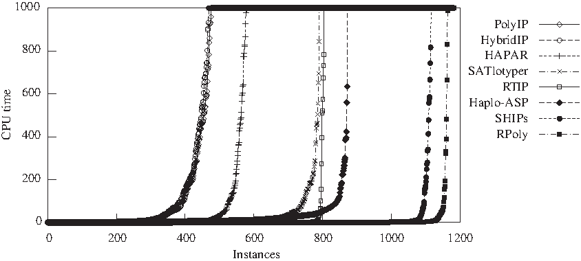
Relative performance of HIPP solvers.

The run times for each solver were sorted and plotted, the cutoff point being 1000 seconds. (This plot format is inspired on the plots traditionally produced with the results of the SAT competition. ¹⁵ ) The memory available was limited to 3 GB. Problem instances on the 1000 seconds horizontal line are instances which exceed the time limit or the memory resources. The plot shows not only the number of problem instances that each approach is able to solve but also the relative performance of each solver. It is clear that the SAT/PBO approaches are significantly more efficient than the other approaches. The best performing solvers, SHIPs and RPoly, are able to trivially solve around 1050 instances. It is also clear from the plot that PolyIP and HybridIP have a very similar performance, followed by HAPAR. RPoly is able to solve more than 98% of the problem instances and SHIPs is able to solve around 94% of the problem instances. HAPLO-ASP solves 74% of the instances, whereas RTIP is able to solve about 68% and SATlotyper solves 67% of the problem instances. The remaining HIPP solvers (HAPAR, PolyIP and HybridIP) have poorer performance, solving less than 50% of the problem instances. Most of the instances aborted by RTIP and HAPLO-ASP are due to memory limitations. HAPLO-ASP and RTIP abort respectively 300 and 299 instances of the phasing class because the memory resources are exceeded.

This section also illustrates the effectiveness of the bounding techniques described in Section 4. For this study, only the instances that have been solved by at least one of the HIPP approaches have been taken into account. (This procedure has eliminated 13 out of the 1183 instances.) Otherwise it would not be possible to compare the values of the computed bounds with the optimal solution.

Figure 12 provides a comparison between the lower bound and the HIPP solution, for the 1170 problem instances whose HIPP solution is known. For around 30% of the instances, the lower bound computes the exact HIPP solution. Moreover, for the majority of the instances (more precisely 83%) the difference between the lower bound and the HIPP solution is less than or equal to 5.

OPEN IN VIEWER

FIG. 12.

Quality of the lower bound.

The evaluation of the upper bound computation is summarized in Figure 13. For 53% of the instances, the upper bound algorithm computes the exact HIPP solution. In addition, for 87% of the instances the difference between the computed upper bound and the HIPP solution is less or equal to 5.

OPEN IN VIEWER

FIG. 13.

Quality of the upper bound.

Finally, Figure 14 compares the lower and upper bound values obtained for each instance. For this plot the whole set of 1183 instances was evaluated. We may observe that for 22% of the instances both values are exactly the same. This means that computing lower and upper bounds suffices to solve these problem instances (i.e., no search is required). In addition, the difference between the upper bound and the lower bound is less or equal to 5 for 70% of the instances and less or equal to 10 for 83% of the instances, thus predictably not requiring much time to be solved.

OPEN IN VIEWER

FIG. 14.

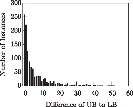
Quality of the bounds.

13. Discussion

A well-known tool for haplotype inference is PHASE (Stephens et al., 2001; Stephens and Donnelly, 2003; Stephens and Scheet, 2005), a statistically-based method following the coalescent approach.

PHASE is known to be an accurate method, although often inefficient, for haplotype inference (Marchini et al., 2006). Accuracy is measured by the correct association between genotypes and explaining haplotypes. Even though it is not possible in general to know the precise solution for the haplotype inference problem, there are a few very well-studied sets of genotypes for which the solution is known. This solution is often obtained using different generations from the same population.

We used a timeout of 10,000 seconds to run the PHASE algorithm on the problem instances described in the previous section. PHASE version 2.1.1 ¹⁶ was used. PHASE was able to solve 976 out of 1183 instances within 10,000 seconds.

Figure 15 provides a comparison between the PHASE solution and the HIPP solution, regarding the number of haplotypes used in the solution. We used the set of 963 problem instances for which the HIPP solution is known and for which PHASE is able to give a solution within 10,000 seconds. For approximately 65% of the instances, the PHASE solution and the HIPP solution are exactly the same (i.e., require the same number of haplotypes). Moreover, for the large majority of the instances (more precisely 88%) the difference between the PHASE solution and the HIPP solution is less than or equal to 5.

OPEN IN VIEWER

FIG. 15.

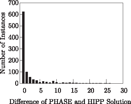
Difference between the PHASE solution and the HIPP solution (number of haplotypes).

In addition, for 34% of the problem instances, the set of haplotypes in the solution provided by the HIPP solver RPoly is exactly the same set of haplotypes provided by PHASE. (This result should be similar using a different HIPP solver because HIPP solvers have no other criterion than parsimony.) Furthermore, on average, 70% of the haplotypes are the same on both the RPoly and PHASE solutions.

This result emphasizes that solutions which tend to be accurate are typically parsimonious or close to parsimonious. However, in general, and for a single instance, the number of solutions satisfying the pure parsimony criterion can be large. The reason for this is that although the HIPP criterion imposes a constraint on the number of haplotypes in the solution, the same set of haplotypes can be used in different ways to explain the genotypes. In addition, there can be solutions with different sets of haplotypes that still have minimum size.

To illustrate this issue, we have performed an extensive evaluation for a specific instance from the phasing class: SU-100kb.25, which has 34 genotypes and 15 sites. The SU-100kb.25 instance has 48 parsimonious solutions with 17 haplotypes each. Fourteen out of 17 haplotypes are common to all HIPP solutions. The remaining 3 haplotypes are picked from a set of 7 haplotypes and are used in general to explain only one genotype. If we compare each pair of HIPP solutions, we observe that out of the 1128 solution pairs, 72 pairs have exactly the same haplotypes, 384 pairs differ in 1 haplotype, 480 pairs differ in 2 haplotypes and 192 pairs differ in 3 haplotypes. Future research directions should consider using a criterion to choose the most accurate solution between all possible HIPP solutions.

14. Conclusions

The relevance of haplotype-association studies with diseases and the significance of missing data imputation reveals the importance of haplotype inference methods. The pure parsimony criterion has been shown in the past to be an accurate approach for haplotype inference (Gusfield, 2003; Wang and Xu, 2003). This problem is NP-hard and consequently a significant number of approaches have been developed to solve the problem efficiently.

This paper presents a survey of haplotype inference by pure parsimony methods including an evaluation of the performance of all exact approaches. The results suggest that the methods based on Boolean satisfiability are significantly more efficient. In particular, the pseudo-Boolean approach RPoly is the method with is able to solve a larger set of instances within a reasonable amount of time.

The computational effectiveness of modern HIPP solvers can make the pure parsimony approach competitive with other more standard haplotype inference approaches. Future work should consider choosing the best HIPP solution taking into account its accuracy.