K-Partite RNA Secondary Structures

Abstract

RNA secondary structure prediction is a fundamental problem in structural bioinformatics. The prediction problem is difficult because RNA secondary structures may contain pseudoknots formed by crossing base pairs. We introduce k-partite secondary structures as a simple classification of RNA secondary structures with pseudoknots. An RNA secondary structure is k-partite if it is the union of k pseudoknot-free sub-structures. Most known RNA secondary structures are either bipartite or tripartite. We show that there exists a constant number k such that any secondary structure can be modified into a k-partite secondary structure with approximately the same free energy. This offers a partial explanation of the prevalence of k-partite secondary structures with small k. We give a complete characterization of the computational complexities of recognizing k-partite secondary structures for all k ≥ 2, and show that this recognition problem is essentially the same as the k-colorability problem on circle graphs. We present two simple heuristics, iterated peeling and first-fit packing, for finding k-partite RNA secondary structures. For maximizing the number of base pair stackings, our iterated peeling heuristic achieves a constant approximation ratio of at most k for 2 ≤ k ≤ 5, and at most \documentclass{aastex}\usepackage{amsbsy}\usepackage{amsfonts}\usepackage{amssymb}\usepackage{bm}\usepackage{mathrsfs}\usepackage{pifont}\usepackage{stmaryrd}\usepackage{textcomp}\usepackage{portland, xspace}\usepackage{amsmath, amsxtra}\pagestyle{empty}\DeclareMathSizes{10}{9}{7}{6}\begin{document}$$\frac {6} {1 - (1 - 6 / k)^k} \le \frac {6} {1 - e^ {- 6}} < 6.01491$$\end {document} for k ≥ 6. Experiment on sequences from PseudoBase shows that our first-fit packing heuristic outperforms the leading method HotKnots in predicting RNA secondary structures with pseudoknots. Supplementary Material can be found at www.libertonline.com.

1. Introduction

The problem of RNA secondary structure prediction is a fundamental issue in structural bioinformatics. The main theme of classical research on this problem has been the design of dynamic programming algorithms that, given an RNA sequence, compute the “optimal” secondary structure of the sequence with the lowest free energy. The first dynamic programming algorithm for predicting pseudoknot-free RNA secondary structures dates back to the 1970s (Nussinov, 1978), and has been implemented by well-known software packages such as Mfold (Zuker, 2003) and Vienna (Hofacker, 2003). During the last decade, several dynamic programming algorithms have also been designed for the much more difficult problem of predicting RNA secondary structures with pseudoknots (Rivas and Eddy, 1999; Uemura et al., 1999; Lyngsø and Pedersen, 2000; Akutsu, 2000; Dirks and Pierce, 2003; Reeder and Giegerich, 2004; Jabbari et al., 2008). These algorithms are often ad-hoc, and can handle only pseudoknots of certain restricted types implicit in their dynamic programming formulations (Condon et al., 2004; Rastegari and Condon, 2007). If arbitrary pseudoknots are allowed in the secondary structures, then the prediction problem becomes computationally intractable even in very simple models (Ieong et al., 2003; Lyngsø, 2004), and we have to resort to approximation algorithms (Jiang, 2009) and heuristics (Ruan et al., 2004; Ren et al., 2005).

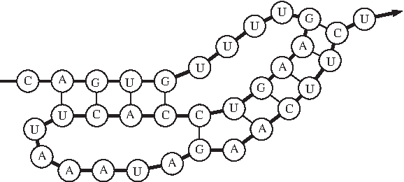
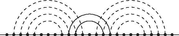
In this article, we study k-partite RNA secondary structures. Intuitively, an RNA secondary structure is k-partite if it is the union of k pseudoknot-free sub-structures. For the k = 2 case, bipartite secondary structures have been previously studied as the bi-secondary structures (Haslinger and Stadler, 1999; Witwer et al., 2004) and the planar secondary structures (Ieong et al., 2003). A recent result on the enumeration of RNA pseudoknots (Rødland, 2006) implies that most known RNA secondary structures are either bipartite or tripartite, i.e., k-partite for k = 2 or 3. Indeed, among the hundreds of known RNA secondary structures with pseudoknots in PseudoBase (van Batenburg et al., 2000), only one structure1 is tripartite, and the others are all bipartite (see Fig. 1 for an example2). The prevalence of bipartite and tripartite secondary structures has motivated us to consider k-partite RNA secondary structures.

FIG. 1.

A bipartite secondary structure.

The main results of this article are the following:

We show that there exists a constant number k such that any secondary structure of an RNA sequence can be modified into a k-partite secondary structure with approximately the same free energy. This offers a partial explanation of the prevalence of k-partite secondary structures with small k.

We give a complete characterization of the computational complexities of recognizing k-partite secondary structures for all k ≥ 2.

We present two simple heuristics, iterated peeling and first-fit packing, for RNA secondary structure prediction. The iterated peeling heuristic achieves the first non-trivial constant approximation ratios for computing k-partite secondary structures with the maximum numbers of base pair stackings. The first-fit packing heuristic outperforms the leading method HotKnots in predicting RNA secondary structures with pseudoknots.

We introduce some preliminaries. The primary structure of an RNA molecule is the sequence of nucleotides (that is, the four different bases A, C, G, and U) in its single-stranded polymer. In its natural state, an RNA molecule folds into a three-dimensional structure by forming hydrogen bonds between non-consecutive bases that are complementary. The three-dimensional arrangement of the atoms in the folded RNA molecule is the tertiary structure; the collection of base pairs in the tertiary structure is the secondary structure. Two bases are complementary if they are either a Watson-Crick pair {A, U} or {G, C}, or a wobble pair {G, U}. A base pair (i, j) formed by two complementary bases with sequence indices i and j must satisfy the hairpin constraint that j − i > 3, that is, they are separated by at least three other bases in the sequence. Two base pairs (i₁, j₁) and (i₂, j₂) are crossing if either i₁ < i₂ < j₁ < j₂ or i₂ < i₁ < j₂ < j₁, are nesting if either i₁ < i₂ < j₂ < j₁ or i₂ < i₁ < j₁ < j₂, and are sequential if either i₁ < j₁ < i₂ < j₂ or i₂ < j₂ < i₁ < j₁. A secondary structure is a set of disjoint base pairs, where each base participates in at most one base pair. Two crossing base pairs form a pseudoknot. A secondary structure is pseudoknot-free if all base pairs in the structure are either nesting or sequential. A base pair stacking is formed by two consecutive base pairs (i, j) and (i + 1, j − 1). A helix (i, j, l), l ≥ 2, is a set of l consecutive base pairs \documentclass{aastex}\usepackage{amsbsy}\usepackage{amsfonts}\usepackage{amssymb}\usepackage{bm}\usepackage{mathrsfs}\usepackage{pifont}\usepackage{stmaryrd}\usepackage{textcomp}\usepackage{portland, xspace}\usepackage{amsmath, amsxtra}\pagestyle{empty}\DeclareMathSizes{10}{9}{7}{6}\begin{document}$$(i,j), (i + 1, j - 1), \ldots , (i + l - 1, j - l + 1)$$\end {document} , forming l − 1 base pair stackings.

2. Prevalence of k-Partite Secondary Structures With Small k

The following proposition partially explains the interesting fact that most real RNA secondary structures are k-partite for a small k:

Proposition 1

There exists a constant number k such that any secondary structure of an RNA sequence can be modified into a k-partite secondary structure with approximately the same free energy.

This proposition is deliberately stated in an imprecise way, considering the diversity and complexity of the many energy models for RNA folding. To make more precise statements with rigorous proofs, we have to restrict our discussion to simple models. In the following theorem, we focus on the simplest energy model in which the free energy of an RNA secondary structure is proportional to its number of Watson-Crick base pairs {A, U} and {G, C}.

Theorem 1

If an RNA sequence has a secondary structure with n Watson-Crick base pairs, then it must also have a 4-partite secondary structure with at least n − 8 Watson-Crick base pairs. Moreover, each part of the 4-partite secondary structure consists of all nesting pairs.

Proof. Let \documentclass{aastex}\usepackage{amsbsy}\usepackage{amsfonts}\usepackage{amssymb}\usepackage{bm}\usepackage{mathrsfs}\usepackage{pifont}\usepackage{stmaryrd}\usepackage{textcomp}\usepackage{portland, xspace}\usepackage{amsmath, amsxtra}\pagestyle{empty}\DeclareMathSizes{10}{9}{7}{6}\begin{document}$${\cal P}$$\end {document} be a set of n Watson-Crick base pairs in a secondary structure. Partition \documentclass{aastex}\usepackage{amsbsy}\usepackage{amsfonts}\usepackage{amssymb}\usepackage{bm}\usepackage{mathrsfs}\usepackage{pifont}\usepackage{stmaryrd}\usepackage{textcomp}\usepackage{portland, xspace}\usepackage{amsmath, amsxtra}\pagestyle{empty}\DeclareMathSizes{10}{9}{7}{6}\begin{document}$${\cal P}$$\end {document} into four subsets \documentclass{aastex}\usepackage{amsbsy}\usepackage{amsfonts}\usepackage{amssymb}\usepackage{bm}\usepackage{mathrsfs}\usepackage{pifont}\usepackage{stmaryrd}\usepackage{textcomp}\usepackage{portland, xspace}\usepackage{amsmath, amsxtra}\pagestyle{empty}\DeclareMathSizes{10}{9}{7}{6}\begin{document}$${\cal P}_{AU}$$\end {document} , \documentclass{aastex}\usepackage{amsbsy}\usepackage{amsfonts}\usepackage{amssymb}\usepackage{bm}\usepackage{mathrsfs}\usepackage{pifont}\usepackage{stmaryrd}\usepackage{textcomp}\usepackage{portland, xspace}\usepackage{amsmath, amsxtra}\pagestyle{empty}\DeclareMathSizes{10}{9}{7}{6}\begin{document}$${\cal P}_{UA}$$\end {document} , \documentclass{aastex}\usepackage{amsbsy}\usepackage{amsfonts}\usepackage{amssymb}\usepackage{bm}\usepackage{mathrsfs}\usepackage{pifont}\usepackage{stmaryrd}\usepackage{textcomp}\usepackage{portland, xspace}\usepackage{amsmath, amsxtra}\pagestyle{empty}\DeclareMathSizes{10}{9}{7}{6}\begin{document}$${\cal P}_{GC}$$\end {document} , and \documentclass{aastex}\usepackage{amsbsy}\usepackage{amsfonts}\usepackage{amssymb}\usepackage{bm}\usepackage{mathrsfs}\usepackage{pifont}\usepackage{stmaryrd}\usepackage{textcomp}\usepackage{portland, xspace}\usepackage{amsmath, amsxtra}\pagestyle{empty}\DeclareMathSizes{10}{9}{7}{6}\begin{document}$${\cal P}_{CG}$$\end {document} of the four different types of base pairs AU, UA, GC, and CG, respectively. Let x be the number of base pairs in \documentclass{aastex}\usepackage{amsbsy}\usepackage{amsfonts}\usepackage{amssymb}\usepackage{bm}\usepackage{mathrsfs}\usepackage{pifont}\usepackage{stmaryrd}\usepackage{textcomp}\usepackage{portland, xspace}\usepackage{amsmath, amsxtra}\pagestyle{empty}\DeclareMathSizes{10}{9}{7}{6}\begin{document}$${\cal P}_{AU} \cup {\cal P}_{UA}$$\end {document} . We next show that \documentclass{aastex}\usepackage{amsbsy}\usepackage{amsfonts}\usepackage{amssymb}\usepackage{bm}\usepackage{mathrsfs}\usepackage{pifont}\usepackage{stmaryrd}\usepackage{textcomp}\usepackage{portland, xspace}\usepackage{amsmath, amsxtra}\pagestyle{empty}\DeclareMathSizes{10}{9}{7}{6}\begin{document}$${\cal P}_{AU}\cup {\cal P}_{UA}$$\end {document} can be transformed into a bipartite secondary structure with at least x − 4 base pairs. Then, a similar transformation for \documentclass{aastex}\usepackage{amsbsy}\usepackage{amsfonts}\usepackage{amssymb}\usepackage{bm}\usepackage{mathrsfs}\usepackage{pifont}\usepackage{stmaryrd}\usepackage{textcomp}\usepackage{portland, xspace}\usepackage{amsmath, amsxtra}\pagestyle{empty}\DeclareMathSizes{10}{9}{7}{6}\begin{document}$${\cal P}_{GC} \cup {\cal P}_{CG}$$\end {document} completes the proof.

We first consider the subset \documentclass{aastex}\usepackage{amsbsy}\usepackage{amsfonts}\usepackage{amssymb}\usepackage{bm}\usepackage{mathrsfs}\usepackage{pifont}\usepackage{stmaryrd}\usepackage{textcomp}\usepackage{portland, xspace}\usepackage{amsmath, amsxtra}\pagestyle{empty}\DeclareMathSizes{10}{9}{7}{6}\begin{document}$${\cal P}_{AU}$$\end {document} . Let (i₁, j₁) and (i₂, j₂) be the two farthest non-nesting pairs in \documentclass{aastex}\usepackage{amsbsy}\usepackage{amsfonts}\usepackage{amssymb}\usepackage{bm}\usepackage{mathrsfs}\usepackage{pifont}\usepackage{stmaryrd}\usepackage{textcomp}\usepackage{portland, xspace}\usepackage{amsmath, amsxtra}\pagestyle{empty}\DeclareMathSizes{10}{9}{7}{6}\begin{document}$${\cal P}_{AU}$$\end {document} such that the index i₁ is the smallest and the index j₂ is the largest. Then the base pairs (i, j) with i < i₁ or j > j₂ must be nesting, and the other base pairs, including (i₁, j₁) and (i₂, j₂), are nested inside them. If j₂ − i₁ > 3, we swap the two non-nesting pairs into two nesting pairs as in Figure 2: (a) if (i₁, j₁) and (i₂, j₂) are sequential, swap them to two nesting pairs (i₁, j₂) and (j₁, i₂); (b) if (i₁, j₁) and (i₂, j₂) are crossing, swap them to two nesting pairs (i₁, j₂) and (i₂, j₁). In either case, the outer one of the two nesting pairs, (i₁, j₂), is a valid base pair that satisfies the hairpin constraint. In case (a), the inner one of the two nesting pairs is a UA pair, so we move it from \documentclass{aastex}\usepackage{amsbsy}\usepackage{amsfonts}\usepackage{amssymb}\usepackage{bm}\usepackage{mathrsfs}\usepackage{pifont}\usepackage{stmaryrd}\usepackage{textcomp}\usepackage{portland, xspace}\usepackage{amsmath, amsxtra}\pagestyle{empty}\DeclareMathSizes{10}{9}{7}{6}\begin{document}$${\cal P}_{AU}$$\end {document} to \documentclass{aastex}\usepackage{amsbsy}\usepackage{amsfonts}\usepackage{amssymb}\usepackage{bm}\usepackage{mathrsfs}\usepackage{pifont}\usepackage{stmaryrd}\usepackage{textcomp}\usepackage{portland, xspace}\usepackage{amsmath, amsxtra}\pagestyle{empty}\DeclareMathSizes{10}{9}{7}{6}\begin{document}$${\cal P}_{UA}$$\end {document} . Define this swap operation similarly for \documentclass{aastex}\usepackage{amsbsy}\usepackage{amsfonts}\usepackage{amssymb}\usepackage{bm}\usepackage{mathrsfs}\usepackage{pifont}\usepackage{stmaryrd}\usepackage{textcomp}\usepackage{portland, xspace}\usepackage{amsmath, amsxtra}\pagestyle{empty}\DeclareMathSizes{10}{9}{7}{6}\begin{document}$${\cal P}_{UA}$$\end {document} .

FIG. 2.
(a) Swap two sequential base pairs to two nesting pairs. (b) Swap two crossing base pairs to two nesting pairs.

Each base pair (i, j) has a pair distance j − i. The x pairs in \documentclass{aastex}\usepackage{amsbsy}\usepackage{amsfonts}\usepackage{amssymb}\usepackage{bm}\usepackage{mathrsfs}\usepackage{pifont}\usepackage{stmaryrd}\usepackage{textcomp}\usepackage{portland, xspace}\usepackage{amsmath, amsxtra}\pagestyle{empty}\DeclareMathSizes{10}{9}{7}{6}\begin{document}$${\cal P}_{AU} \cup {\cal P}_{UA}$$\end {document} correspond to x pair distances, which can be sorted in non-ascending order to a distance vector of x fields. In either case (a) or case (b) of the swap operation, the larger one of the two pair distances always increases after the swap, thus the distance vector of the x pairs in \documentclass{aastex}\usepackage{amsbsy}\usepackage{amsfonts}\usepackage{amssymb}\usepackage{bm}\usepackage{mathrsfs}\usepackage{pifont}\usepackage{stmaryrd}\usepackage{textcomp}\usepackage{portland, xspace}\usepackage{amsmath, amsxtra}\pagestyle{empty}\DeclareMathSizes{10}{9}{7}{6}\begin{document}$${\cal P}_{AU} \cup {\cal P}_{UA}$$\end {document} always increases lexicographically. Since each pair distance is at least 1 and at most n − 1, the total number of different distance vectors is at most (n − 1)^x, which is a finite number. Repeat the swap operation on the two subsets \documentclass{aastex}\usepackage{amsbsy}\usepackage{amsfonts}\usepackage{amssymb}\usepackage{bm}\usepackage{mathrsfs}\usepackage{pifont}\usepackage{stmaryrd}\usepackage{textcomp}\usepackage{portland, xspace}\usepackage{amsmath, amsxtra}\pagestyle{empty}\DeclareMathSizes{10}{9}{7}{6}\begin{document}$${\cal P}_{AU}$$\end {document} and \documentclass{aastex}\usepackage{amsbsy}\usepackage{amsfonts}\usepackage{amssymb}\usepackage{bm}\usepackage{mathrsfs}\usepackage{pifont}\usepackage{stmaryrd}\usepackage{textcomp}\usepackage{portland, xspace}\usepackage{amsmath, amsxtra}\pagestyle{empty}\DeclareMathSizes{10}{9}{7}{6}\begin{document}$${\cal P}_{UA}$$\end {document} whenever possible. Eventually, after at most (n − 1)^x swap operations, each subset consists of all nesting base pairs except for at most two pairs in the middle that may not satisfy the hairpin constraint and are discarded. We have thus transformed \documentclass{aastex}\usepackage{amsbsy}\usepackage{amsfonts}\usepackage{amssymb}\usepackage{bm}\usepackage{mathrsfs}\usepackage{pifont}\usepackage{stmaryrd}\usepackage{textcomp}\usepackage{portland, xspace}\usepackage{amsmath, amsxtra}\pagestyle{empty}\DeclareMathSizes{10}{9}{7}{6}\begin{document}$${\cal P}_{AU} \cup {\cal P}_{UA}$$\end {document} into a bipartite secondary structure with at least x − 4 base pairs. A similar transformation for \documentclass{aastex}\usepackage{amsbsy}\usepackage{amsfonts}\usepackage{amssymb}\usepackage{bm}\usepackage{mathrsfs}\usepackage{pifont}\usepackage{stmaryrd}\usepackage{textcomp}\usepackage{portland, xspace}\usepackage{amsmath, amsxtra}\pagestyle{empty}\DeclareMathSizes{10}{9}{7}{6}\begin{document}$${\cal P}_{GC} \cup {\cal P}_{CG}$$\end {document} completes the proof. ▪

We note that the number n − 8 in Theorem 1 is not optimized and can be improved to at least n − 4 by a tighter analysis. On the other hand, if we want to keep the same number n of base pairs in the k-partite secondary structure, then the number k = 4 in Theorem 1 is best possible, as we can see from the sequence AUGCUACG with 4 crossing base pairs (1, 5), (2, 6), (3, 7), and (4, 8).

We next consider a more realistic model in which the free energy of an RNA secondary structure is proportional to the total length of its helices, i.e., the total number of stacking base pairs. Assume again for simplicity that only Watson-Crick pairs are allowed in the helices. Recall that a helix must have length at least 2. Then any helix of length l ≥ 4 can be decomposed into ⌊l/2⌋ short helices of lengths 2 and 3. Since there are 4² different doubles and 4³ different triples of RNA bases, any secondary structure can be partitioned into at most 4² + 4³ = 80 subsets, and every two subsets of complementary bases can be transformed into a bipartite secondary structure as we did for \documentclass{aastex}\usepackage{amsbsy}\usepackage{amsfonts}\usepackage{amssymb}\usepackage{bm}\usepackage{mathrsfs}\usepackage{pifont}\usepackage{stmaryrd}\usepackage{textcomp}\usepackage{portland, xspace}\usepackage{amsmath, amsxtra}\pagestyle{empty}\DeclareMathSizes{10}{9}{7}{6}\begin{document}$${\cal P}_{AU}$$\end {document} and \documentclass{aastex}\usepackage{amsbsy}\usepackage{amsfonts}\usepackage{amssymb}\usepackage{bm}\usepackage{mathrsfs}\usepackage{pifont}\usepackage{stmaryrd}\usepackage{textcomp}\usepackage{portland, xspace}\usepackage{amsmath, amsxtra}\pagestyle{empty}\DeclareMathSizes{10}{9}{7}{6}\begin{document}$${\cal P}_{UA}$$\end {document} in the proof of Theorem 1. Thus, Proposition 1 remains valid for this model.

3. Recognizing k-Partite Secondary Structures

Any RNA sequence of bases can be represented by a circular sequence of points on a circle such that two bases consecutive in the RNA sequence correspond to two points consecutive on the circle. Then each base pair of a secondary structure can be represented by a chord in the circle connecting the two corresponding points. The intersection graph of n chords in a circle is a circle graph of n vertices, one vertex for each chord. Two vertices are adjacent in the circle graph if and only if the two corresponding chords intersect, that is, if and only if the two corresponding base pairs cross. Thus the problem of recognizing k-partite secondary structures is equivalent to the problem of deciding whether a circle graph (given the explicit chord representation) has a k-coloring. Indeed, the two problems can be reduced to each other in linear time.

The equivalence of an RNA secondary structure and a circle graph implies the following charaterization of k-partite secondary structures: A secondary structure is k-partite if and only if its corresponding circle graph has chromatic number at most k. We note here a related concept called k-noncrossing secondary structures,3 which are defined as secondary structures containing no more than k mutually crossing base pairs (Huang et al., 2008). In terms of circle graphs, we have the following charaterization: A secondary structure is k-noncrossing if and only if its corresponding circle graph has clique number at most k. Recall that a circle graph is not a perfect graph, thus in general the chromatic number and the clique number of a circle graph are not equal.

We now proceed to the recognition of k-partite secondary structures using the charaterization based on circle graphs. It is known that coloring circle graphs is NP-complete (Garey et al., 1980). Moreover, for any constant k ≥ 4, deciding whether a circle graph has a k-coloring is also NP-complete (Unger, 1988). For k = 3, the 3-coloring problem admits an O(n log n) time algorithm given the explicit representation of n chords (Unger, 1992). For k = 2, the 2-coloring problem is the same as the problem of testing bipartiteness4 of circle graphs. It is well known that bipartiteness testing, even for general graphs, admits a linear-time algorithm (linear in the total number of vertices and edges) (Kleinberg and Tardos, 2005). But since a circle graph of n vertices can have as many as \documentclass{aastex}\usepackage{amsbsy}\usepackage{amsfonts}\usepackage{amssymb}\usepackage{bm}\usepackage{mathrsfs}\usepackage{pifont}\usepackage{stmaryrd}\usepackage{textcomp}\usepackage{portland, xspace}\usepackage{amsmath, amsxtra}\pagestyle{empty}\DeclareMathSizes{10}{9}{7}{6}\begin{document}$$\bigg (\begin{matrix}{n}\\{2}\end{matrix} \bigg)$$\end {document} edges, a straight-forward application of the generic linear-time algorithm for bipartiteness testing gives only an O(n²) time algorithm for the 2-coloring of circle graphs.

An alternative way to obtain an O(n²) time algorithm for the 2-coloring problem is to encode the circle graph as a 2-SAT formula: the color of each chord corresponds to the true/false value of a boolean variable; two crossing chords of variables x₁ and x₂ correspond to two clauses \documentclass{aastex}\usepackage{amsbsy}\usepackage{amsfonts}\usepackage{amssymb}\usepackage{bm}\usepackage{mathrsfs}\usepackage{pifont}\usepackage{stmaryrd}\usepackage{textcomp}\usepackage{portland, xspace}\usepackage{amsmath, amsxtra}\pagestyle{empty}\DeclareMathSizes{10}{9}{7}{6}\begin{document}$$x_1 \vee x_2$$\end {document} and \documentclass{aastex}\usepackage{amsbsy}\usepackage{amsfonts}\usepackage{amssymb}\usepackage{bm}\usepackage{mathrsfs}\usepackage{pifont}\usepackage{stmaryrd}\usepackage{textcomp}\usepackage{portland, xspace}\usepackage{amsmath, amsxtra}\pagestyle{empty}\DeclareMathSizes{10}{9}{7}{6}\begin{document}$$\neg x_1 \vee \neg x_2$$\end {document} . Since 2-SAT also admits a linear-time algorithm (Aspvall et al., 1979), we again have an O(n²) time algorithm for the 2-coloring of circle graphs.

A circle graph is the intersection graph of a set of chords in a circle. In general, we can have intersection graphs of arbitrary line segments in the plane. The 2-coloring problem for circle graphs is thus a special case of the problem of testing bipartiteness of segment intersection graphs. Recently, Eppstein (2004) designed a rather sophisticated O(n log n) time algorithm for this general problem, given the explicit representation of n segments. This immediately implies an O(n log n) time algorithm for the 2-coloring of circle graphs. We are not aware of any simple algorithm for the 2-coloring of circle graphs that runs in o(n²) time and is easy to implement.

We summarize the results in the following theorem:

Theorem 2

Recognizing k-partite secondary structures is NP-complete for any constant k ≥ 4, and admits O(n log n) time algorithms for k = 2 and 3, where n is the number of base pairs in the input secondary structure.

4. Iterated Peeling

A k-partite secondary structure consists of k disjoint pseudoknot-free sub-structures. We now present an iterated peeling heuristic that, given a sequence S of RNA bases, extracts k disjoint sub-structures one by one in a greedy fashion as follows. First find a pseudoknot-free structure \documentclass{aastex}\usepackage{amsbsy}\usepackage{amsfonts}\usepackage{amssymb}\usepackage{bm}\usepackage{mathrsfs}\usepackage{pifont}\usepackage{stmaryrd}\usepackage{textcomp}\usepackage{portland, xspace}\usepackage{amsmath, amsxtra}\pagestyle{empty}\DeclareMathSizes{10}{9}{7}{6}\begin{document}$${\cal P}_1$$\end {document} with the lowest energy of the given sequence. Next find a pseudoknot-free structure \documentclass{aastex}\usepackage{amsbsy}\usepackage{amsfonts}\usepackage{amssymb}\usepackage{bm}\usepackage{mathrsfs}\usepackage{pifont}\usepackage{stmaryrd}\usepackage{textcomp}\usepackage{portland, xspace}\usepackage{amsmath, amsxtra}\pagestyle{empty}\DeclareMathSizes{10}{9}{7}{6}\begin{document}$${\cal P}_2$$\end {document} with the lowest energy of the subsequence of bases that are not paired up in \documentclass{aastex}\usepackage{amsbsy}\usepackage{amsfonts}\usepackage{amssymb}\usepackage{bm}\usepackage{mathrsfs}\usepackage{pifont}\usepackage{stmaryrd}\usepackage{textcomp}\usepackage{portland, xspace}\usepackage{amsmath, amsxtra}\pagestyle{empty}\DeclareMathSizes{10}{9}{7}{6}\begin{document}$${\cal P}_1$$\end {document} . In general, at step t, find a pseudoknot-free structure \documentclass{aastex}\usepackage{amsbsy}\usepackage{amsfonts}\usepackage{amssymb}\usepackage{bm}\usepackage{mathrsfs}\usepackage{pifont}\usepackage{stmaryrd}\usepackage{textcomp}\usepackage{portland, xspace}\usepackage{amsmath, amsxtra}\pagestyle{empty}\DeclareMathSizes{10}{9}{7}{6}\begin{document}$${\cal P}_t$$\end {document} with the lowest energy of the subsequence of bases that are not paired up in any previous structure \documentclass{aastex}\usepackage{amsbsy}\usepackage{amsfonts}\usepackage{amssymb}\usepackage{bm}\usepackage{mathrsfs}\usepackage{pifont}\usepackage{stmaryrd}\usepackage{textcomp}\usepackage{portland, xspace}\usepackage{amsmath, amsxtra}\pagestyle{empty}\DeclareMathSizes{10}{9}{7}{6}\begin{document}$${\cal P}_s$$\end {document} , 1 ≤ s ≤ t − 1. After k steps, return the k-partite secondary structure \documentclass{aastex}\usepackage{amsbsy}\usepackage{amsfonts}\usepackage{amssymb}\usepackage{bm}\usepackage{mathrsfs}\usepackage{pifont}\usepackage{stmaryrd}\usepackage{textcomp}\usepackage{portland, xspace}\usepackage{amsmath, amsxtra}\pagestyle{empty}\DeclareMathSizes{10}{9}{7}{6}\begin{document}$${\cal P}_1 \cup \cdots \cup {\cal P}_k$$\end {document} .

Since the stackings of base pairs contribute the most to the overall free energy of a secondary structure, we use dynamic programming at each step of the iterated peeling heuristic to find a pseudoknot-free sub-structure with the minimum stacking energy. Our dynamic programming algorithm is similar in spirit to an algorithm by Ieong et al. (2003), but the latter does not distinguish the bases yet unpaired from the bases already paired up at the previous steps, and has the optimization goal of maximizing the (positive) number of base pair stackings instead of minimizing the (negative) stacking energy.

We now describe the dynamic programming algorithm. Denote by W(i, j) the lowest stacking energy of a pseudoknot-free secondary structure of the subsequence S[i, j]. Denote by V (i, j) the lowest stacking energy of a pseudoknot-free secondary structure of the subsequence S[i, j] with the additional constraint that the two bases i and j must either form a base pair or do not participate in any base pairs at all. Let E₂(i, j, i + 1, j − 1) be the stacking energy of the two pairs (i, j) and (i + 1, j − 1) if none of the four bases i, j, i + 1, j − 1 are paired at the previous steps, and let it be + ∞ otherwise. Recall that any base pair (i, j) must satisfy the hairpin constraint j − i ≥ 4. The base case and the recurrence of the dynamic programming algorithm are as follows:

Base case: For all (i, j) such that i ≤ j ≤ i + 4, \documentclass{aastex}\usepackage{amsbsy}\usepackage{amsfonts}\usepackage{amssymb}\usepackage{bm}\usepackage{mathrsfs}\usepackage{pifont}\usepackage{stmaryrd}\usepackage{textcomp}\usepackage{portland, xspace}\usepackage{amsmath, amsxtra}\pagestyle{empty}\DeclareMathSizes{10}{9}{7}{6}\begin{document}$$W (i, j) = V (i, j) = 0.$$\end {document}

Recurrence: For all (i, j) such that j ≥ i + 5, \documentclass{aastex}\usepackage{amsbsy}\usepackage{amsfonts}\usepackage{amssymb}\usepackage{bm}\usepackage{mathrsfs}\usepackage{pifont}\usepackage{stmaryrd}\usepackage{textcomp}\usepackage{portland, xspace}\usepackage{amsmath, amsxtra}\pagestyle{empty}\DeclareMathSizes{10}{9}{7}{6}\begin{document}\begin{align}V (i, j) = \min & \bigg \{W (i + 1, j - 1) , V (i + 1, j - 1) + E_2 (i, j, i + 1, j - 1) \bigg \}, \\ & \ W (i, j) = \min \left\{V (i, j) , \min_{i \le x < j} \{W (i, x) + W (x + 1, j) \} \right\} .\end{align}\end {document}

To recover the secondary structure of the lowest stacking energy, we need another table X(i, j) to store the choices of decomposition. During the computation of two tables V (i, j) and W(i, j), if W(i, j) is W(i, x) + W(x + 1, j) for some index x, then set X(i, j) to this index x. Otherwise W(i, j) is V (i, j), which is the smaller of the two values W(i + 1, j − 1) and V (i + 1, j − 1) + E₂(i, j, i + 1, j − 1). These two values correspond to the two cases that (i) the two bases i and j are both unpaired and (ii) the base pair (i, j) stacks with the base pair (i + 1, j − 1). Set X(i, j) to −1 in case (i), and to −2 in case (ii).

After the computation of the three tables V (i, j), W(i, j), and X(i, j), we recover the optimal secondary structure for S[1, n] using a recursive procedure that marks the paired bases. For a subsequence S[i, j] with a negative stacking energy W(i, j), the recursive procedure considers three cases:
If X[i, j] = −2, continue marking the bases i + c and j − c for \documentclass{aastex}\usepackage{amsbsy}\usepackage{amsfonts}\usepackage{amssymb}\usepackage{bm}\usepackage{mathrsfs}\usepackage{pifont}\usepackage{stmaryrd}\usepackage{textcomp}\usepackage{portland, xspace}\usepackage{amsmath, amsxtra}\pagestyle{empty}\DeclareMathSizes{10}{9}{7}{6}\begin{document}$$c = 0, 1, 2, \ldots , c^$$\end {document} until X[i + c][j − c] ≠−2, then mark the subsequence S[i + c + 1, j − c* − 1] recursively.

If X[i, j] = −1, mark the subsequence S[i + 1, j − 1] recursively.

Otherwise, let x = X[i, j]. Mark the two subsequences S[i, x] and S[x + 1, j] recursively.

The dynamic programming algorithm clearly runs in O(ℓ³) time, where ℓ is the sequence length. Thus the overall running time of the iterated peeling heuristic is O(kℓ³). We next analyze the approximation ratio of the iterated peeling heuristic. For simplicity, we consider the unweighted version of the problem that maximizes the number of base pair stackings (that is, with an energy of −1 for each base pair stacking, minimizes the stacking energy). Ieong et al. (2003) have shown that the problem of finding a bipartite secondary structure with the maximum number of base pair stackings is NP-complete and admits a 2-approximation.

Let \documentclass{aastex}\usepackage{amsbsy}\usepackage{amsfonts}\usepackage{amssymb}\usepackage{bm}\usepackage{mathrsfs}\usepackage{pifont}\usepackage{stmaryrd}\usepackage{textcomp}\usepackage{portland, xspace}\usepackage{amsmath, amsxtra}\pagestyle{empty}\DeclareMathSizes{10}{9}{7}{6}\begin{document}$${\cal S}^$$\end {document} be an optimal k-partite secondary structure with the maximum number N of base pair stackings. By the Pigeon-hole principle, at least one of the k pseudoknot-free sub-structures of \documentclass{aastex}\usepackage{amsbsy}\usepackage{amsfonts}\usepackage{amssymb}\usepackage{bm}\usepackage{mathrsfs}\usepackage{pifont}\usepackage{stmaryrd}\usepackage{textcomp}\usepackage{portland, xspace}\usepackage{amsmath, amsxtra}\pagestyle{empty}\DeclareMathSizes{10}{9}{7}{6}\begin{document}$${\cal S}^$$\end {document} has at most \documentclass{aastex}\usepackage{amsbsy}\usepackage{amsfonts}\usepackage{amssymb}\usepackage{bm}\usepackage{mathrsfs}\usepackage{pifont}\usepackage{stmaryrd}\usepackage{textcomp}\usepackage{portland, xspace}\usepackage{amsmath, amsxtra}\pagestyle{empty}\DeclareMathSizes{10}{9}{7}{6}\begin{document}$$N^ / k$$\end {document} base pair stackings. Let n_s be the number of base pair stackings in the sub-structure \documentclass{aastex}\usepackage{amsbsy}\usepackage{amsfonts}\usepackage{amssymb}\usepackage{bm}\usepackage{mathrsfs}\usepackage{pifont}\usepackage{stmaryrd}\usepackage{textcomp}\usepackage{portland, xspace}\usepackage{amsmath, amsxtra}\pagestyle{empty}\DeclareMathSizes{10}{9}{7}{6}\begin{document}$${\cal P}_s$$\end {document} obtained at step s of the heuristic. Then \documentclass{aastex}\usepackage{amsbsy}\usepackage{amsfonts}\usepackage{amssymb}\usepackage{bm}\usepackage{mathrsfs}\usepackage{pifont}\usepackage{stmaryrd}\usepackage{textcomp}\usepackage{portland, xspace}\usepackage{amsmath, amsxtra}\pagestyle{empty}\DeclareMathSizes{10}{9}{7}{6}\begin{document}$$\sum\nolimits_{s = 1}^{k} n_s \geq n_1 \geq N^* / k$$\end {document} , that is, even the first step of the heuristic alone already achieves a k-approximation. By Proposition 1, the optimal k-partite secondary structure \documentclass{aastex}\usepackage{amsbsy}\usepackage{amsfonts}\usepackage{amssymb}\usepackage{bm}\usepackage{mathrsfs}\usepackage{pifont}\usepackage{stmaryrd}\usepackage{textcomp}\usepackage{portland, xspace}\usepackage{amsmath, amsxtra}\pagestyle{empty}\DeclareMathSizes{10}{9}{7}{6}\begin{document}$${\cal S}^$$\end {document} , even for a potentially unbounded number k, can be modified into a k′-partite secondary structure \documentclass{aastex}\usepackage{amsbsy}\usepackage{amsfonts}\usepackage{amssymb}\usepackage{bm}\usepackage{mathrsfs}\usepackage{pifont}\usepackage{stmaryrd}\usepackage{textcomp}\usepackage{portland, xspace}\usepackage{amsmath, amsxtra}\pagestyle{empty}\DeclareMathSizes{10}{9}{7}{6}\begin{document}$${\cal S}^ \prime$$\end {document} with approximately the same free energy, such that k′ is a constant. Thus the heuristic indeed achieves a constant approximation even for arbitrary k. We next show, without using the implication of Proposition 1, that the iterated peeling heuristic still achieves a small constant approximation for arbitrary k. For this we need to consider the contributions n_s* by the subsequent steps \documentclass{aastex}\usepackage{amsbsy}\usepackage{amsfonts}\usepackage{amssymb}\usepackage{bm}\usepackage{mathrsfs}\usepackage{pifont}\usepackage{stmaryrd}\usepackage{textcomp}\usepackage{portland, xspace}\usepackage{amsmath, amsxtra}\pagestyle{empty}\DeclareMathSizes{10}{9}{7}{6}\begin{document}$$s = 2, \ldots , k$$\end {document} . The idea of our analysis comes from the analysis of a similar heuristic for multi-layer routing in integrated circuit layout design (Cong et al., 1993). In the following, we consider only the case that k ≥ 6 since the approximation ratio of k achieved by the first step of the heuristic is already quite small for 2 ≤ k ≤ 5.

Consider an arbitrary base pair stacking found by the iterated peeling heuristic. If this stacking is not in the optimal structure \documentclass{aastex}\usepackage{amsbsy}\usepackage{amsfonts}\usepackage{amssymb}\usepackage{bm}\usepackage{mathrsfs}\usepackage{pifont}\usepackage{stmaryrd}\usepackage{textcomp}\usepackage{portland, xspace}\usepackage{amsmath, amsxtra}\pagestyle{empty}\DeclareMathSizes{10}{9}{7}{6}\begin{document}$${\cal S}^$$\end {document} , then it intersects at most 6 stackings in \documentclass{aastex}\usepackage{amsbsy}\usepackage{amsfonts}\usepackage{amssymb}\usepackage{bm}\usepackage{mathrsfs}\usepackage{pifont}\usepackage{stmaryrd}\usepackage{textcomp}\usepackage{portland, xspace}\usepackage{amsmath, amsxtra}\pagestyle{empty}\DeclareMathSizes{10}{9}{7}{6}\begin{document}$${\cal S}^$$\end {document} (Fig. 3). Thus, by the Pigeon-hole principle, we have the following inequalities:
FIG. 3.
One base pair stacking intersects six other base pair stackings.
\documentclass{aastex}\usepackage{amsbsy}\usepackage{amsfonts}\usepackage{amssymb}\usepackage{bm}\usepackage{mathrsfs}\usepackage{pifont}\usepackage{stmaryrd}\usepackage{textcomp}\usepackage{portland, xspace}\usepackage{amsmath, amsxtra}\pagestyle{empty}\DeclareMathSizes{10}{9}{7}{6}\begin{document}\begin{align}n_1 & \ge \frac {N^} {k} \\ n_2 & \ge \frac {N^* - 6n_1} {k} \\ n_3 & \ge \frac {N^* - 6 (n_1 + n_2)} {k} \\ &\hspace{3pt} \vdots \\ n_k & \ge \frac {N^ - 6 (n_1 + \cdots + n_{k - 1})} {k} \end{align}\end {document}

Let \documentclass{aastex}\usepackage{amsbsy}\usepackage{amsfonts}\usepackage{amssymb}\usepackage{bm}\usepackage{mathrsfs}\usepackage{pifont}\usepackage{stmaryrd}\usepackage{textcomp}\usepackage{portland, xspace}\usepackage{amsmath, amsxtra}\pagestyle{empty}\DeclareMathSizes{10}{9}{7}{6}\begin{document}\begin{align}x_1 & = \frac {N^} {k} \\ x_2 & = \frac {N^ - 6x_1} {k} \\ x_3 & = \frac {N^* - 6 (x_1 + x_2)} {k} \\ &\hspace{3pt} \vdots \\ x_k & = \frac {N^ - 6 (x_1 + \cdots + x_ {k - 1})} {k} \end{align}\end {document}

We now prove that \documentclass{aastex}\usepackage{amsbsy}\usepackage{amsfonts}\usepackage{amssymb}\usepackage{bm}\usepackage{mathrsfs}\usepackage{pifont}\usepackage{stmaryrd}\usepackage{textcomp}\usepackage{portland, xspace}\usepackage{amsmath, amsxtra}\pagestyle{empty}\DeclareMathSizes{10}{9}{7}{6}\begin{document}$$\sum\nolimits_{s = 1}^t n_s \geq \sum\nolimits_{s = 1}^t x_s$$\end {document} for 1 ≤ t ≤ k by induction. The base case n₁ ≥ x₁ for t = 1 is obvious. For the inductive step from t to t + 1, we have (for k ≥ 6) \documentclass{aastex}\usepackage{amsbsy}\usepackage{amsfonts}\usepackage{amssymb}\usepackage{bm}\usepackage{mathrsfs}\usepackage{pifont}\usepackage{stmaryrd}\usepackage{textcomp}\usepackage{portland, xspace}\usepackage{amsmath, amsxtra}\pagestyle{empty}\DeclareMathSizes{10}{9}{7}{6}\begin{document}\begin{align} \sum_ {s = 1}^ {t + 1} n_s & \ge \sum_ {s = 1}^t n_s + \frac {N^* - 6 \sum \limits_ {s = 1}^t n_s} {k} \quad = \frac {N^* + (k - 6) \sum \limits_{s = 1}^t n_s} {k} \\ & \ge \frac {N^* + (k - 6) \sum \limits_ {s = 1}^t x_s} {k} = \sum_ {s = 1}^t x_s + \frac {N^* - 6 \sum \limits_{s = 1}^t x_s} {k} = \sum_{s = 1}^ {t + 1} x_s. \end{align}\end {document}

It remains to bound \documentclass{aastex}\usepackage{amsbsy}\usepackage{amsfonts}\usepackage{amssymb}\usepackage{bm}\usepackage{mathrsfs}\usepackage{pifont}\usepackage{stmaryrd}\usepackage{textcomp}\usepackage{portland, xspace}\usepackage{amsmath, amsxtra}\pagestyle{empty}\DeclareMathSizes{10}{9}{7}{6}\begin{document}$$\sum\nolimits_{s = 1}^k x_s$$\end {document} in terms of N. Note that k(x_s − x_s₋₁) = − 6x_s₋₁ for 2 ≤ s ≤ k. Thus \documentclass{aastex}\usepackage{amsbsy}\usepackage{amsfonts}\usepackage{amssymb}\usepackage{bm}\usepackage{mathrsfs}\usepackage{pifont}\usepackage{stmaryrd}\usepackage{textcomp}\usepackage{portland, xspace}\usepackage{amsmath, amsxtra}\pagestyle{empty}\DeclareMathSizes{10}{9}{7}{6}\begin{document}\begin{align}x_s = (1 - \frac {6} {k}) x_ {s - 1} = \cdots = (1 - \frac {6} {k})^ {s - 1} x_1.\end{align}\end {document}

It follows that \documentclass{aastex}\usepackage{amsbsy}\usepackage{amsfonts}\usepackage{amssymb}\usepackage{bm}\usepackage{mathrsfs}\usepackage{pifont}\usepackage{stmaryrd}\usepackage{textcomp}\usepackage{portland, xspace}\usepackage{amsmath, amsxtra}\pagestyle{empty}\DeclareMathSizes{10}{9}{7}{6}\begin{document}\begin{align}\sum_ {s = 1}^k x_s = x_1 \cdot \sum_ {s = 1}^k \left(1 - \frac {6} {k} \right)^ {s - 1} = \frac {N^} {k} \cdot \frac {1 - (1 - 6 / k)^k} {1 - (1 - 6 / k)} = \frac {1 - (1 - 6 / k)^k} {6} \cdot N^.\end{align}\end {document}

Note that \documentclass{aastex}\usepackage{amsbsy}\usepackage{amsfonts}\usepackage{amssymb}\usepackage{bm}\usepackage{mathrsfs}\usepackage{pifont}\usepackage{stmaryrd}\usepackage{textcomp}\usepackage{portland, xspace}\usepackage{amsmath, amsxtra}\pagestyle{empty}\DeclareMathSizes{10}{9}{7}{6}\begin{document}\begin{align}(1 - 6 / k)^k = ((1 - 6 / k)^{k / 6})^6 \le (\lim_{x \to \infty} (1 - 1 / x)^x)^6 = (1 / e)^6.\end{align}\end {document}

Thus, the approximation ratio of the iterated peeling heuristic is \documentclass{aastex}\usepackage{amsbsy}\usepackage{amsfonts}\usepackage{amssymb}\usepackage{bm}\usepackage{mathrsfs}\usepackage{pifont}\usepackage{stmaryrd}\usepackage{textcomp}\usepackage{portland, xspace}\usepackage{amsmath, amsxtra}\pagestyle{empty}\DeclareMathSizes{10}{9}{7}{6}\begin{document}\begin{align} \frac {N^} {\sum_ {s = 1}^k n_s} \le \frac {N^} {\sum_ {s = 1}^k x_s} = \frac {6} {1 - (1 - 6 / k)^k} \le \frac {6} {1 - e^ {- 6}} = 6.014909 \ldots.\end{align}\end {document}

We have proved the following theorem:

Theorem 3

Given an RNA sequence of length ℓ, the iterated peeling heuristic finds a k-partite secondary structure in O(kℓ³) time. The approximation ratio of the heuristic for maximizing the number of base pair stackings is at most k for 2 ≤ k ≤ 5, and is at most \documentclass{aastex}\usepackage{amsbsy}\usepackage{amsfonts}\usepackage{amssymb}\usepackage{bm}\usepackage{mathrsfs}\usepackage{pifont}\usepackage{stmaryrd}\usepackage{textcomp}\usepackage{portland, xspace}\usepackage{amsmath, amsxtra}\pagestyle{empty}\DeclareMathSizes{10}{9}{7}{6}\begin{document}$$ \frac {6} {1 - (1 - 6 / k)^k} \le \frac {6} {1 - e^ {- 6}} < 6.01491$$\end {document} for k ≥ 6.

5. First-Fit Packing

The iterated peeling heuristic discussed in the previous section uses the greedy approach to find k sub-structures that compose a k-partite secondary structure. We now present another heuristic that applies the greedy approach in an entirely different way. Our first-fit packing heuristic is based on the first-fit strategy for the classical combinatorial optimization problem of multiple knapsack packing. Intuitively, the k sub-structures are the k knapsacks, and each helix of at least two stacking base pairs is an item to be packed into one of the knapsacks; the helices (items) in each sub-structure (knapsack) must be disjoint and non-crossing.

The first-fit packing heuristic runs in four steps: first extract base pairs from the sequence, next group the stacking base pairs into helices, then extend each helix until maximal, and finally select a disjoint set of base pairs from the helices.

To extract base pairs from the sequence, we use a simple criterion: If two stacking base pairs (i, j) and (i + 1, j − 1) are both Watson-Crick pairs, then both base pairs are extracted. If a base pair (i, j) is a wobble pair and is stacked with two other base pairs (i − 1, j + 1) and (i + 1, j − 1) that are both Watson-Crick pairs, then all three base pairs are extracted.

Consecutive base pairs are grouped into helices. We do not allow bulges or internal loops in the helices. Thus each helix consists exclusively of stacking base pairs, and can be specified by three numbers (i, j, l), where (i, j) is the outer-most base pair in the helix, and l is the helix length, i.e., the number of base pairs in the helix. For example, the helix (4, 12, 3) consists of three stacking base pairs (4, 12), (5, 11), and (6, 10). The extraction of base pairs and the grouping of stacking base pairs into helices can be accomplished at the same time by a simple dynamic programming algorithm in O(ℓ²) time, where ℓ is the sequence length.

We then extend each helix into a maximal helix. First extend (i, j, l) inward to (i, j, l + c) incrementally, for \documentclass{aastex}\usepackage{amsbsy}\usepackage{amsfonts}\usepackage{amssymb}\usepackage{bm}\usepackage{mathrsfs}\usepackage{pifont}\usepackage{stmaryrd}\usepackage{textcomp}\usepackage{portland, xspace}\usepackage{amsmath, amsxtra}\pagestyle{empty}\DeclareMathSizes{10}{9}{7}{6}\begin{document}$$c = 1, 2, \ldots$$\end {document} , while the inner-most base pair satisfies the hairpin constraint (j − l − c + 1) − (i + l + c − 1) > 3 and the helix energy becomes lower. Next extend the helix outward, from (i, j, l′) to (i − c, j + c,l′ + c), in a similar manner.

Finally, we select a disjoint set of base pairs from these maximal helices. This is done by repeating the following selection round until every candidate helix is either discarded, or added to a sub-structure \documentclass{aastex}\usepackage{amsbsy}\usepackage{amsfonts}\usepackage{amssymb}\usepackage{bm}\usepackage{mathrsfs}\usepackage{pifont}\usepackage{stmaryrd}\usepackage{textcomp}\usepackage{portland, xspace}\usepackage{amsmath, amsxtra}\pagestyle{empty}\DeclareMathSizes{10}{9}{7}{6}\begin{document}$${\cal P}_s$$\end {document} , 1 ≤ s ≤ k:
Find a helix H with the lowest stacking energy among the candidate helices not yet added to any sub-structure.

Find the sub-structure \documentclass{aastex}\usepackage{amsbsy}\usepackage{amsfonts}\usepackage{amssymb}\usepackage{bm}\usepackage{mathrsfs}\usepackage{pifont}\usepackage{stmaryrd}\usepackage{textcomp}\usepackage{portland, xspace}\usepackage{amsmath, amsxtra}\pagestyle{empty}\DeclareMathSizes{10}{9}{7}{6}\begin{document}$${\cal P}_s$$\end {document} with the smallest index s such that H does not cross any helices already in \documentclass{aastex}\usepackage{amsbsy}\usepackage{amsfonts}\usepackage{amssymb}\usepackage{bm}\usepackage{mathrsfs}\usepackage{pifont}\usepackage{stmaryrd}\usepackage{textcomp}\usepackage{portland, xspace}\usepackage{amsmath, amsxtra}\pagestyle{empty}\DeclareMathSizes{10}{9}{7}{6}\begin{document}$${\cal P}_s$$\end {document} .

If no such sub-structure \documentclass{aastex}\usepackage{amsbsy}\usepackage{amsfonts}\usepackage{amssymb}\usepackage{bm}\usepackage{mathrsfs}\usepackage{pifont}\usepackage{stmaryrd}\usepackage{textcomp}\usepackage{portland, xspace}\usepackage{amsmath, amsxtra}\pagestyle{empty}\DeclareMathSizes{10}{9}{7}{6}\begin{document}$${\cal P}_s$$\end {document} exists, discard the helix H. Otherwise, add H to \documentclass{aastex}\usepackage{amsbsy}\usepackage{amsfonts}\usepackage{amssymb}\usepackage{bm}\usepackage{mathrsfs}\usepackage{pifont}\usepackage{stmaryrd}\usepackage{textcomp}\usepackage{portland, xspace}\usepackage{amsmath, amsxtra}\pagestyle{empty}\DeclareMathSizes{10}{9}{7}{6}\begin{document}$${\cal P}_s$$\end {document} , then trim all remaining candidate helices such that their base pairs that overlap with H are removed. If a candidate helix is shortened to less than three base pairs after the trimming, discard it.

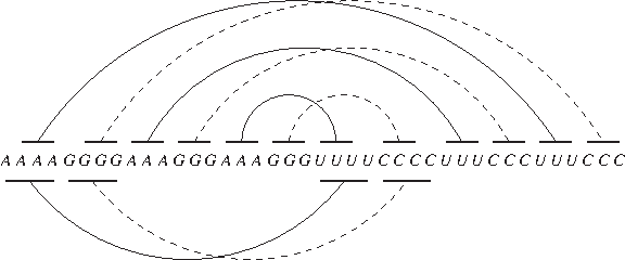
The first-fit packing heuristic and the iterated peeling heuristic are both based on the greedy approach. But the first-fit packing heuristic, unlike the iterated peeling heuristic, does not seem to achieve any constant approximation ratio for maximizing the number of base pair stackings. When k = 2, for example, the sequence A⁴G⁴(A³G³)^rU⁴C⁴(U³C³)^r has an optimal bipartite secondary structure of 4r + 4 stackings, but the first-fit packing heuristic finds only 6 stackings (see Fig. 4 for an illustration where r = 2). Nevertheless, as we will show in the next section, the first-fit packing heuristic beats the iterated peeling heuristic in predicting RNA secondary structures.

FIG. 4.
An example for finding bipartite secondary structures. (Upper) The optimal structure. (Lower) The structure found by the first-fit packing heuristic. The two sub-structures of each bipartite secondary structure are depicted by solid and dashed arcs respectively.

6. Experiment on RNA Secondary Structure Prediction

We compare our two greedy heuristics, code-named IPeel for iterated peeling and FPack for first-fit packing, with the HotKnots algorithm of Ren et al. (2005) on RNA secondary structure prediction. HotKnots is a leading method for RNA secondary structure prediction that has been shown to outperform the well-known Pseudoknots algorithm of Rivas and Eddy (1999), the NUPACK algorithm of Dirks and Pierce (2003), and the Iterated Loop Matching algorithm of Ruan et al. (2004), and to give better results in many cases than the genetic algorithm from the STAR package of van Batenburg et al. (1995) and the pknotsRG-mfe algorithm of Reeder and Giegerich (2004).

For the test data, we use the RNA sequences with known secondary structures from PseudoBase (van Batenburg et al., 2000). As of May 25, 2008, the PseudoBase contained 279 partial RNA sequences, of which 252 are consecutive sequences without gaps. We collected these 252 sequences and their known secondary structures (in dot-bracket format) in a FASTA file pseudobase.fasta as the data set. The sequences in the data set have maximum length 131 and minimum length 20; the average length is about 43 with a standard deviation of 24.

For each sequence in the data set, we use each of the three methods, HotKnots, IPeel, and FPack, to predict a secondary structure, then compare the predicted secondary structures with the known secondary structure from PseudoBase. The parameter k is set to 2 for our methods IPeel and FPack. The three methods are all very efficient; the entire experiment finishes in less than four minutes on an Apple iMac with 2 GHz PowerPC G5 Processor and 2 GB RAM running Mac OS X 10.4.11.

To compare a predicted secondary structure with a known secondary structure, we count the true positives as the base pairs that are known and are predicted, the false negatives as the base pairs that are known but are not predicted, and the false positives as the base pairs that are not known but are predicted. Then we define three quality measures: \documentclass{aastex}\usepackage{amsbsy}\usepackage{amsfonts}\usepackage{amssymb}\usepackage{bm}\usepackage{mathrsfs}\usepackage{pifont}\usepackage{stmaryrd}\usepackage{textcomp}\usepackage{portland, xspace}\usepackage{amsmath, amsxtra}\pagestyle{empty}\DeclareMathSizes{10}{9}{7}{6}\begin{document}\begin{align} {\rm Sensitivity} & = \frac {\# \ {\rm true \ positives}} {\# \ {\rm true \ positives} + \# \ {\rm false \ negatives}} \\ {\rm Selectivity} & = \frac {\# \ {\rm true \ positives}} {\# \ {\rm true \ positives} + \# \ {\rm false \ negatives}} \\ {\rm Accuracy} & = \frac {\# \ {\rm true \ positives}} {\# \ {\rm true \ positives} + \# \ {\rm false \ negatives} + \# \ {\rm false \ positives}} \end{align}\end {document}

Both sensitivity and selectivity are standard quality measures that are widely used. We introduce the measure of accuracy here as a combination of sensitivity and selectivity. Intuitively, consider the predicted secondary structure and the known secondary structure as two sets of base pairs, then the measure of accuracy corresponds to the intersection of the two sets over the union of the two sets.

To compare the overall performances of the three methods (HotKnots, IPeel, and FPack), we calculate the three quality measures (sensitivity, selectivity, and accuracy) of each method using the equations above with the three numbers (true positives, false negatives, and false positives) summed over all 252 sequences in the data set. We obtained the following results:

Sensitivity Selectivity Accuracy

HotKnots 71.69% 78.47% 59.90%

IPeel 51.09% 42.33% 30.12%

FPack 80.50% 75.39% 63.75%

The results are a little surprising. The iterated peeling heuristic is the most theoretically interesting among the three methods, but it has the worst performance in this experiment. On the other hand, although not achieving any constant approximation ratio, the first-fit packing heuristic performs the best. Note that FPack is slightly worse than HotKnots in selectivity but outperforms HotKnots in both sensitivity and accuracy. It is impressive that a rather simple (indeed almost naive) greedy method can have such a good performance. Our explanation for this unexpected success is the following:
For RNA folding, the kinetic aspect of the folding process is as important as the thermodynamic stability of the folded structure.

For the simulation of RNA folding kinetics, the greedy choice of selecting helices one by one (first-fit packing) is more realistic than the greedy choice of selecting sub-structures one by one (iterated peeling).

7. Supplementary Material

Our RNA folding programs have been tested on three major platforms: Windows (Cygwin on XP), Linux (Ubunta), and Mac OS X. The complete source code, data set, and experimental results can be received as Supplementary Material at www.liebertonline.com.

	Sensitivity	Selectivity	Accuracy
HotKnots	71.69%	78.47%	59.90%
IPeel	51.09%	42.33%	30.12%
FPack	80.50%	75.39%	63.75%

Footnotes

Acknowledgments

This work is supported in part by NSF (grant DBI-0743670). An abstract of this work was presented at the 9th Workshop on Algorithms in Bioinformatics (WABI’09) and appears in the workshop proceedings.

Disclosure Statement

No competing financial interests exist.

1

PKB00071: pseudoknot of regulatory region of alpha ribosomal protein operon of E. coli.

2

PKB00116: pseudoknot PKb of upstream pseudoknot domain of 3′-UTR of beet soil-borne virus RNA 1.

3

We thank an anonymous referee of WABI’09 for bringing to our attention this very recent work of Reidys's group.

4

Haslinger and Stadler (1999, Theorem 2(vi)) incorrectly characterized this problem as testing the triangle-free property. Note that the five base pairs (1, 5), (3, 7), (6, 10), (8, 12), and (2, 11) induce a 5-cycle in the circle graph, which is triangle-free but not bipartite. Indeed, Ageev () even constructed a triangle-free circle graph with chromatic number 5.

References

Ageev

A.A.

1996. A triangle-free circle graph with chromatic number 5. Discrete Math, 152:295–298.

Akutsu

2000. Dynamic programming algorithms for RNA secondary structure prediction with pseudoknots. Discrete Appl. Math., 104:45–62.

Aspvall

, Plass

M.F.

, Tarjan

R.E.

1979. A linear-time algorithm for testing the truth of certain quantified boolean formulas. Inform. Process. Lett., 8:121–123.

Batenburg van

F.H.D.

, Gultyaev

A.P.

, Pleij

C.W.A.

1995. An APL-programmed genetic algorithm for the prediction of RNA secondary structure. J. Theoret. Biol., 174:269–280.

Batenburg van

F.H.D.

, Gultyaev

A.P.

, Pleij

C.W.A.

et al. 2000. Pseudobase: a database with RNA pseudoknots. Nucleic Acids Res., 28:201–204.

Chung

F.R.K.

, Leighton

F.T.

, Rosenberg

A.L.

1987. Embedding graphs in books: a layout problem with applications to VLSI design. SIAM J. Algebraic Discrete Methods, 8:33–58.

Condon

, Davy

, Rastegari

et al. 2004. Classifying RNA pseudoknotted structures. Theoret Comput Sci., 320:35–50.

Cong

, Hossain

, Sherwani

N.A.

1993. A provably good multilayer topological planar routing algorithms in IC layout designs. IEEE Trans Comput. Aided Design Integrated Circuits Syst., 12:70–78.

Dirks

R.M.

, Pierce

N.A.

2003. A partition function algorithm for nucleic acid secondary structure including pseudoknots. J. Comput. Chem., 24:1664–1677.

10.

Eppstein

2004. Testing bipartiteness of geometric intersection graphs. Proc. SODA’04, 860–868.

11.

Garey

M.R.

, Johnson

D.S.

, Miller

G.L.

et al. 1980. The complexity of coloring circular arcs and chords. SIAM J. Algebraic Discrete Methods, 1:216–227.

12.

Haslinger

, Stadler

P.F.

1999. RNA structures with pseudo-knots: graph theoretical, combinatorial, and statistical properties. Bull. Math. Biol., 61:437–467.

13.

Hofacker

I.L.

2003. Vienna RNA secondary structure server. Nucleic Acids Res., 31:3429–3431.

14.

Huang

F.W.D.

, Peng

W.W.J.

, Reidys

C.M.

2008. Folding 3-noncrossing RNA pseudoknot structures. http://arxiv.org/abs/0809.4840v1. 2010 May 1.

15.

Ieong

, Kao

M.-Y.

, Lam

T.-W.

et al. 2003. Predicting RNA secondary structure with arbitrary pseudoknots by maximizing the number of stacking pairs. J. Comput. Biol., 10:981–995.

16.

Jabbari

, Condon

, Zhao

2008. Novel and efficient RNA secondary structure prediction using hierarchical folding. J. Comput. Biol., 15:139–163.

17.

Jiang

2009. Approximation algorithms for predicting RNA secondary structures with arbitrary pseudoknots. ACM/IEEE Trans. Comput. Biol. Bioinform. http://dx.doi.org/10.1109/TCBB.2008.109. 2010 May 1.

18.

Kleinberg

, Tardos

2005. Algorithm Design. Addison Wesley: New York.

19.

Lyngsø

R.B.

2004. Complexity of pseudoknot prediction in simple models. Proc. ICALP’04, 919–931.

20.

Lyngsø

R.B.

, Pedersen

C.N.S.

2000. RNA pseudoknot prediction in energy-based models. J. Computat. Biol., 7:409–427.

21.

Mathews

D.H.

, Sabina

, Zuker

et al. 1999. Expanded sequence dependence of thermodynamic parameters improves prediction of RNA secondary structure. J. Mol. Biol., 288:911–940.

22.

Nussinov

, Pieczenik

, Griggs

J.R.

et al. 1978. Algorithms for loop matching. SIAM J. Appl. Math., 35:68–82.

23.

Rastegari

, Condon

2007. Parsing nucleic acid pseudoknotted secondary structure: algorithm and applications. J. Comput. Biol., 14:16–32.

24.

Reeder

, Giegerich

2004. Design, implementation and evaluation of a practical pseudoknot folding algorithm based on thermodynamics. BMC Bioinform., 5:104.

25.

Ren

, Rastegari

, Condon

et al. 2005. HotKnots: heuristic prediction of RNA secondary structures including pseudoknots. RNA, 11:1494–1504.

26.

Rivas

, Eddy

S.R.

1999. A dynamic programming algorithm for RNA structure prediction including pseudoknots. J. Mol. Biol., 285:2053–2068.

27.

Rødland

E.A.

2006. Pseudoknots in RNA secondary structures: representation, enumeration, and prevalence. J. Comput. Biol., 13:1197–1213.

28.

Ruan

, Stormo

G.D.

, Zhang

2004. An iterated loop matching approach to the prediction of RNA secondary structure with pseudoknots. Bioinformatics, 20:58–66.

29.

Tinoco

, Borer

P.N.

, Dengler

et al. 1973. Improved estimation of secondary structure in ribonucleic acids. Nat. New Biol., 246:40–42.

30.

Uemura

, Hasegawa

, Kobayashi

et al. 1999. Tree adjoining grammars for RNA structure prediction. Theoret. Comput. Sci., 210:277–303.

31.

Unger

1988. On the k-colouring of circle-graphs. Lect. Notes Comput. Sci., 294:61–72.

32.

Unger

1992. The complexity of colouring circle graphs. Lect. Notes Comput. Sci., 577:389–400.

33.

Witwer

, Hofacker

I.L.

, Stadler

P.F.

2004. Prediction of consensus RNA secondary structures including pseudoknots. IEEE/ACM Trans. Comput. Biol. Bioinform., 1:66–77.

34.

Zuker

2003. Mfold web server for nucleic acid folding and hybridization prediction. Nucleic Acids Res., 31:3406–3415.

Supplementary Material

Please find the following supplemental material available below.

For Open Access articles published under a Creative Commons License, all supplemental material carries the same license as the article it is associated with.

For non-Open Access articles published, all supplemental material carries a non-exclusive license, and permission requests for re-use of supplemental material or any part of supplemental material shall be sent directly to the copyright owner as specified in the copyright notice associated with the article.

0.19 MB

0.00 MB