Feature Detection with Controlled Error Rates in LC/MS Images

Abstract

The Median M-N rule is a feature detection algorithm to detect peptide signals in Liquid Chromatography/Mass Spectrometry (LC/MS) images. As the procedure does not adequately control the statistical errors, we investigate an extension of the Median M-N rule to compute a statistical bound on the false-positive rate. We then study the false-negative rate and provide insights on the types of signal that can be detected by the M-N rule and the limit of detection. The resulting feature detection algorithm, which we term Quantile M-N rule, can be used in most feature detection algorithms to provide statistical control of the false-positive and false-negative rate. Supplementary Material is available at www.liebertonline.com/cmb.

1. Introduction

The large-scale analysis of the proteome is fostering the development of new high-throughput methodologies in mass spectrometry. While many types of mass spectrometers as well as sample handling protocols are available, the current trend is to digest the proteins with proteases such as trypsin, fractionate the resulting mixture of peptides using liquid-chromatography (LC) columns, then analyse each fraction using a mass spectrometer (Aebersold and Mann, 2003; Simpson and Smith, 2005; Domon and Aebersold, 2006).

When the sample enters the mass spectrometer, the molecules are ionised, accelerated and the instrument records the intensity of the resulting ion beam in a range of mass-to-charge values. This first-stage experiment produces mass spectrometry (MS) spectra. However, current technologies are not sufficient to identify all the peptides that are present in a complex sample (Aebersold and Mann, 2003). Peptides (and hence proteins) are usually identified by a subsequent second-stage experiment which breaks the amino acid chain between the residues and produces fragmentation spectra (also called MS/MS or tandem MS spectra) (MacCoss, 2005). Many methods and algorithms for interpreting these fragmentation spectra are available, either de novo (Frank et al., 2007) or starting from a reference database containing the relevant/potential proteins—Sequest (Eng et al., 1994) and Mascot (Perkins et al., 1999). For a review, see Sadygov et al. (2004).

Although the above MS/MS approach is now mainstream and has provided many results, there is interest in analyzing MS spectra. For example, the retention time and mass-to-charge location of a signal may be sufficient to identify the corresponding peptide sequence, as has been demonstrated in the AMT approach by Smith et al. (2002). Due to reproducibility issues, however, this kind of procedure currently relies on high-precision instrumentation and tightly controlled LC elution (Norbeck et al., 2005; Vandenbogaert et al., 2008).

The MS spectra also represent the primary source of quantitative measures (Bantscheff et al., 2007), although alternatives approaches are gaining ground (ITRAQ [Wiese et al., 2007] and MRM [Kitteringham et al., 2008]). Last, but not least, the acquisition of MS/MS spectra is a major bottleneck in high-throughput analyses; not performing the time-consuming MS/MS fragmentation can provide a significant decrease in instrument time.

The present article examines a preprocessing algorithm to enhance the analysis of MS spectra acquired on LC/MS platforms. Prior to identification and quantification, peptide signals need to be extracted from the dataset, (i.e., a list of features of interest needs to be built). This consists of two steps, usually implemented in the same software. First, the LC/MS data is quickly scanned for candidate signals. Then more computationally intensive procedures (“template matching”) are used to precisely quantify diverse characteristics of each feature such as m/z value, retention time, charge state, and area under the curve. For a survey of available methods and software), see Yang et al. (2009).

Current approaches for candidate selection are mostly based on local maxima, either in the measured intensity (Yasui et al., 2003; Tibshirani et al., 2004; Noy and Fasulo, 2007; Kalousis et al., 2005; Mantini et al., 2007; Wang et al., 2006; Yu et al., 2006; Katajamaa and Oresic, 2005) or in the wavelet transform of the signal (Randolph and Yasui, 2006; Lange et al., 2006; Bellew et al., 2006; Tautenhahn et al., 2008; Morris et al., 2005; Noy and Fasulo, 2007). In both cases, local maxima contain high numbers of false positives, and the list of candidates is filtered based on signal-to-noise ratio (Morris et al., 2005; Noy and Fasulo, 2007; Mantini et al., 2007; Wang et al., 2006), peak width (Yu et al., 2006; Katajamaa and Oresic, 2005), or based on the reproducible presence of the peak in adjacent MS spectra (Kalousis et al., 2005; Mantini et al., 2007; Wang et al., 2006). The approach presented by Radulovic et al. (2004), which we will here call Median M-N rule, does not require the candidate to be a local maximum, but focuses on high-intensity peaks that appear in consecutive MS scans.

For accurate determination of the peak characteristics and especially the m/z ratio of the peak centroid, most methods match a template to the observed intensity values. There are several models available for individual peaks, including double Gaussian functions (Kempka et al., 2004; Strittmatter et al., 2003; Leptos et al., 2006), asymmetric Lorentzian or sech functions (Lange et al., 2006), and exponentially modified Gaussian functions (Naish and Hartwell, 1988; Jin et al., 2008; Li, 2002). However, the template approach is best used to match the patterns of peaks created by isotopes (Noy and Fasulo, 2007; Gras et al., 1999; Jaitly et al., 2004).

As indicated by Du et al. (2006), the performance of feature detection directly affects the subsequent processes, such as retention time alignment (Jeffries, 2005), protein identification (Rejtar et al., 2004), and biomarker identification (Li et al., 2005). However, due to the complexity of the signals and multiple sources of noise in MS spectra, high false-positive peak identification rate is a major problem, especially in detecting peaks with low amplitudes (Hilario et al., 2006).

Candidate selection drives the performance of feature detection in terms of sensitivity and selectivity whereas the second step determines the precision of identification and quantification. Among the various possibilities, we evaluate the Median M-N rule (Radulovic et al., 2004) as a candidate selection algorithm because it is computationally efficient and also amenable to statistical analysis. We first show that the original formulation allows a limited level of control of the false-positive rate. To improve upon this, we present an extended M-N rule and compute its statistical properties. We first compute the false-positive rate and propose guidelines to improve the number of true positives. We then demonstrate its application to an experimental data set.

Supplementary Material is available at www.liebertonline.com/cmb.

2. Methods

2.1. Feature detection with the Median M-N rule

Radulovic et al. (2004) present the following feature detection algorithm. A peptide signal is detected by the Median M-N rule if the intensity in N consecutive MS spectra exceeds the threshold M × C where C is 30% of the trimmed mean or the median. The authors claim that the parameters (M = 3, N = 3) can be used in many different contexts with low false-positive rate.

When applying the Median M-N rule, we have observed that the false-positive rate may depend on the m/z value (Fig. 1). This suggests that the false-positive rate in the Median M-N rule is not well controlled. Consequently, the algorithm may provide an unspecified number of undesirable entries in the peak list, which may result in false identifications and wrong biomarkers. We defer the details of the estimation of the false-positive rate to Section 3.4 because it builds on concepts and hypotheses provided in the rest of this section.

FIG. 1.

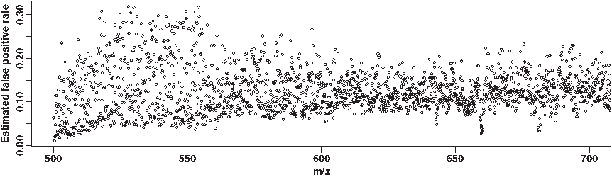
False-positive rate in Radulovic et al. (2004). The data set and the estimation procedure are described in Sections 3.1 and 3.4.

2.2. Extended M-N rule

In this article, we propose the following generalization of the M-N rule. A peptide is detected by the extended M-N rule if the intensity in N consecutive scans exceeds the threshold H. The Median M-N rule in Radulovic et al. (2004) corresponds to using the threshold H = M × C. In Section 2.5, we will present an alternative choice for H, which we call the Quantile M-N rule, and show how it improves the control of the false-positive rate.

In Radulovic et al. (2004), the Median M-N rule adapts to local noise characteristics, although the parameters M and N are fixed for the entire data set. This is because the actual threshold H = M × C is a function of retention time and m/z through the median noise intensity C(t, m). The extended formulation allows H to be an arbitrary function H(t, m) of the position in the LC/MS image.

2.3. LC/MS data model

Computing the statistical properties of the detector requires a model of the signal generated on the LC/MS platform (described in this section) and procedures to estimate the model parameters (described in Section 3.2). We assume that the measured intensity \documentclass{aastex}\usepackage{amsbsy}\usepackage{amsfonts}\usepackage{amssymb}\usepackage{bm}\usepackage{mathrsfs}\usepackage{pifont}\usepackage{stmaryrd}\usepackage{textcomp}\usepackage{portland, xspace}\usepackage{amsmath, amsxtra}\pagestyle{empty}\DeclareMathSizes{10}{9}{7}{6}\begin{document} $${\cal I} (t, m)$$ \end{document} is the sum of a random noise component \documentclass{aastex}\usepackage{amsbsy}\usepackage{amsfonts}\usepackage{amssymb}\usepackage{bm}\usepackage{mathrsfs}\usepackage{pifont}\usepackage{stmaryrd}\usepackage{textcomp}\usepackage{portland, xspace}\usepackage{amsmath, amsxtra}\pagestyle{empty}\DeclareMathSizes{10}{9}{7}{6}\begin{document} $${\cal N} (t, m)$$ \end{document} and an independent and deterministic peptide signal component \documentclass{aastex}\usepackage{amsbsy}\usepackage{amsfonts}\usepackage{amssymb}\usepackage{bm}\usepackage{mathrsfs}\usepackage{pifont}\usepackage{stmaryrd}\usepackage{textcomp}\usepackage{portland, xspace}\usepackage{amsmath, amsxtra}\pagestyle{empty}\DeclareMathSizes{10}{9}{7}{6}\begin{document} $${\cal S} (t, m)$$ \end{document} .

Both the Median M-N rule and the extended M-N rule only take into account intensity in the same m/z bin; we will therefore drop the variable m and write \documentclass{aastex}\usepackage{amsbsy}\usepackage{amsfonts}\usepackage{amssymb}\usepackage{bm}\usepackage{mathrsfs}\usepackage{pifont}\usepackage{stmaryrd}\usepackage{textcomp}\usepackage{portland, xspace}\usepackage{amsmath, amsxtra}\pagestyle{empty}\DeclareMathSizes{10}{9}{7}{6}\begin{document} $${\cal I} (t) = {\cal N} (t) + {\cal S} (t)$$ \end{document} . This is equivalent to analysing the LC/MS data line by line.

As we analyze each m/z bin independently, a model for the m/z separation is not necessary. In the following, we describe the standard model for chromatography elution profiles presented in Snyder et al. (1997) and a model for the background noise process \documentclass{aastex}\usepackage{amsbsy}\usepackage{amsfonts}\usepackage{amssymb}\usepackage{bm}\usepackage{mathrsfs}\usepackage{pifont}\usepackage{stmaryrd}\usepackage{textcomp}\usepackage{portland, xspace}\usepackage{amsmath, amsxtra}\pagestyle{empty}\DeclareMathSizes{10}{9}{7}{6}\begin{document} $${\cal N} (t)$$ \end{document} . To simplify the notations, we will hereafter write M-N rule instead of extended M-N rule, and study the generic properties of this feature detection algorithm.

2.3.1. Elution profile model

In the linear model of chromatography, each peptide produces a Gaussian-shaped elution profile (Snyder et al., 1997; Felinger, 1998). This model has also been used to generate synthetic LC/MS images (Schulz-Trieglaff et al., 2008). We assume that in each m/z bin, the signal \documentclass{aastex}\usepackage{amsbsy}\usepackage{amsfonts}\usepackage{amssymb}\usepackage{bm}\usepackage{mathrsfs}\usepackage{pifont}\usepackage{stmaryrd}\usepackage{textcomp}\usepackage{portland, xspace}\usepackage{amsmath, amsxtra}\pagestyle{empty}\DeclareMathSizes{10}{9}{7}{6}\begin{document} $${\cal S} (t)$$ \end{document} is a superposition of Gaussian profiles, with different retention time and standard deviation. More explicitly: \documentclass{aastex}\usepackage{amsbsy}\usepackage{amsfonts}\usepackage{amssymb}\usepackage{bm}\usepackage{mathrsfs}\usepackage{pifont}\usepackage{stmaryrd}\usepackage{textcomp}\usepackage{portland, xspace}\usepackage{amsmath, amsxtra}\pagestyle{empty}\DeclareMathSizes{10}{9}{7}{6}\begin{document} \begin{align*} {\cal I} (t) = {\cal N} (t) + \sum_k \Gamma_k (t) \end{align*} \end{document}

where Γ_k(t) is the Gaussian trace of peptide k in the current m/z bin, and the sum iterates over the peptides that have a trace in the bin.

Each Gaussian profile Γ_k(t) is a positive real function of the chromatography time \documentclass{aastex}\usepackage{amsbsy}\usepackage{amsfonts}\usepackage{amssymb}\usepackage{bm}\usepackage{mathrsfs}\usepackage{pifont}\usepackage{stmaryrd}\usepackage{textcomp}\usepackage{portland, xspace}\usepackage{amsmath, amsxtra}\pagestyle{empty}\DeclareMathSizes{10}{9}{7}{6}\begin{document} \begin{align*} \Gamma_k (t) = A_k \frac {1} {\sqrt {2 \pi \sigma_k^2}} \exp \left(- \frac {(t - \mu_k)^2} {2 \sigma_k^2} \right) \end{align*} \end{document}

where μ_k is the retention time of peptide k and the parameters σ_k and A_k represent the standard deviation of the profile and its area under the curve respectively. In particular, in LC/MS experiments, A_k is commonly assumed to be proportional to the concentration of peptide k in the sample.

In the standard model, the physical processes in distillation columns lead to the following relation between retention time and standard deviation: \documentclass{aastex}\usepackage{amsbsy}\usepackage{amsfonts}\usepackage{amssymb}\usepackage{bm}\usepackage{mathrsfs}\usepackage{pifont}\usepackage{stmaryrd}\usepackage{textcomp}\usepackage{portland, xspace}\usepackage{amsmath, amsxtra}\pagestyle{empty}\DeclareMathSizes{10}{9}{7}{6}\begin{document} \begin{align*} \sigma_k = \mu_k / \sqrt{P} \tag{1} \end{align*} \end{document}

where P is the plate number of the column. P measures the separation power of the chromatography; the elution profile is tighter (σ_k smaller) with increased values of P.

The plate number is commonly used to describe other types of columns, including those used in LC/MS experiments. However, the use of solvent gradients may invalidate Equation (1) by modulating the retention of peptides on the LC column (μ_k) or the degree of separation (σ_k) during the course of the chromatography. Therefore, we do not use Equation (1) and we expect different possible values for σ_k.

2.3.2. Background noise model

Most methods dealing with background noise in LC/MS images attempt to remove it from the data using with various mathematical tools: wavelets (Coombes et al., 2005; Zhu et al., 2003a; Qu et al., 2003), Fourier transform (Kast et al., 2003), local noise statistics (Satten et al., 2004; Williams et al., 2005), and time series analysis (Andreev et al., 2003; Liu et al., 2003; Howard et al., 2003; Zhu et al., 2003b; Malyarenko et al., 2005). However, removing background noise is difficult because chemical noise produces patterns that are similar to real signals (Andreev et al., 2003). For example, noise patterns are known to have a 1-Da periodicity similar to isotope patterns (Piening et al., 2006).

To control the false-positive rate in feature detection, we use the a contrario detection approach from image analysis introduced in Desolneux et al. (2000, 2001). This approach is based on detecting image features as exceptional configurations in random images. As such, it requires that the noise characteristics be known a priori or estimated from the image. Several models for the background noise distribution in LC/MS images have previously been proposed (Anderle et al., 2004; Hastings et al., 2002; Wallace et al., 2004; Shin et al., 2007) but are difficult to use in a contrario detection.

Instead of detailed modeling of the background noise, we use few hypotheses so that the approach remains generic. We simply assume that the random noise is an independent process and that all the pixels in the same horizontal line have the same distribution. Consequently, we will write \documentclass{aastex}\usepackage{amsbsy}\usepackage{amsfonts}\usepackage{amssymb}\usepackage{bm}\usepackage{mathrsfs}\usepackage{pifont}\usepackage{stmaryrd}\usepackage{textcomp}\usepackage{portland, xspace}\usepackage{amsmath, amsxtra}\pagestyle{empty}\DeclareMathSizes{10}{9}{7}{6}\begin{document} $${\cal N}$$ \end{document} instead of \documentclass{aastex}\usepackage{amsbsy}\usepackage{amsfonts}\usepackage{amssymb}\usepackage{bm}\usepackage{mathrsfs}\usepackage{pifont}\usepackage{stmaryrd}\usepackage{textcomp}\usepackage{portland, xspace}\usepackage{amsmath, amsxtra}\pagestyle{empty}\DeclareMathSizes{10}{9}{7}{6}\begin{document} $${\cal N} (t)$$ \end{document} . This requires that the LC/MS data is normalized beforehand, but greatly eases the practical estimation of local noise characteristics.

2.4. Statistical testing framework

Let us define a pamphlet of width N as a series of N intensity values \documentclass{aastex}\usepackage{amsbsy}\usepackage{amsfonts}\usepackage{amssymb}\usepackage{bm}\usepackage{mathrsfs}\usepackage{pifont}\usepackage{stmaryrd}\usepackage{textcomp}\usepackage{portland, xspace}\usepackage{amsmath, amsxtra}\pagestyle{empty}\DeclareMathSizes{10}{9}{7}{6}\begin{document} $$({\cal I} (t_1, m), \ldots, {\cal I} (t_N, m))$$ \end{document} measured at the same m/z ratio m in consecutive MS spectra obtained at the retention times \documentclass{aastex}\usepackage{amsbsy}\usepackage{amsfonts}\usepackage{amssymb}\usepackage{bm}\usepackage{mathrsfs}\usepackage{pifont}\usepackage{stmaryrd}\usepackage{textcomp}\usepackage{portland, xspace}\usepackage{amsmath, amsxtra}\pagestyle{empty}\DeclareMathSizes{10}{9}{7}{6}\begin{document} $$(t_1, \ldots, t_N)$$ \end{document} . In the following, we will use the notation \documentclass{aastex}\usepackage{amsbsy}\usepackage{amsfonts}\usepackage{amssymb}\usepackage{bm}\usepackage{mathrsfs}\usepackage{pifont}\usepackage{stmaryrd}\usepackage{textcomp}\usepackage{portland, xspace}\usepackage{amsmath, amsxtra}\pagestyle{empty}\DeclareMathSizes{10}{9}{7}{6}\begin{document} $${\cal I} (t_i, m) = {\cal I}_i$$ \end{document} for all \documentclass{aastex}\usepackage{amsbsy}\usepackage{amsfonts}\usepackage{amssymb}\usepackage{bm}\usepackage{mathrsfs}\usepackage{pifont}\usepackage{stmaryrd}\usepackage{textcomp}\usepackage{portland, xspace}\usepackage{amsmath, amsxtra}\pagestyle{empty}\DeclareMathSizes{10}{9}{7}{6}\begin{document} $$i \in \{1, \ldots, N \}$$ \end{document} . According to the LC/MS model introduced in the previous section, \documentclass{aastex}\usepackage{amsbsy}\usepackage{amsfonts}\usepackage{amssymb}\usepackage{bm}\usepackage{mathrsfs}\usepackage{pifont}\usepackage{stmaryrd}\usepackage{textcomp}\usepackage{portland, xspace}\usepackage{amsmath, amsxtra}\pagestyle{empty}\DeclareMathSizes{10}{9}{7}{6}\begin{document} $$({\cal I}_1, \ldots, {\cal I}_N)$$ \end{document} are N independent random variables with distribution \documentclass{aastex}\usepackage{amsbsy}\usepackage{amsfonts}\usepackage{amssymb}\usepackage{bm}\usepackage{mathrsfs}\usepackage{pifont}\usepackage{stmaryrd}\usepackage{textcomp}\usepackage{portland, xspace}\usepackage{amsmath, amsxtra}\pagestyle{empty}\DeclareMathSizes{10}{9}{7}{6}\begin{document} $${\cal N} + {\cal S} (t_i)$$ \end{document} .

The models in Section 2.3 describe two different scenarios for the signal intensity in a given pamphlet. We say that the intensity follows the hypothesis H₀ when there is no peptide signal in the pamphlet (i.e., the measured intensity corresponds only to chemical or electronic noise). Conversely, the pamphlet follows the hypothesis H₁ when some peptide signals contribute to the intensity. This translates more precisely into: \documentclass{aastex}\usepackage{amsbsy}\usepackage{amsfonts}\usepackage{amssymb}\usepackage{bm}\usepackage{mathrsfs}\usepackage{pifont}\usepackage{stmaryrd}\usepackage{textcomp}\usepackage{portland, xspace}\usepackage{amsmath, amsxtra}\pagestyle{empty}\DeclareMathSizes{10}{9}{7}{6}\begin{document} \begin{align*} & H_0 : {\cal I}_i = {\cal N} \ {\rm for \ all} \ i \in \{1, \ldots, N \}, \ {\rm i.e.} \ {\cal S} (t) = 0 \\ & H_1 : {\cal I}_i = {\cal N} + {\cal S} (t_i) \ {\rm for \ all} \ i \in \{1, \ldots, N \} \ {\rm where} \ {\cal S} (t) > 0 \end{align*} \end{document}

The M-N rule is a statistical test that decides whether a given pamphlet is under H₀ or H₁. It is iterated over all the possible pamphlets in the LC/MS image. In the following, we compute its false-positive rate, i.e., the probability that the M-N rule detects a signal in a pamphlet under H₀, and then a lower bound on its power, i.e., the probability of not detecting a signal under H₁. The hypotheses H₀ and H₁ are complimentary because S(t) is a sum of Gaussian profiles. These are either always strictly positive, or always equal to 0.

Distributions of the test statistic. Given the parameter (H, N), the test statistic T is the sum of N Bernoulli random variables: \documentclass{aastex}\usepackage{amsbsy}\usepackage{amsfonts}\usepackage{amssymb}\usepackage{bm}\usepackage{mathrsfs}\usepackage{pifont}\usepackage{stmaryrd}\usepackage{textcomp}\usepackage{portland, xspace}\usepackage{amsmath, amsxtra}\pagestyle{empty}\DeclareMathSizes{10}{9}{7}{6}\begin{document} \begin{align*} T = \sum_{i = 1}^N {\mathbb I}_{\{I_i > H \}} \end{align*} \end{document}

The M-N decision rule corresponds to T = N, i.e., we expect that H₁ is true when T = N and that H₀ is true when T < N. Under H₀, T is a binomial random variable with parameters \documentclass{aastex}\usepackage{amsbsy}\usepackage{amsfonts}\usepackage{amssymb}\usepackage{bm}\usepackage{mathrsfs}\usepackage{pifont}\usepackage{stmaryrd}\usepackage{textcomp}\usepackage{portland, xspace}\usepackage{amsmath, amsxtra}\pagestyle{empty}\DeclareMathSizes{10}{9}{7}{6}\begin{document} $$(N, {\mathbb P} [{\cal N} > H])$$ \end{document} . Under H₁, T is the sum of N Bernoulli random variables with parameters \documentclass{aastex}\usepackage{amsbsy}\usepackage{amsfonts}\usepackage{amssymb}\usepackage{bm}\usepackage{mathrsfs}\usepackage{pifont}\usepackage{stmaryrd}\usepackage{textcomp}\usepackage{portland, xspace}\usepackage{amsmath, amsxtra}\pagestyle{empty}\DeclareMathSizes{10}{9}{7}{6}\begin{document} $${\mathbb P} [{\cal N} + {\cal S} (t_i) > H]$$ \end{document} . In that case, the Bernoulli parameters of the N random variables are not the same.

2.5. Selectivity of the M-N rule.

Given a pamphlet of width N, the false-positive rate α is the probability that T = N, i.e., that the noise exceeds the threshold H in all N consecutive scans. Following the hypothesis that the noise is independent identically distributed, we obtain: \documentclass{aastex}\usepackage{amsbsy}\usepackage{amsfonts}\usepackage{amssymb}\usepackage{bm}\usepackage{mathrsfs}\usepackage{pifont}\usepackage{stmaryrd}\usepackage{textcomp}\usepackage{portland, xspace}\usepackage{amsmath, amsxtra}\pagestyle{empty}\DeclareMathSizes{10}{9}{7}{6}\begin{document} \begin{align*} \alpha = {\mathbb P} [{\cal N} (t_i) > H \ {\rm for \ all} \ i \in \{1, \ldots, N \}] = {\mathbb P} [{\cal N} > H]^N. \tag{2} \end{align*} \end{document}

or equivalently \documentclass{aastex}\usepackage{amsbsy}\usepackage{amsfonts}\usepackage{amssymb}\usepackage{bm}\usepackage{mathrsfs}\usepackage{pifont}\usepackage{stmaryrd}\usepackage{textcomp}\usepackage{portland, xspace}\usepackage{amsmath, amsxtra}\pagestyle{empty}\DeclareMathSizes{10}{9}{7}{6}\begin{document} \begin{align*} H = q_{{\cal N}, 1 - \alpha^{1 / N}} \tag{3} \end{align*} \end{document}

where \documentclass{aastex}\usepackage{amsbsy}\usepackage{amsfonts}\usepackage{amssymb}\usepackage{bm}\usepackage{mathrsfs}\usepackage{pifont}\usepackage{stmaryrd}\usepackage{textcomp}\usepackage{portland, xspace}\usepackage{amsmath, amsxtra}\pagestyle{empty}\DeclareMathSizes{10}{9}{7}{6}\begin{document} $$q_{{\cal N}, 1 - \alpha^{1 / N}}$$ \end{document} is the quantile in the noise distribution of level 1 − α^1/N.

Quantile M-N rule. In order to obtain tight control of the false-positive rate α, we suggest that α should be chosen by the user and the local threshold H(t, m) be derived from Equation (3). This choice of H is optimal because higher values are unnecessarily conservative, while lower values increase the false-positive rate beyond the user choice α. We call Quantile M-N rule the instantiation of the extended M-N rule where \documentclass{aastex}\usepackage{amsbsy}\usepackage{amsfonts}\usepackage{amssymb}\usepackage{bm}\usepackage{mathrsfs}\usepackage{pifont}\usepackage{stmaryrd}\usepackage{textcomp}\usepackage{portland, xspace}\usepackage{amsmath, amsxtra}\pagestyle{empty}\DeclareMathSizes{10}{9}{7}{6}\begin{document} $$H = q_{{\cal N}, 1 - \alpha^{1 / N}}$$ \end{document} .

By Equation (3), the value for the threshold H in the Quantile M-N rule depends on the number of consecutive scans N. Increasing the value of N yields a lower threshold H (i.e., we can relax the threshold condition while maintaining the same false-positive rate.) This improves the detection of low-abundance signals, but only under certain conditions, as discussed in the next section.

Multiple tests. To detect all the peptide signals in an LC/MS image, the M-N rule is iterated over all possible pamphlets. For each pamphlet, there is a small chance—equal to α—to obtain a false positive. In total, we expect a number of F = α × width × height false positive detections in the LC/MS image. In statistics, the field of multiple testing provides several guidelines on how to set α such that F (or other related quantities) is controlled such as Bonferroni correction or False Discovery Rate (FDR) control. In this manuscript, we have chosen to control the expected value of F, which is directly proportional to the false positive-rate. This is similar to BLAST's expect value or X! Tandem's E-value (Fenyo and Beavis, 2003).

2.6. Sensitivity of the M-N rule

The sensitivity (test power) of the M-N rule is the ability to detect a peptide in a given pamphlet (i.e., it is the probability that T = N under H₁). Contrary to the false-positive rate, which only depends on the noise characteristics, the sensitivity also depends on the actual shape of the signals in the pamphlet. A high-intensity signal is easier to detect. In the following, we study the limit of detection as a function of signal shape (i.e., we try to determine the shapes with lowest area that can be detected reliably).

With most noise processes, any shape is detectable with a non-zero probability if the false-negative rate of detection β is unrestricted (potentially small). Consequently, we focus on shapes that are detected with probability at least 1 − β, with β > 0 a user-defined parameter. In the statistical testing framework, this corresponds to shapes for which the test has power or sensitivity above 1 − β. The limit of detection is the lowest area under the curve A (with fixed σ) that can be detected with less than β false negatives. This definition corresponds to the IUPAC recommendations, as stated in Currie (1999).

As described in Section 2.3, we model the elution profile of a signal with a Gaussian function that is characterized by three numbers: the retention time μ, the standard deviation σ, and the area under the curve A. Detectability does not depend on μ because we obtain an equivalent situation by translation, so we suppose from now on that μ = 0. We suppose that there is only a single peptide signal in the sliding window. This corresponds to the following intensity: \documentclass{aastex}\usepackage{amsbsy}\usepackage{amsfonts}\usepackage{amssymb}\usepackage{bm}\usepackage{mathrsfs}\usepackage{pifont}\usepackage{stmaryrd}\usepackage{textcomp}\usepackage{portland, xspace}\usepackage{amsmath, amsxtra}\pagestyle{empty}\DeclareMathSizes{10}{9}{7}{6}\begin{document} \begin{align*} {\cal I} (t) = {\cal N} (t) + A \frac {1} {\sqrt {2 \pi \sigma^2}} \exp \left(- \frac {t^2} {2 \sigma^2} \right) \end{align*} \end{document}

With the same notations as in the previous section, we solve \documentclass{aastex}\usepackage{amsbsy}\usepackage{amsfonts}\usepackage{amssymb}\usepackage{bm}\usepackage{mathrsfs}\usepackage{pifont}\usepackage{stmaryrd}\usepackage{textcomp}\usepackage{portland, xspace}\usepackage{amsmath, amsxtra}\pagestyle{empty}\DeclareMathSizes{10}{9}{7}{6}\begin{document} \begin{align*} {\mathbb P} [{\cal I}_i > H, \forall i \in \{1, \ldots, N \}] > 1 - \beta \end{align*} \end{document}

which leads to \documentclass{aastex}\usepackage{amsbsy}\usepackage{amsfonts}\usepackage{amssymb}\usepackage{bm}\usepackage{mathrsfs}\usepackage{pifont}\usepackage{stmaryrd}\usepackage{textcomp}\usepackage{portland, xspace}\usepackage{amsmath, amsxtra}\pagestyle{empty}\DeclareMathSizes{10}{9}{7}{6}\begin{document} \begin{align*} A \frac {1} {\sqrt {2 \pi \sigma^2}} \exp \left(- \frac {N^2 / 4} {2 \sigma^2} \right) > H - q_{{\cal N}, 1 - (1 - \beta)^{1 / N}} \tag {4} \end{align*} \end{document}

or equivalently \documentclass{aastex}\usepackage{amsbsy}\usepackage{amsfonts}\usepackage{amssymb}\usepackage{bm}\usepackage{mathrsfs}\usepackage{pifont}\usepackage{stmaryrd}\usepackage{textcomp}\usepackage{portland, xspace}\usepackage{amsmath, amsxtra}\pagestyle{empty}\DeclareMathSizes{10}{9}{7}{6}\begin{document} \begin{align*} \frac {A} {H - q_{{\cal N}, 1 - (1 - \beta)^{1 / N}}} > \sqrt {2 \pi \sigma^2} \exp \left(\frac {N^2 / 4} {2 \sigma^2} \right) \tag {5} \end{align*} \end{document}

The complete derivation of Equations (4) and (5) can be found in the Appendix.

This is a conservative approximation. Peptide signals with area A and standard deviation σ are guaranteed to be detected with a probability greater than 1 − β if Equation (4) is verified. Peptides with lower area can still be detected, albeit with lower probability.

The right-hand side of Equation (5), \documentclass{aastex}\usepackage{amsbsy}\usepackage{amsfonts}\usepackage{amssymb}\usepackage{bm}\usepackage{mathrsfs}\usepackage{pifont}\usepackage{stmaryrd}\usepackage{textcomp}\usepackage{portland, xspace}\usepackage{amsmath, amsxtra}\pagestyle{empty}\DeclareMathSizes{10}{9}{7}{6}\begin{document} $$F = \sqrt {2 \pi \sigma^2} \exp \left(\frac {N^2 / 4} {2 \sigma^2} \right)$$ \end{document} is independent of the threshold H. Consequently, we can optimise the choice of the parameters H and N independently. In practice, we suggest to choose N according to the typical extent of elution profiles in the LC/MS image, then compute the optimal choice \documentclass{aastex}\usepackage{amsbsy}\usepackage{amsfonts}\usepackage{amssymb}\usepackage{bm}\usepackage{mathrsfs}\usepackage{pifont}\usepackage{stmaryrd}\usepackage{textcomp}\usepackage{portland, xspace}\usepackage{amsmath, amsxtra}\pagestyle{empty}\DeclareMathSizes{10}{9}{7}{6}\begin{document} $$H = q_{{\cal N}, 1 - \alpha^{1 / N}}$$ \end{document} .

Equation (5) leads to the definition of the Signal-to-Noise ratio as \documentclass{aastex}\usepackage{amsbsy}\usepackage{amsfonts}\usepackage{amssymb}\usepackage{bm}\usepackage{mathrsfs}\usepackage{pifont}\usepackage{stmaryrd}\usepackage{textcomp}\usepackage{portland, xspace}\usepackage{amsmath, amsxtra}\pagestyle{empty}\DeclareMathSizes{10}{9}{7}{6}\begin{document} \begin{align*} \frac {A} {q_{{\cal N}, 1 - \alpha^{1 / N}} - q_{{\cal N}, 1 - (1 - \beta)^{1 / N}}} \end{align*} \end{document}

In this expression, the signal intensity is represented by the area under the curve A. This can easily be interpreted because A is proportional to the peptide concentration in LC/MS experiments. The noise intensity is represented by the quantile difference \documentclass{aastex}\usepackage{amsbsy}\usepackage{amsfonts}\usepackage{amssymb}\usepackage{bm}\usepackage{mathrsfs}\usepackage{pifont}\usepackage{stmaryrd}\usepackage{textcomp}\usepackage{portland, xspace}\usepackage{amsmath, amsxtra}\pagestyle{empty}\DeclareMathSizes{10}{9}{7}{6}\begin{document} $$q_{{\cal N}, 1 - \alpha^{1 / N}} - q_{{\cal N}, 1 - (1 - \beta)^{1 / N}}$$ \end{document} . It can be proven that this quantity is a positive number when the parameters α and β are reasonably low. This quantile difference is related to the standard deviation of the noise in very much the same way as the interquartile range.

Several shortcomings of the classical Signal-to-Noise ratio (maximum/standard deviation) are addressed in the new definition. First, the classical expression is derived from an analysis of Gaussian-distributed noise whereas our definition is valid for all noise distributions. Second, the intensity of the signal is represented by the area under the curve, which relates to the peptide concentration better than the maximum of the peak. Finally, the noise intensity is controlled by two quantiles that can be interpreted in terms of false-positive rate and false-negative rate and can be controlled independently. Note that the mean noise intensity does not appear in the Signal-to-Noise ratio. Consequently, baseline removal has no effect in peptide detection.

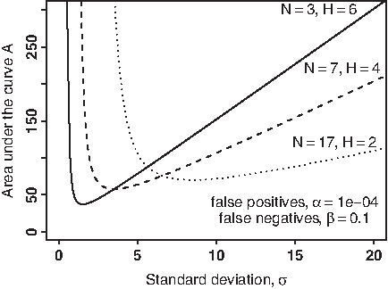
For a peptide signal to be detected, the corresponding Signal-to-Noise ratio must exceed the threshold F. Conversely, F expresses how well the detector is suited to the shape. Detection is easiest when F is minimal, i.e. when σ = N/2. However, the converse is not true, and given σ, the detector with parameter N/2 may not be optimal. For example, on Figure 2, the detector (H = 4, N = 7) performs best on elution profiles with σ = 3.5. As the dotted line is lower, there exists a different set of parameters that can detect lower-intensity signals.

FIG. 2.

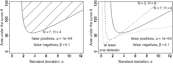
Limit of detection of the M-N rule. The shading lines indicate the set of shapes (A, σ) that a given detector can recall with probability greater than 90% based on Equations (3) and (4).

F does not depend on the noise distribution, but only on the Gaussian shape of the signals. As a consequence, a given detector is suited to a range of shapes that is roughly independent of noise distribution. More precisely, the two quantiles of the noise distribution \documentclass{aastex}\usepackage{amsbsy}\usepackage{amsfonts}\usepackage{amssymb}\usepackage{bm}\usepackage{mathrsfs}\usepackage{pifont}\usepackage{stmaryrd}\usepackage{textcomp}\usepackage{portland, xspace}\usepackage{amsmath, amsxtra}\pagestyle{empty}\DeclareMathSizes{10}{9}{7}{6}\begin{document} $$q_{{\cal N}, 1 - \alpha^{1 / N}}$$ \end{document} and \documentclass{aastex}\usepackage{amsbsy}\usepackage{amsfonts}\usepackage{amssymb}\usepackage{bm}\usepackage{mathrsfs}\usepackage{pifont}\usepackage{stmaryrd}\usepackage{textcomp}\usepackage{portland, xspace}\usepackage{amsmath, amsxtra}\pagestyle{empty}\DeclareMathSizes{10}{9}{7}{6}\begin{document} $$q_{{\cal N}, 1 - (1 - \beta)^{1 / N}}$$ \end{document} affect the lower limit of detection, but not the adequacy between σ and N. In particular, the simulations presented on Figure 2 are expected to accurately reflect the real detection range in LC/MS images (For a comparison with Gaussian Noise, see Figure 12 in Supplementary Material, available at www.liebertonline.com/cmb.)

To draw Figure 2, we assume that \documentclass{aastex}\usepackage{amsbsy}\usepackage{amsfonts}\usepackage{amssymb}\usepackage{bm}\usepackage{mathrsfs}\usepackage{pifont}\usepackage{stmaryrd}\usepackage{textcomp}\usepackage{portland, xspace}\usepackage{amsmath, amsxtra}\pagestyle{empty}\DeclareMathSizes{10}{9}{7}{6}\begin{document} $${\cal N}$$ \end{document} is a Poisson noise process with mean 3; this is consistent with the experimental dataset used in Section 3 which contains integer intensity values. We selected N = 7 and α = 10⁻⁴. Equation (3) leads to H = 4. We set the desired false-negative rate to β = 10% that is to say the level of confidence is 1 − β = 90%. In Figure 2, the left panel shows the set of shape parameters (A, σ) that the detector (H = 4, N = 7) can recall with probability over 90%. The right panel allows the comparison of the detectors (H = 4, N = 7) in solid line, (H = 6, N = 3) in dashed line and also the union of the sets for all choices of H and N in dotted line. The latter set thus delineates the fundamental limits of the M-N rule with regard to Gaussian signals.

We observe that no single detector is universal because it is not suited to arbitrarily small values of σ or large values of σ. This motivates the use of several detectors with varying values of N to increase coverage. However, the statistical analysis of combining the sets of detections obtained by different algorithms is again a multiple testing problem and is outside the scope of the present article.

Instead of using Poisson noise as the distribution of \documentclass{aastex}\usepackage{amsbsy}\usepackage{amsfonts}\usepackage{amssymb}\usepackage{bm}\usepackage{mathrsfs}\usepackage{pifont}\usepackage{stmaryrd}\usepackage{textcomp}\usepackage{portland, xspace}\usepackage{amsmath, amsxtra}\pagestyle{empty}\DeclareMathSizes{10}{9}{7}{6}\begin{document} $${\cal N} (t)$$ \end{document} , it is possible to estimate the background noise distribution in the LC/MS images and redraw the above diagram. This would be desirable to better adjust the parameters N and H. However, this is of no practical use because there are several background noise distributions in the LC/MS image. Background noise is usually more intense in the middle of the mass range and there is a periodic component that corresponds to background chemical impurities (proteolytic background, contaminants, [Keller et al., 2008]).

Conclusion. The range of detected low-intensity peptide signals varies significantly with the parameters of the detector. However, there remain shapes that cannot be detected by the M-N rule regardless of the parameters because these are below noise level. Even when the noise distribution is not known, Figure 2 can provide generic guidelines to select adequate values for H and N.

3. Results and Discussion

3.1. Description of the data set

We use the data set published in Klimek et al. (2008). A mix of 18 proteins was prepared and run on several mass spectrometry platforms including different types of instruments and replicates. The complete list of proteins in the standard sample is available, along with the experimental procedures used on each platform.

To evaluate the M-N rule feature detection algorithm, we focus on data acquired on a Q-TOF instrument. The illustrations in this article were generated using the file QT20060926_mix4_19.mzXML from mix4. This instrument has sufficient resolution to distinguish isotope patterns, and the data is acquired in profile mode rather than centroid mode. Note that this dataset contains intensity values that are all integers.

Centroiding is a signal processing algorithm that reduces the complexity and size of the data set. In doing so, it strongly affects MS signals and our binning procedure by shifting the position of data points. Moreover, it affects the background noise distribution by aggregating MS peaks; in particular, we can observe empty noise regions alongside high-intensity peaks in centroided data. This results in a unexpectedly high number of zeroes in the observed noise distribution. Centroiding is usually selected as a default option in manufacturer software and cannot be undone.

3.2. Feature detection

Preprocessing. The experimental data was loaded from the mzXML data file and subsampled into pixels of width one scan and height of 0.1 Da. This is similar to binning each mass spectrum with bin width of 0.1 Da. We chose to set the intensity of each pixel to the sum or integral of the intensities of the peaks belonging to the pixel. The background noise distribution in the resulting LC/MS image appears uniform only in subregions of the data set. We chose to crop the data set to a retention time range rather than apply a normalisation tool to avoid potential biases, and consider the cropped LC/MS image as normalized.

We chose a narrow mass bin width of 0.1 Da, because at that resolution we can observe a 1 Da periodicity in the noise distribution and take it into account in the estimate of the parameter H. The periodicity is related to the background noise being chemical noise (i.e., random fragments of molecules including peptides). At the same time, the QTOF is an instrument with mass precision on the order of 50 ppm and provides many values for summing. Summing has two effects. First, it is a rudimentary smoothing operation that reduces the noise standard deviation with respect to its intensity. Second, due to the Central Limit Theorem, the noise distribution after summing is closer to Gaussian, which reduces quantization effects in the considered dataset and improves the estimation of the noise quantiles.

Noise quantiles. For each m/z bin, we approximate the threshold \documentclass{aastex}\usepackage{amsbsy}\usepackage{amsfonts}\usepackage{amssymb}\usepackage{bm}\usepackage{mathrsfs}\usepackage{pifont}\usepackage{stmaryrd}\usepackage{textcomp}\usepackage{portland, xspace}\usepackage{amsmath, amsxtra}\pagestyle{empty}\DeclareMathSizes{10}{9}{7}{6}\begin{document} $$H = q_{{\cal N}, 1 - \alpha^{1 / N}}$$ \end{document} with the empirical quantile computed from all the pixels in the mass bin. This is consistent with the assumption that the noise is independent and identically distributed. The estimate is unbiased; it does not lead to values of H that are systematically too strict or too lenient. This procedure is quick and provides one threshold per line. For unnormalized data, we advise using neighboring pixels in the mass bin to estimate the noise quantile.

The empirical quantile provides an estimate of H that is unbiased when there are no peptide signals in the m/z bin, and conservative in the presence of peptides. This is because peptide signals can only increase the quantile \documentclass{aastex}\usepackage{amsbsy}\usepackage{amsfonts}\usepackage{amssymb}\usepackage{bm}\usepackage{mathrsfs}\usepackage{pifont}\usepackage{stmaryrd}\usepackage{textcomp}\usepackage{portland, xspace}\usepackage{amsmath, amsxtra}\pagestyle{empty}\DeclareMathSizes{10}{9}{7}{6}\begin{document} $$q_{{\cal N}, 1 - \alpha^{1 / N}}$$ \end{document} . The false-positive rate always complies with the user-defined parameter α, regardless of the presence of peptides, and uniformly in the LC/MS image.

Feature detection. In this context, a pamphlet is a horizontal series of N pixels that corresponds to the binned intensity values in consecutive scans. According to the definition of the M-N rule in Section 2.5, a pamphlet contains a peptide signal if all the pixel intensities are above the threshold H. In the figures, when a pamphlet is detected, all the pixels belonging to the pamphlet are displayed.

Image results. In Figure 3, we show an example of detection with α = 10⁻³, N = 7. We observe that the detector can recall low-abundance signals with low error rate. Note that it recalls isotope patterns without a priori knowledge. We also verify that the detected signals do not display the 1Da period behaviour of the background noise. This means that the false-positive rate is independent of the changes in noise distribution at different m/z values.

FIG. 3.

Detection results with N = 7 and \documentclass{aastex}\usepackage{amsbsy}\usepackage{amsfonts}\usepackage{amssymb}\usepackage{bm}\usepackage{mathrsfs}\usepackage{pifont}\usepackage{stmaryrd}\usepackage{textcomp}\usepackage{portland, xspace}\usepackage{amsmath, amsxtra}\pagestyle{empty}\DeclareMathSizes{10}{9}{7}{6}\begin{document} $$H = q_{{\cal N}, 1 - \alpha^{1 / N}}$$ \end{document} (Left) Raw image. (Right) Only the areas where a peptide is detected.

In Figure 4, we show that α effectively controls the false-positive rate by displaying the detection results for several values for α. The user can set the false-positive rate regardless of the noise level and the detector adapts automatically by adjusting the threshold H. With higher false-positive rate, the detector is able to recall lower-intensity signals, which are not significant under stricter constraints. The predicted number of false positives (0.657 when α = 0.001) per line roughly matches the observations.

FIG. 4.

Detection results with varying false-positive rate \documentclass{aastex}\usepackage{amsbsy}\usepackage{amsfonts}\usepackage{amssymb}\usepackage{bm}\usepackage{mathrsfs}\usepackage{pifont}\usepackage{stmaryrd}\usepackage{textcomp}\usepackage{portland, xspace}\usepackage{amsmath, amsxtra}\pagestyle{empty}\DeclareMathSizes{10}{9}{7}{6}\begin{document} $$\alpha \in (0.1, 0.01, 0.001, 0.0001)$$ \end{document} . The expected number of false positives per line in the images is 65.7, 6.57, 0.657, and 0.0657, respectively. Bonferroni correction at level 5% would require α = 2.54 × 10⁻⁷.

3.3. Adjusting performance to signal shape

As emphasized in Section 2.6, the detector's performance is dependent on the signal shape. In this section, we compare three choices of the detector parameter \documentclass{aastex}\usepackage{amsbsy}\usepackage{amsfonts}\usepackage{amssymb}\usepackage{bm}\usepackage{mathrsfs}\usepackage{pifont}\usepackage{stmaryrd}\usepackage{textcomp}\usepackage{portland, xspace}\usepackage{amsmath, amsxtra}\pagestyle{empty}\DeclareMathSizes{10}{9}{7}{6}\begin{document} $$N \in \{3, 7, 17 \}$$ \end{document} . We first display the theoretical range of the detectors in Figure 5.

FIG. 5.

Theoretical detection range.

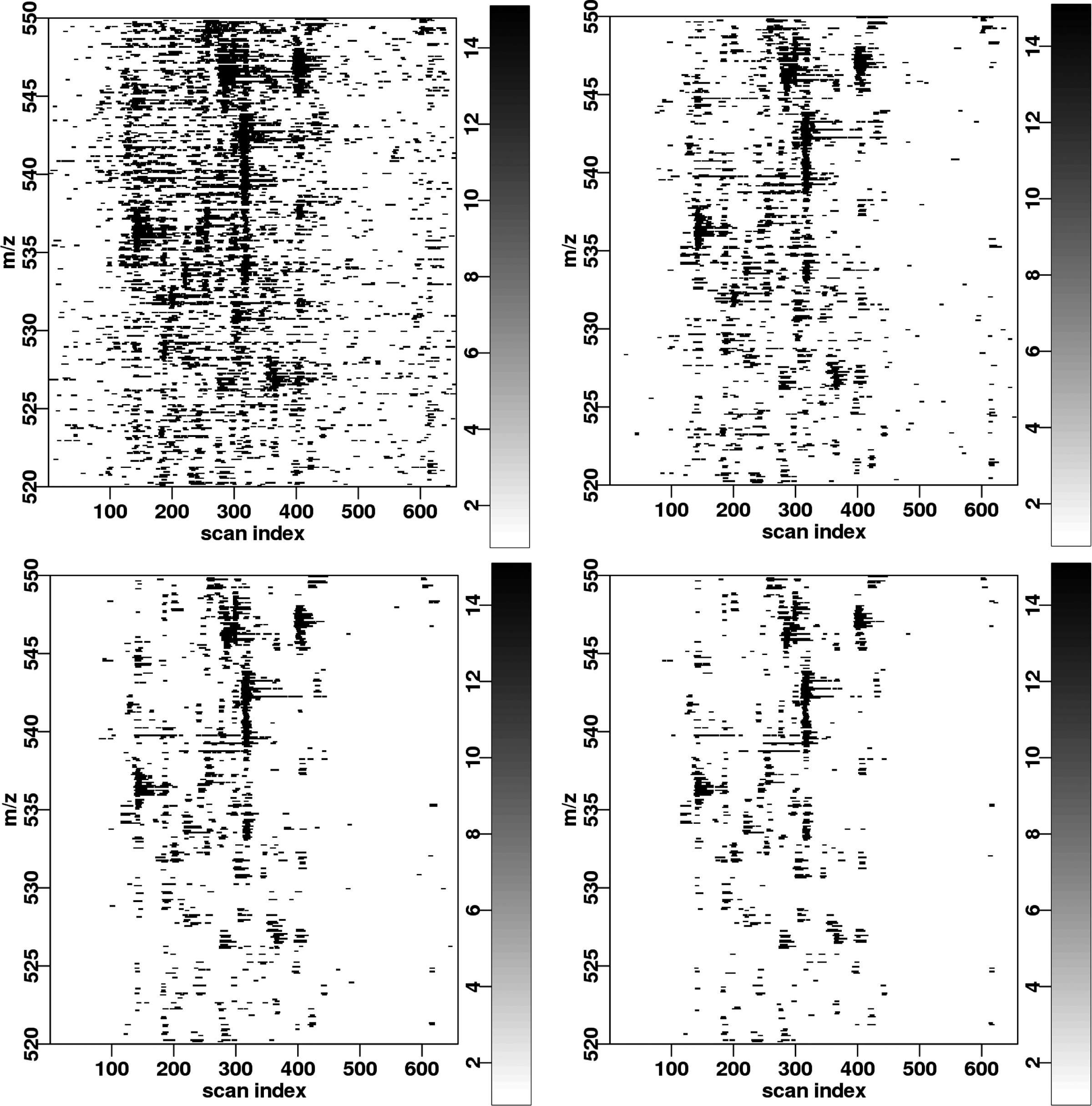
The selected detectors are suited to different ranges of σ. As a consequence, they do not detect the same peptide signals in the LC/MS image as shown in Figure 6. The (N = 3) detector is able to recall an isotopic pattern at (rt = 110, m/z = 707Da) which is missed by the (N = 17) detector. Conversely, the (N = 17) detector is able to recall signals of lower intensity at (rt = 50, m/z = 710Da) and especially the tails of the elution profiles. In this LC/MS image, the (N = 7) detector seems to be a good compromise.

FIG. 6.

Detection results with length parameter \documentclass{aastex}\usepackage{amsbsy}\usepackage{amsfonts}\usepackage{amssymb}\usepackage{bm}\usepackage{mathrsfs}\usepackage{pifont}\usepackage{stmaryrd}\usepackage{textcomp}\usepackage{portland, xspace}\usepackage{amsmath, amsxtra}\pagestyle{empty}\DeclareMathSizes{10}{9}{7}{6}\begin{document} $$N \in \{3, 7, 17 \}$$ \end{document} .

As indicated in Section 2.6, the M-N rule detector with parameters (N, H) is best suited for detecting Gaussian shapes of standard deviation σ = N/2. For other values of σ, the limit of detection is higher (increased area under the curve A). A reasonable heuristic for choosing N in practice thus consists in setting \documentclass{aastex}\usepackage{amsbsy}\usepackage{amsfonts}\usepackage{amssymb}\usepackage{bm}\usepackage{mathrsfs}\usepackage{pifont}\usepackage{stmaryrd}\usepackage{textcomp}\usepackage{portland, xspace}\usepackage{amsmath, amsxtra}\pagestyle{empty}\DeclareMathSizes{10}{9}{7}{6}\begin{document} $$N = 2 \hat{\sigma}$$ \end{document} where \documentclass{aastex}\usepackage{amsbsy}\usepackage{amsfonts}\usepackage{amssymb}\usepackage{bm}\usepackage{mathrsfs}\usepackage{pifont}\usepackage{stmaryrd}\usepackage{textcomp}\usepackage{portland, xspace}\usepackage{amsmath, amsxtra}\pagestyle{empty}\DeclareMathSizes{10}{9}{7}{6}\begin{document} $$\hat{\sigma}$$ \end{document} is the mean width of the observed elution profiles in the LC/MS image. Note that, in gradient elution, the liquid chromatography protocol can be adjusted so that the standard deviations of the elution profiles are roughly the same.

3.4. Comparison of the median and quantile M-N rule

In Radulovic et al. (2004), the authors propose using the Median M-N rule with the parameters (N = 3, H = 3*C), where C is 30% of the trimmed mean or the median. In this section, we discuss the advantages and the drawbacks of our proposed extension.

We compare the following two instantiations of the M-N rule:

• Quantile M-N rule with N = 3, \documentclass{aastex}\usepackage{amsbsy}\usepackage{amsfonts}\usepackage{amssymb}\usepackage{bm}\usepackage{mathrsfs}\usepackage{pifont}\usepackage{stmaryrd}\usepackage{textcomp}\usepackage{portland, xspace}\usepackage{amsmath, amsxtra}\pagestyle{empty}\DeclareMathSizes{10}{9}{7}{6}\begin{document} $$q_{{\cal N}, 1 - \alpha^{1 / N}}$$ \end{document} and α = 10⁻¹, and

• Median M-N rule with N = 3, H = 3 × C where C is the trimmed mean.

Both C and \documentclass{aastex}\usepackage{amsbsy}\usepackage{amsfonts}\usepackage{amssymb}\usepackage{bm}\usepackage{mathrsfs}\usepackage{pifont}\usepackage{stmaryrd}\usepackage{textcomp}\usepackage{portland, xspace}\usepackage{amsmath, amsxtra}\pagestyle{empty}\DeclareMathSizes{10}{9}{7}{6}\begin{document} $$q_{{\cal N}, 1 - \alpha^{1 / N}}$$ \end{document} are computed using the pixel intensities in the current m/z bin. In this dataset, the median cannot be used as proposed in Radulovic et al. (2004), because the noise has a low intensity and that intensity values are integers; in many mass bins, the median is equal to 0. As the level of trimming is unspecified in Radulovic et al. (2004), we chose to use symmetric 10% trimming.

In the original publication, the Median M-N rule is used after smoothing the intensities. This preprocessing step is not necessary for studying the properties of the M-N rule and is thus left out in the present article. Smoothing can be applied before both algorithms with the following caveat. Smoothing reduces the noise variance, but introduces correlation between adjacent pixel intensities. As the pixel intensities are no longer independent, the false-positive rate computation in Section 2.5 is not valid. Consequently, smoothing may introduce artifacts in the detections for both the median M-N rule and the quantile M-N rule.

As seen in Section 4, the choice H = M × C in the Median M-N rule is not generic. It provides a uniform false-positive rate when the background noise distribution is Gaussian with mean C and standard deviation C, in which case \documentclass{aastex}\usepackage{amsbsy}\usepackage{amsfonts}\usepackage{amssymb}\usepackage{bm}\usepackage{mathrsfs}\usepackage{pifont}\usepackage{stmaryrd}\usepackage{textcomp}\usepackage{portland, xspace}\usepackage{amsmath, amsxtra}\pagestyle{empty}\DeclareMathSizes{10}{9}{7}{6}\begin{document} $$3 \times C = q_{{\cal N}, 0.977}$$ \end{document} . In general, this is not the case, and we provide the following examples:

• In the case of baseline variations, the mean background noise intensity is affected but not its standard deviation. If the mean intensity increases, then the median M-N rule becomes too strict.

• The next paragraph discusses in detail the case where N(t) is a Poisson random variable.

• Figure 7 uses a real dataset.

FIG. 7.

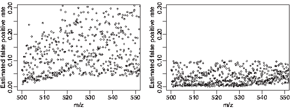
False-positive rate as a function of m/z for the Median M-N rule (left) and the Quantile M-N rule with α = 0.1 (right). In the extension, the false-positive rate is variable but obeys the upper bound.

Suppose that N(t) is a Poisson random variable with mean C between 5 and 10. We take N = 3 and α = 0.01. We set the remaining parameters for C = 7 which corresponds to a middle scenario between 5 and 10. The quantile M-N rule corresponds to (N = 3, H = 9). The median M-N rule corresponds to (N = 3, H = M × C) and we take M = 9/7 so that both have the same false-positive rate. In the regions of the LC/MS image where the noise intensity is lower, we have C = 5. The corresponding threshold for the quantile M-N rule is \documentclass{aastex}\usepackage{amsbsy}\usepackage{amsfonts}\usepackage{amssymb}\usepackage{bm}\usepackage{mathrsfs}\usepackage{pifont}\usepackage{stmaryrd}\usepackage{textcomp}\usepackage{portland, xspace}\usepackage{amsmath, amsxtra}\pagestyle{empty}\DeclareMathSizes{10}{9}{7}{6}\begin{document} $$H = q_{{\cal N}, 1 - \alpha^{1 / N}} = 7$$ \end{document} whereas the median M-N rule uses H = M × C = 6.43. Consequently, the median M-N rule is more lenient than the quantile M-N rule, and will lead to more false positives. In regions of high noise intensity, we have C = 10. The corresponding threshold for the quantile M-N rule is \documentclass{aastex}\usepackage{amsbsy}\usepackage{amsfonts}\usepackage{amssymb}\usepackage{bm}\usepackage{mathrsfs}\usepackage{pifont}\usepackage{stmaryrd}\usepackage{textcomp}\usepackage{portland, xspace}\usepackage{amsmath, amsxtra}\pagestyle{empty}\DeclareMathSizes{10}{9}{7}{6}\begin{document} $$H = q_{{\cal N}, 1 - \alpha^{1 / N}} = 12$$ \end{document} , whereas the median M-N rule uses H = M × C = 12.86. Consequently, the median M-N rule is too strict and will lead to false negatives. This example shows that the false-positive rate of the median M-N rule is not controlled in general. Moreover, the parameter M cannot be set such that the false-positive rate of the median M-N rule obeys a user-defined bound in both low noise intensity regions and high intensity regions. In this example, we have used the mean of the noise for C to simplify the computations; the same conclusions can be obtained when using the median or the trimmed mean.

On a real data set, we can illustrate the situation by deriving a theoretical value for the false-positive rate based on the local threshold used by each algorithm. For each algorithm, we compute the threshold H(m) in each mass bin, and use Equation (3) to obtain the predicted false-positive rate. In Figure 7, we observe that the computed false-positive rate for the Median M-N rule is very high and very variable as a function of m/z. On the other hand, the false-positive rate of the Quantile M-N rule obeys the selected bound α. The variations of the false-positive rate are due to quantisation in TOF data.

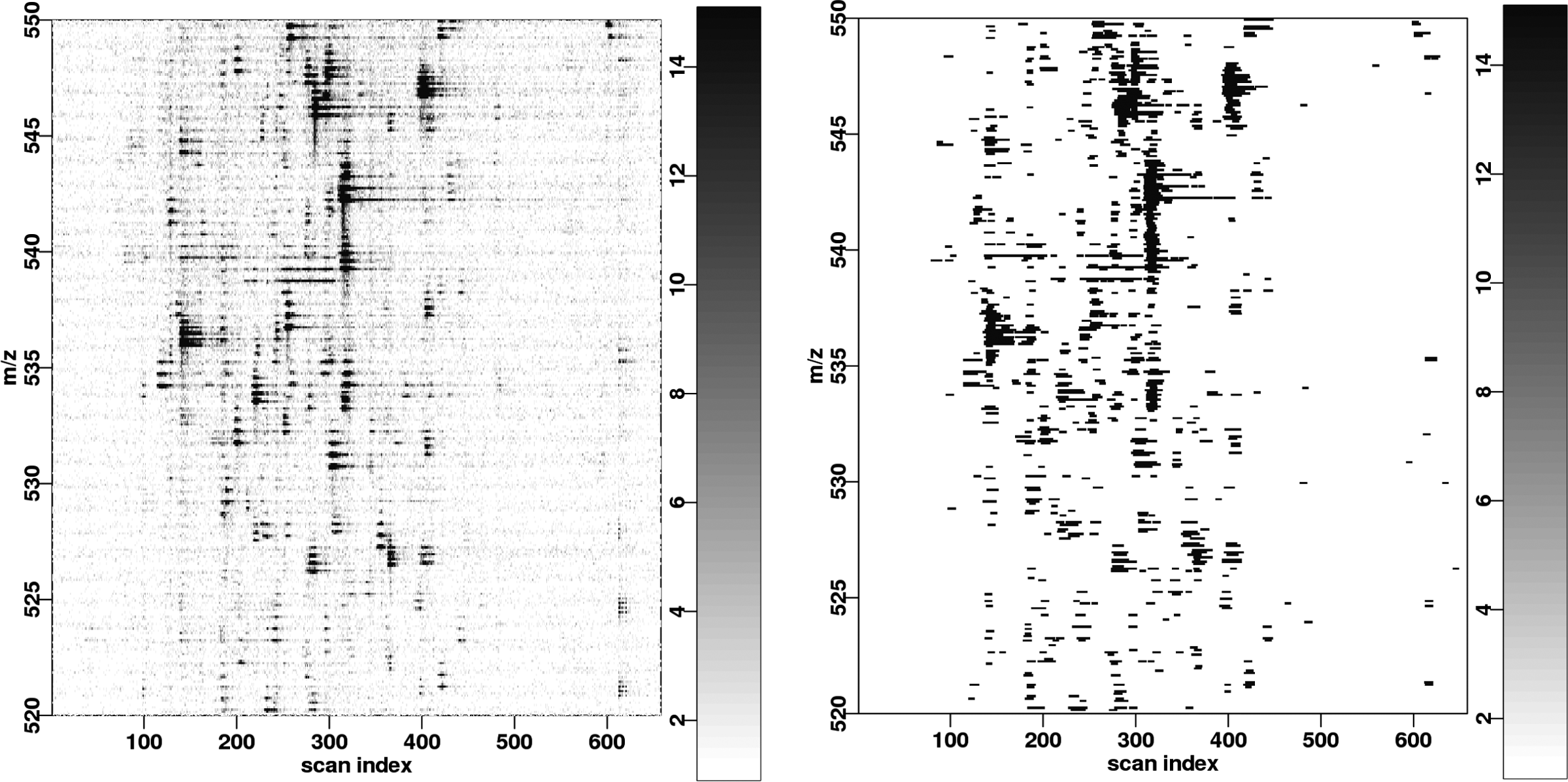
In Figure 8, we show the detection results obtained by the two algorithms on the same LC/MS image. In particular, we observe a periodic pattern with the original M-N rule that corresponds to the periodic behavior of the noise. This shows that the variations in noise intensity are not properly taken into account in the median M-N rule. A periodic pattern is not discernible in the results of the quantile M-N rule. In both cases, the high-intensity signals are adequately detected.

FIG. 8.

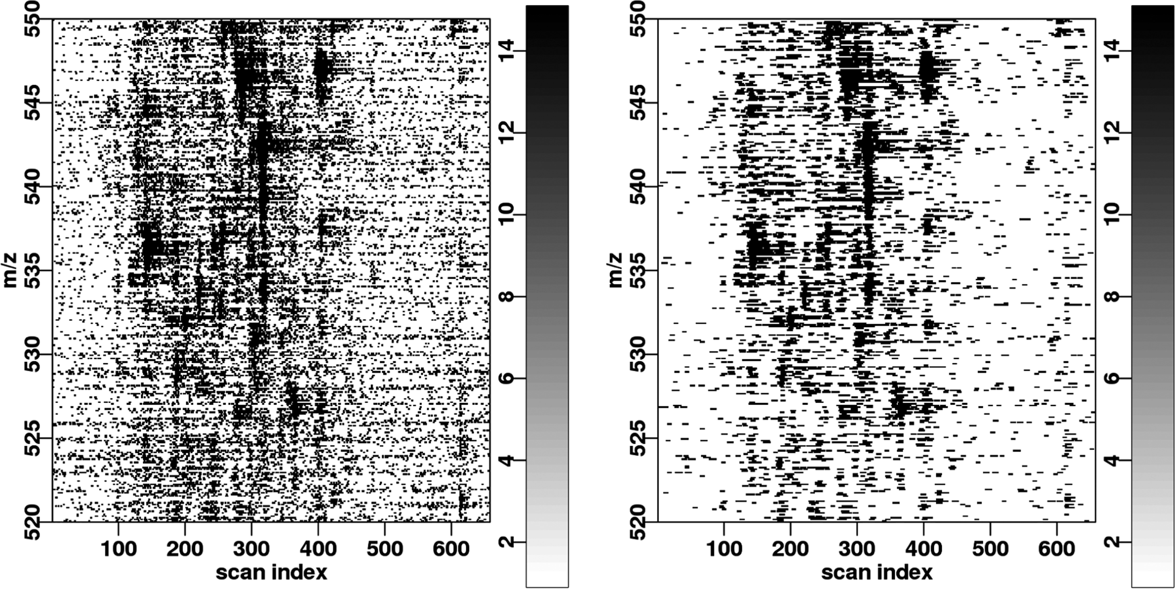
Detection with the Median M-N rule with parameters (N = 3, M = 3) and the Quantile M-N rule with parameters \documentclass{aastex}\usepackage{amsbsy}\usepackage{amsfonts}\usepackage{amssymb}\usepackage{bm}\usepackage{mathrsfs}\usepackage{pifont}\usepackage{stmaryrd}\usepackage{textcomp}\usepackage{portland, xspace}\usepackage{amsmath, amsxtra}\pagestyle{empty}\DeclareMathSizes{10}{9}{7}{6}\begin{document} $$(N = 3, H = q_{{\cal N}, 1 - \alpha^{1 / N}})$$ \end{document} with α = 0.1.

3.5. Discussion

The feature detection algorithm presented in this paper is generic and can be applied in many contexts. While we use normalized data to facilitate estimation of the noise level and its quantiles, only the hypothesis that noise intensities are independent is compulsory for the bound on the false-positive rate in Equation (4). Likewise, it can be applied to centroided data, although we expect the centroiding to affect the estimation of the noise quantiles. It guarantees a uniform false-positive rate in the LC/MS image, but also between images.

In Section 3.2, we assume that, after cropping, the data is normalised and that the noise component \documentclass{aastex}\usepackage{amsbsy}\usepackage{amsfonts}\usepackage{amssymb}\usepackage{bm}\usepackage{mathrsfs}\usepackage{pifont}\usepackage{stmaryrd}\usepackage{textcomp}\usepackage{portland, xspace}\usepackage{amsmath, amsxtra}\pagestyle{empty}\DeclareMathSizes{10}{9}{7}{6}\begin{document} $${\cal N} (t)$$ \end{document} is identically distributed. In our experience, when the mass spectrometer is not overloaded—usually in the middle of the time range—there is no visible time effect in the noise distribution (See Figure 10 in Supplementary Material, available at www.liebertonline.com/cmb.) However, at the beginning of the experiment, there may be very intense mass spectra that correspond to peptides that are not retained by the column chemistry, and are washed away. These will bias noise estimation and result in unnecessarily strict values for H. Likewise, when individual mass spectra are not normalised, the estimation of H may be incorrect. We chose to crop the dataset to avoid these two effects.

Independence is a critical assumption, which amounts to the absence of a memory effect between \documentclass{aastex}\usepackage{amsbsy}\usepackage{amsfonts}\usepackage{amssymb}\usepackage{bm}\usepackage{mathrsfs}\usepackage{pifont}\usepackage{stmaryrd}\usepackage{textcomp}\usepackage{portland, xspace}\usepackage{amsmath, amsxtra}\pagestyle{empty}\DeclareMathSizes{10}{9}{7}{6}\begin{document} $${\cal N} (t)$$ \end{document} and \documentclass{aastex}\usepackage{amsbsy}\usepackage{amsfonts}\usepackage{amssymb}\usepackage{bm}\usepackage{mathrsfs}\usepackage{pifont}\usepackage{stmaryrd}\usepackage{textcomp}\usepackage{portland, xspace}\usepackage{amsmath, amsxtra}\pagestyle{empty}\DeclareMathSizes{10}{9}{7}{6}\begin{document} $${\cal N} (t + 1)$$ \end{document} . Therefore, the M-N rule is best applied to raw data, without prior smoothing or baseline removal, as signal preprocessing may break the independence assumption. The baseline is mostly harmless and it is taken care of in the estimation of the local noise quantiles in the Quantile M-N rule. However, smoothing introduces correlation between adjacent pixel values and may lead to a higher false-positive rate than anticipated. (For more details, see Figure 11 in Supplementary Material, available at www.liebertonline.com/cmb.)

We analyzed the performance of the detector assuming a Gaussian model for the peak elution profile. Although this seems restrictive, it is useful and easy to interpret in terms of a Signal-to-Noise ratio. Violations of this assumption do not impact the computations in Section 2.5, so the bound on the false-positive rate is still assured, but the false-negative rate may be higher than expected. The detected features are not restricted to Gaussian signals and can address other (e.g., asymmetric) types of signal. (See Figure 9 in Supplementary Material, available at www.liebertonline.com/cmb.) The Signal-to-Noise ratio defined in Equation (5) remains valid under the condition that the elution profile width at height H matches that of a Gaussian function.

FIG. 9.

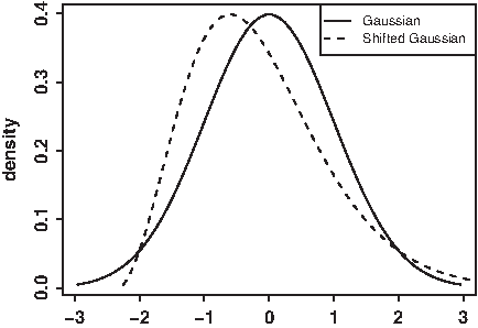
The computations for the specificity of the quantile M-N rule are still valid for non-Gaussian signals that have the same width at any height H. This includes asymmetric signals. The shifted signal in the example was obtained by replacing the x values with x + 0.15x² − 0.6.

Plots similar to Figure 2 may be used to compare different feature detection algorithms. However, fair comparison is only possible between algorithms with the same false-positive rate.

4. Conclusion

The Median M-N rule is a feature detection algorithm that can effectively recall low-intensity peptide signals in LC/MS images. In this article, we extend the original formulation and provide a precise account of the effect of the new parameters H and N on the detection results. N controls the standard deviation of the elution profiles that can be detected reliably, while H controls the selectivity of the algorithm. We provide guidelines for choosing N for a given LC/MS image and compute H from the local noise distribution. The resulting Quantile M-N rule is guaranteed to yield a false-positive rate bounded by a user-defined parameter α.

Feature detection with the M-N rule does not provide precise values for the signal retention time and m/z ratio. It does not tackle the deconvolution of overlapping features, nor does it take isotope patterns into account. When using the M-N rule, these tasks need to be handled by another algorithm with greater attention to individual pixel intensities in the pamphlet. However, the M-N rule can be used as a filtering step prior to accurate peak picking to provide a statistical control of the false-positive rate.

5. Appendix

Sensitivity of the M-N rule

In this section, we justify our approach to the computation of the sensitivity of the M-N rule. In a horizontal line, the recorded intensity is modeled as: \documentclass{aastex}\usepackage{amsbsy}\usepackage{amsfonts}\usepackage{amssymb}\usepackage{bm}\usepackage{mathrsfs}\usepackage{pifont}\usepackage{stmaryrd}\usepackage{textcomp}\usepackage{portland, xspace}\usepackage{amsmath, amsxtra}\pagestyle{empty}\DeclareMathSizes{10}{9}{7}{6}\begin{document} \begin{align*} {\cal I} (t) = {\cal N} (t) + A \frac {1} {\sqrt {2 \pi \sigma^2}} \exp {\left(- \frac {t^2} {2 \sigma^2} \right)} \end{align*} \end{document}

where \documentclass{aastex}\usepackage{amsbsy}\usepackage{amsfonts}\usepackage{amssymb}\usepackage{bm}\usepackage{mathrsfs}\usepackage{pifont}\usepackage{stmaryrd}\usepackage{textcomp}\usepackage{portland, xspace}\usepackage{amsmath, amsxtra}\pagestyle{empty}\DeclareMathSizes{10}{9}{7}{6}\begin{document} $${\cal N} (t)$$ \end{document} is the background noise and the signal is Gaussian, with area under the curve A, standard deviation σ and is centred in the pamphlet.

Given a false-positive rate α and the M-N rule parameters H and N, we compute the probability that a Gaussian signal with area under the curve A and standard deviation σ is detected by the M-N rule: \documentclass{aastex}\usepackage{amsbsy}\usepackage{amsfonts}\usepackage{amssymb}\usepackage{bm}\usepackage{mathrsfs}\usepackage{pifont}\usepackage{stmaryrd}\usepackage{textcomp}\usepackage{portland, xspace}\usepackage{amsmath, amsxtra}\pagestyle{empty}\DeclareMathSizes{10}{9}{7}{6}\begin{document} \begin{align*} {\mathbb P} [{\cal I}_i > H, \forall i \in \{ 1, \ldots, N \}] & = \prod_{i \in \{ 1, \ldots, N \}} {\mathbb P} [{\cal I}_i > H] \\ & = \prod_{i \in \{1, \ldots, N \}} {\mathbb P} \left[{\cal N} + \frac {A} {\sqrt {2 \pi \sigma^2}} \exp \left(- \frac {t_i^2} {2 \sigma^2} \right) > H \right] \\ & \geq \prod_{i \in \{1, \ldots, N \}} {\mathbb P} \left[{\cal N} + \frac {A} {\sqrt {2 \pi \sigma^2}} \exp \left(- \frac {N^2 / 4} {2 \sigma^2} \right) > H \right] \\ & = \left({\mathbb P} \left[{\cal N} + \frac {A} {\sqrt {2 \pi \sigma^2}} \exp \left(- \frac {N^2 / 4} {2 \sigma^2} \right) > H \right] \right)^N \end{align*} \end{document}

The lower bound is obtained because the Gaussian function Γ(t) is above the value Γ(N/2) in the range \documentclass{aastex}\usepackage{amsbsy}\usepackage{amsfonts}\usepackage{amssymb}\usepackage{bm}\usepackage{mathrsfs}\usepackage{pifont}\usepackage{stmaryrd}\usepackage{textcomp}\usepackage{portland, xspace}\usepackage{amsmath, amsxtra}\pagestyle{empty}\DeclareMathSizes{10}{9}{7}{6}\begin{document} $$t \in [- N / 2; N / 2]$$ \end{document} .

Given the false-negative rate β, we solve the following inequality: \documentclass{aastex}\usepackage{amsbsy}\usepackage{amsfonts}\usepackage{amssymb}\usepackage{bm}\usepackage{mathrsfs}\usepackage{pifont}\usepackage{stmaryrd}\usepackage{textcomp}\usepackage{portland, xspace}\usepackage{amsmath, amsxtra}\pagestyle{empty}\DeclareMathSizes{10}{9}{7}{6}\begin{document} \begin{align*} & \left({\mathbb P} \left[{\cal N} + \frac {A} {\sqrt {2 \pi \sigma^2}} \exp \left(- \frac {N^2 / 4} {2 \sigma^2} \right) > H \right] \right)^N \geq 1 - \beta \\ \Leftrightarrow \quad & {\mathbb P} \left[{\cal N} + \frac {A} {\sqrt {2 \pi \sigma^2}} \exp \left(- \frac {N^2 / 4} {2 \sigma^2} \right) > H \right] \geq (1 - \beta )^{1 / N} \\ \Leftrightarrow \quad & {\mathbb P} \left[{\cal N} + \frac {A} {\sqrt {2 \pi \sigma^2}} \exp \left(- \frac {N^2 / 4} {2 \sigma^2} \right) < H \right] \leq 1 - (1 - \beta )^{1 / N} \\ \Leftrightarrow \quad & H - \frac {A} {\sqrt {2 \pi \sigma^2}} \exp \left(- \frac {N^2 / 4} {2 \sigma^2} \right) \leq q_{{\cal N}, 1 - (1 - \beta)^{1 / N}} \end{align*} \end{document}

In conclusion we obtain: \documentclass{aastex}\usepackage{amsbsy}\usepackage{amsfonts}\usepackage{amssymb}\usepackage{bm}\usepackage{mathrsfs}\usepackage{pifont}\usepackage{stmaryrd}\usepackage{textcomp}\usepackage{portland, xspace}\usepackage{amsmath, amsxtra}\pagestyle{empty}\DeclareMathSizes{10}{9}{7}{6}\begin{document} \begin{align*} & H - q_{{\cal N}, 1 - (1 - \beta)^{1 / N}} \leq \frac {A} {\sqrt {2 \pi \sigma^2}} \exp \left(- \frac {N^2 / 4} {2 \sigma^2} \right) \\ & \Rightarrow \quad {\mathbb P} [{\cal I}_i > H, \forall i \in \{1, \ldots , N \}] \geq 1 - \beta . \end{align*} \end{document}

Footnotes

Acknowledgments

We thank the anonymous reviewer for very helpful comments. This work was supported by a Ph.D. thesis allowance from the French Ministry of Higher Education and Research.

Disclosure Statement

No competing financial interests exist.

References

Aebersold

, Mann

2003. Mass spectrometry-based proteomics. Nature, 422:198–207.

Anderle

, Roy

, Lin

et al. 2004. Quantifying reproducibility for differential proteomics: noise analysis for protein liquid chromatography-mass spectrometry of human serum. Bioinformatics, 20:3575–3582.

Andreev

V.P.

, Rejtar

, Chen

H.S.

et al. 2003. A universal denoising and peak picking algorithm for LC-MS based on matched filtration in the chromatographic time domain. Anal. Chem, 75:6314–6326.

Bantscheff

, Schirle

, Sweetman

et al. 2007. Quantitative mass spectrometry in proteomics: a critical review. Anal. Bioanal. Chem., 389:1017–1031.

Bellew

, Coram

, Fitzgibbon

et al. 2006. A suite of algorithms for the comprehensive analysis of complex protein mixtures using high-resolution LC-MS. Bioinformatics, 22:1902.

Coombes

K.R.

, Tsavachidis

, Morris

J.S.

et al. 2005. Improved peak detection and quantification of mass spectrometry data acquired from surface-enhanced laser desorption and ionization by denoising spectra with the undecimated discrete wavelet transform. Proteomics, 5:16.

Currie

L.A.

1999. Detection and quantification limits: origins and historical overview. Anal. Chim. Acta, 391:127–134.

Desolneux

, Moisan

, Morel

J.M.

2000. Meaningful alignments. Int. J. Comput. Vision, 40:7–23.

Desolneux

, Moisan

, Morel

J.M.

2001. Edge detection by Helmholtz principle. J. Math. Imaging Vision, 14:271–284.

10.

Domon

, Aebersold

2006. Mass spectrometry and protein analysis. Science, 312:212–217.

11.

, Kibbe

W.A.

, Lin

S.M.

2006. Improved peak detection in mass spectrum by incorporating continuous wavelet transform-based pattern matching. Bioinformatics, 22:2059.

12.

Eng

J.K.

, McCormack

A.L.

, Yates

J.R.

1994. An approach to correlate tandem mass spectral data of peptides with amino acid sequences in a protein database. J. Am. Soc. Mass Spectrom., 5:976–989.

13.

Felinger

1998. Data Analysis and Signal Processing in Chromatography. Elsevier Science Ltd.: New York.

14.

Fenyo

, Beavis

R.C.

2003. A method for assessing the statistical significance of mass spectrometry-based protein identifications using general scoring schemes. Anal. Chem, 75:768–774.

15.

Frank

A.M.

, Savitski

M.M.

, Nielsen

M.N.

et al. 2007. De novo peptide sequencing and identification with precision mass spectrometry. J. Proteome Res., 6:114.

16.

Gras

, Muller

, Gasteiger

et al. 1999. Improving protein identification from peptide mass fingerprinting through a parameterized multi-level scoring algorithm and an optimized peak detection. Electrophoresis, 20:18.

17.

Hastings

C.A.

, Norton

S.M.

, Roy

2002. New algorithms for processing and peak detection in liquid chromatography/mass spectrometry data. Rapid Commun. Mass Spectrom., 16:462–467.

18.

Hilario

, Kalousis

, Pellegrini

et al. 2006. Processing and classification of protein mass spectra. Mass Spectrom. Rev., 25:3.

19.

Howard

B.A.

, Wang

M.Z.

, Campa

M.J.

et al. 2003. Identification and validation of a potential lung cancer serum biomarker detected by matrix-assisted laser desorption/ionization-time of flight spectra analysis. Proteomics, 3:9.

20.

Jaitly

, Page-Belanger

, Faubert

et al. 2004. MSMS peak identification and its applications. ISMB/ECCB, 2004:1–3.

21.

Jeffries

2005. Algorithms for alignment of mass spectrometry proteomic data. Bioinformatics, 21:3066–3073.

22.

Jin

, Xue

, Zhang

et al. 2008. Prediction of retention times and peak shape parameters of unknown compounds in traditional Chinese medicine under gradient conditions by ultra performance liquid chromatography. Anal. Chim. Acta, 628:95–103.

23.

Kalousis

, Prados

, Rexhepaj

et al. 2005. Feature extraction from mass spectra for classification of pathological states. Lect. Notes Comput. Sci., 3721:536.

24.

Kast

, Gentzel

, Wilm

et al. 2003. Noise filtering techniques for electrospray quadrupole time of flight mass spectra. J. Am. Soc. Mass Spectrom., 14:766–776.

25.

Katajamaa

, Oresic

2005. Processing methods for differential analysis of LC/MS profile data. BMC Bioinform., 6:179.

26.

Keller

B.O.

, Sui

, Young

A.B.

et al. 2008. Interferences and contaminants encountered in modern mass spectrometry. Anal. Chim. Acta, 627:71–81.

27.

Kempka

, Sjodahl

, Bjork

et al. 2004. Improved method for peak picking in matrix-assisted laser desorption/ionization time-of-flight mass spectrometry. Rapid Commun. Mass Spectrom., 18:11.

28.

Kitteringham

N.R.

, Jenkins

R.E.

, Lane

C.S.

et al. Multiple reaction monitoring for quantitative biomarker analysis in proteomics and metabolomics. J. Chromatogr. B Anal. Technol. Biomed. Life Sci.

29.

Klimek

, Eddes

J.S.

, Hohmann

et al. 2008. The Standard Protein Mix Database: a diverse data set to assist in the production of improved peptide and protein identification software tools. J. Proteome Res, 7:96–103.

30.

Lange

, Gropl

, Reinert

et al. 2006. High-accuracy peak picking of proteomics data using wavelet techniques. Pac. Symp. Biocomput., 11:243–254.

31.

Leptos

K.C.

, Sarracino

D.A.

, Jaffe

J.D.

et al. 2006. MapQuant: open-source software for large-scale protein quantification. Proteomics, 6:1770–1782.

32.

2002. Comparison of the capability of peak functions in describing real chromatographic peaks. J. Chromatogr. A, 952:63–70.

33.

, Orlandi

, White

C.N.

et al. 2005. Independent validation of candidate breast cancer serum biomarkers identified by mass spectrometry. Clin. Chem., 51:2229–2235.

34.

Liu

, Krishnapuram

, Pratapa

et al. 2003. Identification of differentially expressed proteins using MALDI-TOF mass spectra. Signals Syst. Comput. 2003 Conf. Rec. 37th Asilomar Conf. 2.

35.

MacCoss. M.J., 2005. Computational analysis of shotgun proteomics data. Curr. Opin. Chem. Biol., 9:88–94.

36.

Malyarenko

D.I.

, Cooke

W.E.

, Adam

B.L.

et al. 2005. Enhancement of sensitivity and resolution of surface-enhanced laser desorption/ionization time-of-flight mass spectrometric records for serum peptides using time-series analysis techniques. Clin. Chem., 51:65–74.

37.

Mantini

, Petrucci

, Pieragostino

et al. 2007. LIMPIC: a computational method for the separation of protein MALDI-TOF-MS signals from noise. BMC Bioinform., 8:101.

38.

Morris

J.S.

, Coombes

K.R.

, Koomen

et al. 2005. Feature extraction and quantification for mass spectrometry in biomedical applications using the mean spectrum. Bioinformatics, 21:1764–1775.

39.

Naish

P.J.

, Hartwell

1998. Exponentially Modified Gaussian functions—A good model for chromatographic peaks in isocratic HPLC? Chromatographia, 26:285–296.

40.

Norbeck

A.D.

, Monroe

M.E.

, Adkins

J.N.

et al. 2005. The utility of accurate mass and LC elution time information in the analysis of complex proteomes. J. Am. Soc. Mass Spectrom, 16:1239–1249.

41.

Noy

, Fasulo

2007. Improved model-based, platform-independent feature extraction for mass spectrometry. Bioinformatics, 23:2528.

42.

Perkins

D.N.

, Pappin

D.J.C.

, Creasy

D.M.

et al. 1999. Probability-based protein identification by searching sequence databases using mass spectrometry data. Electrophoresis, 20:18.

43.

Piening

B.D.

, Wang

, Bangur

C.S.

et al. 2006. Quality control metrics for lc/ms feature detection tools demonstrated on Saccharomyces cerevisiae proteomic profiles. J. Proteome Res., 5:1527–1534.

44.

, Adam

, Thornquist

et al. 2003. Data reduction using a discrete wavelet transform in discriminant analysis of very high dimensionality data. Biometrics, 143–151.

45.

Radulovic

, Jelveh

, Ryu

et al. 2004. Informatics platform for global proteomic profiling and biomarker discovery using liquid chromatography-tandem mass spectrometry. Mol. Cell Proteomics, 3:984–997.

46.

Randolph

T.W.

, Yasui

2006. Multiscale processing of mass spectrometry data. Biometrics, 62:589–597.

47.

Rejtar

, Chen

, Andreev

et al. 2004. Increased identification of peptides by enhanced data processing of high-resolution MALDI TOF/TOF mass spectra prior to database searching. Anal. Chem, 76:6017–6028.

48.

Sadygov

R.G.

, Cociorva

, Yates

J.R.

III . 2004. Large-scale database searching using tandem mass spectra: looking up the answer in the back of the book. Nat. Methods, 1:195–202.

49.

Satten

G.A.

, Datta

, Moura

et al. 2004. Standardization and denoising algorithms for mass spectra to classify whole-organism bacterial specimens. Bioinformatics, 20:17.

50.

Schulz-Trieglaff

, Pfeifer

, Gröpl

et al. 2008. LC-MSsim—a simulation software for liquid chromatography mass spectrometry data. BMC Bioinform., 9:423.

51.

Shin

, Mutlu

, Koomen

J.M.

et al. 2007. Parametric power spectral density analysis of noise from instrumentation in Maldi TOF mass spectrometry. Cancer Inform., 3:317–328.

52.

Simpson

D.C.

, Smith

R.D.

2005. Combining capillary electrophoresis with mass spectrometry for applications in proteomics. Electrophoresis, 26.

53.

Smith

R.D.

, Anderson

G.A.

, Lipton

M.S.

et al. 2002. An accurate mass tag strategy for quantitative and high-throughput proteome measurements. Proteomics, 2:513–523.

54.

Snyder

L.R.

, Glajch

J.L.

, Kirkland

J.J.

1997. Practical HPLC Method Development. Wiley: New York.

55.

Strittmatter

E.F.

, Rodriguez

, Smith

R.D.

2003. High mass measurement accuracy determination for proteomics using multivariate regression fitting: application to electrospray ionization time-of-flight mass spectrometry. Anal. Chem, 75:460–468.

56.

Tautenhahn

, Bottcher

, Neumann

2008. Highly sensitive feature detection for high resolution LC/MS. BMC Bioinform., 9:504.

57.

Tibshirani

, Hastie

, Narasimhan

et al. 2004. Sample classification from protein mass spectrometry, by “peak probability contrasts.” Bioinformatics, 20:3034–3044.

58.

Vandenbogaert

, Li-Thiao-T

, Kaltenbach

H.M.

et al. 2008. Alignment of LC-MS images, with applications to biomarker discovery and protein identification. Proteomics, 8:650–672.

59.

Wallace

W.E.

, Kearsley

A.J.

, Guttman

C.M.

2004. An operator-independent approach to mass spectral peak identification and integration. Anal. Chem., 76:2446–2452.

60.

Wang

, Zhu

, Pradhan

et al. 2006. Feature extraction in the analysis of proteomic mass spectra. Proteomics, 6:7.

61.

Wiese

, Reidegeld

K.A.

, Meyer

H.E.

et al. 2007. Protein labeling by iTRAQ: a new tool for quantitative mass spectrometry in proteome research. Proteomics, 7:3.

62.

Williams

, Cornett

, Dawant

et al. 2005. An algorithm for baseline correction of MALDI mass spectra. Proc. 43rd Annu. Southeast Reg. Conf, 137–142.

63.

Yang

, He

, Yu

2009. Comparison of public peak detection algorithms for MALDI mass spectrometry data analysis. BMC Bioinform., 10:4.

64.

Yasui

, Pepe

, Thompson

M.L.

et al. 2003. A data-analytic strategy for protein biomarker discovery: profiling of high-dimensional proteomic data for cancer detection. Biostatistics, 4:449–463.

65.

, Wu

, Lin

et al. 2006. Detecting and aligning peaks in mass spectrometry data with applications to MALDI. Comput. Biol. Chem., 30:27–38.

66.

Zhu

, Yu

C.Y.

, Zhang

2003a. Tree-based disease classification using protein data. Proteomics, 3:9.

67.

Zhu

, Wang

, Ma

et al. 2003b. Detection of cancer-specific markers amid massive mass spectral data. Proc. Nat. Acad. Sci. USA, 100:14666–14671.

Supplementary Material

Please find the following supplemental material available below.

For Open Access articles published under a Creative Commons License, all supplemental material carries the same license as the article it is associated with.

For non-Open Access articles published, all supplemental material carries a non-exclusive license, and permission requests for re-use of supplemental material or any part of supplemental material shall be sent directly to the copyright owner as specified in the copyright notice associated with the article.

0.00 MB

0.17 MB