A Near-Linear Time Algorithm for Haplotype Determination on General Pedigrees

Abstract

An O(nmα(m)) time algorithm is given for inferring haplotypes from genotypes of non-recombinant pedigree data, where n is the number of members, m is the number of sites, and α(m) is the inverse of the Ackermann function. The algorithm works on both tree and general pedigree structures with cycles. Constraints between pairs of heterozygous sites are used to resolve unresolved sites for the pedigree, enabling the algorithm to avoid problems previously experienced for non-tree pedigrees.

1. Introduction

Haplotypes indicate which gene variations are on which chromosome copy, while genotypes indicate only which gene variations are present at each site of the genome. In diploid organisms such as humans, usually only genotypes are collected since the cells of these organisms carry two copies of each chromosome, and a biochemical method to extract single chromosomes directly is expensive (Gusfield, 2002). Therefore, a computational methodology to infer haplotypes from genotypes is required. Data from a multigenerational family pedigree or from a population group can be used to deduce the haplotypes for all group members. Haplotype inference is complicated by recombinant data, where complementary parts of both of a parent's haplotypes can be inherited as a single combined haplotype of a child. Also complicating the problem are pedigree structures that are not trees, where there are multiple inheritance paths between some family members.

The haplotyping problem has been studied extensively in the last few years, both for pedigree and population data. If recombinations are allowed, the problem of inferring haplotypes for pedigrees with the minimum number of recombinations is NP-hard (Li and Jiang, 2003b). For reconstructing haplotype configurations for pedigree data, Qian and Beckmann (2002) proposed a rule-based algorithm with a time complexity O(2^dn²m³), where d is the largest number of children in a family, n is the number of members and m is the number of sites. The main principle of their algorithm is that the best haplotype configuration for pedigree data is the one that minimizes the number of recombination events, the Minimum-Recombinant Haplotype Configuration (MRHC) problem. Li and Jiang (2003a,b) proposed an O(dmn) block-extension algorithm for the MRHC problem using a greedy heuristic to resolve adjacent sites. However, as discussed in Li and Jiang (2004), this algorithm did not always find the haplotypes that minimized the number of recombinations, and worked under some restrictions. In order to improve the performance and handle missing data, an integer linear programming (ILP) formulation (Li and Jiang, 2004) was proposed, in which a branch-and-bound algorithm was used to narrow the search space. In fact, with missing data, the haplotyping problem is NP-hard even if there is no recombinant event in the genomic data (Liu et al. 2005). While inheritance in practice normally allows recombination, analysis of populations is discovering haplotype blocks (Gabriel et al. 2002), series of consecutive sites that are not known to be recombined. These discoveries enable us to limit data to blocks without recombination, especially for the close relationships found in pedigrees.

Various results exist for non-recombinant pedigree data, though the fastest algorithm deals specifically with tree pedigrees and cannot handle multiple inheritance paths. Haplotypes can be inferred for tree pedigrees in linear time (Chan et al. 2006), by capturing parity constraints between members and using them to resolve genotype sites. An O(nmα(n)) algorithm (Li and Li, 2008) is also proposed for tree pedigrees, with extensions to more complex pedigrees and missing data. However, the complexity of this algorithm does not hold for cycle pedigrees or pedigrees with missing data. For general pedigrees, an O(m³n³) algorithm (Li and Jiang, 2003b) represents and solves pedigree constraints using linear equations over the cyclic group Z₂; this algorithm has also been improved to take O(mn² + n³ log ²n log log n) time (Xiao et al., 2007) by eliminating redundant equations in the system. Several deduction techniques have also been combined into the program HAPLORE (Zhang et al., 2005), including a haplotype deduction algorithm (Qian and Beckmann, 2002), an inconsistent haplotype elimination algorithm (O'Connell and Weeks, 1999), and a haplotype frequency estimation algorithm (Qin et al., 2002). Though quick in practice, HAPLORE is largely described as a set of logic rules, and its computational complexity is not concretely specified.

In this article, we present an O(nmα(m)) time algorithm for inferring haplotypes from genotypes of non-recombinant pedigree data, where α(m) is the extremely slowly growing inverse of the Ackermann function. Basic concepts and motivation are given in Section 2. Sections 3 –7 step through the stages of the algorithm, with preliminary processing in Sections 3 and 4, and more complex computation in Sections 5 –7. Section 8 reports experimental results for randomly generated general pedigrees, which verifies correctness on more than 10,000 pedigrees and uses 640 of them to analyze the efficiency and need for the stages of the algorithm. The implemented algorithm's performance is measured using a variety of different criteria. This testing confirms the necessity and the efficiency of the stages, and shows that the algorithm ran very quickly and handled a variety of different pedigrees.

2. Basic Concepts

A member is an individual. A set of members is called a family if it includes only two parents and their children; it is a parent-offspring trio (hereafter a trio) if only two parents and one child are considered. A set of families connected through known family relationships is a pedigree. A parent is an internal parent if it is a child of another family; it is an external parent otherwise.

In diploid organisms, a cell contains two copies of each chromosome. The description data of the two copies are called a genotype, while those of a single copy are called a haplotype. A specific location in a chromosome is called a site, and its state is called an allele. There are two main types of sites: microsatellites and single nucleotide polymorphisms. A microsatellite site has several different states, while a single nucleotide polymorphism (SNP) site has exactly two possible states, denoted by 0 and 1. Only SNPs are considered in this article, like other works on haplotype inference.

If the states at a specific site in two haplotypes are the same, then this site is a homozygous site (0-0 or 1-1); if they differ, it is heterozygous (0-1 or 1-0). Two haplotypes combine together to form one genotype. Each member u has two haplotypes, denoted by h1_u and h2_u, which are vectors of 0 and 1's of length m, where m is the number of sites. The genotype of u, g_u, is a vector of 0's, 1's, and 2's of length m, where g_u[i] = 0 means h1_u[i] = 0 = h2_u[i], g_u[i] = 1 means h1_u[i] = 1 = h2_u[i], and where g_u[i] = 2 means {h1_u[i],h2_u[i]} = {0, 1}. We say h1_u and h2_u are consistent with g_u. The complement haplotype of a haplotype h at a heterozygous site is denoted by \documentclass{aastex}\usepackage{amsbsy}\usepackage{amsfonts}\usepackage{amssymb}\usepackage{bm}\usepackage{mathrsfs}\usepackage{pifont}\usepackage{stmaryrd}\usepackage{textcomp}\usepackage{portland, xspace}\usepackage{amsmath, amsxtra}\pagestyle{empty}\DeclareMathSizes{10}{9}{7}{6}\begin{document}$${\bar h}$$\end{document} , where \documentclass{aastex}\usepackage{amsbsy}\usepackage{amsfonts}\usepackage{amssymb}\usepackage{bm}\usepackage{mathrsfs}\usepackage{pifont}\usepackage{stmaryrd}\usepackage{textcomp}\usepackage{portland, xspace}\usepackage{amsmath, amsxtra}\pagestyle{empty}\DeclareMathSizes{10}{9}{7}{6}\begin{document}$${\bar h} = 1 - h$$\end{document} , so \documentclass{aastex}\usepackage{amsbsy}\usepackage{amsfonts}\usepackage{amssymb}\usepackage{bm}\usepackage{mathrsfs}\usepackage{pifont}\usepackage{stmaryrd}\usepackage{textcomp}\usepackage{portland, xspace}\usepackage{amsmath, amsxtra}\pagestyle{empty}\DeclareMathSizes{10}{9}{7}{6}\begin{document}$${\bar 0} = 1$$\end{document} and \documentclass{aastex}\usepackage{amsbsy}\usepackage{amsfonts}\usepackage{amssymb}\usepackage{bm}\usepackage{mathrsfs}\usepackage{pifont}\usepackage{stmaryrd}\usepackage{textcomp}\usepackage{portland, xspace}\usepackage{amsmath, amsxtra}\pagestyle{empty}\DeclareMathSizes{10}{9}{7}{6}\begin{document}$${\bar 1} = 0$$\end{document} .

The problem in this article is to find the haplotypes h1_u and h2_u for all members u, given their genotypes g_u. When g_u[i] = 0 or 1, then h1_u[i] and h2_u[i] are known, but if g_u[i] = 2, we may not yet know the value of h1_u[i] and h2_u[i], in which case we give the value “?.” In this case, the site is unresolved.

In the absence of recombinant events, haplotypes of members in a pedigree follow the Mendelian law of inheritance, where the two haplotypes of a child are transferred from its parents, one haplotype from its father and the other from its mother. In this work, we address the problem of inferring haplotypes for pedigree members based on their genotype data and the relationships between members. Our problem can be formally defined as follows.

Pedigree Haplotype Inference (PHI). Given a pedigree consisting of n members, and given a genotype g_u of length m for each member u, find haplotypes h1_u and h2_u for each member such that:

vector h1_u and h2_u are consistent with g_u;

of an individual's two haplotypes, one is identical to one of the haplotypes of one parent, and the other is identical to one of the haplotypes of the other parent.

In the PHI problem, all genotype values are from the same set of sites. If there are multiple sets of haplotypes that are consistent with the data, then all of them are determined. Each set of haplotypes is called a haplotype configuration.

Chan et al. (2006) propose a linear time algorithm for inferring haplotypes from genotypes. This algorithm works well with tree pedigree structures, but it does not work with a pedigree structure that has cycles. The problem with this algorithm is that it captures parity constraints between members for each site and thus cannot maintain parity constraints along paths once a cycle exists. We overcome this problem by capturing parity constraints among sites within each member. Our algorithm works on both tree and general pedigree structures.

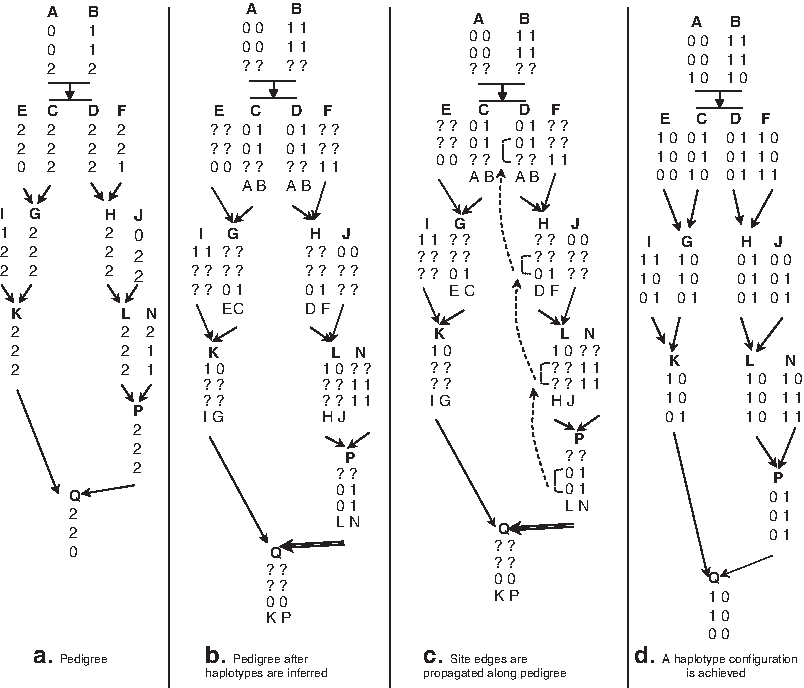
In this article, we use a running example (Fig. 1a) adapted from Chan et al. (2006) to illustrate the steps of our algorithm. We have added six more members to create a cycle in the pedigree that cannot be solved by the existing linear algorithm for tree pedigrees (Chan et al. 2006) due to the existence of multiple inheritance paths between members. In Figure 1a, the genotype of a member is displayed below the member's name. Each child in the pedigree has an arrow from each of its two parents.

FIG. 1.

Our pedigree after transformation phases.

The algorithm as implemented assumes every member has two parents or no parents. If a pedigree were to contain a member who has only one parent in the pedigree, we could add a second dummy external parent whose genotypes are all heterozygous, and thus generate any possible haplotype.

We use u and v to represent members, from 1 to n; and i, j, and r to represent sites, from 1 to m.

3. Initial Data Validation

The algorithm starts by validating the input genotypes along with the pedigree structure to ensure that all members satisfy the Mendelian law of inheritance, where the haplotypes of a child should come from its parents. In every family, a pattern is created from the genotypes of two parents u and v, and is used to validate against the genotypes of all children. The pattern p[i] for each site i (i = 1.m) is determined as follows:

g_u[i] = g_v[i] ≠ 2 → p[i] = g_u[i];

g_u[i] ≠ g_v[i],g_u[i] ≠ 2, and g_v[i] ≠ 2 → p[i] = 2;

g_u[i] = 0 or g_v[i] = 0 → p[i] ≠ 1 denoted by p[i] = ∼1;

g_u[i] = 1 or g_v[i] = 1 → p[i] ≠ 0 denoted by p[i] = ∼0;

otherwise p[i] = 3 (can be 0, 1 or 2).

These rules are listed in order of their priorities when creating a pattern. If the genotype of any child does not fit its pattern, the input data are invalid. For example, if a pattern is 1 2 3 ∼1 ∼0 and the genotypes of two children are 1 2 2 0 1 and 1 2 0 2 1, then the input data are potentially valid. However, if the genotype of a child is 1 2 2 1 1, then the input data are invalid in position 4, and the algorithm stops. Validating input data using patterns takes O(nm) time, since each child's genotype only needs to be validated against one pattern, and this requires comparisons in m sites.

In addition to validating the pedigree using patterns, every family is checked to ensure that there should not be any two sites i and j, which are heterozygous in two parents and both heterozygous or both homozygous in a child, but one homozygous and one heterozygous in another child; otherwise there is a family problem (Chan et al., 2006). Checking for a family problem can be done in O(nm) time (Chan et al., 2006). If there is no such violated family in the pedigree, we continue our algorithm; otherwise, the algorithm stops.

4. Haplotype Inferences

This section focuses on inferring haplotypes for each member and determining the origins for the inferred haplotypes.

4.1. Initial haplotype inferences

We infer haplotypes for each member by comparing genotypes of each trio in families, in a top-down traverse on the families of the pedigree. In each family, for every trio consisting of two parents u₁, u₂, and a child v, the haplotype pair 〈h1_v,h2_v〉 of v, where h1_v comes from u₁ and h2_v comes from u₂, is inferred as follows. For each site i:

if g_v[i] ≠ 2 then h1_v[i] = h2_v[i] = g_v[i]

if g_v[i] = 2 then

if \documentclass{aastex}\usepackage{amsbsy}\usepackage{amsfonts}\usepackage{amssymb}\usepackage{bm}\usepackage{mathrsfs}\usepackage{pifont}\usepackage{stmaryrd}\usepackage{textcomp}\usepackage{portland, xspace}\usepackage{amsmath, amsxtra}\pagestyle{empty}\DeclareMathSizes{10}{9}{7}{6}\begin{document}$$g_{u_{1}} [ i ] \neq 2$$\end{document} then \documentclass{aastex}\usepackage{amsbsy}\usepackage{amsfonts}\usepackage{amssymb}\usepackage{bm}\usepackage{mathrsfs}\usepackage{pifont}\usepackage{stmaryrd}\usepackage{textcomp}\usepackage{portland, xspace}\usepackage{amsmath, amsxtra}\pagestyle{empty}\DeclareMathSizes{10}{9}{7}{6}\begin{document}$$h1_{v} [ i ] = g_{u_{1}} [ i ] ; h2_{v} [ i ] = \overline{g_{u_{1}} [ i ] }$$\end{document}

The haplotype pair 〈h1_u1,h2_u1〉 of u₁ is inferred as follows. If the haplotypes of u₁ have not been previously inferred by any trio genotype comparison, let v be the child of u₁ that has the maximum number of resolved sites, h1_u1 is set to h1_v. For each site i:

if \documentclass{aastex}\usepackage{amsbsy}\usepackage{amsfonts}\usepackage{amssymb}\usepackage{bm}\usepackage{mathrsfs}\usepackage{pifont}\usepackage{stmaryrd}\usepackage{textcomp}\usepackage{portland, xspace}\usepackage{amsmath, amsxtra}\pagestyle{empty}\DeclareMathSizes{10}{9}{7}{6}\begin{document}$$h1_{u_{1}} [ i ] 1\neq?$$\end{document} then \documentclass{aastex}\usepackage{amsbsy}\usepackage{amsfonts}\usepackage{amssymb}\usepackage{bm}\usepackage{mathrsfs}\usepackage{pifont}\usepackage{stmaryrd}\usepackage{textcomp}\usepackage{portland, xspace}\usepackage{amsmath, amsxtra}\pagestyle{empty}\DeclareMathSizes{10}{9}{7}{6}\begin{document}$$h2_{u_{1}} [ i ] = \overline{h1_{u_{1}} [ i ] }$$\end{document} else \documentclass{aastex}\usepackage{amsbsy}\usepackage{amsfonts}\usepackage{amssymb}\usepackage{bm}\usepackage{mathrsfs}\usepackage{pifont}\usepackage{stmaryrd}\usepackage{textcomp}\usepackage{portland, xspace}\usepackage{amsmath, amsxtra}\pagestyle{empty}\DeclareMathSizes{10}{9}{7}{6}\begin{document}$$h2_{u_{1}} [ i ] = ?$$\end{document}

The haplotype pair 〈h1_u2,h2_u2〉 for u₂ is similarly resolved. Figure 1b shows partially inferred haplotypes for all members in the pedigree. The name of a member displayed below each inferred haplotype means the haplotype comes from that member. If all sites of members in the pedigree are resolved at the end of this phase, then one haplotype configuration is achieved, and the algorithm stops. Otherwise, we proceed to the next phase of our algorithm. The partial haplotype determination phase takes O(nm) computational steps.

4.2. Initial parental haplotype determination

One thing that is vital for any haplotype algorithm is to determine which haplotype of a parent is given to a child. In the following, u₁ and u₂ are the parents of child v, haplotype h1_v comes from u₁, and haplotype h2_v comes from u₂. We want to determine whether h1_v comes from \documentclass{aastex}\usepackage{amsbsy}\usepackage{amsfonts}\usepackage{amssymb}\usepackage{bm}\usepackage{mathrsfs}\usepackage{pifont}\usepackage{stmaryrd}\usepackage{textcomp}\usepackage{portland, xspace}\usepackage{amsmath, amsxtra}\pagestyle{empty}\DeclareMathSizes{10}{9}{7}{6}\begin{document}$$h1_{u_{1}}$$\end{document} or \documentclass{aastex}\usepackage{amsbsy}\usepackage{amsfonts}\usepackage{amssymb}\usepackage{bm}\usepackage{mathrsfs}\usepackage{pifont}\usepackage{stmaryrd}\usepackage{textcomp}\usepackage{portland, xspace}\usepackage{amsmath, amsxtra}\pagestyle{empty}\DeclareMathSizes{10}{9}{7}{6}\begin{document}$$h2_{u_{1}}$$\end{document} , and also whether h2_v comes from \documentclass{aastex}\usepackage{amsbsy}\usepackage{amsfonts}\usepackage{amssymb}\usepackage{bm}\usepackage{mathrsfs}\usepackage{pifont}\usepackage{stmaryrd}\usepackage{textcomp}\usepackage{portland, xspace}\usepackage{amsmath, amsxtra}\pagestyle{empty}\DeclareMathSizes{10}{9}{7}{6}\begin{document}$$h1_{u_{2}}$$\end{document} or \documentclass{aastex}\usepackage{amsbsy}\usepackage{amsfonts}\usepackage{amssymb}\usepackage{bm}\usepackage{mathrsfs}\usepackage{pifont}\usepackage{stmaryrd}\usepackage{textcomp}\usepackage{portland, xspace}\usepackage{amsmath, amsxtra}\pagestyle{empty}\DeclareMathSizes{10}{9}{7}{6}\begin{document}$$h2_{u_{2}}$$\end{document} .

Incompatible Haplotype. Let h1_v be the haplotype of a child v that comes from a parent u₁. If there is a resolved site i in h1_v and \documentclass{aastex}\usepackage{amsbsy}\usepackage{amsfonts}\usepackage{amssymb}\usepackage{bm}\usepackage{mathrsfs}\usepackage{pifont}\usepackage{stmaryrd}\usepackage{textcomp}\usepackage{portland, xspace}\usepackage{amsmath, amsxtra}\pagestyle{empty}\DeclareMathSizes{10}{9}{7}{6}\begin{document}$$h1_{u_{1}}$$\end{document} , where \documentclass{aastex}\usepackage{amsbsy}\usepackage{amsfonts}\usepackage{amssymb}\usepackage{bm}\usepackage{mathrsfs}\usepackage{pifont}\usepackage{stmaryrd}\usepackage{textcomp}\usepackage{portland, xspace}\usepackage{amsmath, amsxtra}\pagestyle{empty}\DeclareMathSizes{10}{9}{7}{6}\begin{document}$$h1_{v} [ i ] \neq h1_{u_{1}} [ i ]$$\end{document} , then \documentclass{aastex}\usepackage{amsbsy}\usepackage{amsfonts}\usepackage{amssymb}\usepackage{bm}\usepackage{mathrsfs}\usepackage{pifont}\usepackage{stmaryrd}\usepackage{textcomp}\usepackage{portland, xspace}\usepackage{amsmath, amsxtra}\pagestyle{empty}\DeclareMathSizes{10}{9}{7}{6}\begin{document}$$h1_{u_{1}}$$\end{document} and h1_v are incompatible. Otherwise, \documentclass{aastex}\usepackage{amsbsy}\usepackage{amsfonts}\usepackage{amssymb}\usepackage{bm}\usepackage{mathrsfs}\usepackage{pifont}\usepackage{stmaryrd}\usepackage{textcomp}\usepackage{portland, xspace}\usepackage{amsmath, amsxtra}\pagestyle{empty}\DeclareMathSizes{10}{9}{7}{6}\begin{document}$$h1_{u_{1}}$$\end{document} and h1_v are compatible.

Haplotype h1_v comes from \documentclass{aastex}\usepackage{amsbsy}\usepackage{amsfonts}\usepackage{amssymb}\usepackage{bm}\usepackage{mathrsfs}\usepackage{pifont}\usepackage{stmaryrd}\usepackage{textcomp}\usepackage{portland, xspace}\usepackage{amsmath, amsxtra}\pagestyle{empty}\DeclareMathSizes{10}{9}{7}{6}\begin{document}$$h1_{u_{1}}$$\end{document} iff \documentclass{aastex}\usepackage{amsbsy}\usepackage{amsfonts}\usepackage{amssymb}\usepackage{bm}\usepackage{mathrsfs}\usepackage{pifont}\usepackage{stmaryrd}\usepackage{textcomp}\usepackage{portland, xspace}\usepackage{amsmath, amsxtra}\pagestyle{empty}\DeclareMathSizes{10}{9}{7}{6}\begin{document}$$h1_{u_{1}}$$\end{document} and h1_v are compatible and \documentclass{aastex}\usepackage{amsbsy}\usepackage{amsfonts}\usepackage{amssymb}\usepackage{bm}\usepackage{mathrsfs}\usepackage{pifont}\usepackage{stmaryrd}\usepackage{textcomp}\usepackage{portland, xspace}\usepackage{amsmath, amsxtra}\pagestyle{empty}\DeclareMathSizes{10}{9}{7}{6}\begin{document}$$h2_{u_{1}}$$\end{document} and h1_v are incompatible. Haplotype h1_v comes from \documentclass{aastex}\usepackage{amsbsy}\usepackage{amsfonts}\usepackage{amssymb}\usepackage{bm}\usepackage{mathrsfs}\usepackage{pifont}\usepackage{stmaryrd}\usepackage{textcomp}\usepackage{portland, xspace}\usepackage{amsmath, amsxtra}\pagestyle{empty}\DeclareMathSizes{10}{9}{7}{6}\begin{document}$$h2_{u_{1}}$$\end{document} iff \documentclass{aastex}\usepackage{amsbsy}\usepackage{amsfonts}\usepackage{amssymb}\usepackage{bm}\usepackage{mathrsfs}\usepackage{pifont}\usepackage{stmaryrd}\usepackage{textcomp}\usepackage{portland, xspace}\usepackage{amsmath, amsxtra}\pagestyle{empty}\DeclareMathSizes{10}{9}{7}{6}\begin{document}$$h2_{u_{1}}$$\end{document} and h1_v are compatible and \documentclass{aastex}\usepackage{amsbsy}\usepackage{amsfonts}\usepackage{amssymb}\usepackage{bm}\usepackage{mathrsfs}\usepackage{pifont}\usepackage{stmaryrd}\usepackage{textcomp}\usepackage{portland, xspace}\usepackage{amsmath, amsxtra}\pagestyle{empty}\DeclareMathSizes{10}{9}{7}{6}\begin{document}$$h1_{u_{1}}$$\end{document} and h1_v are incompatible. If \documentclass{aastex}\usepackage{amsbsy}\usepackage{amsfonts}\usepackage{amssymb}\usepackage{bm}\usepackage{mathrsfs}\usepackage{pifont}\usepackage{stmaryrd}\usepackage{textcomp}\usepackage{portland, xspace}\usepackage{amsmath, amsxtra}\pagestyle{empty}\DeclareMathSizes{10}{9}{7}{6}\begin{document}$$g_{u_{1}} [ j ] \neq 2$$\end{document} at every site j, we can arbitrary set the origin of h1_v to either \documentclass{aastex}\usepackage{amsbsy}\usepackage{amsfonts}\usepackage{amssymb}\usepackage{bm}\usepackage{mathrsfs}\usepackage{pifont}\usepackage{stmaryrd}\usepackage{textcomp}\usepackage{portland, xspace}\usepackage{amsmath, amsxtra}\pagestyle{empty}\DeclareMathSizes{10}{9}{7}{6}\begin{document}$$h1_{u_{1}}$$\end{document} or \documentclass{aastex}\usepackage{amsbsy}\usepackage{amsfonts}\usepackage{amssymb}\usepackage{bm}\usepackage{mathrsfs}\usepackage{pifont}\usepackage{stmaryrd}\usepackage{textcomp}\usepackage{portland, xspace}\usepackage{amsmath, amsxtra}\pagestyle{empty}\DeclareMathSizes{10}{9}{7}{6}\begin{document}$$h2_{u_{1}}$$\end{document} .

If there is a haplotype of a child that comes from a parent but is incompatible with both haplotypes of that parent, the input data is invalid and the algorithm stops.

When the number of sites in each member is large, the possibility for determining the origins for all haplotypes in the pedigree using the above criteria is very high. However, for the illustration in the running example, we can determine the exact origin for only one haplotype in the pedigree. In Figure 1b, the parental haplotype of h2_Q is determined, denoted by a double line arrow coming from its parental haplotype h1_P. This initial determination of parental haplotypes for all haplotypes in a pedigree takes O(nm) time.

5. Graphs

There is more data that can be inferred about the haplotype data than is immediately obvious. First, let us introduce important properties of a pedigree.

Lemma 1

If u and v are a parent and a child in a family and there are two sites i and j heterozygous in both u and v, then the haplotype pairs at i and j in u and v are the same, {〈h1_u[i],h1_u[j]〉, 〈h2_u[i],h2_u[j]〉} = {〈h1_v[i],h1_v[j]〉, 〈h2_v[i],h2_v[j]〉}.

Proof. Because 〈h1_u[i],h1_u[j]〉 and 〈h2_u[i],h2_u[j]〉 are the alleles at i and j in the two haplotypes of u, and u is heterozygous at i and j, \documentclass{aastex}\usepackage{amsbsy}\usepackage{amsfonts}\usepackage{amssymb}\usepackage{bm}\usepackage{mathrsfs}\usepackage{pifont}\usepackage{stmaryrd}\usepackage{textcomp}\usepackage{portland, xspace}\usepackage{amsmath, amsxtra}\pagestyle{empty}\DeclareMathSizes{10}{9}{7}{6}\begin{document}$$h1_{u} [ i ] = \overline{h2_{u} [ i ] }$$\end{document} and \documentclass{aastex}\usepackage{amsbsy}\usepackage{amsfonts}\usepackage{amssymb}\usepackage{bm}\usepackage{mathrsfs}\usepackage{pifont}\usepackage{stmaryrd}\usepackage{textcomp}\usepackage{portland, xspace}\usepackage{amsmath, amsxtra}\pagestyle{empty}\DeclareMathSizes{10}{9}{7}{6}\begin{document}$$h1_{u} [ j ] = \overline{h2_{u} [ j ] }$$\end{document} .

If h1_u is transferred to, without loss of generality, h1_v, then 〈h1_v[i],h1_v[j]〉 is 〈h1_u[i],h1_u[j]〉. Because i and j are heterozygous in v, 〈h2_v[i],h2_v[j]〉 is \documentclass{aastex}\usepackage{amsbsy}\usepackage{amsfonts}\usepackage{amssymb}\usepackage{bm}\usepackage{mathrsfs}\usepackage{pifont}\usepackage{stmaryrd}\usepackage{textcomp}\usepackage{portland, xspace}\usepackage{amsmath, amsxtra}\pagestyle{empty}\DeclareMathSizes{10}{9}{7}{6}\begin{document}$$\langle \overline{h1_{v} [ i ] } , \overline{h1_{v} [ j ] } \rangle = \langle \overline{h1_{u} [ i ] } , \overline{h1_{u} [ j ] } \rangle = \langle h2_{u} [ i ] , h2_{u} [ j ] \rangle$$\end{document} . Thus, the haplotype pairs at i and j in u and v are the same.

If h2_u is transferred to, without loss of generality, h1_v, then 〈h1_v[i],h1_v[j]〉 is 〈h2_u[i],h2_u[j]〉. Because i and j are heterozygous in v, 〈h2_v[i],h2_v[j]〉 is \documentclass{aastex}\usepackage{amsbsy}\usepackage{amsfonts}\usepackage{amssymb}\usepackage{bm}\usepackage{mathrsfs}\usepackage{pifont}\usepackage{stmaryrd}\usepackage{textcomp}\usepackage{portland, xspace}\usepackage{amsmath, amsxtra}\pagestyle{empty}\DeclareMathSizes{10}{9}{7}{6}\begin{document}$$\langle \overline{h1_{v} [ i ] } , \overline{h1_{v} [ j ] } \rangle = \langle \overline{h2_{u} [ i ] } , \overline{h2_{u} [ j ] } \rangle = \langle h1_{u} [ i ] , h1_{u} [ j ] \rangle$$\end{document} . Thus, the haplotype pairs at i and j in u and v are the same even though the two haplotypes of v are exchanged. ▪

Corollary 1

If the genotypes of a parent and a child are identical, their haplotypes are the same.

Proof. Let 〈h1_u,h2_u〉 be the haplotype pair of a parent u. In every heterozygous site i, we have \documentclass{aastex}\usepackage{amsbsy}\usepackage{amsfonts}\usepackage{amssymb}\usepackage{bm}\usepackage{mathrsfs}\usepackage{pifont}\usepackage{stmaryrd}\usepackage{textcomp}\usepackage{portland, xspace}\usepackage{amsmath, amsxtra}\pagestyle{empty}\DeclareMathSizes{10}{9}{7}{6}\begin{document}$$h2_{u} [ i ] = \overline{h1_{u} [ i ] }$$\end{document} .

Without loss of generality, we consider that h1_u is transferred to h1_v of a child v. If genotypes of u and v are the same, then the haplotype pair of v at every heterozygous site i is \documentclass{aastex}\usepackage{amsbsy}\usepackage{amsfonts}\usepackage{amssymb}\usepackage{bm}\usepackage{mathrsfs}\usepackage{pifont}\usepackage{stmaryrd}\usepackage{textcomp}\usepackage{portland, xspace}\usepackage{amsmath, amsxtra}\pagestyle{empty}\DeclareMathSizes{10}{9}{7}{6}\begin{document}$$\langle h1_{v} [ i ] , h2_{v} [ i ] \rangle = \langle h1_{u} [ i ] , \overline{h1_{u} [ i ] } \rangle = \langle h1_{u} [ i ] , h2_{u} [ i ] \rangle$$\end{document} . Moreover, for every homozygous site j, if g_v[j] = g_u[j], then h1_u[j] = h2_u[j] = h1_v[j] = h2_v[j]. Therefore, if genotypes of u and v are the same, then 〈h1_v,h2_v〉 = 〈h1_u,h2_u〉. ▪

We extend the property in Lemma 1 to capture constraints of pairs of sites between members as follows.

Lemma 2

If u and v are two members and there are two sites i and j heterozygous in all members on a path from u to v, then the haplotype pairs at i and j in u and v are the same.

Corollary 2

If there is a path of members, where genotypes of all members on the path are identical, then haplotype pairs of the members are the same.

Since all members have the same genotypes, by Lemma 2 they have the same haplotype pairs.

To give an intuitive idea of our approach, consider Figure 1c where a green edge is inserted between two heterozygous sites 2 and 3 of P, reflecting that they have the same allele value (0 or 1). Since L is also heterozygous at sites 2 and 3, the haplotype pairs at these two sites of L are the same as those of P (Lemma 1). We transfer the green edge between sites 2 and 3 from P to L and similarly transfer this green edge to H and to D. Because the allele of site 3 of H is 0 and there is a green edge between sites 2 and 3, the allele of site 2 of H is 0. Similarly, the allele of site 3 of D is 0. Propagating these edges thus enables information from P to be used to resolve H and D without needing to resolve the intermediary L first. With these newly resolved sites, we can determine the original haplotypes for the haplotypes of D and H.

Other graphs are introduced to help in transferring data from one member to another.

5.1. Haplotype graph

We create a graph G_H = (V_H, E_H) of haplotypes. A node u in V_H is a haplotype, with two for each member. A black edge is created between two nodes if one node is the parental haplotype of the other node. Haplotypes connected by a path of black edges must be identical.

Data can be inserted into a haplotype when the other haplotype of its member is found. To facilitate these inferences, we insert blue edges into the haplotype graph joining the two haplotypes of each member of the pedigree. All the blue edges are inserted at initialization, while the black edges are determined later, if they can be determined.

5.2. Site graphs

The haplotype graph sometimes allows us to resolve all the heterozygous sites. However, in the experiments that we ran, about 26% required further processing, as indicated in Table 1 (see Section 8). In such a case, a site graph is constructed for each member. The nodes are member-site pairs (u,i), where the genomic data for a member u is heterozygous at site i. These are the sites that can determine black edges, because the data in the two haplotypes must be different. If two heterozygous sites are resolved and their alleles are the same, we insert a green edge between them. Otherwise, if their alleles are different, we insert a red edge between them.

Table 1.
Number of Times the Site Edge Propagation Is Used over 10 Cases

No. members

No. sites 10 20 40 80 160 320 640 1280

5 2 2 6 8 10 10 10 10

10 0 3 3 5 2 4 8 9

20 0 4 2 1 3 1 0 1

40 1 2 2 1 3 1 1 0

80 3 2 3 4 2 1 4 4

160 1 2 2 0 0 2 0 1

320 0 1 1 0 2 1 1 2

640 0 2 3 3 3 1 0 0

When an edge is inserted into a site graph, we check if they are in the same component, and if they are, we verify that the sites are resolved consistently. If they are in different components, then we replace the two components by their union, pointing the representative of the smaller component at the representative of the larger. The color of the edge joining the representatives is determined by the parity of the number of red edges on the paths joining the nodes to their representatives and the color of the inserted edge. We can do path compression on these forward edges, whenever we have to find out the component that a node is in, by pointing each node on this path at the component representative.

We cannot construct the whole site graph in linear time in general, but we do need to be able to resolve a site if it is connected by a path in the site graph to some other resolved site. To reduce the time complexity, we do not record all the edges of each site graph, but record only enough information so that the edge color can be determined quickly if we ever need it. To this end, we use the union-find data structure (Tarjan, 1975). We keep track of the connected components, and let one node represent each component. Each node points at another node which is closer to its representative, except that the representatives point at themselves. The color of the edges corresponding to these pointers are sufficient to work out the color of the edge between each node and its representative. The time complexity to build each site graph is O(mα(m)) (Tarjan, 1975).

One of the components of each site graph consists of the sites that have already been resolved. The other components are constructed from edge propagation, explained in the next section.

We also want to be able to find out all the elements in a given component in time proportional to the number of nodes in the component. To do this, we keep back pointers whenever an edge joins two formerly disconnected nodes. By following the back pointers, we can get to all the nodes in the connected component. The back pointers form a spanning tree of the component.

Figure 1c shows member P having two site components. The first component is site 1. The second component is sites 2 and 3, and there is a green edge between these two sites. The representative of the second component can be site 2.

6. Subroutines

There are four subroutines to insert and move data around these graphs:
Black edge insertion

Resolution of a heterozygous site of a member

Inserting an edge into a site graph

Edge propagation between site graphs

These operations are done in this order of priority. Operations 3 and 4 are only performed after site graphs are constructed, as operations 1 and 2 often completely solve the problem. Black edge insertion is performed as soon as a black edge is discovered. The next two operations, resolution and edge insertion into a site graph, both require more processing than just inserting data into the haplotypes. In both cases, we use queues to control the order of priority of operations, with the resolution taking precedence over the edge insertion. Edge propagation is done only after the queues are empty, when there is nothing else to do.

6.1. Black edge insertion

Immediately upon discovering that one haplotype is passed from a parent to a child, we insert a black edge joining these haplotypes into the haplotype graph, and resolve all sites that we can. To do this efficiently, we can find the sites that are newly resolved on each side of the new black edge. (Time complexity is O(m) per black edge: total O(nm).) The newly resolved sites are copied along all the black edges and inverted along blue edges, using depth first search. The time complexity is proportional to the amount of data to be updated, so is O(nm). If a discrepancy is found at this time because of a cycle in the pedigree graph, the algorithm stops.

Note that the initial parental haplotype determination (see Section 4.2) finds black edges.

6.2. Resolution of the site

When for whatever reason a haplotype site i is resolved in a member u, it is put into a queue for later processing. This later processing consists of:
a. Detecting and checking black edges:

For each member adjacent to u, if there already is a black edge between u and this member, and the member is already resolved at site i, we check to ensure that the two haplotypes joined by the black edge agree at site i. If there is a black edge and the other end is not resolved, then it can be resolved now, and the result added to the queue. If there is no black edge, and the site i is already resolved at the adjacent member, then a new black edge is determined and is inserted. If the neighbor is not resolved at site i, then there is nothing to do.

The total time complexity is O(nm) as each pair of adjacent members are considered at most m times from each end.

b. Resolving the other sites to which site i is connected in u's site graph:

This substep is done only if site graphs have been built. We follow the original back pointers from the current representative of the component and resolve every site found. We resolve a node the same as the representative if the path between these nodes contains an even number of red edges; otherwise, we resolve it the other way.

The time complexity of all such operations on a site graph is proportional to the number of edges of the spanning tree as each edge is looked at twice, once from each end.

c. Uniting resolved site components:

This substep is done only if site graphs have been built. The edge of u's site graph connecting the component of site i to the component of resolved sites is inserted between the components' representatives. It is colored green if these nodes are resolved the same and red if they are different.

6.3. Initial site graph construction

Before edge propagation starts, some preprocessing steps are done:
a. Setting up transitive links:

We traverse each edge of the pedigree graph; for each site such that the site is heterozygous in both members, we insert a transitive link between the site in each of the two site graphs at the equivalent site in the other site graph. This transitive link is colored green. This needs to be done only once for each (member, site) pair, so the combined time is O(nm).

b. Storing edges between resolved sites in site graphs:

In each site graph, as we insert an edge between two resolved sites i and j, we copy transitive links from one site to the other. Specifically, if i has a transitive link to site i′ in member v, but j does not have a transitive link to v, then we add a transitive link from j to i′ in v. Thus a site edge in a member has either 0 or 2 transitive links to each adjacent member. The color of the new transitive link is determined by the parity of the number of red edges on the path from j to i to i′. The total complexity of copying and coloring transitive links is O(nm) as each operation takes a constant time and the number of transitive links is bounded by the number of sites. We put all red and green edges in the component of resolved sites into the edge queue for later processing. Using the union-find data structure, only the spanning tree of site edges is formed and stored, so the time to store all edges is O(nmα(m)) (Tarjan, 1975).

c. Creating edges from homozygous sites:

If i and j are both homozygous sites in a member u, and both are heterozygous sites in a parental member v, then we create an edge between sites i and j in the site graph at v. It is colored green if g_u[i] = g_u[j] and colored red otherwise. This edge is put into the edge queue for later processing. The equivalent edges for children are already examined. Only a spanning tree of the heterozygous sites of the neighboring homozygous sites of u need to be created. The time to create these edges from all homozygous sites in all members to site graphs of their parental members is O(nm).

6.4. Inserting an edge into a site graph

Assume that we are to insert an edge between site i and site j in the site graph of a member u, and the color of the edge is known (red or green). From i we follow the forward pointers up the union-find tree, noting whether each node is resolved the same way or the opposite way with respect to i, until we come to the representative r of the component, which points at itself. Similarly we follow up from j to find the representative r′ for the other component.

If it turns out that r = r′, then the edge we were to insert is within one component of the site graph, and does not need to be added. We must check that the color to be inserted agrees. As we are using path compression we point every node that we passed on the way at their representative r = r′, and record the color of the edge from those nodes to r.

If r and r′ are different, then the edge joins two previously separate components. We assume that the component of r is at least as large as that of r′. We change the pointer at r′ to point at r, and add a backpointer at r′ onto the list of backpointers from r. We record the size of the component of r as the sum of the sizes of the two components. The color of these two pointers is green or red, depending on the parity of the number of red edges on the path from r to i to j to r′: green if even, red if odd. Again we point every node that we passed on the way at their representative r, and record the color of the edge from those nodes to r. The backpointers are not changed.

If one of the components involved is the resolved component, then all the sites of the other component can also be resolved. We can find the sites to be resolved by following the backpointers, and how to resolve them by the parity of the number of red edges on the path from them to r. The time complexity of this edge insertion is included in the analysis for edge propagation.

6.5. Edge propagation between site graphs

Assume that we have two sites i and j that are heterogenous in two adjacent members u and v. If the two sites are in the same component for member u but not in member v, then we can insert the edge between i and j in the site graph for v. The color of the new edge is the same as the color of the original, red or green. Propagating edges between site graphs is performed as follows.

We process the edges in the queue one at a time, to check if it can be propagated to the adjacent members. Let the dequeued edge join sites i and j in member u. Two operations are performed.

First, for child member v of u, if i is homozygous and j is heterozygous and unresolved in v, we resolve j using the color of the edge between i and j in the site graph of u.

Second, for member v adjacent to u, check if sites i and j have transitive links. If neither do, then nothing needs to be done. If both have transitive links, say i to i′ and j to j′, then we might be able to do an edge propagation, and, if we cannot, we still have to do a consistency check. Note that transitive links always point at sites which are heterozygous in the original site graph. Suppose i′ and j′ are in different components in the site graph for v, so that the edge from i′ to j′ can be propagated from u to v. As color must remain the same, we add a new edge in the site graph of v. Otherwise, if i′ and j′ are in the same component in the site graph for v, the edge does not need to be propagated, but we do a consistency check on the color of the existing edge and the color of the edge we would insert. If there is a color mismatch, the algorithm stops.

Note that a heterozygous site in a member can be a homozygous site in an adjacent member. Therefore, we cannot always transfer a site edge from a member to an identical location in another member like the situation in Figure 2a. There are some situations where an edge is transferred from a member to another member through an implied edge. Figure 2b shows such a situation, where sites 1, 2, 3, and 4 are all heterozygous in u while only sites 2 and 4 are heterozygous in v. Without the use of transitive links, any edge of u cannot be used directly to unite sites 2 and 4 in v. That is why transitive links are used, as they serve as anchors to transfer implied edges. When we unite sites 1, 2, 3 and 4 of u into one site component, we create transitive links trans(u₁,v₂) from site 1 of u to site 2 of v, and trans(u₃,v₂) from site 3 of u to site 2 of v. Therefore, edge ③ between sites 3 and 4 of u can be used to unite sites 2 and 4 in v. Here, the order of edges to be processed is not important and does not affect our algorithm due to using transitive links. We can process edges ①, ②, and ③ in any order, but we still can propagate the implied edge e₂₄ to v.

FIG. 2.
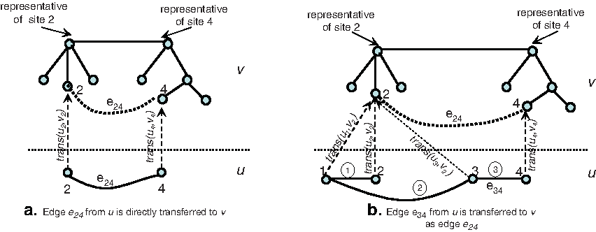
Transferring edges between members using transitive links.

As the number of edges in the site graphs is O(nm), the amount of work to be done is constant per operation except for finding the component representatives. Finding representatives is done using the union-find data structure, so the total work done is O(nmα(m)).

7. Completing the Haplotype Graph

It is possible that at some points none of the operations can be performed, yet there still are edges in the pedigree graph for which the haplotype inheritance is not yet determined. There are two cases: the end points are connected by a path in the haplotype graph, or they are not connected.

Suppose that the parent and child nodes of such an edge are connected by a path in the haplotype graph for which all the black edges have been determined. Then the edges and the path combine to form a cycle. In this case, we can determine which black edge must be chosen, depending on the following three sub-cases.

If there is a site that is heterozygous everywhere on the cycle, we determine the black edge to join endpoints of the missing edge such that the number of blue edges is even. If there is a site which is homozygous somewhere on the cycle but heterozygous at the parent node, then the cycle resolves this site at every member on the cycle, including at each endpoint of the missing edge. The black edge to be inserted is determined just by this single site. Otherwise, the parent node is homozygous at all sites so either black edge can be chosen as mentioned in Section 4.2.

After all cases of edges that form a cycle have been handled, every undetermined edge connects two different components of the haplotype graph. One cannot always choose any potential black edge, as shown in Figure 3. Each edge in the pedigree is labeled 0 if the left (right) haplotype of a parent is transferred to the left (right) haplotype of a child, and it is labeled 1 otherwise. If AB, AC, and DE are labeled 0, no other black edge is forced by the algorithm. Now choosing CE as either 0 or 1 causes a conflict on edge BD, since A, B, and C are left parents and D is a right Parent. However, choosing the black edges in the order AB, AC, BD leads to a solution (Fig. 3c).

Fig. 3.
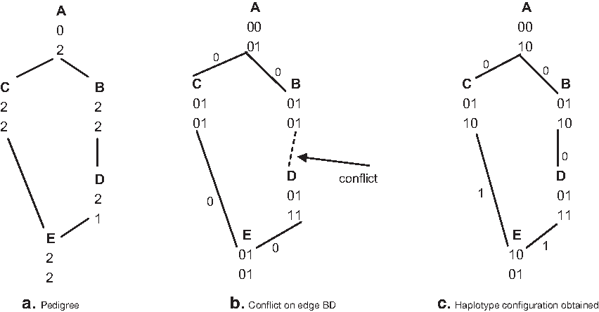
Completing haplotype graph.

Nevertheless one can in practice choose almost any potential black edge. Note that such a problem will not happen in tree pedigrees or pedigrees with one site heterozygous for all members as mentioned earlier in this section. It is unlikely to happen in practice as only one heterozygous and resolved site is required to distinguish which haplotype of a parent is transferred to a child. The problem is more likely to occur in cases with only two or three sites.

We conjecture that as long as the arbitrarily chosen black edges always occur in the same component of the haplotype graph, the algorithm will always find a solution. To satisfy this condition, the algorithm chooses the next black edge from among the edges joining this special component to other components.

8. Experimental Results

To verify the efficiency and the correctness of the algorithm, we have implemented our algorithm in C++ and tested it on more than 10,000 cases. The results for 640 cases were analyzed in detail. The remaining test cases were used to check the conjecture that the algorithm always works. The program and test data are available at www.cs.unb.ca/profs/pevans/research/phi.

Two parameters for a test case are specified, number n of members and number m of sites. The number of external parents is randomly generated ranging from 2 to \documentclass{aastex}\usepackage{amsbsy}\usepackage{amsfonts}\usepackage{amssymb}\usepackage{bm}\usepackage{mathrsfs}\usepackage{pifont}\usepackage{stmaryrd}\usepackage{textcomp}\usepackage{portland, xspace}\usepackage{amsmath, amsxtra}\pagestyle{empty}\DeclareMathSizes{10}{9}{7}{6}\begin{document}$$\left\lfloor \frac {n } {2 } \right\rfloor$$\end{document} members. A list of members is generated, initially containing only the external parents. We assign parents for each remaining member in the pedigree by randomly picking two members from the list of parents. If neither of the two parents has been assigned genders, their genders are assigned arbitrarily with opposite values. If only one of the parents has been assigned a gender, the gender of the other parent is assigned to be its opposite. Otherwise, if the genders of two parents are the same, two other parents are picked. The member with newly assigned parents is then added to the list of members and can become an internal parent. Any possible pedigree structure can be generated by this method, including highly complex pedigree structures with many cycles. We discard the resulting pedigree if it is not connected.

To generate genotypes for the pedigree, we first randomly generate haplotypes for external parents. Each child member randomly receives one haplotype from each parent based on the Mendelian law of inheritance. The genotype of a member is generated by combining its two generated haplotypes.

The following tables report experimental results from the first dataset, which contains 640 pedigrees. The values of n vary from 10 to 1280, and m from 5 to 640. For each (m, n) pair, 10 cases were generated. Seven features are reported in Tables 1 –7: number of times the site edge propagation step is used in the cases, average number of free choices, maximum number of free choices, average time to generate the first solution, maximum time to generate the first solution, average time to generate all solutions, maximum time to generate all solutions. A computer with a Dual-Core AMD 2.8GHz CPU and 16 GB of RAM was used.

Table 2.
Average Number of Free Choices

No. members

No. sites 10 20 40 80 160 320 640 1280

5 0.20 0.20 0.80 1.20 2.90 4.70 13.60 21.40

10 0.00 0.20 0.30 0.80 0.20 0.60 1.20 4.40

20 0.00 0.50 0.50 0.30 0.60 0.10 0.00 0.10

40 0.10 0.40 0.50 0.40 0.70 0.80 1.50 0.00

80 0.40 0.20 0.40 1.60 0.30 0.10 0.80 0.70

160 0.10 0.20 0.30 0.00 0.00 0.40 0.00 0.70

320 0.00 0.20 0.50 0.00 0.20 0.10 0.10 0.40

460 0.00 0.40 0.50 0.40 0.90 0.50 0.00 0.00

Table 3.
Maximum Number of Free Choices

No. members

No. sites 10 20 40 80 160 320 640 1280

5 1 1 2 2 7 8 45 33

10 0 1 1 3 1 2 3 25

20 0 2 3 3 3 1 0 1

40 1 2 4 4 4 8 15 0

80 2 1 2 9 2 1 3 4

160 1 1 2 0 0 2 0 7

320 0 2 5 0 1 1 1 3

640 0 2 3 2 6 5 0 0

Table 4.
Average Time (Seconds) to Generate the First Solution

No. members

No. sites 10 20 40 80 160 320 640 1280

5 0.11 0.14 0.42 0.75 2.03 4.04 10.56 23.39

10 0.04 0.14 0.24 0.60 0.75 1.73 4.07 10.78

20 0.04 0.21 0.30 0.40 0.94 1.45 2.51 5.44

40 0.07 0.19 0.30 0.42 1.02 1.57 3.36 4.94

80 0.18 0.14 0.31 0.97 0.93 1.40 4.84 9.85

160 0.06 0.16 0.32 0.31 0.63 2.18 2.53 7.56

320 0.04 0.19 0.38 0.31 1.68 2.44 5.01 14.62

640 0.04 0.46 1.07 2.47 4.92 4.06 2.64 5.48

Table 5.
Maximum Time (Seconds) to Generate the First Solution

No. members

No. sites 10 20 40 80 160 320 640 1280

5 0.42 0.48 0.96 1.18 3.07 6.63 24.83 30.29

10 0.05 0.44 0.48 1.30 1.15 2.83 5.01 22.73

20 0.05 0.61 1.08 1.35 2.11 2.93 3.00 10.84

40 0.40 0.67 1.39 1.57 2.72 3.94 11.00 6.26

80 0.71 0.42 0.91 3.48 2.34 4.00 8.61 18.63

160 0.33 0.52 0.98 0.37 0.79 6.35 3.46 29.78

320 0.05 1.27 2.44 0.38 6.32 12.18 25.58 52.66

640 0.05 2.00 3.61 7.83 16.65 29.87 3.25 7.34

Table 6.
Average Time (Seconds) to Generate First 256 Solutions

No. members

No. sites 10 20 40 80 160 320 640 1280

5 0.13 0.16 0.66 1.13 9.31 61.51 205.40 423.34

10 0.04 0.20 0.27 0.85 0.77 1.99 4.88 38.42

20 0.04 0.29 0.50 0.55 1.18 1.47 2.51 5.47

40 0.08 0.28 0.70 0.79 1.65 1.76 16.16 4.94

80 0.26 0.17 0.39 9.28 1.00 1.42 5.41 11.17

160 0.07 0.19 0.38 0.31 0.63 2.29 2.53 20.28

320 0.04 0.25 1.25 0.30 1.72 2.47 5.06 15.42

640 0.04 0.58 1.25 2.56 7.58 5.72 2.64 5.48

Table 7.
Maximum Time (Seconds) to Generate First 256 Solutions

No. members

No. sites 10 20 40 80 160 320 640 1280

5 0.52 0.57 2.35 2.58 52.79 282.42 456.41 1084.51

10 0.05 0.53 0.60 2.78 1.27 3.54 8.70 238.61

20 0.05 1.07 2.60 2.83 3.78 3.10 3.00 11.20

40 0.49 1.13 5.09 5.27 8.22 5.91 139.05 6.26

80 1.33 0.57 1.37 83.85 2.94 4.16 11.83 30.59

160 0.42 0.67 1.48 0.37 0.79 7.28 3.46 157.01

320 0.05 1.79 11.15 0.38 6.48 12.46 26.05 58.65

640 0.05 2.65 3.94 8.10 40.59 46.50 3.25 7.34

Since the number of solutions generated from a pedigree can be very large, the number of solutions is counted but only the first 256 solutions are generated. Moreover, whenever a choice of black edge is made, the current data structures are stored to generate all possible solutions later. However, storing data structures is time consuming and does affect the time to generate one solution. Therefore, another computation on the same dataset determines the time needed to generate one solution without storing data structures, as reported in Tables 8 and 9.

Table 8.
Average Time (Seconds) to Generate One Solution (No Storing Data Structures)

No. members

No. sites 10 20 40 80 160 320 640 1280

5 0.04 0.08 0.19 0.43 0.83 1.78 3.76 7.22

10 0.04 0.09 0.17 0.40 0.69 1.52 3.47 8.16

20 0.04 0.10 0.18 0.32 0.78 1.39 2.45 5.30

40 0.04 0.09 0.18 0.33 0.81 1.47 2.80 4.95

80 0.05 0.10 0.23 0.51 0.83 1.38 4.49 9.31

160 0.04 0.12 0.27 0.30 0.61 2.07 2.48 7.04

320 0.04 0.14 0.24 0.29 1.68 2.41 5.05 14.86

640 0.04 0.35 1.00 2.47 4.93 3.89 2.62 5.34

Table 9.
Maximum Time (Seconds) to Generate One Solution (No Storing Data Structures)

No. members

No. sites 10 20 40 80 160 320 640 1280

5 0.06 0.12 0.27 0.67 1.16 2.24 4.73 9.55

10 0.05 0.13 0.27 0.59 0.97 2.45 4.46 9.74

20 0.05 0.14 0.31 0.60 1.27 2.72 2.81 9.74

40 0.08 0.17 0.35 0.72 1.56 3.02 6.20 6.54

80 0.10 0.22 0.44 0.93 1.78 3.95 7.97 16.11

160 0.15 0.31 0.70 0.40 0.76 6.10 3.11 25.12

320 0.04 0.70 1.13 0.36 6.51 11.87 26.27 53.69

640 0.05 1.44 3.51 8.14 16.87 28.51 3.07 6.79

Table 1 shows the number of times the site edge propagation step is used to resolve new sites. The results show that the site edge propagation is used frequently, in 166 of the 640 cases. Site edge propagation is used more often when there are many members but few sites. The chance to determine the origins of haplotypes is higher when the number of sites is larger, which in turn can help to resolve more sites.

Similarly, the more sites a case has, the more chance that the origins of all haplotypes are determined just by the initial parental haplotype determination step. Therefore, the algorithm made many choices when the number of sites is small and the number of members is large, as shown in Tables 2 and 3. In the extreme case with 1280 members and 5 sites, there is an average of more than 21 choices, leading to more than two million solutions. When there were more than 20 sites, few cases had more than 1 choice.

Table 4 displays the average time, in seconds, to generate the first solution. It shows that the running time of the algorithm increased with the increase of the number of members, but appears to be independent of the number of sites. Actually, the running time of the program is not independent of the number of sites as shown in Tables 8 and 9. The time to generate one solution is much reduced when the number of sites increases, as shown in the last three columns of Table 4. Although smaller haplotypes are computed when the number of sites is small, the chance to completely determine the origins for all haplotypes is less. As a result, the program has to perform the site edge propagation step and spends time for storing data structures when free choices of black edges are made. When the number of sites is large, larger haplotypes are computed but are easier to distinguish, and fewer free choices are made. The program can solve any pedigree within a minute, as shown in Table 5.

Tables 6 and 7 display the average and the maximum times to generate multiple solutions of pedigrees. Since the number of solutions can be very large, 2³³, it is not possible to generate all of them. Instead, only the first 256 solutions will be generated. The program took only about 18 minutes to generate 256 solutions in the worst case.

The average and maximum times to generate multiple solutions depend on the number of free choices (Tables 2 and 3). In Tables 6 and 7, the pair (n = 80, m = 80) has an unexpectedly long time compared to other results in the same column. This is the result of a single unusual case with 9 free choices, taking 83.85 seconds to run.

Whenever a choice of black edge is made, the current data structures are stored to generate all possible solutions later. Storing data structures substantially increases the time to generate the first solution. Moreover, it is very difficult to conclude if the running time of the algorithm depends on the number of members and sites, especially when the number of choices is large. Aside from these issues, some users are only interested in finding one solution for a given pedigree. Therefore, another experiment is performed without storing the current data structures. The timing results appear in Tables 8 and 9.

According to these results, the running time of the program usually increases with the number of sites. This increase is more evident in Table 8 for the cases with 20, 40, and 160 members, where the number of times site edge propagation is used relatively the same (as shown in Table 1).

When n = 640 and m = 320, and n = 1280 and m = 230, the running times to generate one solution without storing data structures (Tables 8 and 9) are longer than storing data structures (Tables 4 and 5). The reason is that there are some cases among 10 datasets that have only one solution, which do not need to store data structures, and these cases unexpectedly ran faster in the previous testing as shown in Tables 4 and 5.

The program was also tested on a dataset containing more than 10,000 randomly generated pedigrees. The number of members increased from 10 to 640 and the number of sites from 5 to 635, with 10 values added for each increase. The experimentation always finds a solution, and thus supports the conjecture stated at the end of the previous section.

9. Conclusion

In this paper, we present an O(nmα(m)) time algorithm for inferring haplotypes from genotypes of non-recombinant pedigree data, where α(m) is the extremely slowly growing inverse of the Ackermann function. This nearly-linear time algorithm works on both tree and general pedigree structures, as confirmed by extensive experimentation, and comes from implementing the union-find data structure on graphs of related sites. Our result improves on the work of Xiao et al. (2007) by a factor of n and additionally handles cycle pedigree situations when compared to the work of Chan et al. (2006) and Li and Li (2008). Future work will determine how our algorithm can be extended to handle recombinant and missing data.

	No. members
5	2	2	6	8	10	10	10	10
10	0	3	3	5	2	4	8	9
20	0	4	2	1	3	1	0	1
40	1	2	2	1	3	1	1	0
80	3	2	3	4	2	1	4	4
160	1	2	2	0	0	2	0	1
320	0	1	1	0	2	1	1	2
640	0	2	3	3	3	1	0	0

	No. members
5	0.20	0.20	0.80	1.20	2.90	4.70	13.60	21.40
10	0.00	0.20	0.30	0.80	0.20	0.60	1.20	4.40
20	0.00	0.50	0.50	0.30	0.60	0.10	0.00	0.10
40	0.10	0.40	0.50	0.40	0.70	0.80	1.50	0.00
80	0.40	0.20	0.40	1.60	0.30	0.10	0.80	0.70
160	0.10	0.20	0.30	0.00	0.00	0.40	0.00	0.70
320	0.00	0.20	0.50	0.00	0.20	0.10	0.10	0.40
460	0.00	0.40	0.50	0.40	0.90	0.50	0.00	0.00

	No. members
5	1	1	2	2	7	8	45	33
10	0	1	1	3	1	2	3	25
20	0	2	3	3	3	1	0	1
40	1	2	4	4	4	8	15	0
80	2	1	2	9	2	1	3	4
160	1	1	2	0	0	2	0	7
320	0	2	5	0	1	1	1	3
640	0	2	3	2	6	5	0	0

	No. members
5	0.11	0.14	0.42	0.75	2.03	4.04	10.56	23.39
10	0.04	0.14	0.24	0.60	0.75	1.73	4.07	10.78
20	0.04	0.21	0.30	0.40	0.94	1.45	2.51	5.44
40	0.07	0.19	0.30	0.42	1.02	1.57	3.36	4.94
80	0.18	0.14	0.31	0.97	0.93	1.40	4.84	9.85
160	0.06	0.16	0.32	0.31	0.63	2.18	2.53	7.56
320	0.04	0.19	0.38	0.31	1.68	2.44	5.01	14.62
640	0.04	0.46	1.07	2.47	4.92	4.06	2.64	5.48

	No. members
5	0.42	0.48	0.96	1.18	3.07	6.63	24.83	30.29
10	0.05	0.44	0.48	1.30	1.15	2.83	5.01	22.73
20	0.05	0.61	1.08	1.35	2.11	2.93	3.00	10.84
40	0.40	0.67	1.39	1.57	2.72	3.94	11.00	6.26
80	0.71	0.42	0.91	3.48	2.34	4.00	8.61	18.63
160	0.33	0.52	0.98	0.37	0.79	6.35	3.46	29.78
320	0.05	1.27	2.44	0.38	6.32	12.18	25.58	52.66
640	0.05	2.00	3.61	7.83	16.65	29.87	3.25	7.34

	No. members
5	0.13	0.16	0.66	1.13	9.31	61.51	205.40	423.34
10	0.04	0.20	0.27	0.85	0.77	1.99	4.88	38.42
20	0.04	0.29	0.50	0.55	1.18	1.47	2.51	5.47
40	0.08	0.28	0.70	0.79	1.65	1.76	16.16	4.94
80	0.26	0.17	0.39	9.28	1.00	1.42	5.41	11.17
160	0.07	0.19	0.38	0.31	0.63	2.29	2.53	20.28
320	0.04	0.25	1.25	0.30	1.72	2.47	5.06	15.42
640	0.04	0.58	1.25	2.56	7.58	5.72	2.64	5.48

	No. members
5	0.52	0.57	2.35	2.58	52.79	282.42	456.41	1084.51
10	0.05	0.53	0.60	2.78	1.27	3.54	8.70	238.61
20	0.05	1.07	2.60	2.83	3.78	3.10	3.00	11.20
40	0.49	1.13	5.09	5.27	8.22	5.91	139.05	6.26
80	1.33	0.57	1.37	83.85	2.94	4.16	11.83	30.59
160	0.42	0.67	1.48	0.37	0.79	7.28	3.46	157.01
320	0.05	1.79	11.15	0.38	6.48	12.46	26.05	58.65
640	0.05	2.65	3.94	8.10	40.59	46.50	3.25	7.34

	No. members
5	0.04	0.08	0.19	0.43	0.83	1.78	3.76	7.22
10	0.04	0.09	0.17	0.40	0.69	1.52	3.47	8.16
20	0.04	0.10	0.18	0.32	0.78	1.39	2.45	5.30
40	0.04	0.09	0.18	0.33	0.81	1.47	2.80	4.95
80	0.05	0.10	0.23	0.51	0.83	1.38	4.49	9.31
160	0.04	0.12	0.27	0.30	0.61	2.07	2.48	7.04
320	0.04	0.14	0.24	0.29	1.68	2.41	5.05	14.86
640	0.04	0.35	1.00	2.47	4.93	3.89	2.62	5.34

	No. members
5	0.06	0.12	0.27	0.67	1.16	2.24	4.73	9.55
10	0.05	0.13	0.27	0.59	0.97	2.45	4.46	9.74
20	0.05	0.14	0.31	0.60	1.27	2.72	2.81	9.74
40	0.08	0.17	0.35	0.72	1.56	3.02	6.20	6.54
80	0.10	0.22	0.44	0.93	1.78	3.95	7.97	16.11
160	0.15	0.31	0.70	0.40	0.76	6.10	3.11	25.12
320	0.04	0.70	1.13	0.36	6.51	11.87	26.27	53.69
640	0.05	1.44	3.51	8.14	16.87	28.51	3.07	6.79

Footnotes

Disclosure Statement

No competing financial interests exist.

References

Chan

M.Y.

et al. 2006. Linear-time haplotype inference on pedigrees without recombinations. Lect. Notes comput. Sci., 4175:56–67.

Gabriel

et al. 2002. The structure of haplotype blocks in the human genome. Science, 296:2225–2229.

Gusfield

2004. An overview of combinatorial methods for haplotype inference. Lect. Notes comput. Sci., 2983:9–25.

, Jiang

2003a. Efficient inference of haplotypes from genotypes on a pedigree. J. Bioinform. Comput. Biol., 1:41–70.

, Jiang

2003b. Efficient rule-based haplotyping algorithms for pedigree data. Proc. RECOMB ’03, 197–206.

, Jiang

2004. An exact solution for finding minimum recombinant haplotype configurations on pedigrees with missing data by integer linear programming. Proc. RECOMB ’04, 20–29.

, Li

2008. Efficient haplotype inference from pedigrees with missing data using linear systems with disjoint-set data structures. Proc. 7th Annu. Int. Con. Comput. Syst. Bioinform., 297–308.

Liu

et al. 2005. Complexity and approximation of the minimum recombination haplotype configuration problem. Proc. ISAAC05, 370–379.

O'Connell

, Weeks

1999. An optimal algorithm for automatic genotype elimination. Am. J. Hum. Genet., 65:1733–1740.

10.

Qian

, Beckmann

2002. Minimum-recombinant haplotyping in pedigrees. Am. J. Hum. Genet., 70:1434–1445.

11.

Qin

Z.S.

et al. 2002. Partition-ligation-expectation-maximization algorithm for haplotype inference with single-nucleotide polymorphisms. Am. J. Hum. Genet., 71:1242–1247.

12.

Tarjan

R.E.

1975. Efficiency of a good but not linear set union algorithm. J. ACM, 22:215–225.

13.

Xiao

et al. 2007. Fast elimination of redundant linear equations and reconstruction of recombination-free mendelian inheritance on a pedigree. Proc. 18th Annu. ACM-SIAM Symp. Discrete Algorithms, 655–664.

14.

Zhang

et al. 2005. HAPLORE: a program for haplotype reconstruction in general pedigrees without recombination. Bioinformatics, 21:90–103.

	No. members
No. sites	10	20	40	80	160	320	640	1280
5	2	2	6	8	10	10	10	10
10	0	3	3	5	2	4	8	9
20	0	4	2	1	3	1	0	1
40	1	2	2	1	3	1	1	0
80	3	2	3	4	2	1	4	4
160	1	2	2	0	0	2	0	1
320	0	1	1	0	2	1	1	2
640	0	2	3	3	3	1	0	0