Explaining the Genetic Basis of Complex Quantitative Traits through Prediction Models

Abstract

The functional characterization of genes involved in many complex traits (phenotypes) of plants, animals, or humans can be studied from a computational point of view using different tools. We propose prediction—from the machine learning point of view—to search for the genetic basis of these traits. However, trying to predict an exact value of a phenotype can be too difficult to obtain a confident model, but predicting an approximation, in the form of an interval of values, can be easier. We shall see that trustable and useful models can be obtained from this relaxed formulation. These predictors may be built as extensions of conventional classifiers or regressors. Although the prediction performance in both cases are similar, we show that, from the classification field, it is straightforward to obtain a principled and scalable method to select a reduced set of features in these genetic learning tasks. We conclude by comparing the results so achieved in a real-world data set of barley plants with those obtained with state-of-the-art methods used in the biological literature.

1. Introduction

There are a number of complex traits or phenotypes of plants, animals, or humans that can be explained by their genetic descriptions or genotypes. One of the main purposes of modern genomics is to identify the genetic features (genes) responsible for the observed variability in these traits.

From a computational point of view, when we do not consider any pedigree information, genetic descriptions may be represented by vectors of feature values or genetic markers that are discrete items codifying the allelic composition, usually via SNP (single nucleotide polymorphism). On the other hand, a phenotype may be either a continuous or a discrete variable.

The type of relationship between genotypes and phenotypes, at its most basic level, is simply an association between a genetic marker and a phenotype that one can measure (Lynch and Walsh, 1998). However, most traits (phenotypes) are genetically complex; they are influenced by environmental causes and involve the joint action of many markers (Mauricio, 2001). This relationship has been recently formalized in terms of prediction power of phenotypes from genotypes (Bedo et al., 2008; Lee et al., 2008; Wray et al., 2007; Meuwissen et al., 2001).

Besides setting a formal framework, prediction has some interesting benefits (Lee et al., 2008). Thus, prediction is a natural way to assess the genetic risk of a disease in healthy individuals (Wray et al., 2007). Moreover, it has been reported (Meuwissen et al., 2001) that artificial selection on genetic values predicted from markers could substantially increase the rate of genetic gain in animals and plants.

In the references quoted above, the tools used for prediction are based on regression, even when the phenotype is represented by a binary variable. Regression is the obvious approach when the phenotype—i.e., the target value to be predicted—is continuous. However, frequently the genotype description is only partially available, and the environmental influence in the phenotype acts as a noise source, hindering the induction of a predictor. The consequence is that regressors may exhibit only modest performance scores, even when a strong relationship between genotype and phenotype exists.

To overcome the weaknesses of regression in this kind of learning tasks, we shall try to learn models to predict approximations to the phenotype values instead of exact values. To implement this idea, we relax the specifications of metric regression changing target points by intervals. Obviously, interval predictors are more reliable than metric regressors: the targets are broader.

There are two basic routes to make effective this approach. From the point of view of regression, to learn hypotheses whose predictions are intervals of a radius ε > 0, we may use the so-called ε-insensitive loss function, the loss used by regression support vector machines.

Additionally, we shall explore a second option, based on classification. We make a simple discretization of phenotype values into intervals of equal frequency; thus, predicting one of such intervals is a classification task. Moreover, we can take advantage of the ordering of those intervals; in fact, in this framework, learning the genetic basis of a phenotype is an ordinal regression task.

Moreover, the explanatory power of these classifiers can be additionally improved if we use set-valued classifiers. These classifiers return only one class (interval) when it is sufficiently sure, but in doubtful situations they may opt for predicting two or more classes (a wider interval). Set-valued classifiers have received different names in the literature. In Corani and Zaffalon (2008), the authors present an algorithm to learn set-valued classifiers called Nave Credal; it is an extension of the Nave Bayes classifier to imprecise probabilities.

In Alonso et al. (2008) and del Coz et al. (2009), these classifiers are called nondeterministic. We used them both for multiclass classification and for ordinal regression. The aim of the so-called nondeterministic hypothesis is to predict a set of classes (consecutive in ordinal regression) as small as possible, while still containing the true class. We proved that an optimal trade-off between size of predictions and successful classifications can be derived from the set of posterior probabilities for each entry of the input space. In other words, nondeterministic classifiers are built over a deterministic classifier (which always predicts one class) that provides posterior probabilities.

In this article, we present a slight modification of the algorithms of Alonso et al., (2008) and del Coz et al. (2009) to approach the genetic learning task introduced above. But the main novelty is that we establish that the 0/1 loss of a deterministic classifier is an upper bound of the nondeterministic loss of its nondeterministic counterpart. The consequence is that those tools specially devised to improve deterministic classifiers' performance can be used in nondeterministic learning tasks. More specifically, feature selection algorithms designed for deterministic classifiers can be used with nondeterministic learners to obtain a fully scalable method, suitable for dealing with large genetic data sets. Notice that there are no methods for selecting features specially devised for regressors producing intervals.

Feature selection is very important in genetic tasks. When the genetic descriptions have physical locations in the genome sequence, the set of relevant attributes (i.e., positions in the genome sequence) to predict a quantitative (continuous valued) phenotype are called QTL (quantitative trait loci).

We shall see that the search for QTLs and for prediction models can be successfully tackled with the approach presented here. For this purpose, in the last section of this article, we report a set of experiments done with a well-known data set of barley plants (Wenzl et al., 2006; Bedo et al., 2008). We studied several traits, with different strength of genetic basis. We compared the prediction scores obtained by metric and interval regression, multiclass classification, ordinal regression, and set-valued or nondeterministic classification. Additionally, the selection of QTLs was compared with state-of-the-art methods used in the biological literature.

2. Regressions and Classifications

From a formal point of view, learning tasks can be presented in the following general framework. Let \documentclass{aastex}\usepackage{amsbsy}\usepackage{amsfonts}\usepackage{amssymb}\usepackage{bm}\usepackage{mathrsfs}\usepackage{pifont}\usepackage{stmaryrd}\usepackage{textcomp}\usepackage{portland,xspace}\usepackage{amsmath,amsxtra}\pagestyle{empty}\DeclareMathSizes{10}{9}{7}{6} \begin{document} $${ \cal X}$$ \end{document} be an input space, and let \documentclass{aastex}\usepackage{amsbsy}\usepackage{amsfonts}\usepackage{amssymb}\usepackage{bm}\usepackage{mathrsfs}\usepackage{pifont}\usepackage{stmaryrd}\usepackage{textcomp}\usepackage{portland,xspace}\usepackage{amsmath,amsxtra}\pagestyle{empty}\DeclareMathSizes{10}{9}{7}{6} \begin{document} $${ \cal Y}$$ \end{document} be an output space. A learning task is given by a training set \documentclass{aastex}\usepackage{amsbsy}\usepackage{amsfonts}\usepackage{amssymb}\usepackage{bm}\usepackage{mathrsfs}\usepackage{pifont}\usepackage{stmaryrd}\usepackage{textcomp}\usepackage{portland,xspace}\usepackage{amsmath,amsxtra}\pagestyle{empty}\DeclareMathSizes{10}{9}{7}{6} \begin{document} $$S = \{ ( x_1 , y_1 ) , \ldots , ( x_n , y_n ) \} $$ \end{document} drawn from an unknown distribution Pr(X, Y) from the product \documentclass{aastex}\usepackage{amsbsy}\usepackage{amsfonts}\usepackage{amssymb}\usepackage{bm}\usepackage{mathrsfs}\usepackage{pifont}\usepackage{stmaryrd}\usepackage{textcomp}\usepackage{portland,xspace}\usepackage{amsmath,amsxtra}\pagestyle{empty}\DeclareMathSizes{10}{9}{7}{6} \begin{document} $${ \cal X} \times { \cal Y}$$ \end{document} . The aim of such a task is to find a hypothesis h (of a space \documentclass{aastex}\usepackage{amsbsy}\usepackage{amsfonts}\usepackage{amssymb}\usepackage{bm}\usepackage{mathrsfs}\usepackage{pifont}\usepackage{stmaryrd}\usepackage{textcomp}\usepackage{portland,xspace}\usepackage{amsmath,amsxtra}\pagestyle{empty}\DeclareMathSizes{10}{9}{7}{6} \begin{document} $${ \cal H}$$ \end{document} of functions from \documentclass{aastex}\usepackage{amsbsy}\usepackage{amsfonts}\usepackage{amssymb}\usepackage{bm}\usepackage{mathrsfs}\usepackage{pifont}\usepackage{stmaryrd}\usepackage{textcomp}\usepackage{portland,xspace}\usepackage{amsmath,amsxtra}\pagestyle{empty}\DeclareMathSizes{10}{9}{7}{6} \begin{document} $${ \cal X}$$ \end{document} to \documentclass{aastex}\usepackage{amsbsy}\usepackage{amsfonts}\usepackage{amssymb}\usepackage{bm}\usepackage{mathrsfs}\usepackage{pifont}\usepackage{stmaryrd}\usepackage{textcomp}\usepackage{portland,xspace}\usepackage{amsmath,amsxtra}\pagestyle{empty}\DeclareMathSizes{10}{9}{7}{6} \begin{document} $${ \cal Y}$$ \end{document} ) that optimizes the expected prediction performance (or risk) on samples S′ independently and identically distributed (i.i.d.) according to the distribution Pr(X, Y): \documentclass{aastex}\usepackage{amsbsy}\usepackage{amsfonts}\usepackage{amssymb}\usepackage{bm}\usepackage{mathrsfs}\usepackage{pifont}\usepackage{stmaryrd}\usepackage{textcomp}\usepackage{portland,xspace}\usepackage{amsmath,amsxtra}\pagestyle{empty}\DeclareMathSizes{10}{9}{7}{6} \begin{document} \begin{align*} R^{ \Delta} ( h ) = \int \Delta ( h ( \textbf{\textit{x}} ) , y ) \ d ( \Pr ( \textbf{\textit{x}} , y ) ) , \tag{1} \end{align*} \end{document}

where Δ(h( x ), y) is a loss function that measures the penalty due to the prediction h( x ) when the true value is y.

Depending on the type of the output space \documentclass{aastex}\usepackage{amsbsy}\usepackage{amsfonts}\usepackage{amssymb}\usepackage{bm}\usepackage{mathrsfs}\usepackage{pifont}\usepackage{stmaryrd}\usepackage{textcomp}\usepackage{portland,xspace}\usepackage{amsmath,amsxtra}\pagestyle{empty}\DeclareMathSizes{10}{9}{7}{6} \begin{document} $${ \cal Y}$$ \end{document} , learning tasks have different names, and they require quite different tools to be accomplished. Thus, when \documentclass{aastex}\usepackage{amsbsy}\usepackage{amsfonts}\usepackage{amssymb}\usepackage{bm}\usepackage{mathrsfs}\usepackage{pifont}\usepackage{stmaryrd}\usepackage{textcomp}\usepackage{portland,xspace}\usepackage{amsmath,amsxtra}\pagestyle{empty}\DeclareMathSizes{10}{9}{7}{6} \begin{document} $${ \cal Y}$$ \end{document} is a finite set, we have classification tasks; the loss function is usually the so-called 0/1 loss. When the hypothesis is a deterministic function h, the loss is 0 when h(x) = y, and it is 1 otherwise: \documentclass{aastex}\usepackage{amsbsy}\usepackage{amsfonts}\usepackage{amssymb}\usepackage{bm}\usepackage{mathrsfs}\usepackage{pifont}\usepackage{stmaryrd}\usepackage{textcomp}\usepackage{portland,xspace}\usepackage{amsmath,amsxtra}\pagestyle{empty}\DeclareMathSizes{10}{9}{7}{6} \begin{document} \begin{align*} \Delta_D \left( h ( \textbf{\textit{x}} ) , y \right) = 1 - ( h ( \textbf{\textit{x}} ) = y ). \tag{2} \end{align*} \end{document}

In this kind of task, the aim is to maximize the number of successful classifications.

If \documentclass{aastex}\usepackage{amsbsy}\usepackage{amsfonts}\usepackage{amssymb}\usepackage{bm}\usepackage{mathrsfs}\usepackage{pifont}\usepackage{stmaryrd}\usepackage{textcomp}\usepackage{portland,xspace}\usepackage{amsmath,amsxtra}\pagestyle{empty}\DeclareMathSizes{10}{9}{7}{6} \begin{document} $${ \cal Y}$$ \end{document} is a metric space (usually the set of real numbers), the learning job is usually accomplished as a regression task. The typical loss function is a similarity measure applied to the set of predictions and true values. The linear loss or absolute deviation, for instance, computes \documentclass{aastex}\usepackage{amsbsy}\usepackage{amsfonts}\usepackage{amssymb}\usepackage{bm}\usepackage{mathrsfs}\usepackage{pifont}\usepackage{stmaryrd}\usepackage{textcomp}\usepackage{portland,xspace}\usepackage{amsmath,amsxtra}\pagestyle{empty}\DeclareMathSizes{10}{9}{7}{6} \begin{document} \begin{align*} \Delta_{ad} \left( h ( \textbf{\textit{x}} ) , y \right) = \mid h ( \textbf{\textit{x}} ) - y \mid . \tag{3} \end{align*} \end{document}

Correlation between predictions and true values is another typical way to measure the goodness of a hypothesis.

On the other hand, when the focus is the relative ordering of predictions and its coherence with the ordering of the true classes, the goodness of a hypothesis is established with the area under a receiver operating characteristic (ROC) curve (AUC for short). If h is a hypothesis, its loss evaluated on a test set S′ is 1 − AUC, where \documentclass{aastex}\usepackage{amsbsy}\usepackage{amsfonts}\usepackage{amssymb}\usepackage{bm}\usepackage{mathrsfs}\usepackage{pifont}\usepackage{stmaryrd}\usepackage{textcomp}\usepackage{portland,xspace}\usepackage{amsmath,amsxtra}\pagestyle{empty}\DeclareMathSizes{10}{9}{7}{6} \begin{document} \begin{align*} { \rm AUC } = \frac { \sum_{\{ { i , j:y^ { \prime } _i > y^ { \prime } _j }\}} { \Big( 1_ { h (\textbf {\textit {x }} ^ {\prime}_i) > h (\textbf{\textit{x}}^{\prime}_j)} + {(\frac { 1}{2})}_{h(\textbf{\textit{x}}^{\prime}_i) = h (\textbf{\textit{x} }^{\prime}_j)}\Big)}}{\sum_{i,j}1_{y^{\prime}_i > y^ { \prime } _j } } . \tag { 4 } \end{align*} \end{document}

Given a data set \documentclass{aastex}\usepackage{amsbsy}\usepackage{amsfonts}\usepackage{amssymb}\usepackage{bm}\usepackage{mathrsfs}\usepackage{pifont}\usepackage{stmaryrd}\usepackage{textcomp}\usepackage{portland,xspace}\usepackage{amsmath,amsxtra}\pagestyle{empty}\DeclareMathSizes{10}{9}{7}{6} \begin{document} $$S = \{ ( \textbf{\textit{x}}_{i} , y_{i} ) : i = 1 , \ldots , n \} $$ \end{document} , where x_i represents the genotype and y_i is a quantitative (i.e., a real number) phenotype of an individual i, we can rewrite S discretizing the range of phenotype values in a set of k bins of equal frequency. Therefore, \documentclass{aastex}\usepackage{amsbsy}\usepackage{amsfonts}\usepackage{amssymb}\usepackage{bm}\usepackage{mathrsfs}\usepackage{pifont}\usepackage{stmaryrd}\usepackage{textcomp}\usepackage{portland,xspace}\usepackage{amsmath,amsxtra}\pagestyle{empty}\DeclareMathSizes{10}{9}{7}{6} \begin{document} $${ \cal Y} = \{ 1 , \ldots , k \} $$ \end{document} . The aim is to redefine phenotypes in a scale of k ordered qualitative values. In fact, we shall use k = 5; thus, we can see this process as a translation into a ranking scale of 5 qualitative ranks: very low, low, medium, high, very high. Rewritten in this way, S can be used as a training set of a classification learning task. But in fact, it is an ordinal regression task since the classes are not only discrete, but also ordered.

3. Nondeterministic Predictions

When the output space \documentclass{aastex}\usepackage{amsbsy}\usepackage{amsfonts}\usepackage{amssymb}\usepackage{bm}\usepackage{mathrsfs}\usepackage{pifont}\usepackage{stmaryrd}\usepackage{textcomp}\usepackage{portland,xspace}\usepackage{amsmath,amsxtra}\pagestyle{empty}\DeclareMathSizes{10}{9}{7}{6} \begin{document} $${ \cal Y}$$ \end{document} has a linear ordering, its elements \documentclass{aastex}\usepackage{amsbsy}\usepackage{amsfonts}\usepackage{amssymb}\usepackage{bm}\usepackage{mathrsfs}\usepackage{pifont}\usepackage{stmaryrd}\usepackage{textcomp}\usepackage{portland,xspace}\usepackage{amsmath,amsxtra}\pagestyle{empty}\DeclareMathSizes{10}{9}{7}{6} \begin{document} $$y \in { \cal Y}$$ \end{document} may be interpreted as ranks, and it is possible to consider intervals as possible sets of predictions. Thus, we define

Definition 1.

A nondeterministic (or set-valued) hypothesis is a function h from the input space to the set of non-empty intervals (subsets of consecutive ranks) of \documentclass{aastex}\usepackage{amsbsy}\usepackage{amsfonts}\usepackage{amssymb}\usepackage{bm}\usepackage{mathrsfs}\usepackage{pifont}\usepackage{stmaryrd}\usepackage{textcomp}\usepackage{portland,xspace}\usepackage{amsmath,amsxtra}\pagestyle{empty}\DeclareMathSizes{10}{9}{7}{6} \begin{document} $${ \cal Y}$$ \end{document} \documentclass{aastex}\usepackage{amsbsy}\usepackage{amsfonts}\usepackage{amssymb}\usepackage{bm}\usepackage{mathrsfs}\usepackage{pifont}\usepackage{stmaryrd}\usepackage{textcomp}\usepackage{portland,xspace}\usepackage{amsmath,amsxtra}\pagestyle{empty}\DeclareMathSizes{10}{9}{7}{6} \begin{document} \begin{align*} h: { \cal X} \,\longrightarrow \,Intervals ( { \cal Y} ) . \tag{5} \end{align*} \end{document}

In the next subsections, we introduce two approaches to learn these kind of hypothesis, one based on classification and the other based on regression.

In nondeterministic classifications, we would like to favor those decisions of h that contain the true ranks, and a smaller rather than a larger number of ranks. In other words, we interpret the output h(x) as an imprecise answer to a query about the right rank of an entry \documentclass{aastex}\usepackage{amsbsy}\usepackage{amsfonts}\usepackage{amssymb}\usepackage{bm}\usepackage{mathrsfs}\usepackage{pifont}\usepackage{stmaryrd}\usepackage{textcomp}\usepackage{portland,xspace}\usepackage{amsmath,amsxtra}\pagestyle{empty}\DeclareMathSizes{10}{9}{7}{6} \begin{document} $$x \in { \cal X}$$ \end{document} . Thus, the nondeterministic classification can be seen as a kind of information retrieval task for each entry.

On the other hand, in regression we shall make use of the loss used by regression support vector machines. The aim is to optimize the distances of true values to intervals of a given width centered in the values returned by regression hypotheses.

3.1. Measuring the goodness of nondeterministic predictions

In information retrieval, performance is compared using different measures in order to consider different perspectives. The most frequently used are Recall (proportion of all relevant documents that are found by a search) and Precision (proportion of retrieved documents that are relevant). In symbols, in a query (i.e., an entry x), if y is the true (relevant) class, Recall is defined by \documentclass{aastex}\usepackage{amsbsy}\usepackage{amsfonts}\usepackage{amssymb}\usepackage{bm}\usepackage{mathrsfs}\usepackage{pifont}\usepackage{stmaryrd}\usepackage{textcomp}\usepackage{portland,xspace}\usepackage{amsmath,amsxtra}\pagestyle{empty}\DeclareMathSizes{10}{9}{7}{6} \begin{document} \begin{align*} R ( h ( \textbf{\textit{x}} ) , y ) = 1_{y \in h ( \textbf{\textit{x}} ) }. \tag{6} \end{align*} \end{document}

Precision is given by \documentclass{aastex}\usepackage{amsbsy}\usepackage{amsfonts}\usepackage{amssymb}\usepackage{bm}\usepackage{mathrsfs}\usepackage{pifont}\usepackage{stmaryrd}\usepackage{textcomp}\usepackage{portland,xspace}\usepackage{amsmath,amsxtra}\pagestyle{empty}\DeclareMathSizes{10}{9}{7}{6} \begin{document} \begin{align*} P ( h (\textbf{\textit{x}}) , y) = \frac { 1_ { y \in h ( x ) } } {\mid h (\textbf {\textit{x}})\mid} . \tag { 7 } \end{align*} \end{document}

However, it is more informative to measure a tradeoff between Recall and Precision. The harmonic average of the two amounts is used to capture the goodness of a hypothesis in a single measure. In the weighted case, the measure is called F_β. Moreover, since F_β is bounded in [0, 1] and it measures the goodness, the loss (Δ_ND) is given by the complementary: 1 − F_β. Thus, for a nondeterministic classifier h and a pair (x, y), \documentclass{aastex}\usepackage{amsbsy}\usepackage{amsfonts}\usepackage{amssymb}\usepackage{bm}\usepackage{mathrsfs}\usepackage{pifont}\usepackage{stmaryrd}\usepackage{textcomp}\usepackage{portland,xspace}\usepackage{amsmath,amsxtra}\pagestyle{empty}\DeclareMathSizes{10}{9}{7}{6} \begin{document} \begin{align*} F_ { \beta } ( h ( x ) , y ) = \frac { ( 1 + \beta^2 ) \cdot P \cdot R } { \beta^2 P + R } = \frac { 1 + \beta^2 } { \beta^2 + \mid h (\textbf{\textit{x}}) \mid } \cdot 1_ { y \in h (\textbf{\textit{x}})} . \tag { 8 } \end{align*} \end{document}

Once we have the definition of F_β for individual entries, it is straightforward to extend it to a test set. So, when S′ is a test set of size m, the average nondeterministic loss on it will be computed by \documentclass{aastex}\usepackage{amsbsy}\usepackage{amsfonts}\usepackage{amssymb}\usepackage{bm}\usepackage{mathrsfs}\usepackage{pifont}\usepackage{stmaryrd}\usepackage{textcomp}\usepackage{portland,xspace}\usepackage{amsmath,amsxtra}\pagestyle{empty}\DeclareMathSizes{10}{9}{7}{6} \begin{document} \begin{align*} R^{\Delta_ {ND}} (h,S^{\prime}) &= \frac { 1 } { m } \sum_ { j = 1 } ^m \Delta_ { ND } ( h ({\textbf{\textit{x}}^{\prime}_j}) , y^ { \prime } _j ) = \frac { 1 } { m } \sum_ { j = 1 } ^m \left( 1 - F_ \beta ( h ({\textbf{\textit{x}}^{\prime}_j}), y^ { \prime } _j ) \right) \tag { 9 } \\ & = \frac { 1 } { m } \sum_ { j = 1 } ^m \left( 1 - \frac { 1 + \beta^2 } { \beta^2 + \mid h ({\textbf{\textit{x}}^{\prime}_j})\mid} 1_ { y^ { \prime } _j \in h ( { x^ { \prime } _j } ) } \right) . \end{align*} \end{document}

It is important to realize that for a deterministic hypothesis h this amount is the average 0/1 loss, since all predictions are singletons, |h( x )| = 1. Thus, the nondeterministic loss used here is a generalization of the error rate of deterministic classifiers.

Furthermore, the average Recall and Precision on test sets can be similarly defined. In this case, the Recall on a test set is the proportion of times that h( x ′) includes y′, and is thus another generalization of the deterministic accuracy. In symbols, \documentclass{aastex}\usepackage{amsbsy}\usepackage{amsfonts}\usepackage{amssymb}\usepackage{bm}\usepackage{mathrsfs}\usepackage{pifont}\usepackage{stmaryrd}\usepackage{textcomp}\usepackage{portland,xspace}\usepackage{amsmath,amsxtra}\pagestyle{empty}\DeclareMathSizes{10}{9}{7}{6} \begin{document} \begin{align*} Recall ( h , S^ { \prime } ) = \frac { 1 } { m } \sum_ { j = 1 } ^m 1_ { y^ { \prime } \in h ({\textbf{\textit{x}}^{\prime}})} . \tag { 10 } \end{align*} \end{document}

Finally, from the point of view of regression, the effect of the discretization of continuous classes can be simulated somehow if we use the so-called ε-insensitive loss function, the loss used by regression support vector machines. If ε is a positive value, this loss does not penalize predictions whose distance to true values is below ε; in symbols, \documentclass{aastex}\usepackage{amsbsy}\usepackage{amsfonts}\usepackage{amssymb}\usepackage{bm}\usepackage{mathrsfs}\usepackage{pifont}\usepackage{stmaryrd}\usepackage{textcomp}\usepackage{portland,xspace}\usepackage{amsmath,amsxtra}\pagestyle{empty}\DeclareMathSizes{10}{9}{7}{6} \begin{document} \begin{align*} \Delta_{ \epsilon} ( h ( \textbf{\textit{x}} ) , y ) = \max \{ 0 , \mid h ( \textbf{\textit{x}} ) - y \mid - \epsilon \} . \tag{11} \end{align*} \end{document}

In this context, the Recall (Eq. 10) can be generalized to \documentclass{aastex}\usepackage{amsbsy}\usepackage{amsfonts}\usepackage{amssymb}\usepackage{bm}\usepackage{mathrsfs}\usepackage{pifont}\usepackage{stmaryrd}\usepackage{textcomp}\usepackage{portland,xspace}\usepackage{amsmath,amsxtra}\pagestyle{empty}\DeclareMathSizes{10}{9}{7}{6} \begin{document} \begin{align*} Recall ( h , \epsilon , S^ { \prime } ) = \frac { 1 } { m } \sum_ { j = 1 } ^m 1_ { y^ { \prime } \in [ h ( { x^ { \prime } } ) - \epsilon , h ( { x^ { \prime } } ) + \epsilon ] } . \tag { 12 } \end{align*} \end{document}

3.2. Deterministic and nondeterministic classifiers

In this section, we present a couple of results that allow us to build nondeterministic from deterministic classifiers. In the general ordinal regression setting presented in Section 2, let x be an entry of the input space \documentclass{aastex}\usepackage{amsbsy}\usepackage{amsfonts}\usepackage{amssymb}\usepackage{bm}\usepackage{mathrsfs}\usepackage{pifont}\usepackage{stmaryrd}\usepackage{textcomp}\usepackage{portland,xspace}\usepackage{amsmath,amsxtra}\pagestyle{empty}\DeclareMathSizes{10}{9}{7}{6} \begin{document} $${ \cal X}$$ \end{document} , and let us now assume that we know the posterior probabilities of ranks, Pr(rank = j|x) for \documentclass{aastex}\usepackage{amsbsy}\usepackage{amsfonts}\usepackage{amssymb}\usepackage{bm}\usepackage{mathrsfs}\usepackage{pifont}\usepackage{stmaryrd}\usepackage{textcomp}\usepackage{portland,xspace}\usepackage{amsmath,amsxtra}\pagestyle{empty}\DeclareMathSizes{10}{9}{7}{6} \begin{document} $$j \in \{ 1 , \ldots , k \} $$ \end{document} . In this context, we wish to define a nondeterministic hypothesis whose predictions are intervals of one or two consecutive ranks: \documentclass{aastex}\usepackage{amsbsy}\usepackage{amsfonts}\usepackage{amssymb}\usepackage{bm}\usepackage{mathrsfs}\usepackage{pifont}\usepackage{stmaryrd}\usepackage{textcomp}\usepackage{portland,xspace}\usepackage{amsmath,amsxtra}\pagestyle{empty}\DeclareMathSizes{10}{9}{7}{6} \begin{document} \begin{align*} \openup3pt h_{ND} ( x ) = Z \in Int_2 ( k ) = \{ I \in Intervals \{ 1 , \ldots , k \} : |I| \le 2 \} , \tag{13} \end{align*} \end{document}

where |I| stands for the number of ranks included in the interval I. We shall prove that an optimal hypothesis h_ND(x) can be computed by Algorithm 1, a version of the algorithms presented in Alonso et al. (2008) and del Coz et al. (2009).

Proposition 1 (Correctness).

If the conditional probabilities Pr(j|x) are known, Algorithm 1 returns the prediction h(x) of one or two consecutive ranks that minimizes the risk given by the loss 1 − F_β (Eq. 9).

Algorithm 1.

Algorithm for computing the optimal prediction with one or two consecutive ranks for an entry x provided that the posterior probabilities of ranks are given

1: Input: individual description x

2: Input:

\documentclass{aastex}\usepackage{amsbsy}\usepackage{amsfonts}\usepackage{amssymb}\usepackage{bm}\usepackage{mathrsfs}\usepackage{pifont}\usepackage{stmaryrd}\usepackage{textcomp}\usepackage{portland,xspace}\usepackage{amsmath,amsxtra}\pagestyle{empty}\DeclareMathSizes{10}{9}{7}{6} \begin{document} $$ \{ \Pr (j|\textbf{\textit{x}} ) : j = 1 , \ldots , k \} $$ \end{document}

3: Input: β: trade-off between Recall and Precision

\documentclass{aastex}\usepackage{amsbsy}\usepackage{amsfonts}\usepackage{amssymb}\usepackage{bm}\usepackage{mathrsfs}\usepackage{pifont}\usepackage{stmaryrd}\usepackage{textcomp}\usepackage{portland,xspace}\usepackage{amsmath,amsxtra}\pagestyle{empty}\DeclareMathSizes{10}{9}{7}{6} \begin{document} $$t = \arg \max \left\{ \Pr ( j|\textbf{\textit{x}} ) : j = 1 , \, \ldots , \,k \right\} $$ \end{document}

\documentclass{aastex}\usepackage{amsbsy}\usepackage{amsfonts}\usepackage{amssymb}\usepackage{bm}\usepackage{mathrsfs}\usepackage{pifont}\usepackage{stmaryrd}\usepackage{textcomp}\usepackage{portland,xspace}\usepackage{amsmath,amsxtra}\pagestyle{empty}\DeclareMathSizes{10}{9}{7}{6} \begin{document} $$s = \arg \max \left\{ \Pr ( j|\textbf{\textit{x}} ) + \Pr ( j + 1|\textbf{\textit{x}} ) : j = 1 , \ldots , k - 1 \right\} $$ \end{document}

6: if

\documentclass{aastex}\usepackage{amsbsy}\usepackage{amsfonts}\usepackage{amssymb}\usepackage{bm}\usepackage{mathrsfs}\usepackage{pifont}\usepackage{stmaryrd}\usepackage{textcomp}\usepackage{portland,xspace}\usepackage{amsmath,amsxtra}\pagestyle{empty}\DeclareMathSizes{10}{9}{7}{6} \begin{document} $$ \Pr (t|\textbf{\textit{x}}) \ge \frac { 1 + \beta^2 } { \beta^2 + 2 } \big ( \Pr (s|\textbf{\textit{x}}) + \Pr ( s + 1|\textbf{\textit{x}}) \big )$$ \end{document}

then

7: return [t, t]

8: else

9: return [s, s + 1]

10: end if

Proof. To minimize the risk (Eq. 1), it suffices to compute \documentclass{aastex}\usepackage{amsbsy}\usepackage{amsfonts}\usepackage{amssymb}\usepackage{bm}\usepackage{mathrsfs}\usepackage{pifont}\usepackage{stmaryrd}\usepackage{textcomp}\usepackage{portland,xspace}\usepackage{amsmath,amsxtra}\pagestyle{empty}\DeclareMathSizes{10}{9}{7}{6} \begin{document} \begin{align*} \Delta_{ND}^{x} ( Z ) = \sum_{y \in { \cal Y}} \Delta_{ND} ( Z , y ) \Pr ( y|x ) \tag{14} \end{align*} \end{document}

with \documentclass{aastex}\usepackage{amsbsy}\usepackage{amsfonts}\usepackage{amssymb}\usepackage{bm}\usepackage{mathrsfs}\usepackage{pifont}\usepackage{stmaryrd}\usepackage{textcomp}\usepackage{portland,xspace}\usepackage{amsmath,amsxtra}\pagestyle{empty}\DeclareMathSizes{10}{9}{7}{6} \begin{document} $$Z \in Int_2 ( k )$$ \end{document} . Then, we only have to define \documentclass{aastex}\usepackage{amsbsy}\usepackage{amsfonts}\usepackage{amssymb}\usepackage{bm}\usepackage{mathrsfs}\usepackage{pifont}\usepackage{stmaryrd}\usepackage{textcomp}\usepackage{portland,xspace}\usepackage{amsmath,amsxtra}\pagestyle{empty}\DeclareMathSizes{10}{9}{7}{6} \begin{document} \begin{align*} h ( \textbf{\textit{x}} ) = \arg \min \{ \Delta_{ND}^{x} ( Z ) : Z \in Int_2 ( k ) \} . \tag{15} \end{align*} \end{document}

First we shall prove that when Z is an interval, say Z = [s₀, s₁], given x, the value of Equation (14) can be expressed in function of the length of the interval l = s₁ − s₀ + 1 and the probability of the interval. In fact, with a probability of 1 − Pr(Z| x ), we expect a loss of 1: the true rank will not be one of the interval Z. On the other hand, with the probability of Z, the true rank will be in h(x), and therefore the loss will be 1 minus the F_β of the prediction h(x) = Z = [s₀, s₁]. In symbols, \documentclass{aastex}\usepackage{amsbsy}\usepackage{amsfonts}\usepackage{amssymb}\usepackage{bm}\usepackage{mathrsfs}\usepackage{pifont}\usepackage{stmaryrd}\usepackage{textcomp}\usepackage{portland,xspace}\usepackage{amsmath,amsxtra}\pagestyle{empty}\DeclareMathSizes{10}{9}{7}{6} \begin{document} \begin{align*} \Delta_{ND}^\textbf{\textit{x}} (Z) & = \left( 1 - \sum_{j = s_0}^{s_1} \Pr ( j|\textbf{\textit{x}} ) \right) 1 + \left( \sum_{j = s_0}^{s_1} \Pr ( j|\textbf{\textit{x}} ) \right) \left( 1 - {1 + \beta^2 \over \beta^2 + l} \right) = 1 - {1 + \beta^2 \over \beta^2 + l} \sum_{j = s_0}^{s_1} \Pr ( j|\textbf{\textit{x}} ) . \tag{16} \end{align*} \end{document}

Therefore, the intervals with lowest loss of length 1 (respectively, 2) can be determined only by their posterior probabilities. According to Algorithm 1, let [t, t] and [s, s + 1] be the best intervals of length 1 and 2 respectively. Thus, the interval with the lowest risk, given x , will be [t, t] if the following holds \documentclass{aastex}\usepackage{amsbsy}\usepackage{amsfonts}\usepackage{amssymb}\usepackage{bm}\usepackage{mathrsfs}\usepackage{pifont}\usepackage{stmaryrd}\usepackage{textcomp}\usepackage{portland,xspace}\usepackage{amsmath,amsxtra}\pagestyle{empty}\DeclareMathSizes{10}{9}{7}{6} \begin{document} \begin{align*} 1 - \frac { 1 + \beta^2 } { \beta^2 + 1 } \Pr ( t|\textbf{\textit{x}}) \le 1 - \frac { 1 + \beta^2 } { \beta^2 + 2 } \bigg ( \Pr ( s|\textbf{\textit{x}}) + \Pr ( s + 1|x) \bigg ) , \tag { 17 } \end{align*} \end{document}

and will be [s, s + 1] otherwise, which is equivalent to the predicate of the conditional of Algorithm 1 (line 6) as we wanted to prove. ▪

In practice, the actual role of β in Algorithm 1 is to fix the thresholds to decide the number of ranks to predict. In the experiments reported below, the aim is to optimize F₁. With higher values of β in Algorithm 1, the size of predictions would increase; we would obtain a higher Recall with a lower Precision.

Using the nomenclature of this section, the deterministic counterpart of h_ND is given by \documentclass{aastex}\usepackage{amsbsy}\usepackage{amsfonts}\usepackage{amssymb}\usepackage{bm}\usepackage{mathrsfs}\usepackage{pifont}\usepackage{stmaryrd}\usepackage{textcomp}\usepackage{portland,xspace}\usepackage{amsmath,amsxtra}\pagestyle{empty}\DeclareMathSizes{10}{9}{7}{6} \begin{document} \begin{align*} h_D ( x ) = \arg \max \{ \Pr (j|x) : j = 1 , \ldots , k \} . \tag{18} \end{align*} \end{document}

The next proposition establishes the relationship between these hypothesis in terms of the corresponding loss functions.

Proposition 2 (Bound)

The risk given by the 0/1 loss of the deterministic h_D is an upper bound of the risk given by the nondeterministic loss of the hypothesis h_ND

Proof. It suffices to see that for each x (see Eq. 14), \documentclass{aastex}\usepackage{amsbsy}\usepackage{amsfonts}\usepackage{amssymb}\usepackage{bm}\usepackage{mathrsfs}\usepackage{pifont}\usepackage{stmaryrd}\usepackage{textcomp}\usepackage{portland,xspace}\usepackage{amsmath,amsxtra}\pagestyle{empty}\DeclareMathSizes{10}{9}{7}{6} \begin{document} \begin{align*} \Delta_{D}^\textbf{\textit{x}} ( h_{D} ( \textbf{\textit{x}} ) ) \,\ge\, \Delta_{ND}^\textbf{\textit{x}} ( h_{ND} ( \textbf{\textit{x}} ) ) . \end{align*} \end{document}

If the size of h_ND(x) is 1, then both loss functions return the same value. When the length of the nondeterministic prediction is 2, according to Algorithm 1, there are some \documentclass{aastex}\usepackage{amsbsy}\usepackage{amsfonts}\usepackage{amssymb}\usepackage{bm}\usepackage{mathrsfs}\usepackage{pifont}\usepackage{stmaryrd}\usepackage{textcomp}\usepackage{portland,xspace}\usepackage{amsmath,amsxtra}\pagestyle{empty}\DeclareMathSizes{10}{9}{7}{6} \begin{document} $$s , t \in \{ 1 , \ldots , k \} $$ \end{document} such that \documentclass{aastex}\usepackage{amsbsy}\usepackage{amsfonts}\usepackage{amssymb}\usepackage{bm}\usepackage{mathrsfs}\usepackage{pifont}\usepackage{stmaryrd}\usepackage{textcomp}\usepackage{portland,xspace}\usepackage{amsmath,amsxtra}\pagestyle{empty}\DeclareMathSizes{10}{9}{7}{6} \begin{document} \begin{align*} h_{ND} ( \textbf{\textit{x}} ) = [ s , s + 1 ] , \quad \quad \quad h_{D} ( \textbf{\textit{x}} ) = t. \end{align*} \end{document}

Again according to Algorithm 1 (see Eq. 17), we have that \documentclass{aastex}\usepackage{amsbsy}\usepackage{amsfonts}\usepackage{amssymb}\usepackage{bm}\usepackage{mathrsfs}\usepackage{pifont}\usepackage{stmaryrd}\usepackage{textcomp}\usepackage{portland,xspace}\usepackage{amsmath,amsxtra}\pagestyle{empty}\DeclareMathSizes{10}{9}{7}{6} \begin{document} \begin{align*} \Pr ( t|\textbf{\textit{x}}) < \frac { 1 + \beta^2 } { \beta^2 + 2 } \bigg ( \Pr (s|\textbf{\textit{x}}) + \Pr ( s + 1|\textbf{\textit{x}}) \bigg ) . \end{align*} \end{document}

Hence, using (Eq. 16), \documentclass{aastex}\usepackage{amsbsy}\usepackage{amsfonts}\usepackage{amssymb}\usepackage{bm}\usepackage{mathrsfs}\usepackage{pifont}\usepackage{stmaryrd}\usepackage{textcomp}\usepackage{portland,xspace}\usepackage{amsmath,amsxtra}\pagestyle{empty}\DeclareMathSizes{10}{9}{7}{6} \begin{document} \begin{align*} \Delta_ {D}^\textbf {\textit {x}} ( h_{D}(\textbf{\textit{x}})) = 1 - \Pr (h_ {D}(\textbf{\textit{x}})|\textbf{\textit{x}}) \ge 1 - \frac { 1 + \beta^2 } { \beta^2 + 2 } \Pr ( h_ { ND } (\textbf{\textit{x}})|\textbf {\textit {x}}) = \Delta_ { ND } ^\textbf {\textit{x}} ( h_ { ND } (\textbf{\textit{x}}) ) . \end{align*} \end{document}

The consequence of this proposition is that reducing the loss of h_D is a reasonable strategy to reduce the loss of its nondeterministic counterpart, h_ND. Therefore, all the efforts to improve somehow nondeterministic classifiers will be supported by the deterministic part. This includes the grid search to adjust parameters, and the use of filters designed to select features in deterministic classifiers. ▪

4. Experimental Results

To test the proposals of this article, we performed a number of experiments. The first aim of the experiments reported in this section was to compare the performance of point-valued versus interval-valued predictions. To predict intervals we used ε-regression, multiclass and nondeterministic classifiers. The second objective of the experiments was to test nondeterministic selection of features.

We used a publicly available data set about barley plants whose source is Wenzl et al. (2006). However, in order to compare the results obtained, we used the version described in Bedo et al. (2008). The genotypes considered are a subset of a collection of RFLP, DArT, and SSR markers. The genotypes of individuals of barley plants in the Bedo et al. (2008) version are codified by 367 binary (0/1) features to express the presence/absence of parental allele calls.

The phenotypic data for 9 traits, measured in up to 16 different environments, were downloaded from the GrainGenes website (http://wheat.pw.usda.gov/ggpages/SxM) and preprocessed by the authors of Bedo et al. (2008). These traits are α-amylase, diastatic power, heading date, plant height, lodging, malt extract, pubescent leaves, grain protein content, and yield. The number of individuals described in this data set is 94.

In 8 times out of 9, the traits were represented by continuous values. The exception is the presence of pubescent leaves: a binary predicate. Since this trait clearly induces a classification task, we did not consider it in the experiments reported here given that the focus of this paper is to handle continuous traits. Therefore, we used the 8 continuous traits. To standardize the scores achieved by the learners used in these experiments, we used the percentiles of traits instead of their actual values. Therefore, all trait values range in the interval [0, 100].

Additionally, as was explained in Section 2, we discretized the trait values into 5 bins of equal frequency. The discretized version of traits were used both to employ the filter FCBF (Yu and Liu, 2004) and to handle the data sets as classification learning tasks. Let us recall that FCBF orders the attributes of a learning task according to their relevance to induce class values. For this purpose FCBF uses the so-called symmetrical uncertainty (a normalized version of the mutual information) between attribute and class values, which must be discrete, not necessarily ordered. Then the filter rejects those attributes that somehow are redundant with other attributes higher in the order of relevance. The filter is very fast, and performed very well in these experiments. In fact, FCBF has been frequently used for dealing with genetic data, (Saeys et al., 2007).

In all cases, the performance of predictions reported in this section were estimated using a 10-fold cross validation. In all the scores, we used the filter FCBF in an internal loop.

Metric regression.

First, we discuss the results achieved by metric regression. We used a popular SVM implementation for dealing with regressions tasks, LibSVM (Chang and Lin, 2001) with a linear kernel. To adjust the C parameter, we performed an internal grid search (a 10-fold cross validation) with C = 10^e, \documentclass{aastex}\usepackage{amsbsy}\usepackage{amsfonts}\usepackage{amssymb}\usepackage{bm}\usepackage{mathrsfs}\usepackage{pifont}\usepackage{stmaryrd}\usepackage{textcomp}\usepackage{portland,xspace}\usepackage{amsmath,amsxtra}\pagestyle{empty}\DeclareMathSizes{10}{9}{7}{6} \begin{document} $$e \in \{ - 2 , - 1 , 0 , 1 , 2 \} $$ \end{document} . The parameter ε was searched in {0.1, 0.75, 1.75}.

The first column of Table 1 shows that all traits have a modest performance. In fact, the average of all correlations between traits and predictions is only 0.72. In Bedo et al. (2008), the authors used the fraction of variance explained to measure the goodness of the prediction models; in any case, the scores of the predictive power of phenotypes from genotypes reported in Bedo et al. (2008) are equivalent to those reported in Table 1. Supported on these scores, the authors stated that their regression method (a variant of SVM) identified the relevant genetic features (QTL) for the barley data set that broadly coincided with known QTL locations.

Table 1.

Metric Regression Scores: Correlations (corre.), Area Under the ROC Curve (AUC), Mean Absolute Deviation (mad), and Mean and Standard Deviation (STD) of the Residuals

				residuals
Traits	corre.	AUC	mad	mean	STD
α-amylase	0.76	0.80	14.56	0.24	17.99
diastatic	0.86	0.83	12.30	0.10	15.33
malt	0.64	0.75	17.85	0.53	22.19
heading	0.82	0.80	12.32	−0.66	16.25
height	0.71	0.77	16.35	1.20	20.07
lodging	0.74	0.79	14.00	0.23	17.90
protein	0.61	0.72	20.83	−0.43	25.76
yield	0.59	0.70	20.15	0.72	24.98
average	0.72	0.77	16.05	0.24	20.06

Considering the hypotheses learned as a tool to order barleys according to a given phenotype, using the AUC, we measured the coherence of the orderings induced by the hypotheses and the true orderings; see Section 2. The second column of Table 1 reports these scores. Roughly speaking, AUC scores repeat the information given by correlations; in fact, the correlation between the first two columns is 0.97.

However, the most disappointing results are those concerning the prediction power of regressors. To explain the scores of the remaining columns of Table 1, let \documentclass{aastex}\usepackage{amsbsy}\usepackage{amsfonts}\usepackage{amssymb}\usepackage{bm}\usepackage{mathrsfs}\usepackage{pifont}\usepackage{stmaryrd}\usepackage{textcomp}\usepackage{portland,xspace}\usepackage{amsmath,amsxtra}\pagestyle{empty}\DeclareMathSizes{10}{9}{7}{6} \begin{document} $$S^{ \prime} = \{ ( {x^{ \prime}_i} , y^{ \prime}_i ) : i = 1 , \ldots , m \} $$ \end{document} be a test set, and let h be a regressor. The set of residuals is then the collection of differences of the true and the predicted classes. In symbols, \documentclass{aastex}\usepackage{amsbsy}\usepackage{amsfonts}\usepackage{amssymb}\usepackage{bm}\usepackage{mathrsfs}\usepackage{pifont}\usepackage{stmaryrd}\usepackage{textcomp}\usepackage{portland,xspace}\usepackage{amsmath,amsxtra}\pagestyle{empty}\DeclareMathSizes{10}{9}{7}{6} \begin{document} \begin{align*} residuals = \big \{ y^{ \prime}_i - h ( {x^{ \prime}_i} ) : i = 1 , \ldots , m \big \} . \tag{19} \end{align*} \end{document}

We report the average of the absolute values of residuals in the column labeled by mad (mean absolute deviation), see (Eq. 3). The residuals have normal distributions with a mean and a standard deviation shown in the last two columns of Table 1.

Using approximated values for phenotypes with deterministic classifiers.

As was mentioned above, the way used in this paper to represent phenotypes values as approximations is to discretize them into a reduced number of ordered bins. We used 5 bins of equal frequency. With the learning tasks so transformed, we conducted a number of experiments trying to explain the relationship between genotypes and phenotypes by means of multiclass classifiers and ordinal regressors given that classes (or ranks) are ordered. First we discuss the scores obtained with deterministic classifiers. In all cases, we used a linear kernel.

The first two columns of Table 2 report the scores of SVOR (Chu and Keerthi, 2005), a state-of-the-art learner for ordinal regression tasks. The classifiers learned by SVOR return one rank in the 5-scale range for each individual.

Table 2.

Classification Scores for Multiclass Deterministic Learners: Ordinal Regression, Logistic Regression (LR) and SVM

			Multiclass Classification
	Ordinal Regression		LR		SVM
Traits	suc.	AUC	suc.	AUC	suc.	AUC
α-amylase	0.33	0.71	0.30	0.67	0.24	0.61
diastatic	0.50	0.83	0.34	0.73	0.42	0.75
malt	0.37	0.77	0.35	0.71	0.43	0.75
heading	0.45	0.80	0.34	0.79	0.33	0.79
height	0.47	0.79	0.39	0.73	0.43	0.80
lodging	0.37	0.77	0.35	0.71	0.35	0.73
protein	0.36	0.74	0.36	0.67	0.35	0.70
yield	0.40	0.75	0.35	0.70	0.36	0.69
average	0.41	0.77	0.35	0.71	0.36	0.73

The label suc. stands for the proportion of successful classifications (Recall).

The achievements of SVOR in AUC are similar to those obtained by metric regression. The proportion of successful classifications vary from 0.33 to 0.47; the average is 0.41. Since 0.20 would be the average score of a random classifier, the performance of SVOR is not very good for some traits.

The scores of multiclass classifiers are showed in the remainder columns of Table 2; they are clearly worse than those of ordinal regressors. The reason is that the classes are ordered, and ordinal regressors can take advantage of this fact. We used the Logistic Regression (LR) implementation of LibLinear, a large-scale logistic regression method (Lin et al., 2008) specially devised for handling data sets with thousands or millions of features and thousands of entries; in other words, LibLinear is an adequate learner for dealing with genetic data. To complete the comparisons, we used the multiclass classification version of LibSVM (Chang and Lin, 2001). In both cases, we used a linear kernel, and we implemented an internal grid search (a 10-fold cross validation) for the parameter C = 10^e, \documentclass{aastex}\usepackage{amsbsy}\usepackage{amsfonts}\usepackage{amssymb}\usepackage{bm}\usepackage{mathrsfs}\usepackage{pifont}\usepackage{stmaryrd}\usepackage{textcomp}\usepackage{portland,xspace}\usepackage{amsmath,amsxtra}\pagestyle{empty}\DeclareMathSizes{10}{9}{7}{6} \begin{document} $$e \in \{ - 2 , - 1 , 0 , 1 , 2 \} $$ \end{document} .

Approximated values for phenotypes with nondeterministic classifiers and regressors.

In order to improve the proportion of times that predictions include the true rank (Recall, Eq. 10), we used nondeterministic predictors. Let us first deal with nondeterministic classifiers. Thus, using the Algorithm 1, and aiming to optimize the F₁ score, we built two nondeterministic classifiers using the multiclass classifiers employed for the experiments reported in Table 2. The first one, based on Logistic Regression is called nd(LR), the second, based on SVM, is called nd(SVM) (See Table 3).

Table 3.

Classification Scores for Nondeterministic Classifiers and ε-Regressors with Tubes (ε) Bigger than Usual

	nd(SVM)		nd(LR)		Metric regression Recall with ε-tube (Eq. 12)
Traits	suc.	\documentclass{aastex}\usepackage{amsbsy}\usepackage{amsfonts}\usepackage{amssymb}\usepackage{bm}\usepackage{mathrsfs}\usepackage{pifont}\usepackage{stmaryrd}\usepackage{textcomp}\usepackage{portland,xspace}\usepackage{amsmath,amsxtra}\pagestyle{empty}\DeclareMathSizes{10}{9}{7}{6} \begin{document} $${ \bar \epsilon}$$ \end{document}	suc.	\documentclass{aastex}\usepackage{amsbsy}\usepackage{amsfonts}\usepackage{amssymb}\usepackage{bm}\usepackage{mathrsfs}\usepackage{pifont}\usepackage{stmaryrd}\usepackage{textcomp}\usepackage{portland,xspace}\usepackage{amsmath,amsxtra}\pagestyle{empty}\DeclareMathSizes{10}{9}{7}{6} \begin{document} $${ \bar \epsilon}$$ \end{document}	ε = 10	ε = 15
α-amylase	0.42	14.3	0.38	12.2	0.41	0.56
diastatic	0.46	14.1	0.48	12.1	0.44	0.58
malt	0.50	13.9	0.52	12.1	0.30	0.44
heading	0.50	13.0	0.47	12.4	0.48	0.58
height	0.56	14.7	0.48	11.8	0.38	0.52
lodging	0.53	14.0	0.49	12.3	0.41	0.61
protein	0.45	14.3	0.46	13.2	0.31	0.48
yield	0.53	14.0	0.46	12.0	0.32	0.44
average	0.49	14.0	0.47	12.3	0.38	0.53

The label suc. stands for the proportion of successful classifications (Recall). The average size of predictions is represented as the average tube \documentclass{aastex}\usepackage{amsbsy}\usepackage{amsfonts}\usepackage{amssymb}\usepackage{bm}\usepackage{mathrsfs}\usepackage{pifont}\usepackage{stmaryrd}\usepackage{textcomp}\usepackage{portland,xspace}\usepackage{amsmath,amsxtra}\pagestyle{empty}\DeclareMathSizes{10}{9}{7}{6} \begin{document} $${ \bar \epsilon}$$ \end{document} .

To compute posterior probabilities of ranks, we took advantage of their ordering. Thus, if k is the number of ranks, we trained k − 1 classifiers to learn posterior probabilities Pr(y ≤ i|x) for \documentclass{aastex}\usepackage{amsbsy}\usepackage{amsfonts}\usepackage{amssymb}\usepackage{bm}\usepackage{mathrsfs}\usepackage{pifont}\usepackage{stmaryrd}\usepackage{textcomp}\usepackage{portland,xspace}\usepackage{amsmath,amsxtra}\pagestyle{empty}\DeclareMathSizes{10}{9}{7}{6} \begin{document} $$i = 1 , \ldots , k - 1$$ \end{document} and \documentclass{aastex}\usepackage{amsbsy}\usepackage{amsfonts}\usepackage{amssymb}\usepackage{bm}\usepackage{mathrsfs}\usepackage{pifont}\usepackage{stmaryrd}\usepackage{textcomp}\usepackage{portland,xspace}\usepackage{amsmath,amsxtra}\pagestyle{empty}\DeclareMathSizes{10}{9}{7}{6} \begin{document} $$x \in { \cal X}$$ \end{document} . Then, we estimate posterior probabilities of ranks using \documentclass{aastex}\usepackage{amsbsy}\usepackage{amsfonts}\usepackage{amssymb}\usepackage{bm}\usepackage{mathrsfs}\usepackage{pifont}\usepackage{stmaryrd}\usepackage{textcomp}\usepackage{portland,xspace}\usepackage{amsmath,amsxtra}\pagestyle{empty}\DeclareMathSizes{10}{9}{7}{6} \begin{document} \begin{align*} \Pr ( y = i|x ) = \Pr ( y \le i|x ) - \Pr ( y \le i - 1|x ) , \tag{20} \end{align*} \end{document}

assuming that Pr(y ≤ k|x) = 1 and Pr(y ≤ 0|x) = 0. Some problematic cases could return negative probabilities for some ranks; in these cases, we normalize the values.

The scores in Recall (successful classifications) achieved by nondeterministic classifiers outperform the accuracy of SVOR. In 7 out of 8 datasets, nd-classifiers performed better than SVOR. Of course, this is due to the fact that nd-classifiers are allowed to predict more than one rank. But if we want to grasp the relationship between genotypes and phenotypes, the increase in successful classifications compensate for the slight increase in the size of predictions. The average radius (referred to as ε) of such predictions is just 12.3 in the case of nd(LR) and 14.0 for nd(SVM). Notice that SVOR used an ε = 10: all intervals predicted by SVOR include 20 percentiles.

As was mentioned in Section 3.1, we can simulate the set-valued (or nondeterministic) approach extending metric regression to become ε-regression (see Eq. 11). Thus, we have tested the proportion of successful predictions (Recall, Eq. 12) with two different radiuses. With ε = 10 we were trying to compare ε-regression with ordinal regression; the scores of SVOR outperform those of ε-regression in 5 out of 8 datasets. The differences with nd-classifiers are almost always against ε-regression with ε = 10. On the other hand, the scores of nd-classifiers are lower in general than those of ε-regression when we used ε = 15.

4.1. Feature selection for nondeterministic classifiers

Using the Proposition 2 of Section 3.2, we made a first selection of the features of barley datasets using the filter FCBF. The number of features so selected varied from 12 to 17 with an average of 14.3, see Table 4. The second step performed was designed in order to obtain a scalable method able to be used in other situations where the number of features selected by the filter could still be too high. Thus, we used a simple linear search, using a 10-fold cross validation, in the ordered list of features returned by the filter. The subset selected was the one with the best deterministic accuracy, using the deterministic counterpart of the nd-classifiers (Eq. 18). The results were the same with SVM and LR, and the number of features so selected were reduced to a range of 3 to 14 with an average of 8.9.

Table 4.

Nondeterministic Classification Scores with Feature Selection Performed as Described in the Text

	nd(SVM)			nd(LR)
Traits	suc	\documentclass{aastex}\usepackage{amsbsy}\usepackage{amsfonts}\usepackage{amssymb}\usepackage{bm}\usepackage{mathrsfs}\usepackage{pifont}\usepackage{stmaryrd}\usepackage{textcomp}\usepackage{portland,xspace}\usepackage{amsmath,amsxtra}\pagestyle{empty}\DeclareMathSizes{10}{9}{7}{6} \begin{document} $${ \bar \epsilon}$$ \end{document}	# Attrib.	suc	\documentclass{aastex}\usepackage{amsbsy}\usepackage{amsfonts}\usepackage{amssymb}\usepackage{bm}\usepackage{mathrsfs}\usepackage{pifont}\usepackage{stmaryrd}\usepackage{textcomp}\usepackage{portland,xspace}\usepackage{amsmath,amsxtra}\pagestyle{empty}\DeclareMathSizes{10}{9}{7}{6} \begin{document} $${ \bar \epsilon}$$ \end{document}	# Attrib.	FCBF, # Attrib.
α-amylase	0.41	13.5	9	0.35	11.9	9	15
diastatic	0.52	14.3	11	0.48	11.8	11	15
malt	0.47	14.5	14	0.46	12.3	14	17
heading	0.57	14.2	3	0.54	12.8	3	12
height	0.55	14.5	9	0.48	12.4	9	13
lodging	0.55	14.3	9	0.54	12.3	9	15
protein	0.49	15.3	12	0.39	12.2	12	14
yield	0.53	14.4	4	0.46	12.6	4	13
average	0.51	14.4	8.9	0.46	12.3	8.9	14.3

The scores of Recall and average radius (ε) are quite similar to those achieved without selection (Table 4). The features obtained for each trait are listed in Table 5. This table includes the markers selected by some state-of-the-art methods frequently used in the biological literature (Bedo et al., 2008): Composite interval mapping (CIM), single marker regression (MR), and statistical machine learning (SML). The features (markers in the biological sense) are represented by centimorgans (cM): distance along a chromosome. The features selected by our method are similar to those selected by the others methods. However, the main difference can be found in the computational principles used.

Table 5.

List of QTLs Identified Using Different Approaches

Trait	nd selec.	CIM	MR	SML
α-amylase	1H(119.3),	1H(126.4), 2H(84.9),	1H(96.3, 113.8)	1H(113.4), 2H(93.1),
	2H(86.0, 154.7),	3H(8.9, 25.0, 115.3),	2H(84.9), 3H(36.2)	3H(20.6),
	3H(16.7),	4H(127.1),	4H(127.1),	5H(68.2, 94.4, 183.9)
	4H(114.0, 57.0)	5H(65.7, 94.4,182.8),	5H(68.1, 135.4, 178.0)	7H(68.6, 96.4)
	5H(57.8), 6H(89.8)	7H(68.6, 96.5)	6H(23.7)
	7H(68.6)		7H(68.6, 137.3)
diastatic	1H(1.1, 108.1)	1H(1.8,71.7)	1H(1.5,57.6,108.1)	1H(1.5)
	2H(121.3, 35.2)	2H(10.4,35.2,135.4)	2H(83.7,131.0)	2H(134.4)
	3H(14.0)	3H(36.2,112.1)	3H(36.2,78.9)	3H(38.5)
	4H(0.0,131.4, 86.6)	4H(1.1,127.1)	4H(1.1,127.1)	4H(1.1)
	5H(89.6)	5H(79.8,140.4)	5H(68.5)	5H(80.8)
	6H(5.9),7H(68.6)	6H(80.4),7H(61.5)	6H(36.5,77.2)	7H(67.0)
			7H(67.0)
malt	1H( 3.6, 48.9, 96.3)	1H(1.7, 50.1, 132.0)	1H(1.5, 48.9)
	2H(10.4,82.7,133.2)	2H(4.2,128.9)	2H(78.6, 93.1, 134.4)	2H(133.2)
	3H(72.3,156.7)	3H(22.8)	3H(168.9)
	4H(85.4,131.4)	4H(90.6,145.7)	4H(90.1)	4H(86.6)
	5H(1.1,157.9)	5H(99.3, 181.6)	5H(127.2,177.2)	5H(179.1)
	7H(14.9,67.0)	7H(23.8,70.1)	6H(23.7), 7H(68.6)	7H(68.6)
heading		1H(135.9)	1H(1.1)
	2H(91.2, 121.3)	2H(91.2, 121.3)	2H(71.9, 121.3)	2H(91.2, 117.8)
		3H(86.6, 173.3)
		4H(78.6, 92.6)
		5H(68.1), 6H(144.1)
	7H(106.5)	7H(52.8)	7H(120.0)
height	1H(31.6, 91.1)		1H(35.5, 91.1)
	2H(0.0, 118.9)	2H822.5, 91.2, 120.7)	2H(14.8, 46.7, 118.9)	2H(117.8)
	3H(74.5, 117.4)	3H(117.4)	3H(117.4)	3H(117.4)
	4H(129.1)	4H(78.6, 92.6)	4H(142.2)
	5H(65.9)	5H(68.1), 6H(144.1)	5H(71.5, 177.2)	5H(68.1)
	7H(55.4)	7H(52.8)	6H(149.4), 7H(53.4)
lodging	2H(20.4, 91.2)	2H(5.2, 94.2, 112.5)	2H(15.5, 94.1)	2H(5.9, 95.1)
	3H(115.3, 168.9)	3H(16.3, 42.1, 117.4)	3H(115.3)	3H(115.3)
	4H(60.5)	4H(39.6)	4H(35.7, 51.7, 60.5, 142.2)	4H(34.1)
	5H(1.1, 63.6)	5H(13.0, 71.5)
	6H(116.2)	6H(97.3)	5H(48.3)	6H(60.6)
	7H(57.5)	7H(46.5, 89.0, 143.4)	7H(77.6)	7H(46.6)
protein	1H(8.4, 96.3)
	2H(15.5, 95.1, 166.1)	2H(46.7, 94.2)	2H(95.1)	2H(3.8, 93.1)
	3H(74.5, 173.3)	3H(78.9, 138.9, 160.1)	3H(74.5, 115.3)	3H(117.4, 158.4)
	4H(37.6)	4H(41.6, 58.7)		4H(34.1)
	5H(45.8, 178.2)	5H(51.3, 84.2, 136.5)	5H(37.6, 51.3 125.6, 133.0)	5H(46.5, 137.1)
	6H(80.4)
	7H(102.3)	7H(49.8, 118.7)	6H(104.9)
yield	1H(149.7)		1H(113.8, 135.9)
	2H(66.3)		2H(66.3)
	3H(115.3)	3H(117.4)	3H(115.3)	3H(115.3)
		4H(42.7)	4H(18.6, 42.7)
	5H(174.8)	5H(54.5, 93.6)	5H(1.1, 54.4, 156.8)
			6H(9.8)
			7H(22.5, 117.6)

The column labeled by nd selec. reports the ordered list of markers returned by the filter FCBF followed by the selection process described in the text. The next columns report (Bedo et al., 2008) the markers selected by Composite Interval Mapping (CIM), single Marker Regression (MR), and Statistical Machine Learning (SML). The second part of the table lists markers selected by CIM and MR ordered by chromosome. In all cases, markers are represented by centimorgans (cM): distance along a chromosome.

Plant height.

To illustrate the differences between regression-based approaches and the nondeterministic selection method, we are going to discuss in detail the selection about the trait plant height. The prediction power of all alternative methods discussed here have poor scores in Recall. Figure 1 depicts the true plant heights percentiles (represented by bullets), and the intervals predicted (using a 10-fold cross validation) by the nondeterministic classifier (nd(LR) with selection of features) and by metric regression with ε = 15. Notice that the size of the tubes are quite different; in the nd(LR) classifier, the average size of the radius (ε) is 11.8, while the regression predictor uses a constant radius of 15 percentiles. However, in both cases, around 50% of cases are not in the predicted interval.

FIG. 1.

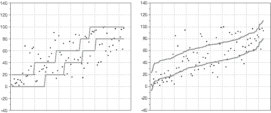
True plant height percentiles (•) and the intervals predicted (using a 10-fold cross validation) by nd(LR) with selection of features (left) and by metric regression (right) with ε = 15. To ease the readability, the horizontal axis represents the indexes of barley samples ordered according to their predictions. Notice that, therefore, the orderings of predictions in the horizontal axes are different in both pictures.

For plant height, the first attribute selected by the nondeterministic method is 2H(118.9); it is also reported as a relevant (QTL) for this trait by the methods SML, CIM and MR (Bedo et al., 2008). The merits of this attribute can be straightforwardly explained in a discretized phenotype setting. It provides a description of individuals from which it is possible to predict the right class 39% of times. Since the attribute is binary, it is only possible to reach a 40% of successful classifications; notice that it is only possible to produce 2 different predictions while the set of ranks has 5 elements. Therefore, 2H(118.9) is an almost perfect predictor. This classifier is telling us that all (with the exception of 1 sample) barleys with percentiles in (80, 100] have value 0 in 2H(118.9); and all barleys with percentiles in barleys [0, 20] have value 1 in 2H(118.9). This explanation can not be drawn from the report that the correlation of 2H(118.9) and the percentile of plant height is 0.65. In this context, correlation is quite opaque.

The top 5 features selected by our method are the following markers: 2H(118.9), 2H(0.0), 3H(117.4), 3H(74.5), and 5H(65.9). The first, third, and fifth attributes of this list are also reported as relevant (QTL) for this trait by the methods SML, CIM, and MR (Bedo et al., 2008). In general, it seems that a bit more sophisticated selection procedure (instead of a simple linear search) could remove some features from our list of QTLs. But we did not implement such a procedure in order to ensure scalability.

5. Conclusion

Once it is established that there is a genetic basis for a complex behavior expressed by a measurable phenotype, the aim is to explain this relationship in a useful way. In many important cases, phenotypes are represented by continuous numbers and then the genotype/phenotype relations can be typically explained using regression tools.

However, phenotypes are frequently influenced by environmental causes, and the joint action of many genetic features. In these cases, simple regression models provide predictors with poor performance. The approach presented here proposes to handle continuous phenotypes as approximations represented by intervals of percentiles. We have proved, in a real case, that the reliability of interval-valued predictors are considerably higher than that of point-valued regressors. We discussed two implementations of this idea. The first is based on regression with a loss function that uses a tolerance parameter ε. The second one discretizes the target values into a set of k bins of equal frequency, and then employs classifiers. However, the sizes of predicted intervals do not need to be the same for all genotypes, and this option can be incorporated if we use set-valued or nondeterministic classifiers: they may predict wider intervals for doubtful genotypes.

Additionally, handling phenotypes as approximations opens the possibility of using feature selectors of high performance, and whose complexity in terms of computation time is very low. In this sense, we have proved that deterministic classifiers can be delegated to select a set of features for nondeterministic tasks. Therefore, without heuristic jumps, we can use filters designed for deterministic classifiers to obtain a fully scalable method suitable for dealing with large genetic data sets.

Footnotes

Acknowledgments

We acknowledge those researchers who shared the barley data used in this article: Wenzl et al. (2006) and Bedo et al. (). This work was supported in part by the Spanish Ministerio de Ciencia e Innovacin (grant TIN2008-06247 to O.L., J.R.Q., J.D., J.J.C., and A.B.; and grant AGL2007-65563-C02-01/GAN to M.P.-E.).

Disclosure Statement

No competing financial interests exist.

References

Alonso

, del Coz

J.J.

, Díez

et al. 2008. Learning to predict one or more ranks in ordinal regression tasks. Lect. Notes Comput. Sci. I, 5211:39–54.

Bedo

, Wenzl

, Kowalczyk

et al. 2008. Precision-mapping and statistical validation of quantitative trait loci by machine learning. BMC Genet., 9:35.

Chang

C.-C.

, Lin

C.-J.

2001. LIBSVM: a library for support vector machines. www.csie.ntu.edu.tw/∼cjlin/libsvm. 2010 October 1.

Chu

, Keerthi

S.S.

2005. New approaches to support vector ordinal regression. Proc. ICML’05, 145–152.

Corani

, Zaffalon

2008. Learning reliable classifiers from small or incomplete data sets: the naive credal classifier 2. J. Mach. Learn. Res., 9:581–621.

del Coz

J.J.

, Díez

, Bahamonde

2009. Learning nondeterministic classifiers. J. Mach Learn Res, 10:2273–2293.

Lee

, van der Werf

, Hayes

et al. 2008. Predicting unobserved phenotypes for complex traits from whole-genome SNP data. PLoS Genet., 4:e1000231.

Lin

C.-J.

, Weng

R.C.

, Keerthi

S.S.

2008. Trust region Newton method for logistic regression. J. Mach. Learn. Res., 9:627–650.

Lynch

, Walsh

1998. Genetics and Analysis of Quantitative Traits. Sinauer: Sunderland, MA.

10.

Mauricio

2001. Mapping quantitative trait loci in plants: uses and caveats for evolutionary biology. Nat. Rev. Genet., 2:370–381.

11.

Meuwissen

, Hayes

, Goddard

2001. Prediction of total genetic value using genome-wide dense marker maps. Genetics, 157:1819–1829.

12.

Saeys

, Inza

, Larrañaga

2007. A review of feature selection techniques in bioinformatics. Bioinformatics, 23:2507–2517.

13.

Wenzl

, Li

, Carling

et al. 2006. A high-density consensus map of barley linking DArT markers to SSR, RFLP and STS loci and agricultural traits. BMC Genomics, 7:206.

14.

Wray

, Goddard

, Visscher

2007. Prediction of individual genetic risk to disease from genome-wide association studies. Genome Res, 17:1520–1528.

15.

, Liu

2004. Efficient feature selection via analysis of relevance and redundancy. J. Mach. Learn. Res., 5:1205–1224.