Exploratory Factor Analysis of Pathway Copy Number Data with an Application Towards the Integration with Gene Expression Data

Abstract

Realizing that genes often operate together, studies into the molecular biology of cancer shift focus from individual genes to pathways. In order to understand the regulatory mechanisms of a pathway, one must study its genes at all molecular levels. To facilitate such study at the genomic level, we developed exploratory factor analysis for the characterization of the variability of a pathway's copy number data. A latent variable model that describes the call probability data of a pathway is introduced and fitted with an EM algorithm. In two breast cancer data sets, it is shown that the first two latent variables of GO nodes, which inherit a clear interpretation from the call probabilities, are often related to the proportion of aberrations and a contrast of the probabilities of a loss and of a gain. Linking the latent variables to the node's gene expression data suggests that they capture the “global” effect of genomic aberrations on these transcript levels. In all, the proposed method provides an possibly insightful characterization of pathway copy number data, which may be fruitfully exploited to study the interaction between the pathway's DNA copy number aberrations and data from other molecular levels like gene expression.

1. Introduction

Cancer is a genetic disease, often caused by abnormalities in the genetic material of cancer cells (Hanahan and Weinberg, 2000). DNA copy number aberrations (CNAs), which are known to play a key role in the development and progression of cancer (Lengauer et al., 1998), are an example of such abnormalities. Among others, these CNAs may affect the expression levels of cancer genes. Cancer genes are genes that have the ability to direct malignant cell growth. However, no single gene “causes” cancer; only when several cancer genes work in concert may cancer develop (Vogelstein and Kinzler, 2004). It is therefore important to study the behavior of a pathway rather than that of individual genes. Such a study must be done at all molecular levels of the cell. For the genomic level, we present a method to characterize the variability in DNA copy number aberration patterns of the genes in a pathway.

CNAs are measured in a high-throughput fashion by array CGH (Pinkel and Albertson, 2005). In an array CGH experiment, differently labeled test (cancer) and reference samples are hybridized together to an array. The reference sample is assumed to have copy number two. Image analysis then results in test and reference intensities. The log₂ ratio of the test and reference intensities reflect the relative copy number in the test sample compared to that in the reference sample.

The array CGH data are pre-processed to arrive at an estimate of the copy number of a genomic segment. First, the log₂ ratios are normalized (Neuvial et al., 2006). Then, motivated by the underlying discrete DNA copy numbers of test and reference samples, change-point analysis techniques (Olshen et al., 2004) divide the genome into non-overlapping segments that are separated by breakpoints. These breakpoints indicate a change in DNA copy number, and consequently, the copy number does not change within a segment. In addition, the mean log₂ ratio of the segments is estimated. Due to the relativity of the measurement, the exact copy number of a segment cannot be determined; however, using mixture model approaches (Van de Wiel et al., 2007) deviations from the normal copy number can be detected. Each segment is then classified as either “normal,” “loss,” or “gain”—“normal” if there are two copies of the chromosomal segment present, “loss” if at least one copy is lost, and “gain” if at least one additional copy is present. These labels are referred to as calls. This classification is not perfect, for example, due to experimental noise or unknown contaminations by normal cells. To address this imperfection, the CNAs are represented by a vector of probabilities, one for each type of call that is discerned. Such probabilities reflect both cell heterogeneity and precision of the array CGH data. We refer to calls and these call probabilities also as “hard” and “soft” calls, respectively.

The potential of call probabilities in the analysis of array CGH data was suggested in Van Wieringen et al. (2007), and demonstrated in Van Wieringen and Van de Wiel (2009) and Gonzalez et al. (2009). Here, the use of call probabilities, through their clear interpretation, enables us to assign meaning (in terms of the copy numbers) to the characterization of a pathway's CNA patterns, which would be difficult when using the log₂ ratios. In turn, this meaning is crucial when linking the CNA patterns to, for example, gene expression if it is to provide understanding of this relationship.

We take the call probability signatures at the genomic locations of the genes in a pathway to constitute the copy number data of that pathway. Here a pathway is only a label for what is otherwise known as a gene set. A gene set is a collection of presumably related genes, for instance because they are believed to contribute to the same biological function. Gene set definitions are usually taken from repositories such as GO (Gene Ontology Consortium, 2000) or KEGG (Ogata et al., 1999). It is believed that analysis in terms of functionally related items facilitates the interpretation of results. Note however that such an analysis depends on the quality of the definition of the gene sets, which may have been compiled using incomplete, imperfect or incorrect information (Khatri and Draghici, 2005).

The study of CNAs in terms of pathways demands some justification, for regulatory mechanisms in a pathway are not described in terms of the genomic segments as defined by the breakpoints found in the array CGH experiment. Still, CNAs affect the transcriptome. They exert their influence through the entities (mRNAs, microRNAs, et cetera) that map to the segment. Among others, Pollack et al. (2002) showed the direct (univariate) effect of an increase (or decrease) in copy number on a gene's expression levels. However, genes often operate together (Vogelstein and Kinzler, 2004). Therefore, in order to advance our understanding of a pathway's regulatory mechanisms, one must study its genes at all molecular levels, also at the genomic level. This has been done in, for example, Valentijn et al. (2005) and Ferreira et al. (2008), who both show that copy number changes may affect the pathway's gene expression profile.

This article describes exploratory factor analysis (EFA) designed especially for the call probability array CGH data of a pathway. The EFA characterizes the variability in the CNA patterns by means of a number of latent variables. Hence, EFA is a dimension reduction technique, much like principal component analysis (PCA). PCA has been successfully used to characterize multivariate phenomena in gene expression data, and here we show that EFA has the same potential. Hereto we show that the clear interpretation of the call probabilities is transmitted to the latent variables. This helps to understand what is common and what is not—in terms of their CNA pathway profile—to the samples in the study. Such understanding may also be useful when exploring the effect of copy number changes (as captured by the latent variables) on gene expression levels in the pathway. In two breast cancer data sets, we show how the EFA characterizes copy number data of a GO node, and how it appears to capture the global effect of genomic aberrations on the node's gene expression levels.

1.1. Related work

As far as we are aware no method like exploratory factor analysis tailor-made for array CGH data has been proposed. We acknowledge that PCA could directly be applied to normalized or segmented log₂ ratio data, as is done by, for example, Somiari et al. (2004) and Unger et al. (2008). We therefore compare the proposed method to these approaches later and digress here on aspects that set them apart.

The fundamental difference between PCA and factor analysis is that the former does not assume a model for the data, whereas the latter does. This absence (or presence) of a model brings about other differences, for example, in components, eigenvectors (PCA) versus latent variables (EFA), and in the component construction algorithms, singular value decomposition (PCA) versus maximum likelihood type procedures (EFA). Despite their differences, PCA and factor analysis may produce similar results. See Schneeweiss and Mathes (1995) for an account of the mathematical conditions for their results to be similar. Apart from these methodological differences, the assumption of a model also has practical consequences: it facilitates (in combination with the interpretable call probabilities) the interpretation of latent variables. This is of crucial importance if the analysis is to provide insight into the biological phenomenon under study. Note that often (Alter et al., 2000) principal components are assigned interpretations as “eigengenes,” “supergenes,” or “meta-genes.” This interpretation is merely a label, for it is linked neither to a biological entity nor to a theoretical construct. The interpretation of principal components is generally not straightforward, especially if the number of features that contribute to the component gets large.

2. Methods

2.1. Model

Consider an experiment involving a sample of n cancers of a particular tissue. Associated with each cancer sample there is a copy number profile, which we take to consists of the call probabilities. Suppose pre-processing maps the raw array CGH data onto a scale with ordered categories \documentclass{aastex} \usepackage{amsbsy} \usepackage{amsfonts} \usepackage{amssymb} \usepackage{bm} \usepackage{mathrsfs} \usepackage{pifont} \usepackage{stmaryrd} \usepackage{textcomp} \usepackage{portland, xspace} \usepackage{amsmath, amsxtra} \pagestyle{empty} \DeclareMathSizes {10} {9} {7} {6} \begin{document} $$\{1, \ldots, a \}$$ \end{document} , with a the number of calls, corresponding to, say, {loss, normal, gain}. Then, the call probabilities reflect the certainty with which this is done. Let the call probabilities of sample i and feature j, \documentclass{aastex} \usepackage{amsbsy} \usepackage{amsfonts} \usepackage{amssymb} \usepackage{bm} \usepackage{mathrsfs} \usepackage{pifont} \usepackage{stmaryrd} \usepackage{textcomp} \usepackage{portland, xspace} \usepackage{amsmath, amsxtra} \pagestyle{empty} \DeclareMathSizes {10} {9} {7} {6} \begin{document} $$j = 1, \ldots, p$$ \end{document} with p the number of features in the pathway under study, be denoted by \documentclass{aastex} \usepackage{amsbsy} \usepackage{amsfonts} \usepackage{amssymb} \usepackage{bm} \usepackage{mathrsfs} \usepackage{pifont} \usepackage{stmaryrd} \usepackage{textcomp} \usepackage{portland, xspace} \usepackage{amsmath, amsxtra} \pagestyle{empty} \DeclareMathSizes {10} {9} {7} {6} \begin{document} $${\bf Q}_{i,\,j} = (Q_{i, j, 1, \ldots,}Q_{i, j, a})$$ \end{document} . Hence, \documentclass{aastex} \usepackage{amsbsy} \usepackage{amsfonts} \usepackage{amssymb} \usepackage{bm} \usepackage{mathrsfs} \usepackage{pifont} \usepackage{stmaryrd} \usepackage{textcomp} \usepackage{portland, xspace} \usepackage{amsmath, amsxtra} \pagestyle{empty} \DeclareMathSizes {10} {9} {7} {6} \begin{document} $$\sum \nolimits_{k = 1}^a Q_{i, j, k} = 1$$ \end{document} . The copy number matrix of a pathway is denoted as Q. We consider the call probabilities to be random variables themselves, although no assumptions regarding their distribution are made. This is motivated later.

We also assume the existence of m latent variables. These are introduced to reduce the dimensionality of the copy number data, as it is believed that the information/variability in the full data set can approximated/explained by a much smaller data set. The latent variables are denoted by \documentclass{aastex} \usepackage{amsbsy} \usepackage{amsfonts} \usepackage{amssymb} \usepackage{bm} \usepackage{mathrsfs} \usepackage{pifont} \usepackage{stmaryrd} \usepackage{textcomp} \usepackage{portland, xspace} \usepackage{amsmath, amsxtra} \pagestyle{empty} \DeclareMathSizes {10} {9} {7} {6} \begin{document} $${\bf Z}_i = (Z_{i, 1, \ldots,}Z_{i, m})$$ \end{document} for sample i.

We model the conditional expectation of the Q_i,j,k given the latent variables as: \documentclass{aastex} \usepackage{amsbsy} \usepackage{amsfonts} \usepackage{amssymb} \usepackage{bm} \usepackage{mathrsfs} \usepackage{pifont} \usepackage{stmaryrd} \usepackage{textcomp} \usepackage{portland, xspace} \usepackage{amsmath, amsxtra} \pagestyle{empty} \DeclareMathSizes {10} {9} {7} {6} \begin{document} \begin{align*} E_Q (Q_ {i, j, k} \mid {\bf Z} _i) = \theta_ {j, k} ({\bf Z} _i) = \frac {\exp \left(\alpha_ {j, k} + \sum_ {\ell = 1} ^m \beta_ {j, k, \ell} \ Z_ {i, \ell} \right)} {\sum_ {k = 1} ^a \exp \left(\alpha_ {j, k} + \sum_ {\ell = 1} ^m \beta_ {j, k, \ell} \ Z_ {i, \ell} \right)}. \tag {1} \end{align*} \end{document}

In the above model, α_j,k is the baseline log probability of call k for region j, and β_j,k,ℓ is the change in the kth log probability per unit change in latent variable ℓ for region j. We refer to the βs as the factor loadings. This model is identical to the generalized linear model used for nominal data (McCullagh and Nelder, 2000). Model (1) can also be considered to model the expectation of a Dirichlet distribution with parameters \documentclass{aastex} \usepackage{amsbsy} \usepackage{amsfonts} \usepackage{amssymb} \usepackage{bm} \usepackage{mathrsfs} \usepackage{pifont} \usepackage{stmaryrd} \usepackage{textcomp} \usepackage{portland, xspace} \usepackage{amsmath, amsxtra} \pagestyle{empty} \DeclareMathSizes {10} {9} {7} {6} \begin{document} $$\left(\exp \left(\alpha_{j, 1} + \sum \nolimits_{\ell = 1}^m \beta_{j, 1, \ell}\;Z_{i \ell} \right), \ldots, \exp \left(\alpha_{j, a} + \sum \nolimits_{\ell = 1}^m \beta_{j, a, \ell}\,Z_{i \ell} \right) \right).$$ \end{document}

To ensure all parameters in the model are estimable we set α_j,_normal = 0 = β_j,_normal,ℓ for all j and ℓ. For β_j,_normal,ℓ (similar reasoning applies to α_j,_normal) the need for this restriction becomes clear when studying the odds of call k₁ over call k₂, given by: \documentclass{aastex} \usepackage{amsbsy} \usepackage{amsfonts} \usepackage{amssymb} \usepackage{bm} \usepackage{mathrsfs} \usepackage{pifont} \usepackage{stmaryrd} \usepackage{textcomp} \usepackage{portland, xspace} \usepackage{amsmath, amsxtra} \pagestyle{empty} \DeclareMathSizes {10} {9} {7} {6} \begin{document} \begin{align*} \frac {E_Q (Q_ {i, j, k_1} \mid {\bf Z} _i)} {E_Q (Q_ {i, j, k_2} \mid {\bf Z} _i)} = \frac {\theta_ {j, k_1} ({\bf Z} _i)} {\theta_ {j, k_2} ({\bf Z} _i)} = \frac {\exp \left(\alpha_ {j, k_1} \right)} {\exp \left(\alpha_ {j, k_2} \right)} \exp \Bigg (\sum_ {\ell = 1} ^m (\beta_ {j, k_1, \ell} - \beta_ {j, k_2, \ell}) \ Z_ {i \ell} \Bigg). \end{align*} \end{document}

Thus, the contrast between the vectors \documentclass{aastex} \usepackage{amsbsy} \usepackage{amsfonts} \usepackage{amssymb} \usepackage{bm} \usepackage{mathrsfs} \usepackage{pifont} \usepackage{stmaryrd} \usepackage{textcomp} \usepackage{portland, xspace} \usepackage{amsmath, amsxtra} \pagestyle{empty} \DeclareMathSizes {10} {9} {7} {6} \begin{document} $$\beta_{j, k_1}$$ \end{document} and \documentclass{aastex} \usepackage{amsbsy} \usepackage{amsfonts} \usepackage{amssymb} \usepackage{bm} \usepackage{mathrsfs} \usepackage{pifont} \usepackage{stmaryrd} \usepackage{textcomp} \usepackage{portland, xspace} \usepackage{amsmath, amsxtra} \pagestyle{empty} \DeclareMathSizes {10} {9} {7} {6} \begin{document} $$\beta_{j, k_2}$$ \end{document} is of interest, not the vectors themselves. The imposed restriction changes the interpretation of (say) β_j,_gain,ℓ to the change in the log odds of a gain over a normal per unit change in latent variable ℓ for region j. Of course one may choose to set β_j,_gain,ℓ equal to zero. The normal call however seems the natural reference as all cancer cells (eventually) originate from a healthy cell with a normal copy number. In addition to the changed interpretation, the restriction leaves us with two parameters per latent variable: β_j,_loss,ℓ and β_j,_gain,ℓ. These distinguish between the different biological processes that lead to loss and gain, respectively, allowing different effects of the latent variable in both processes.

In the above, we have modeled the expectation of the call probabilities directly, and have refrained from specifying their distribution. Two obvious choices, as both are defined on the simplex, are the Dirichlet distribution (Kotz et al., 2000) and the logistic-normal distribution used for compositional data (Aitchison, 1992). Neither provides a reasonable description of the typical patterns of variability of the call probabilities. Figure 1 shows two examples of the distribution of call probabilities.

FIG. 1.

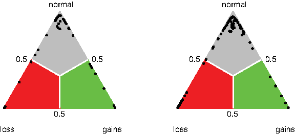
The distribution of call probability data on the simplex of two features.

In call probability data the majority of data points falls on the nodes and edges of the simplex. This is due to the fact that the log₂ ratios often clearly indicate (say) a gain. If there is uncertainty in the calling, it is between adjacent calls for example, between normal and gain. A small number of data points falls a little more in the interior of the simplex, corresponding to a probability mass slightly more equally distributed over all calls. This is likely to be due to cell heterogeneity and noisy array elements. Note that the fact that there are no observations near the points \documentclass{aastex} \usepackage{amsbsy} \usepackage{amsfonts} \usepackage{amssymb} \usepackage{bm} \usepackage{mathrsfs} \usepackage{pifont} \usepackage{stmaryrd} \usepackage{textcomp} \usepackage{portland, xspace} \usepackage{amsmath, amsxtra} \pagestyle{empty} \DeclareMathSizes {10} {9} {7} {6} \begin{document} $$\left(\frac {1} {3}, \frac {1} {3}, \frac {1} {3} \right)$$ \end{document} or \documentclass{aastex} \usepackage{amsbsy} \usepackage{amsfonts} \usepackage{amssymb} \usepackage{bm} \usepackage{mathrsfs} \usepackage{pifont} \usepackage{stmaryrd} \usepackage{textcomp} \usepackage{portland, xspace} \usepackage{amsmath, amsxtra} \pagestyle{empty} \DeclareMathSizes {10} {9} {7} {6} \begin{document} $$\left(\frac {1} {2}, 0, \frac {1} {2} \right)$$ \end{document} is due to the design of the measurement which takes the normal copy number as a reference. Biologically, it may well be possible for a sample to contain genomic segments that are primarily aberrated in the cells from which the hybridized DNA was extracted, but lost in some cells and gained in others. It has been suggested (Aitchison, 1992) to model situations with many points falling on the simplex’ edges by a mixture of distributions, possibly defined on lower dimensional simplexes. This however brings about issues with respect to the number of components and the type of distributions in the mixture that need to be resolved. In addition, it will involve more parameters that also need to be estimated. We consider these issues beyond the scope of this initial paper on factor analysis of array CGH data and save them for further research.

Focusing on a single array element still, the unconditional expectation of Q_i,j,k is: \documentclass{aastex} \usepackage{amsbsy} \usepackage{amsfonts} \usepackage{amssymb} \usepackage{bm} \usepackage{mathrsfs} \usepackage{pifont} \usepackage{stmaryrd} \usepackage{textcomp} \usepackage{portland, xspace} \usepackage{amsmath, amsxtra} \pagestyle{empty} \DeclareMathSizes {10} {9} {7} {6} \begin{document} \begin{align*} E_Z (E_Q (Q_{i, j, k} \mid {\bf Z}_i)) = \int_{- \infty}^{\infty} \ldots \int_{- \infty}^{\infty} E_Q (Q_{i, j, k} \mid {\bf Z}) \; f ({\bf Z}) \;d{\bf Z} \end{align*} \end{document}

where f the density of the Z. Following Jöreskog and Moustaki (2001), who discuss factor analysis of ordinal data (hard calls), the latent variables Z_i,ℓ are assumed to be independent with standard normal distributions. Then, rewriting, \documentclass{aastex} \usepackage{amsbsy} \usepackage{amsfonts} \usepackage{amssymb} \usepackage{bm} \usepackage{mathrsfs} \usepackage{pifont} \usepackage{stmaryrd} \usepackage{textcomp} \usepackage{portland, xspace} \usepackage{amsmath, amsxtra} \pagestyle{empty} \DeclareMathSizes {10} {9} {7} {6} \begin{document} \begin{align*} E_Z (E_Q (Q_{i, j, k} \mid {\bf Z}_i)) = \int_{- \infty}^{\infty} \ldots \int_{- \infty}^{\infty} E_Q (Q_{i, j, k} \mid {\bf Z}) \prod_{\ell = 1}^m \phi_{0, 1} (Z_{\ell})\; d Z_1 \ldots d Z_m. \end{align*} \end{document}

Assuming the latent variable distribution to be independent standard normal removes the indeterminancy of the model only up to a rotation.

For any rotation matrix R, we have (using R^T R = I): \documentclass{aastex} \usepackage{amsbsy} \usepackage{amsfonts} \usepackage{amssymb} \usepackage{bm} \usepackage{mathrsfs} \usepackage{pifont} \usepackage{stmaryrd} \usepackage{textcomp} \usepackage{portland, xspace} \usepackage{amsmath, amsxtra} \pagestyle{empty} \DeclareMathSizes {10} {9} {7} {6} \begin{document} \begin{align*} E_Q (Q_ {i, j, k} \mid {\bf Z} _i) = \frac {\exp \big (\alpha_ {j, k} + {\beta} _ {j, k} ^T \ {\bf Z} _ {i} \big)} {\sum_ {k = 1} ^a \exp \big (\alpha_ {j, k} + {\bf \beta} _ {j, k} ^T \ {\bf Z} _ {i} \big)} = \frac {\exp \big (\alpha_ {j, k} + ({\bf R} {\bf \beta} _ {j, k}) ^T \ {\bf R} {\bf Z} _ {i} \big)} {\sum_ {k = 1} ^a \exp \big (\alpha_ {j, k} + ({\bf R} {\bf \beta} _ {j, k}) ^T \ {\bf R} {\bf Z} _ {i} \big)}, \end{align*} \end{document}

making the corresponding models indistinguishable. This indeterminancy is common to all latent variable models (Bartholomew and Knott, 1999), and is irrelevant for the purpose of low-dimensional plotting, as most statistical software packages allow the user to rotate the axis in order to find an angle of his or her liking. However, the choice of rotation matrix affects the interpretation of the latent variables as brought forth by the factor loadings, but this choice should be made on non-statistical grounds as all rotations fit the data equally well.

2.2. Parameter estimation

The parameters of model (1) are estimated by minimizing the following loss function: \documentclass{aastex} \usepackage{amsbsy} \usepackage{amsfonts} \usepackage{amssymb} \usepackage{bm} \usepackage{mathrsfs} \usepackage{pifont} \usepackage{stmaryrd} \usepackage{textcomp} \usepackage{portland, xspace} \usepackage{amsmath, amsxtra} \pagestyle{empty} \DeclareMathSizes {10} {9} {7} {6} \begin{document} \begin{align*} {\cal L}_m = - \sum_{i = 1}^n \log \Bigg (\int_{- \infty}^{\infty} \ldots \int_{- \infty}^{\infty} \prod_{j = 1}^p \prod_{k = 1}^a E (Q_{i, j, k} \mid {\bf Z}) ^{Q_{i, j, k}} \prod_{\ell = 1}^m \phi_{0, 1} (Z_{\ell}) \ d Z_1 \ldots d Z_m \Bigg) \tag{2} \end{align*} \end{document}

This loss function can be motivated by further pursuing the analogy with nominal data modeling (briefly mentioned in the previous section). Would the calling process have been perfect, the calls are determined without uncertainty, resulting in hard calls (instead of soft calls). In the present notation, the call probability data Q_i,j become unit vectors, for instance, (1, 0, 0) for a loss (interpretation: a probability of a loss equal to one). Such data may be assumed to be a realization of one draw from a multinomial process, with parameters \documentclass{aastex} \usepackage{amsbsy} \usepackage{amsfonts} \usepackage{amssymb} \usepackage{bm} \usepackage{mathrsfs} \usepackage{pifont} \usepackage{stmaryrd} \usepackage{textcomp} \usepackage{portland, xspace} \usepackage{amsmath, amsxtra} \pagestyle{empty} \DeclareMathSizes {10} {9} {7} {6} \begin{document} $$(\theta_{j, 1} ({\bf Z}_i), \ldots, \theta_{j, a} ({\bf Z}))$$ \end{document} . Combining this multinomial model with conditional independence between the array elements in the pathway and the assumption of independent, normally distributed latent variables, one arrives at a log-likelihood function proportional to the proposed loss function.

We evaluate the integral in (2) by the Gauss-Hermite quadrature approximation: \documentclass{aastex} \usepackage{amsbsy} \usepackage{amsfonts} \usepackage{amssymb} \usepackage{bm} \usepackage{mathrsfs} \usepackage{pifont} \usepackage{stmaryrd} \usepackage{textcomp} \usepackage{portland, xspace} \usepackage{amsmath, amsxtra} \pagestyle{empty} \DeclareMathSizes {10} {9} {7} {6} \begin{document} \begin{align*} & \int_{- \infty}^{\infty} \ldots \int_{- \infty}^{\infty} \prod_{j = 1}^p \prod_{k = 1}^a E (Q_{i, j, k} \mid {\bf Z}) ^{Q_{i, j, k}} \prod_{\ell = 1}^m \phi_{0, 1} (Z_{\ell}) \ d Z_1 \ldots d Z_m \\ & \simeq \sum_{g_1 = 1}^{G_1} \ldots \sum_{g_m = 1}^{G_m} h (z_{g_1}) \cdot \ldots \cdot h (z_{g_m}) \prod_{j = 1}^p \prod_{k = 1}^a \theta_{j, k} (z_{g_1}, \ldots, z_{g_m}) ^{Q_{i, j, k}} \end{align*} \end{document}

where the \documentclass{aastex} \usepackage{amsbsy} \usepackage{amsfonts} \usepackage{amssymb} \usepackage{bm} \usepackage{mathrsfs} \usepackage{pifont} \usepackage{stmaryrd} \usepackage{textcomp} \usepackage{portland, xspace} \usepackage{amsmath, amsxtra} \pagestyle{empty} \DeclareMathSizes {10} {9} {7} {6} \begin{document} $$z_{g_ \ell}$$ \end{document} are the abscissas of the quadrature and \documentclass{aastex} \usepackage{amsbsy} \usepackage{amsfonts} \usepackage{amssymb} \usepackage{bm} \usepackage{mathrsfs} \usepackage{pifont} \usepackage{stmaryrd} \usepackage{textcomp} \usepackage{portland, xspace} \usepackage{amsmath, amsxtra} \pagestyle{empty} \DeclareMathSizes {10} {9} {7} {6} \begin{document} $$h (z_{g_ \ell})$$ \end{document} the corresponding weights. In effect, the latent variable is discretized having values \documentclass{aastex} \usepackage{amsbsy} \usepackage{amsfonts} \usepackage{amssymb} \usepackage{bm} \usepackage{mathrsfs} \usepackage{pifont} \usepackage{stmaryrd} \usepackage{textcomp} \usepackage{portland, xspace} \usepackage{amsmath, amsxtra} \pagestyle{empty} \DeclareMathSizes {10} {9} {7} {6} \begin{document} $$z_1, \ldots, z_{G_ \ell}$$ \end{document} with probabilities \documentclass{aastex} \usepackage{amsbsy} \usepackage{amsfonts} \usepackage{amssymb} \usepackage{bm} \usepackage{mathrsfs} \usepackage{pifont} \usepackage{stmaryrd} \usepackage{textcomp} \usepackage{portland, xspace} \usepackage{amsmath, amsxtra} \pagestyle{empty} \DeclareMathSizes {10} {9} {7} {6} \begin{document} $$h (z_1), \ldots, h (z_{G_ \ell})$$ \end{document} which satisfy \documentclass{aastex} \usepackage{amsbsy} \usepackage{amsfonts} \usepackage{amssymb} \usepackage{bm} \usepackage{mathrsfs} \usepackage{pifont} \usepackage{stmaryrd} \usepackage{textcomp} \usepackage{portland, xspace} \usepackage{amsmath, amsxtra} \pagestyle{empty} \DeclareMathSizes {10} {9} {7} {6} \begin{document} $$\sum \nolimits_{g \ell = 1}^{G_ \ell} h (z_{g_ \ell}) = 1$$ \end{document} . The integral can be approximated to any desired degree of accuracy by increasing the number of quadrature points.

The parameters are now estimated by minimizing the Gauss-Hermite quadrature approximated loss function. This is done through the application of a modified version of the EM-algorithm proposed in Qu et al. (1996), where it is used to fit a latent variable model to binary data. The EM algorithm as applied to the present situation can be described as follows:

Step 1. Choose initial values for the estimate \documentclass{aastex} \usepackage{amsbsy} \usepackage{amsfonts} \usepackage{amssymb} \usepackage{bm} \usepackage{mathrsfs} \usepackage{pifont} \usepackage{stmaryrd} \usepackage{textcomp} \usepackage{portland, xspace} \usepackage{amsmath, amsxtra} \pagestyle{empty} \DeclareMathSizes {10} {9} {7} {6} \begin{document} $$({\hat{\boldsymbol \alpha}}^{(0)}, {\hat{\boldsymbol \beta}}^{(0)})$$ \end{document} . In addition, specify a stopping criterion. Stopping criteria usually specify a maximum number of iterations or a minimum distance between two successive iterations that is to be achieved.

Step 2 (E-step). Calculate, using the current parameter estimates \documentclass{aastex} \usepackage{amsbsy} \usepackage{amsfonts} \usepackage{amssymb} \usepackage{bm} \usepackage{mathrsfs} \usepackage{pifont} \usepackage{stmaryrd} \usepackage{textcomp} \usepackage{portland, xspace} \usepackage{amsmath, amsxtra} \pagestyle{empty} \DeclareMathSizes {10} {9} {7} {6} \begin{document} $$({\hat{\boldsymbol \alpha}}^{(t)}, {\hat{\boldsymbol \beta}}^{(t)})$$ \end{document} : \documentclass{aastex} \usepackage{amsbsy} \usepackage{amsfonts} \usepackage{amssymb} \usepackage{bm} \usepackage{mathrsfs} \usepackage{pifont} \usepackage{stmaryrd} \usepackage{textcomp} \usepackage{portland, xspace} \usepackage{amsmath, amsxtra} \pagestyle{empty} \DeclareMathSizes {10} {9} {7} {6} \begin{document} \begin{align*} r_ {i, g_1, \ldots, g_m} ^ {(t)} = \frac {h (z_ {g_1}) \cdot \ldots \cdot h (z_ {g_m}) \prod_ {j = 1} ^p \prod_ {k = 1} ^a \theta_ {j, k} (z_ {g_1}, \ldots, z_ {g_m}) ^ {Q_ {i, j, k}}} {\sum_ {g_1 = 1} ^ {G_1} \ldots \sum_ {g_m = 1} ^ {G_m} h (z_ {g_1}) \cdot \ldots \cdot h (z_ {g_m}) \prod_ {j = 1} ^p \prod_ {k = 1} ^a \theta_ {j, k} (z_ {g_1}, \ldots, z_ {g_m}) ^ {Q_ {i, j, k}}}, \end{align*} \end{document}

which could (loosely) be interpreted as being (proportional to) the posterior probability of observing call probability profile Q_i at quadrature point \documentclass{aastex} \usepackage{amsbsy} \usepackage{amsfonts} \usepackage{amssymb} \usepackage{bm} \usepackage{mathrsfs} \usepackage{pifont} \usepackage{stmaryrd} \usepackage{textcomp} \usepackage{portland, xspace} \usepackage{amsmath, amsxtra} \pagestyle{empty} \DeclareMathSizes {10} {9} {7} {6} \begin{document} $$(z_{g_1}, \ldots, z_{g_m})$$ \end{document} .

Step 3 (M-step). Find, per array element in the pathway, the zero's of the first order partial derivatives of the loss function (see Supplementary Material for the derivation; all Supplementary Material is available at www.liebertonline.com/cmb): \documentclass{aastex} \usepackage{amsbsy} \usepackage{amsfonts} \usepackage{amssymb} \usepackage{bm} \usepackage{mathrsfs} \usepackage{pifont} \usepackage{stmaryrd} \usepackage{textcomp} \usepackage{portland, xspace} \usepackage{amsmath, amsxtra} \pagestyle{empty} \DeclareMathSizes {10} {9} {7} {6} \begin{document} \begin{align*} & \qquad - \sum_{i = 1}^n \sum_{g_1 = 1}^{G_1} \ldots \sum_{g_m = 1}^{G_m} r_{i, g_1, \ldots, g_m}^{(t)} \Big [Q_{i, j_0, k_0} - \theta_{j_0, k_0} (z_{g_1}, \ldots, z_{g_m}) \Big ] = 0, \\ & - \sum_{i = 1}^n \sum_{g_1 = 1}^{G_1} \ldots \sum_{g_m = 1}^{G_m} r_{i, g_1, \ldots, g_m}^{(t)} z_{g_{\ell_0}} \ \Big [Q_{i, j_0, k_0} - \theta_{j_0, k_0} (z_{g_1}, \ldots, z_{g_m}) \Big] = 0, \end{align*} \end{document}

with respect to the parameters \documentclass{aastex} \usepackage{amsbsy} \usepackage{amsfonts} \usepackage{amssymb} \usepackage{bm} \usepackage{mathrsfs} \usepackage{pifont} \usepackage{stmaryrd} \usepackage{textcomp} \usepackage{portland, xspace} \usepackage{amsmath, amsxtra} \pagestyle{empty} \DeclareMathSizes {10} {9} {7} {6} \begin{document} $$({\boldsymbol \alpha}_{j_0}, {\boldsymbol \beta}_{j_0})$$ \end{document} , which only appear in term \documentclass{aastex} \usepackage{amsbsy} \usepackage{amsfonts} \usepackage{amssymb} \usepackage{bm} \usepackage{mathrsfs} \usepackage{pifont} \usepackage{stmaryrd} \usepackage{textcomp} \usepackage{portland, xspace} \usepackage{amsmath, amsxtra} \pagestyle{empty} \DeclareMathSizes {10} {9} {7} {6} \begin{document} $$\theta_{{j_0}, {k_0}} (z_{g_1}, \ldots, z_{g_m})$$ \end{document} . This yields the new parameter estimates \documentclass{aastex} \usepackage{amsbsy} \usepackage{amsfonts} \usepackage{amssymb} \usepackage{bm} \usepackage{mathrsfs} \usepackage{pifont} \usepackage{stmaryrd} \usepackage{textcomp} \usepackage{portland, xspace} \usepackage{amsmath, amsxtra} \pagestyle{empty} \DeclareMathSizes {10} {9} {7} {6} \begin{document} $$({\hat{\boldsymbol \alpha}}^{(t + 1)}, {\hat{\boldsymbol \beta}}^{(t + 1)})$$ \end{document} .

Step 4. Go back to Step 2 until the stopping criterion has been satisfied.

The algorithm is initialized with \documentclass{aastex} \usepackage{amsbsy} \usepackage{amsfonts} \usepackage{amssymb} \usepackage{bm} \usepackage{mathrsfs} \usepackage{pifont} \usepackage{stmaryrd} \usepackage{textcomp} \usepackage{portland, xspace} \usepackage{amsmath, amsxtra} \pagestyle{empty} \DeclareMathSizes {10} {9} {7} {6} \begin{document} $${\hat{\boldsymbol \alpha}}^{(0)}$$ \end{document} equal to the logarithm of the first order moments fitted for each region, and the \documentclass{aastex} \usepackage{amsbsy} \usepackage{amsfonts} \usepackage{amssymb} \usepackage{bm} \usepackage{mathrsfs} \usepackage{pifont} \usepackage{stmaryrd} \usepackage{textcomp} \usepackage{portland, xspace} \usepackage{amsmath, amsxtra} \pagestyle{empty} \DeclareMathSizes {10} {9} {7} {6} \begin{document} $${\hat{\boldsymbol \beta}}^{(0)}$$ \end{document} drawn from a normal distribution.

To assess whether this estimation procedure is capable of reconstructing the latent variables, we conducted a small simulation study (see Supplementary Material). This shows that the Spearman's rank correlation between the “true” factors and their estimated counterparts is close to either one or minus one (the latter is due to the fact that the model is determined up to a rotation).

As with most optimization methods, the above algorithm may converge to local minima. It may therefore be useful to run it several times, the random choice of the initial βs warrants different initial values. It is our experience that the algorithm is quite stable, converging to the same minimum (see Supplementary Material).

2.3. Estimation and interpretation of the factors

Having obtained an estimate of the parameters \documentclass{aastex} \usepackage{amsbsy} \usepackage{amsfonts} \usepackage{amssymb} \usepackage{bm} \usepackage{mathrsfs} \usepackage{pifont} \usepackage{stmaryrd} \usepackage{textcomp} \usepackage{portland, xspace} \usepackage{amsmath, amsxtra} \pagestyle{empty} \DeclareMathSizes {10} {9} {7} {6} \begin{document} $$({\hat{\boldsymbol \alpha}}, {\hat{\boldsymbol \beta}})$$ \end{document} , the factor score of sample i with respect to latent variable \documentclass{aastex} \usepackage{amsbsy} \usepackage{amsfonts} \usepackage{amssymb} \usepackage{bm} \usepackage{mathrsfs} \usepackage{pifont} \usepackage{stmaryrd} \usepackage{textcomp} \usepackage{portland, xspace} \usepackage{amsmath, amsxtra} \pagestyle{empty} \DeclareMathSizes {10} {9} {7} {6} \begin{document} $$\ell, Z_{i, \ell}$$ \end{document} , is estimated by: \documentclass{aastex} \usepackage{amsbsy} \usepackage{amsfonts} \usepackage{amssymb} \usepackage{bm} \usepackage{mathrsfs} \usepackage{pifont} \usepackage{stmaryrd} \usepackage{textcomp} \usepackage{portland, xspace} \usepackage{amsmath, amsxtra} \pagestyle{empty} \DeclareMathSizes {10} {9} {7} {6} \begin{document} \begin{align*} \hat {Z} _ {i, \ell} = \frac {\sum_ {g_1 = 1} ^ {G_1} \ldots \sum_ {g_m = 1} ^ {G_m} z_ {g_ \ell} h (z_ {g_1}) \cdot \ldots \cdot h (z_ {g_m}) \prod_ {j = 1} ^p \prod_ {k = 1} ^a \theta_ {j, k} (z_ {g_1}, \ldots, z_ {g_m}) ^ {Q_ {i, j, k}}} {\sum_ {g_1 = 1} ^ {G_1} \ldots \sum_ {g_m = 1} ^ {G_m} h (z_ {g_1}) \cdot \ldots \cdot h (z_ {g_m}) \prod_ {j = 1} ^p \prod_ {k = 1} ^a \theta_ {j, k} (z_ {g_1}, \ldots, z_ {g_m}) ^ {Q_ {i, j, k}}}, \end{align*} \end{document}

which (again) is derived in analogy to the multinomial situation, where it would correspond to posterior expectation.

To assign interpretation to the latent factors we have found the following procedures useful:

Plot the factor scores of the latent variable against a contrast of call probabilities like \documentclass{aastex} \usepackage{amsbsy} \usepackage{amsfonts} \usepackage{amssymb} \usepackage{bm} \usepackage{mathrsfs} \usepackage{pifont} \usepackage{stmaryrd} \usepackage{textcomp} \usepackage{portland, xspace} \usepackage{amsmath, amsxtra} \pagestyle{empty} \DeclareMathSizes {10} {9} {7} {6} \begin{document} $$\sum \nolimits_{j = 1}^p Q_{i, j, \hbox{gain}} + \sum \nolimits_{j = 1}^p Q_{i, j, \hbox{loss \rm or}} \sum \nolimits_{j = 1}^p Q_{i, j, \hbox{gain}} - \sum \nolimits_{j = 1}^p Q_{i, j, \hbox{loss}}$$ \end{document} . The contrast may be limited to a subset of the features. The resulting plot may reveal whether the latent factor is associated with a particular aberration pattern (see Supplementary Material).

Select, e.g., four samples, two with the highest and two with the lowest factor score of a latent variable. Compare their call probability profiles. Differences in aberration patterns between the samples with the high and low factor scores may be related to the studied latent variable (see Supplementary Material).

In our experience, based on the analysis of multiple data sets, almost always one factor is highly correlated with the proportion of aberrations (or the like) of the samples. The other factors are more complicated to interpret but seem often to be related to a contrast in aberrations of a particular genomic segment.

The interpretation is however dependent on the rotation chosen. This is irrelevant for the situation with one latent variable. Also for m = 2, as almost always one factor is related to the percentage of aberrations, the rotation is fixed up to symmetry, and consequently the interpretation is fixed. For three (or more) latent variables, one still has a degree of freedom in the rotation. In such cases, to facilitate easy interpretation, the rotation is often chosen to maximize the variance of the (standardized) factor loadings. This results in factor loadings being either close to zero or being away from zero. The latent variable then only has to be interpreted in terms of the features corresponding to the latter as they have the largest contribution to the latent variable. Note however that the larger the number of factors (three and higher), the more difficult to endow all of them with a clear interpretation.

2.4. Ranking

In the event that one studies not a particular pathway but many pathways simultaneously, it is of interest to rank those that are best characterized by the results of the exploratory factor analysis. Hereto we present two statistics both measuring the quality of the EFA characterization that can be used to rank the pathways. The first criterion is the loss reduction (LR) obtained by minimizing (2): \documentclass{aastex} \usepackage{amsbsy} \usepackage{amsfonts} \usepackage{amssymb} \usepackage{bm} \usepackage{mathrsfs} \usepackage{pifont} \usepackage{stmaryrd} \usepackage{textcomp} \usepackage{portland, xspace} \usepackage{amsmath, amsxtra} \pagestyle{empty} \DeclareMathSizes {10} {9} {7} {6} \begin{document} \begin{align*} LR = \frac {1} {n} ({\cal L} _0 ({\bf Q}; {\hat {\boldsymbol \alpha}}) - {\cal L} _m ({\bf Q}; {\hat {\boldsymbol \alpha}}, {\hat {\boldsymbol \beta}})), \end{align*} \end{document}

where \documentclass{aastex} \usepackage{amsbsy} \usepackage{amsfonts} \usepackage{amssymb} \usepackage{bm} \usepackage{mathrsfs} \usepackage{pifont} \usepackage{stmaryrd} \usepackage{textcomp} \usepackage{portland, xspace} \usepackage{amsmath, amsxtra} \pagestyle{empty} \DeclareMathSizes {10} {9} {7} {6} \begin{document} $${\cal L}_0 ({\bf Q}; {\hat{\boldsymbol \alpha}})$$ \end{document} is the loss under the null model with no latent factors. An alternative ranking criterion would be the Kullback-Leibler divergence, defined as the difference in cross-entropy of the fitted and null model: CE_null − CE_fitted, where: \documentclass{aastex} \usepackage{amsbsy} \usepackage{amsfonts} \usepackage{amssymb} \usepackage{bm} \usepackage{mathrsfs} \usepackage{pifont} \usepackage{stmaryrd} \usepackage{textcomp} \usepackage{portland, xspace} \usepackage{amsmath, amsxtra} \pagestyle{empty} \DeclareMathSizes {10} {9} {7} {6} \begin{document} \begin{align*} CE = - \frac {1} {n p} \sum_ {i = 1} ^n \sum_ {j = 1} ^p \sum_ {k = 1} ^a Q_ {i, j, k} \log (g (Q_ {i, j, k})), \tag {3} \end{align*} \end{document}

which measures the discrepancy between the observed call probability data and a distribution g(Q_i,j,k). The cross-entropy between the data and the fitted model (CE_fitted) is calculated by replacing g(Q_i,j,k) by \documentclass{aastex} \usepackage{amsbsy} \usepackage{amsfonts} \usepackage{amssymb} \usepackage{bm} \usepackage{mathrsfs} \usepackage{pifont} \usepackage{stmaryrd} \usepackage{textcomp} \usepackage{portland, xspace} \usepackage{amsmath, amsxtra} \pagestyle{empty} \DeclareMathSizes {10} {9} {7} {6} \begin{document} $$E (Q_{i, j, k} \mid \hat{Z}_{i}; {\hat{\boldsymbol \alpha}}, \hat{\beta})$$ \end{document} into Equation (3). Similarly, for the null model with no latent factors substitute \documentclass{aastex} \usepackage{amsbsy} \usepackage{amsfonts} \usepackage{amssymb} \usepackage{bm} \usepackage{mathrsfs} \usepackage{pifont} \usepackage{stmaryrd} \usepackage{textcomp} \usepackage{portland, xspace} \usepackage{amsmath, amsxtra} \pagestyle{empty} \DeclareMathSizes {10} {9} {7} {6} \begin{document} $$g ({\bf Q}_{i, j, k}) = E (Q_{i, j, k} \mid \hat{\alpha})$$ \end{document} into the cross-entropy definition, which is denoted CE_null. Well-characterized pathways are those with a high loss reduction or Kullback-Leibler divergence. These statistics in combination with re-sampling may be used to develop a test to assess whether the loss reduction or Kullback-Leibler divergence is substantial.

3. Illustrations

The potential of the proposed method is illustrated by an exploratory study of two breast cancer data sets published by Pollack et al. (2002) and Bergamaschi et al. (2006). Henceforth, we refer to the data sets by the name of the first author (e.g., the Pollack data set). The Pollack and Bergamaschi data sets comprises of copy number and gene expression profiles, measured on cDNA microarray platforms, of 41 and 85 primary breast tumors (see Supplementary Material for pre-processing details). The gene expression of both data sets is used to investigate the link between the latent factors of a pathway's copy number data and its expression levels.

3.1. Characterization of the first two factors

First we investigate whether the interpretation of the two first EFA factors (the proportion of aberrations and the difference between the proportion of gains minus that of losses) as illustrated in Section 2.3 upholds more generally. Hereto we randomly selected 250 non-trivial (containing more than 20 gene and at most a 100 to exclude trivial and non-specific GO nodes, respectively) biological process category GO nodes. To the CNA data from each selected GO node, we fitted a two-factor model and estimated each sample's factor scores, its proportion of aberrations and its gain-vs-loss contrast. Spearman's rank correlations between the estimated factor scores and proportion and contrast for all GO nodes are calculated.

Figure 2 shows histograms of the absolute value of the Spearman's rank correlations. The upper panels show that the first EFA factor of a clear majority of GO nodes is highly correlated with the proportion of aberrations (Pollack: q_0.25 = 0.88 and q_0.50 = 0.93; Bergamaschi: q_0.25 = 0.81 and q_0.50 = 0.87). This observation does not come as a surprise. Bergamaschi and co-workers already noted that genome-wide the basal breast cancer subtype (as defined in Perou et al., 2000) is associated with a larger number of aberrations than other subtypes. Hence, as also the Pollack data set most likely (this information is not available) consists of all subtypes, one expects many GO nodes to reflect the genome-wide behavior: samples are distinguishable by their proportion of aberrations (the first EFA factor).

FIG. 2.

(Left) Histogram of the absolute Spearman correlation between the first factor and the number of aberrations. (Right) Same correlation plotted against the GO node size.

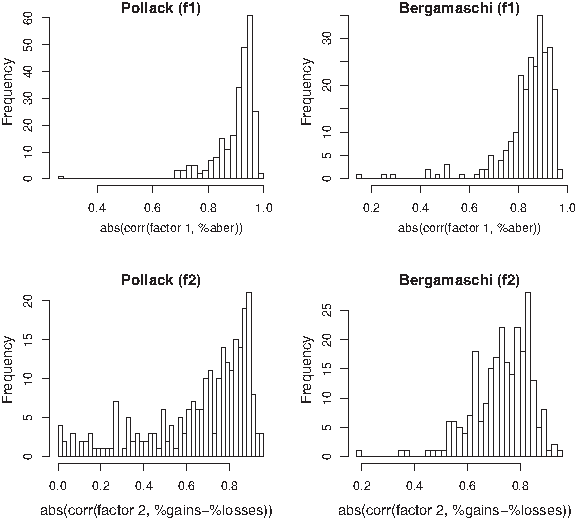
The lower panels of Figure 2 reveal that for a clear majority of the GO nodes the second EFA factor correlates with the contrast of gains and losses (Pollack: q_0.25 = 0.61 and q_0.50 = 0.78; Bergamaschi: q_0.25 = 0.68 and q_0.75 = 0.87). This contrast has not been noticed by Bergamaschi et al. (2006) as a characteristic separating the subtypes. In fact, Section 3.2 contains an example of a GO node where the latent factors reasonably separate the breast cancer subtypes basal from non-basal. Oddly enough, it is not the first factor, which correlates strongly with the proportion of aberrations, that is responsible for the separation, but the second factor, which correlates with the gain-vs-loss contrast. This is contrary to what was to be expected from the observation of Bergamaschi et al. (2006). EFA may thus give more subtle, specific information on a GO pathway's main characteristics than may be deduced from the genome-wide observation of Bergamaschi et al. (2006).

The above is of course no warrant that the two observed interpretations will always yield a good characterization of a pathway's copy number data variability. Associations may be of a weaker nature than observed here. In addition, the contrasts limited to a subset of the features in the pathway may yield a better association. This may also be the case for contrast between the percentages of non-gains and gains (or losses and non-losses), instead of between percentages of losses and gains. An example of a different interpretation than the above is given in Section 3.3, where the first factor is in fact correlated with the proportion of gains and the second with the proportion of losses.

3.2. Low-dimensional plotting

The latent variables may be used for low-dimensional plotting. In a plot, where each axis represents a latent variable, the estimated factor score vector of each sample is plotted. The samples are labeled in accordance with a clinical parameter. If the plot reveals that different values of the clinical parameter occupy different parts of the latent space, it seems possible to separate the samples with different clinical parameter values on the basis of the latent variables. An illustration is given in the left panel of Figure 3, where the latent factors reasonably separate the breast cancer subtypes (as defined in Perou et al., 2000) basal from non-basal. Another use of low dimensional plotting is to find corroboration of the sample subgroups found by (say) hierarchical clustering through an independent statistical technique, common practice in the analysis of gene expression data, for example, LaPointe et al. (2004). This is illustrated in the middle and right panel of Figure 3. The samples are clustered hierarchically using the average symmetric Kullback-Leibler divergence as a distance measure in combination with Ward's linkage (see Supplementary Material). The hard calls (instead of soft calls) are plotted in the heatmaps. The color bars above the heatmaps depict the two factor scores. Both factors are cut at their median and lower and upper 50% of the data are colored differently. This already indicates that the clustering may be explained by means of the latent factors, and is confirmed by the low dimensional plot in which the clusters separate reasonably well.

FIG. 3.

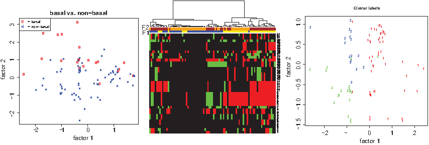
Heatmap and low-dimensional plots.

In principle the proposed method may be applied directly to copy number data from the whole genome (as opposed to that of a pathway), as is common in the analysis of gene expression data. We would then minimize the loss function over data from the whole genome. This practice may be acceptable as we are—in a strict sense—not working in a likelihood framework. It is also somewhat questionable as whole genome data are likely to violate the conditional independence assumption between features that is implicitly used in the motivation of the loss function. For there is a large redundancy in the data: many contiguous features have identical call probability signatures. Within these (possibly large) blocks of similar behaving features, the conditional independence assumption does not hold. An obvious way out would be to remove this redundancy by collapsing the data to the unique call probability signatures, for example, by a method described in Van de Wiel and Van Wieringen (2007). Application to in-house data sets shows promising results. Nonetheless care should be exercised when applying our method to the collapsed copy number data from the whole genome, as collapsing may not remove the spatial dependence fully.

3.3. Integration with gene expression

Pollack et al. (2002) claim a major direct role for CNAs in the transcriptional program. A re-analysis of their data set (Van Wieringen and Van de Wiel, 2009) confirmed that changes in expression levels of many genes are associated with gene dosage. We investigate whether this major direct effect observed in many genes individually upholds in pathways.

Hereto the factors of the 250 GO nodes are related to the gene expression data of the GO node. The association between the factors and gene expression is evaluated using GlobalANCOVA (Hummel et al., 2008). GlobalANCOVA is an ANOVA-based testing procedure that detects multivariate differential gene expression associated with a covariate of interest. Through GlobalANCOVA we thus investigate whether the EFA factors affect the multivariate gene expression levels in the pathway. Table 1 shows the results.

Table 1.

GlobalANCOVA Results for the 250 GO Nodes

Data set	Factor	FDR	<0.0001	<0.001	<0.01	<0.05	<0.10	≥0.10
Pollack	1st	No	230	233	235	241	242	8
Pollack	2nd	No	51	68	82	120	134	116
Bergamaschi	1st	No	195	212	221	228	231	19
Bergamaschi	2nd	No	156	169	199	214	225	25
Pollack	1st	Yes	230	233	235	241	242	8
Pollack	2nd	Yes	48	60	60	97	116	134
Bergamaschi	1st	Yes	194	212	220	228	230	20
Bergamaschi	2nd	Yes	153	168	168	182	192	58

Number of significant GO nodes at various p-value cut-offs.

Table 1 indicates that both factors (in particular the first) are significantly associated with gene expression levels in many GO nodes. The fact that in the Pollack data set the number of GO nodes with a significant second factor falls behind that of the Bergamaschi data set may be merely a sample size effect (41 samples versus 85 samples). As with the common F-test that is able to detect smaller effect sizes with larger samples, the GlobalANCOVA F-test may benefit from more samples.

In order to assess whether this effect in GO nodes can be attributed to the “major direct effect” found in individual genes (Pollack et al., 2002), we calculated the residual gene expression, that is, gene expression corrected for copy number, from the mixture model relating copy number and gene expression proposed in Van Wieringen and Van de Wiel (2009) by means of a generalization of the method of moments approach used in Van Wieringen and Van de Wiel (2009) (see Supplementary Material). Using the residual gene expression data, we re-did the analysis above. Only a small decrease in the number of significant GO-nodes is observed. This suggests that, although the direct effect plays a major role, the factors have added value in many GO nodes. Put differently, the factors seem to capture a global (as opposed to direct) effect of copy number changes on gene expression.

We study two GO nodes in more detail to make the global effect of copy number of gene expression more intelligible. To the first, we fit a one-factor EFA model, and link its factor to the (original) gene expression data using GlobalANCOVA, which yields a p-value of 1.27 × 10⁻¹³⁰. To explain the strong significance of the factor, the test statistic is decomposed into individual gene contributions. These contributions are directly related to the regression coefficients of the factor on the gene's expression levels. Closer inspection of the genes with a high contribution may help to understand the significance of the test. Although the factor is a representation of the percentage of aberrations aggregated over the genes in the GO node (ρ = − 0.95), it yields larger (absolute) correlations to the gene's expression levels than their individual percentages of aberrations (see Supplementary Material). The factor thus appears to contain more information on the expression of the genes in the GO node than their individual copy number signatures do. Finally, aggregation of the gene expression by averaging over genes in the GO node reveals a strong relation between the factor and the GO node's average gene expression (see Supplementary Material). A simple regression analysis reveals that the global copy number effect (exerted through the EFA factor) explains 53% (R² = 0.53) of the average gene expression, where as the average R² of the genes' individual regressions of gene expression on the proportion of aberrations equals R² = 0.08 (minimum = 0.000, q_0.25 = 0.012, q_0.50 = 0.042, q_0.75 = 0.094, maximum = 0.459). The adjusted p-values of these univariate regressions range from 2.7 · 10⁻¹⁰ to 1, of which 24 out of 91 are significant at an FDR cut-off of 0.05. To arrive at one p-value for the GO node the individual p-values may be combined into their geometric mean, as suggested by Fisher (1932), which would equal 0.034. Although significant at the α = 0.05 level, it does not come close to the GlobalANCOVA p-value for the EFA factor. This, together with a large difference in the R², suggests that it is beneficial to aggregate a pathway's copy number data by means of EFA before testing the link with gene expression.

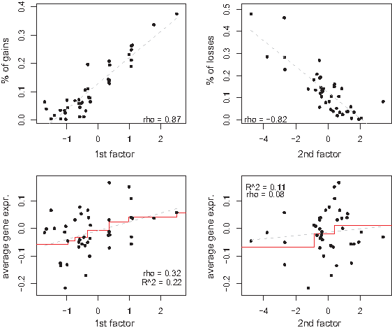
In another example, as shown in the upper panels of Figure 4, the first factor is associated with the percentage of gains whereas the second factor with the percentage of losses. Globally we expect both factors of this GO node to have an effect on the pathway's average gene expression, as is confirmed by GlobalANCOVA (p-value, Factor 1: 1.62 × 10⁻⁷²; p-value, Factor 2: 5.27 × 10⁻¹²). In fact, both should have a positive effect as an increase of the number of gains as well as a decrease in the number of losses are expected to lead to a surge in transcription levels. The lower panels of Figure 4 confirm this for the first factor, but show only a weak positive correlation for the second. Indeed, a multivariate regression analysis returns positive coefficients for both factors, but only finds the first factor to have a significant association with the GO node's gene expression. A more in-depth univariate analysis of the GO node's 91 genes is needed to provide a better understanding of the significance of the second factor as found by GlobalANCOVA.

FIG. 4.

(Left upper panel) First factor versus the percentage of gains. (Right upper panel) Second factor versus the percentage of losses. (Left lower panel) First factor versus average gene expression. (Right lower panel) Second factor versus average gene expression. The gray line in the lower panels is the linear regression line, and the red line is the isotonic regression line.

Others (Ferreira et al., 2008; Järvinen et al., 2008; Lee et al., 2008; Van Wieringen and Van de Wiel, 2009) have also studied copy number and gene expression data jointly within pathways. The analyses in these articles all boil down to a univariate analysis (which genes show an association between copy number and gene expression levels), followed by a gene set enrichment procedure (Subramanian et al., 2005) revealing pathways with an excess of genes with an association between the molecular levels. Although an obvious approach, it ignores much of the complexity of the data. We do not claim to have resolved this complexity with the analysis presented above. But as EFA captures the key characteristics of the pathway copy number data through a multivariate analysis, the key characteristics may be more helpful to explore the complexity of data from the two molecular levels within pathways.

3.4. Comparison

The exploratory factor analysis results of a GO node's call probability data are compared with principal component analysis of the normalized and the segmented array CGH data, as is done by, for example, Somiari et al. (2004) and Unger et al. (2008). To this end, we take the set of 250 GO nodes used previously. For each GO node, we calculate the first principal component (corresponding to the largest eigenvalue) of both the normalized and segmented data. These are used to calculate the Spearman rank correlation coefficient between the principal components and sum of the absolute log₂ ratios of the genes in the GO node. The latter is a proxy for the proportion of aberrations. We also test the association between the components and the GO node's multivariate expression using GlobalANCOVA. These results are compared to the results of the analyses in Sections 3.1 and 3.3. Figure S5 in the Supplementary Material displays the comparison between the results of EFA and PCA on the segmented data.

The figure shows that the factors constructed with the EFA tend to be higher correlated with the proportion of aberrations than the principal components of the segmented data. The figure also reveals that the factors are more significantly associated with the gene expression than these principal components. PCA of normalized array CGH performed worse than both EFA and PCA with segmented data (results not shown). Overall we conclude that EFA is to be preferred over the PCA of either normalized or segmented data.

Besides these quantitative arguments, there is also an important qualitative argument in favor of EFA. Exploratory statistical techniques like EFA and PCA aim to identify salient features of the data. Interpretation of the identified salient features may lead to the generation of new hypotheses regarding the phenomenon under study. It is this interpretation that EFA factors naturally inherit from the call probabilities, and which facilitates understanding and hypothesis generation. The interpretation of the PCA principal components is much harder, see for instance our use of a proxy for the proportion of aberrations in the quantitative comparison above.

4. Conclusion

We presented EFA to characterize the variability in a pathway's copy number data. The proposed method introduces latent variables to model this variability and uses an EM algorithm to fit the model. Practical guidelines as how to assign meaning to the latent variables are given. The potential of our exploratory factor analysis was illustrated in two breast cancer data sets, where it identified several salient features of the studied GO nodes' copy number data. Among others the method suggested that the proportion of aberrations is a key characteristic of a pathway's CNA pattern. It also suggested that another key characteristic may be found in gain-vs-loss contrasts, which should possibly be limited to a subset of genes in the pathway. These clear interpretations stem from the fact that EFA analyzes copy number data represented as call probabilities, and are not possible with convential PCA. In the GO nodes studied, the EFA characteristics were often significantly associated with the node's gene expression data, and may be considered to capture the pathway's global effect of copy number changes on transcription levels. In particular, it yields a better association with gene expression (in terms of R² and p-value) than univariately based approaches that have employed to analyze data from the two platforms. Finally, the results of EFA may support results from hierarchical clustering and be useful for low dimensional plotting. In all, we believe that EFA will prove to be a fruitful technique for exploratory analysis of pathway copy number data.

Footnotes

Disclosure Statement

No competing financial interests exist.

References

Aitchison

1992. The statistical analysis of compositional data. J. R. Stat. Soc. Series B Stat. Methodol., 44:139–177.

Alter

, Brown

P.O.

, Botstein

2000. Singular value decomposition for genome-wide expression data processing and modeling. Proc. Natl. Acad. Sci. USA, 97:10101–10106.

Bartholomew

D.J.

, Knott

1999. Latent Variable Models and Factor Analysis. Oxford University Press: New York.

Bergamaschi

, Kim

Y.H.

, Wang

et al. 2006. Distinct patterns of DNA copy number alteration are associated with different clinicopathological features and gene-expression subtypes of breast cancer. Genes Chromosomes Cancer, 45:1033–1040.

Ferreira

B.I.

, Alonso

, Carrillo

et al. 2008. Array CGH and gene-expression profiling reveals distinct genomic instability patterns associated with DNA repair and cell-cycle checkpoint pathways in ewing's sarcoma. Oncogene, 27:2084–2090.

Fisher

R.A.

1932. Statistical Methods for Research Workers, 4th. Oliver and Boyd: London.

Gene Ontology Consortium. 2000. Gene Ontology: tool for the unification of biology. Nat. Genet., 25:25–29.

Gonzalez

J.R.

, Subirana

, Escarams

et al. 2009. Accounting for uncertainty when assessing association between copy number and disease: a latent class model. BMC Bioinformatics, 10:172.

Hanahan

, Weinberg

2000. The hallmarks of cancer. Cell, 100:57–70.

10.

Hummel

, Meister

, Mansmann

2008. GlobalANCOVA: exploration and assessment of gene group effects. Bioinformatics, 24:78–85.

11.

Järvinen

A.-K.

, Autio

, Kilpinen

et al. 2008. High-resolution copy number and gene expression microarray analyses of head and neck squamous cell carcinoma cell lines of tongue and larynx. Genes Chromosomes Cancer, 47:500–509.

12.

Jöreskog

, Moustaki

2001. Factor analysis of ordinal variables: a comparison of three approaches. Multivar. Behav. Res., 36:347–387.

13.

Khatri

, Draghici

2005. Ontological analysis of gene expression data: current tools, limitations, and open problems. Bioinformatics, 21:3587–3595.

14.

Kotz

, Balakrishnana

, Johnson

2000. Continuous Multivariate Distributions, Volume 1: Models and Applications. Wiley: New York.

15.

LaPointe

, Li

, Higgins

J.P.

et al. 2004. Gene expression profiling identifies clinically relevant subtypes of prostate cancer. Proc. Natl. Acad. Sci. USA, 101:811–816.

16.

Lee

, Kong

S.W.

, Park

P.J.

2008. Integrative analysis reveals the direct and indirect interactions between dna copy number aberrations and gene expression changes. Bioinformatics, 24:889–896.

17.

Lengauer

, Kinzler

, Vogelstein

1998. Genetic instabilities in human cancers. Nature, 396:623–627.

18.

McCullagh

, Nelder

J.A.

2000. Generalized Linear Models. Chapman & Hall: New York.

19.

Neuvial

, Hupe

, Brito

et al. 2006. Spatial normalization of array-CGH data. BMC Bioinformatics, 7:264.

20.

Ogata

, Goto

, Sato

et al. 1999. KEGG: Kyoto Encyclopedia of Genes and Genomes. Nucleic Acids Res., 27:29–34.

21.

Olshen

A.B.

, Venkatraman

E.S.

, Lucito

et al. 2004. Circular binary segmentation for the analysis of array-based DNA copy number data. Biostatistics, 5:557–572.

22.

Perou

C.M.

, Sorlie

, Eisen

M.B.

et al. 2000. Molecular portraits of human breast tumours. Nature, 406:747–752.

23.

Pinkel

, Albertson

2005. Array comparative genomic hybridization and its application in cancer. Nat. Genet., 37:S11–S17.

24.

Pollack

J.R.

, Sorlie

, Perou

C.M.

et al. 2002. Microarray analysis reveals a major direct role of DNA copy number alteration in the transcriptional program of human breast tumors. Proc. Natl. Acad. Sci. USA, 99:12963–12968.

25.

, Tan

, Kutner

M.H.

1996. Random effects models in latent class analysis for evaluating accuracy of diagnostic tests. Biometrics, 52:797–810.

26.

Schneeweiss

, Mathes

1995. Factor analysis and principal components. J. Multivar. Anal., 55:105–124.

27.

Somiari

, Shriver

, He

et al. 2004. Global search for chromosomal abnormalities in infiltrating ductal carcinoma of the breast using array-comparative genomic hybridization. Cancer Genet. Cytogenet., 155:108–118.

28.

Subramanian

, Tamayo

, Mootha

V.K.

et al. 2005. Gene set enrichment analysis: a knowledge-based approach for interpreting genome-wide expression profiles. Proc. Natl. Acad. Sci. USA, 102:15545–15550.

29.

Unger

, Malisch

, Thomas

et al. 2008. Array CGH demonstrates characteristic aberration signatures in human papillary thyroid carcinomas governed by RET/PTC. Oncogene, 27:4592–4602.

30.

Valentijn

L.J.

, Koppen

, Van Asperen

et al. 2005. Inhibition of a new differentiation pathway in neuroblastoma by copy number defects of N-myc, Cdc42, and nm23 genes. Cancer Res., 65:3136–3145.

31.

Van de Wiel

M.A.

, Van Wieringen

W.N.

2007. CGHregions: dimension reduction for array CGH data with minimal information loss. Cancer Informatics, 2:55–63.

32.

Van de Wiel

M.A.

, Kim

K.I.

, Vosse

S.J.

et al. 2007. CGHcall: calling aberrations for array CGH tumor profiles. Bioinformatics, 23:892–894.

33.

Van Wieringen

W.N.

, Van de Wiel

M.A.

2009. Nonparametric testing for DNA copy number induced differential mRNA gene expression. Biometrics, 65:19–29.

34.

Van Wieringen

W.N.

, Van de Wiel

M.A.

, Ylstra

2007. Normalized, segmented or called aCGH data? Cancer Informatics, 3:331–337.

35.

Vogelstein

, Kinzler

K.W.

2004. Cancer genes and the pathways they control. Nat. Med., 10:789–799.

Supplementary Material

Please find the following supplemental material available below.

For Open Access articles published under a Creative Commons License, all supplemental material carries the same license as the article it is associated with.

For non-Open Access articles published, all supplemental material carries a non-exclusive license, and permission requests for re-use of supplemental material or any part of supplemental material shall be sent directly to the copyright owner as specified in the copyright notice associated with the article.

0.00 MB

1.02 MB