An Up-Down Bit Pattern Approach to Coregulated and Negative-Coregulated Gene Clustering of Microarray Data

Abstract

Biclustering, which performs simultaneous clustering of rows (e.g., genes) and columns (e.g., conditions), has been shown to be important for analyzing microarray data. To find biclusters, there have been many methods proposed. Most of these methods can find only clusters with coregulated patterns, which means that the expression levels of genes in a found cluster rise and fall simultaneously. However, for real microarray data, there exist negative-correlated patterns, which means that the tendencies of expression levels of some genes may be completely inverse to those of the other genes under some conditions. Although one method called Co-gclustering was proposed to simultaneously find clusters with correlated and negative-correlated patterns, its time complexity is exponential to the number of conditions, which may not be efficient. Therefore, in this article, we propose a new method, Up-Down Bit pattern (UDB), to efficiently find clusters with correlated and negative-correlated patterns. First, we utilize up-down bit patterns to record those condition pairs where one gene is upregulated or downregulated. One gene is upregulated (or downregulated) under condition pair a and b if its expression level shows an upward (or downward) tendency from condition a to condition b. Then, we apply a heuristic idea on these up-down bit patterns to efficiently find clusters, which will reduce the time complexity from exponential time to polynomial time. From the experimental results, we show that the UDB method is more efficient than the Co-gclustering method.

1. Introduction

Microarrays provide a powerful tool in experimental molecular biology by which the expression patterns of thousands of genes can be monitored simultaneously (Yang et al., 2005). The microarray data are usually organized as a matrix, composed of m rows representing m genes and n columns representing n samples (or experimental conditions). The value of each cell in this matrix represents the expression level of one particular gene under one particular condition (Yang et al., 2005). The value of m, usually from 10³ to 10⁴, is much larger than the value of n, usually less than 10². Clustering the microarray data into homogeneous groups was shown to be instrumental in functional annotation, tissue classification, and motif identification (Tanay et al., 2002).

Traditional clustering methods work in the full dimensional space, and can only be applied to either the rows or the columns of a data matrix, separately (Aguilar-Ruiz, 2005; Zhao and Zaki, 2005). However, investigations show that more often than not, several genes contribute to the same pathway, which motivates researchers to identify a subset of genes whose expression levels rise and fall coherently under a subset of conditions (Yang et al., 2005). Moreover, for traditional clustering methods, one object (i.e., one gene) is commonly assigned to one cluster. In fact, genes may participate in several biological functions and thus should be included in multiple clusters (Ihmels et al., 2004). Therefore, biclustering (Cheng and Church, 2000) was proposed, which does not have those limitations. Biclustering performs simultaneous clustering of rows and columns. If some objects (genes) are similar under some conditions (i.e., a subspace), they will be clustered together in that subspace. Biclustering has proved of great value for finding interesting patterns from microarray data (Zhao and Zaki, 2005).

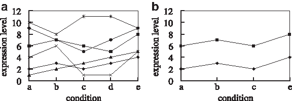
There have been several types of biclusters proposed (Madeira and Oliveira, 2004). Among these types, biclusters with coherent values define a bicluster as a subset of genes and a subset of conditions of the microarray data which have coherent values of expression levels on both rows and columns (Madeira and Oliveira, 2004). Figure 1 shows an example, where Figure 1a shows the expression patterns of 6 genes of one microarray data matrix on the full space, i.e., all conditions, and Figure 1b shows a bicluster of 2 genes with coherent values on only the subspace, i.e., conditions a, b, c, and e. Methods for biclusters with coherent values (Chang et al., 2009; Cheng and Church, 2000; Wang et al., 2002; Yoon et al., 2005; Zhao and Zaki, 2005) aim to cluster those genes whose expression values have simple linear transformation relationships. Genes in such a bicluster have been shown to have significant biological relationships among these genes (Zhao and Zaki, 2005). However, the definition of biclusters with coherent values is sometimes too strict, since it only allows a simple linear transformation among the expression values of genes. For some microarray data matrices, it may be very difficult to find such a bicluster. Another type of biclusters, biclusters with coherent evolutions, does not have such a limitation. This type of biclusters aims to find a subset of genes up-regulated or down-regulated across a subset of conditions without taking into account their actual expression values (Madeira and Oliveira, 2004). Figure 2 shows an example of one bicluster of 3 genes with coherent evolutions for the expression data shown in Figure 1a.

FIG. 1.

An example of biclustering. (a) The expression patterns of six genes on the full space. (b) A bicluster of two genes with coherent values.

FIG. 2.

A bicluster of three genes with coherent evolutions.

In Zhao et al. (2008), they further considered the negative-correlated pattern. That is, the tendencies of expression values of some genes are completely inverse to those of the other genes. Figure 3 shows an example of the negative-correlated pattern for the expression data shown in Figure 1a, where the top gene shows an inverse tendency of expression values against the other three genes. There have been many genes proved to have such behavior. For example, for genes of the yeast, genes YLR367W and YKR057W share the same tendency, while they have a negative-correlated pattern against gene YML009C under 8 conditions (Zhao et al., 2008). It has been suggested that all these genes are involved in protein translation and translocation and should be grouped into the same cluster (Breitkreutz et al., 2006; Zhao et al., 2008). In this article, we will focus on the design of an efficient method for finding biclusters containing both correlated and negative-correlated patterns.

FIG. 3.

A bicluster of four genes containing both correlated and negative-correlated patterns.

According to the definition of a up/down regulation, methods of finding biclusters with coherent evolutions could be classified into two types: one focusing on the expression value of one gene under each single condition, and the other one focusing on the variation of expression values of one gene from one condition to another condition. For methods of the first type, e.g., SAMBA (Tanay et al., 2002) and BiModule (Okada et al., 2007), they usually define that one gene is up/down-regulated under one single condition if its expression level after standardizing with the mean (e.g., 0) and the variance (e.g., 1) is above/below a certain value (e.g., 1/−1) (Tanay et al., 2002). These methods aim to cluster those genes whose expression levels are commonly up/down-regulated under some conditions. However, they do not consider the relationship between expression levels of two conditions for one gene, which may not be precise enough occasionally. For example, these methods may find that both genes 1 and 2 are upregulated under both condition a and condition b. However, the expression levels of gene 1 from condition a to condition b may be increasing, while the expression levels of gene 2 from condition a to condition b may be decreasing. For methods of the second type, e.g., OPSM (Ben-Dor et al., 2003), OP-Cluster (Liu and Wang, 2003), and Co-gclustering (Zhao et al., 2008), they take into consideration the variation of expression values of one gene from one condition to another condition. In Ben-Dor et al. (2003), a submatrix of the expression data is an OPSM cluster if there is a permutation of its columns under which the sequence of values in every row is strictly increasing. The OP-Cluster method (Liu and Wang, 2003) also tries to find the OPSM clusters by transforming this problem into a sequential pattern mining-like problem. These methods consider the numeral order of expression levels between every two conditions, and aim to cluster those genes whose expression levels are increasing under one permutation of conditions. Although all the above methods may efficiently find clusters with correlated patterns, they can not find clusters with negative-correlated patterns. Therefore, the Co-gclustering method (Zhao et al., 2008) was proposed. This method utilizes a tree structure to gradually generate all the answers, and can simultaneously find clusters with correlated and negative-correlated patterns.

Although the Co-gclustering method can find clusters with correlated and negative-correlated patterns, the tree constructing process of this method may not be efficient. Assuming that the number of conditions is n, in the worst case, this method needs to generate (n − 1) trees, where each tree represents one combination of k conditions for 2 ≤ k ≤ n. The time complexity of this method is O(2ⁿ). Even though the Co-gclustering method utilizes a technique which reduces the number of trees being generated, for real microarray data, the effect of this technique is still limited and could not significantly reduce its time complexity.

Therefore, in this article, we propose a new method, Up-Down Bit pattern (UDB), to efficiently find clusters with correlated and negative-correlated patterns. In the UDB method, first, we utilize up-down bit patterns to record those condition pairs where one gene is upregulated or downregulated. One gene is upregulated (or downregulated) under condition pair a and b if its expression level shows an upward (or downward) tendency from condition a to condition b. For each gene, its up bit pattern and down bit pattern are two bit strings with length \documentclass{aastex} \usepackage{amsbsy} \usepackage{amsfonts} \usepackage{amssymb} \usepackage{bm} \usepackage{mathrsfs} \usepackage{pifont} \usepackage{stmaryrd} \usepackage{textcomp} \usepackage{portland, xspace} \usepackage{amsmath, amsxtra} \pagestyle{empty} \DeclareMathSizes {10} {9} {7} {6} \begin{document} $${\rm C}^n_2$$ \end{document} , respectively, where each bit corresponds to one condition pair. One bit of the up (or down) bit pattern of one gene is set to 1, if this gene is significantly upregulated (or downregulated) under the condition pair corresponding to that bit. Then, we apply a heuristic idea on these up-down bit patterns to efficiently find clusters. The idea is that for every two genes, we directly utilize two rules to determine whether they should be in the same cluster. These two rules apply bit operations on the up-down bit patterns of two genes, to check whether these two genes are coregulated or negative-coregulated under an enough number of condition pairs. The time complexity of this step is O(m²), where m is the number of genes. As compared to the Co-gclustering method, we reduce the time complexity from exponential time (i.e., O(2ⁿ), where n is the number of conditions) to polynomial time (i.e., O(m²)). Our cost for this reduction is that some genes in one found cluster may not be completely similar to each other according to our definition of similarity. Therefore, we further propose post-processes for processing those found clusters to redeem this problem. From the experimental results on several synthetic and real microarray data sets, we show that the UDB method is more efficient than the Co-gclustering method. Moreover, we will show the correlation of genes in clusters found by the UDB method for real microarray data.

The rest of this article is organized as follows. In Section 2, we give a survey of the Co-gclustering method. Section 3 presents the proposed UDB method. In Section 4, we study the performance of the UDB method and make a comparison with the Co-gclustering method. Finally, we make a conclusion in Section 5.

2. Related Work

In this section, we introduce the Co-gclustering method (Zhao et al., 2008). In 2008, Zhao et al. proposed the Co-gclustering method to find biclusters containing both correlated and negative-correlated patterns. Given a microarray data matrix with m genes and n conditions, for each gene g_i, this method first finds all significant p-pairs (prototypal sequence pairs), (c_j, c_k). Assume that the expression levels of gene g_i under condition c_j and c_k are d_i,j and d_i,k, respectively. A significant p-pair can be either upregulated when \documentclass{aastex} \usepackage{amsbsy} \usepackage{amsfonts} \usepackage{amssymb} \usepackage{bm} \usepackage{mathrsfs} \usepackage{pifont} \usepackage{stmaryrd} \usepackage{textcomp} \usepackage{portland, xspace} \usepackage{amsmath, amsxtra} \pagestyle{empty} \DeclareMathSizes {10} {9} {7} {6} \begin{document} $$d_{i , k} - d_{i , j} > \epsilon \times \mid d_{i , j} \mid$$ \end{document} , or downregulated when \documentclass{aastex} \usepackage{amsbsy} \usepackage{amsfonts} \usepackage{amssymb} \usepackage{bm} \usepackage{mathrsfs} \usepackage{pifont} \usepackage{stmaryrd} \usepackage{textcomp} \usepackage{portland, xspace} \usepackage{amsmath, amsxtra} \pagestyle{empty} \DeclareMathSizes {10} {9} {7} {6} \begin{document} $$d_{i , k} - d_{i , j} < - \epsilon \times \mid d_{i , j} \mid$$ \end{document} , where \documentclass{aastex} \usepackage{amsbsy} \usepackage{amsfonts} \usepackage{amssymb} \usepackage{bm} \usepackage{mathrsfs} \usepackage{pifont} \usepackage{stmaryrd} \usepackage{textcomp} \usepackage{portland, xspace} \usepackage{amsmath, amsxtra} \pagestyle{empty} \DeclareMathSizes {10} {9} {7} {6} \begin{document} $$\epsilon$$ \end{document} is the regulation threshold. The information of all the significant p-pairs for each gene are stored in a regulation significance table. Next, this method constructs a Co-tree with height 1, T₁, from the regulation significance table. Co-tree T₁ is a tree with three levels, where nodes of the first and the second levels are for storing the conditions of p-pairs, and nodes of the third level (i.e., leaf nodes) are for storing the genes of p-pairs. Genes stored in the leaf nodes are further classified into two clusters: the ↗-cluster for genes from upregulated p-pairs, and the ↘-cluster for genes from downregulated p-pairs.

Then, this method constructs Co-tree T₂ from T₁. Two p-pairs (c_i, c_j) and (c_j, c_k) in T₁ are concatenated to form a new 2-segment ((c_i, c_j), (c_j, c_k)) in T₂, where this 2-segment represents a path from the root node to the leaf node, i.e., (c_i, c_j, c_k), of T₂. For genes stored in the leaf nodes, they are also divided into two clusters, the S-cluster and the D-cluster. The S-cluster for segment ((c_i, c_j), (c_j, c_k)) is the union of all genes in (the ↗-cluster of (c_i, c_j) ∩ the ↗-cluster of (c_j, c_k)) and (the ↘-cluster of (c_i, c_j) ∩ the ↘-cluster of (c_j, c_k)). The D-cluster for segment ((c_i, c_j), (c_j, c_k)) is the union of all genes in (the ↗-cluster of (c_i, c_j) ∩ the ↘-cluster of (c_j, c_k)) and (the ↘-cluster of (c_i, c_j) ∩ the ↗-cluster of (c_j, c_k)). For genes in the same cluster, this method further utilizes a dissimilarity threshold, δ, to verify the similarity of every two genes. If two genes can not satisfy this threshold, they are divided into two different clusters. After checking the dissimilarity threshold, this method also checks whether the number of genes of each cluster is not less than α, where α is the parameter of the minimal number of genes of a found cluster. Genes in the same cluster form a Co-gcluster if the number of conditions along the path from the root node to the leaf node is not less than β, where β is the parameter of the minimal number of conditions of a found cluster.

For the rest of Co-trees, T_l where l ≥ 3, they are constructed from those previous Co-trees. Two segments of a Co-tree can be concatenated together to form a new path in the new Co-tree, if the last p-pair of the former segment is the same as the first p-pair of the later segment. This technique is called β-jumping in the Co-gclustering method. For example, for two 3-segments of T₃, ((c₁, c₂), (c₂, c₃), (c₃, c₄)) and ((c₃, c₄), (c₄, c₅), (c₅, c₆)), they can be concatenated together to form a new 5-segment ((c₁, c₂), (c₂, c₃), (c₃, c₄), (c₄, c₅), (c₅, c₆)) in T₅. The S-cluster for this new 5-segment is the union of all genes in (the S-cluster of ((c₁, c₂), (c₂, c₃), (c₃, c₄)) ∩ the S-cluster of ((c₃, c₄), (c₄, c₅), (c₅, c₆)) and (the D-cluster of ((c₁, c₂), (c₂, c₃), (c₃, c₄)) ∩ the D-cluster of ((c₃, c₄), (c₄, c₅), (c₅, c₆)). The D-cluster for this new 5-segment is the union of all genes in (the S-cluster of ((c₁, c₂), (c₂, c₃), (c₃, c₄)) ∩ the D-cluster of ((c₃, c₄), (c₄, c₅), (c₅, c₆)) and (the D-cluster of ((c₁, c₂), (c₂, c₃), (c₃, c₄)) ∩ the S-cluster of ((c₃, c₄), (c₄, c₅), (c₅, c₆)). This technique can be applied until T_β₋₁. For those Co-trees T_l where l ≥ β, they need to be constructed gradually from T_l₋₁.

The Co-gclustering method utilizes the β-jumping technique to avoid generating all Co-trees T_l for l ≤ n. However, for real microarray data, we have no knowledge about the possible number of conditions of a found cluster. For the Co-gclustering method, if parameter β is set to a large value close to the maximal possible number of conditions of found clusters, there may exist some interesting clusters being dropped due to this large value of β. If parameter β is set to a value much less than the maximal possible number of conditions of found clusters, this method needs to construct all Co-trees T_l for l ≥ β. The time complexity in the worst case is O(2ⁿ), i.e., enumerating the power set of n conditions. Therefore, this tree constructing process may not be efficient.

3. Proposed Method

In this section, we present our method, Up-Down Bit pattern (UDB), for finding clusters which contain both coregulated and negative-coregulated patterns in microarray data. Table 1 shows the variables used in the UDB method, and Figure 4 shows the UDB method. The UDB method has three main steps: (1) determining up-down bit patterns of each gene, (2) clustering those genes which share the same tendency based on up-down bit patterns, and (3) post-processing the found clusters. We will describe these steps in the following subsections.

FIG. 4.

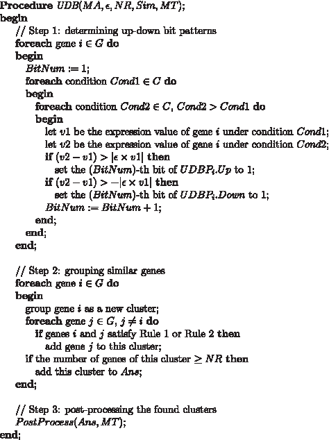
The UDB method.

Table 1.

Variables Used in the Proposed Method

Variable	Description
MA	A two-dimensional gene expression matrix
G	The set of genes of MA
C	The set of conditions of MA
\documentclass{aastex} \usepackage{amsbsy} \usepackage{amsfonts} \usepackage{amssymb} \usepackage{bm} \usepackage{mathrsfs} \usepackage{pifont} \usepackage{stmaryrd} \usepackage{textcomp} \usepackage{portland, xspace} \usepackage{amsmath, amsxtra} \pagestyle{empty} \DeclareMathSizes {10} {9} {7} {6} \begin{document} $$\epsilon$$ \end{document}	The threshold for defining up/down-regulation
NR	The minimal number of genes (rows) of a cluster
Sim	The threshold for defining the similarity of a cluster
UDBP_i	The up-down bit patterns of gene i, containing two fields:
	(1) Up, a bit string which indicates those condition pairs where gene i is upregulated, and
	(2) Down, a bit string which indicates those condition pairs where gene i is downregulated
Clust	A coregulated cluster, containing two fields:
	(1) GeneSet, a set of coregulated genes, and
	(2) CondBit, a bit string which indicates the related conditions
Ans	The set of coregulated clusters in MA
MT	The merging threshold

3.1. Step 1

In Step 1, we determine the up-down bit patterns for each gene. For each gene, we compute the difference of expression values of this gene under every two conditions (denoted as Cond1 and Cond2). If this difference is positive, it means that the gene is upregulated (i.e., an upward tendency) from condition Cond1 to condition Cond2. If this difference is negative, it means that the gene is downregulated (i.e., a downward tendency) from condition Cond1 to condition Cond2.

Formally, the same as the definition in Zhao et al. (2008), we also have a threshold, \documentclass{aastex} \usepackage{amsbsy} \usepackage{amsfonts} \usepackage{amssymb} \usepackage{bm} \usepackage{mathrsfs} \usepackage{pifont} \usepackage{stmaryrd} \usepackage{textcomp} \usepackage{portland, xspace} \usepackage{amsmath, amsxtra} \pagestyle{empty} \DeclareMathSizes {10} {9} {7} {6} \begin{document} $$\epsilon$$ \end{document} , for defining significant up/down-regulation, where \documentclass{aastex} \usepackage{amsbsy} \usepackage{amsfonts} \usepackage{amssymb} \usepackage{bm} \usepackage{mathrsfs} \usepackage{pifont} \usepackage{stmaryrd} \usepackage{textcomp} \usepackage{portland, xspace} \usepackage{amsmath, amsxtra} \pagestyle{empty} \DeclareMathSizes {10} {9} {7} {6} \begin{document} $$\epsilon \geq 0$$ \end{document} . Assume that for gene i, its expression values under conditions Cond1 and Cond2 are v1 and v2, respectively. Then, gene i is significantly upregulated from condition Cond1 to condition Cond2, if \documentclass{aastex} \usepackage{amsbsy} \usepackage{amsfonts} \usepackage{amssymb} \usepackage{bm} \usepackage{mathrsfs} \usepackage{pifont} \usepackage{stmaryrd} \usepackage{textcomp} \usepackage{portland, xspace} \usepackage{amsmath, amsxtra} \pagestyle{empty} \DeclareMathSizes {10} {9} {7} {6} \begin{document} $$(v2 - v1) > \mid \epsilon \times v1 \mid$$ \end{document} . This means that the growth rate of expression values of gene i from condition Cond1 to condition Cond2 is above \documentclass{aastex} \usepackage{amsbsy} \usepackage{amsfonts} \usepackage{amssymb} \usepackage{bm} \usepackage{mathrsfs} \usepackage{pifont} \usepackage{stmaryrd} \usepackage{textcomp} \usepackage{portland, xspace} \usepackage{amsmath, amsxtra} \pagestyle{empty} \DeclareMathSizes {10} {9} {7} {6} \begin{document} $$(\epsilon \times 100)$$ \end{document} percent. Similarly, gene i is significantly downregulated from condition Cond1 to Cond2, if \documentclass{aastex} \usepackage{amsbsy} \usepackage{amsfonts} \usepackage{amssymb} \usepackage{bm} \usepackage{mathrsfs} \usepackage{pifont} \usepackage{stmaryrd} \usepackage{textcomp} \usepackage{portland, xspace} \usepackage{amsmath, amsxtra} \pagestyle{empty} \DeclareMathSizes {10} {9} {7} {6} \begin{document} $$(v2 - v1) < - \mid \epsilon \times v1 \mid$$ \end{document} . This means that the reduction rate of expression values of gene i from condition Cond1 to condition Cond2 is above \documentclass{aastex} \usepackage{amsbsy} \usepackage{amsfonts} \usepackage{amssymb} \usepackage{bm} \usepackage{mathrsfs} \usepackage{pifont} \usepackage{stmaryrd} \usepackage{textcomp} \usepackage{portland, xspace} \usepackage{amsmath, amsxtra} \pagestyle{empty} \DeclareMathSizes {10} {9} {7} {6} \begin{document} $$(\epsilon \times 100)$$ \end{document} percent. Take the gene expression matrix shown in Figure 5 as an example. Assume \documentclass{aastex} \usepackage{amsbsy} \usepackage{amsfonts} \usepackage{amssymb} \usepackage{bm} \usepackage{mathrsfs} \usepackage{pifont} \usepackage{stmaryrd} \usepackage{textcomp} \usepackage{portland, xspace} \usepackage{amsmath, amsxtra} \pagestyle{empty} \DeclareMathSizes {10} {9} {7} {6} \begin{document} $$\epsilon = 0.01$$ \end{document} . Gene 1 is significantly upregulated from condition a to condition b, since \documentclass{aastex} \usepackage{amsbsy} \usepackage{amsfonts} \usepackage{amssymb} \usepackage{bm} \usepackage{mathrsfs} \usepackage{pifont} \usepackage{stmaryrd} \usepackage{textcomp} \usepackage{portland, xspace} \usepackage{amsmath, amsxtra} \pagestyle{empty} \DeclareMathSizes {10} {9} {7} {6} \begin{document} $$(v2 - v1) = (3 - 1) > \mid \epsilon \times v1 \mid = \mid 0.01 \times 1 \mid$$ \end{document} . Gene 1 is significantly downregulated from condition b to condition c, since \documentclass{aastex} \usepackage{amsbsy} \usepackage{amsfonts} \usepackage{amssymb} \usepackage{bm} \usepackage{mathrsfs} \usepackage{pifont} \usepackage{stmaryrd} \usepackage{textcomp} \usepackage{portland, xspace} \usepackage{amsmath, amsxtra} \pagestyle{empty} \DeclareMathSizes {10} {9} {7} {6} \begin{document} $$(v2 - v1) = (2 - 3) < - \mid \epsilon \times v1 \mid = - \mid 0.01 \times 3 \mid$$ \end{document} .

FIG. 5.

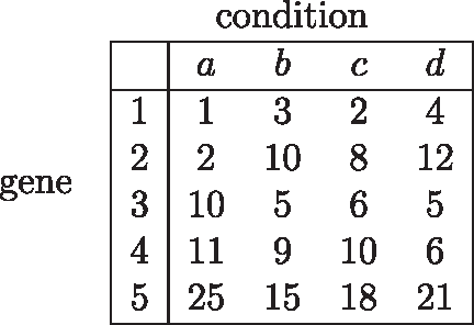
An example gene expression matrix.

We utilize up-down bit patterns to record the condition pairs where gene i is upregulated or downregulated. The up and down bit patterns of gene i are denoted as UDBP_i.Up and UDBP_i.Down, respectively. UDBP_i.Up and UDBP_i.Down are initially two bit strings with all bits equal to 0. One bit of UDBP_i.Up (or UDBP_i.Down) is set to 1, if gene i is significantly upregulated (or downregulated) under the condition pair corresponding to that bit. As shown in Step 1 of Figure 4, we use an increasing number, BitNum, to record the corresponding bit number for condition pair Cond1 and Cond2. The value of BitNum is one-to-one mapping to one combination of Cond1 and Cond2. Assume that the number of total conditions is n. The lengths of UDBP_i.Up and UDBP_i.Down are both \documentclass{aastex} \usepackage{amsbsy} \usepackage{amsfonts} \usepackage{amssymb} \usepackage{bm} \usepackage{mathrsfs} \usepackage{pifont} \usepackage{stmaryrd} \usepackage{textcomp} \usepackage{portland, xspace} \usepackage{amsmath, amsxtra} \pagestyle{empty} \DeclareMathSizes {10} {9} {7} {6} \begin{document} $$C^n_2$$ \end{document} , and \documentclass{aastex} \usepackage{amsbsy} \usepackage{amsfonts} \usepackage{amssymb} \usepackage{bm} \usepackage{mathrsfs} \usepackage{pifont} \usepackage{stmaryrd} \usepackage{textcomp} \usepackage{portland, xspace} \usepackage{amsmath, amsxtra} \pagestyle{empty} \DeclareMathSizes {10} {9} {7} {6} \begin{document} $$1 \leq BitNum \leq C^n_2$$ \end{document} .

Figure 6 shows the up-down bit patterns for the example shown in Figure 5, where Figure 6a shows the differences of expression values between each condition pair, and Figure 6b shows the up-down bit patterns of each gene. The value of \documentclass{aastex} \usepackage{amsbsy} \usepackage{amsfonts} \usepackage{amssymb} \usepackage{bm} \usepackage{mathrsfs} \usepackage{pifont} \usepackage{stmaryrd} \usepackage{textcomp} \usepackage{portland, xspace} \usepackage{amsmath, amsxtra} \pagestyle{empty} \DeclareMathSizes {10} {9} {7} {6} \begin{document} $$\epsilon$$ \end{document} is 0.01. For gene 1, we first consider the difference of expression values from condition a to condition b, i.e., (b − a). The corresponding bit for (b − a) in our up-down bit patterns is bit (BitNum = 1) (denoted as “a → b” in Figure 6b). Since this difference value is 2 > |0.01 × 1|, we set bit 1 ( = BitNum) of the up bit pattern of gene 1, i.e., UDBP₁.Up, to 1. The value of BitNum is then increased by 1. Next, we consider the difference value of (c − a). The corresponding bit for (c − a) is therefore bit (BitNum = 2). Since this difference value is 1 > |0.01 × 1|, we set bit 2 of UDBP₁.Up to 1. The value of BitNum is increased by 1 again. Bit 3 of UDBP₁.Up, corresponding to (d − a), is also set to 1 in the same way. The value of BitNum becomes 4 now. For the difference value of (c − b), i.e., −1, it is not larger than \documentclass{aastex} \usepackage{amsbsy} \usepackage{amsfonts} \usepackage{amssymb} \usepackage{bm} \usepackage{mathrsfs} \usepackage{pifont} \usepackage{stmaryrd} \usepackage{textcomp} \usepackage{portland, xspace} \usepackage{amsmath, amsxtra} \pagestyle{empty} \DeclareMathSizes {10} {9} {7} {6} \begin{document} $$\mid \epsilon \times 3 \mid = 0.03$$ \end{document} . Therefore, we do not change any bit of UDBP₁.Up. However, since \documentclass{aastex} \usepackage{amsbsy} \usepackage{amsfonts} \usepackage{amssymb} \usepackage{bm} \usepackage{mathrsfs} \usepackage{pifont} \usepackage{stmaryrd} \usepackage{textcomp} \usepackage{portland, xspace} \usepackage{amsmath, amsxtra} \pagestyle{empty} \DeclareMathSizes {10} {9} {7} {6} \begin{document} $$- 1 < - \mid \epsilon \times 3 \mid = - 0.03$$ \end{document} , we set bit 4 ( = BitNum) of UDBP₁.Down to 1. By using the similar idea, we can evaluate the up and down bit patterns of each gene, as shown in Figure 6b.

FIG. 6.

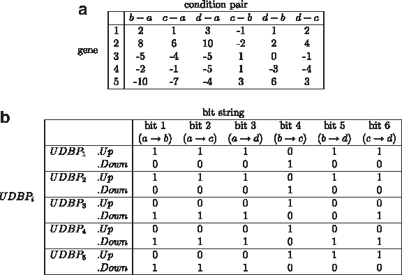
Evaluation of up-down bit patterns: (a) the differences of expression values between each condition pair; (b) the up-down bit patterns of each gene.

3.2. Step 2

In this step, we cluster the similar genes according to their up-down bit patterns determined in Step 1. As shown in Step 2 of Figure 4, for each gene i, we first group it as a new cluster. Then, for each of the rest of genes except gene i, denoted as gene j, it is similar to gene i, if it satisfies the following Rule 1 or Rule 2, where “|one bit string|” means the number of on-bits (“1”) in this bit string:

Rule 1. \documentclass{aastex} \usepackage{amsbsy} \usepackage{amsfonts} \usepackage{amssymb} \usepackage{bm} \usepackage{mathrsfs} \usepackage{pifont} \usepackage{stmaryrd} \usepackage{textcomp} \usepackage{portland, xspace} \usepackage{amsmath, amsxtra} \pagestyle{empty} \DeclareMathSizes {10} {9} {7} {6} \begin{document} $$(\mid UDBP_i.{\underline{Up}} \ \hbox{AND} \ UDBP_j.{\underline{Up}} \mid + \mid UDBP_i.{\underline{Down}} \ \hbox{AND} \ UDBP_j.{\underline{Down}} \mid) \geq Sim \times \hbox{C}^n_2$$ \end{document}

Rule 2. \documentclass{aastex} \usepackage{amsbsy} \usepackage{amsfonts} \usepackage{amssymb} \usepackage{bm} \usepackage{mathrsfs} \usepackage{pifont} \usepackage{stmaryrd} \usepackage{textcomp} \usepackage{portland, xspace} \usepackage{amsmath, amsxtra} \pagestyle{empty} \DeclareMathSizes {10} {9} {7} {6} \begin{document} $$(\mid UDBP_i.{\underline{Up}} \ \hbox{AND} \ UDBP_j.{\underline{Down}} \mid + \mid UDBP_i.{\underline{Down}} \ \hbox{AND} \ UDBP_j.{\underline{Up}} \mid) \geq Sim \times \hbox{C}^n_2$$ \end{document}

In this case, we add gene j to the cluster of gene i.

For Rule 1, the term “UDBP_i.Up AND UDBP_j.Up” means those bits of condition pairs where gene i and gene j are both upregulated. The term “UDBP_i.Down AND UDBP_j.Down” means those bits of condition pairs where gene i and gene j are both downregulated. Therefore, the sum of numbers of on-bits in the above two terms means the number of condition pairs where gene i and gene j are simultaneously upregulated or downregulated. The total number of condition pairs (i.e., the length of each bit string) is \documentclass{aastex} \usepackage{amsbsy} \usepackage{amsfonts} \usepackage{amssymb} \usepackage{bm} \usepackage{mathrsfs} \usepackage{pifont} \usepackage{stmaryrd} \usepackage{textcomp} \usepackage{portland, xspace} \usepackage{amsmath, amsxtra} \pagestyle{empty} \DeclareMathSizes {10} {9} {7} {6} \begin{document} $${\rm C}^n_2$$ \end{document} . Therefore, the closer the sum is to \documentclass{aastex} \usepackage{amsbsy} \usepackage{amsfonts} \usepackage{amssymb} \usepackage{bm} \usepackage{mathrsfs} \usepackage{pifont} \usepackage{stmaryrd} \usepackage{textcomp} \usepackage{portland, xspace} \usepackage{amsmath, amsxtra} \pagestyle{empty} \DeclareMathSizes {10} {9} {7} {6} \begin{document} $${\rm C}^n_2$$ \end{document} , the similar these two genes are to each other. (Note that when these two genes are simultaneously upregulated or downregulated under all condition pairs, this sum will be \documentclass{aastex} \usepackage{amsbsy} \usepackage{amsfonts} \usepackage{amssymb} \usepackage{bm} \usepackage{mathrsfs} \usepackage{pifont} \usepackage{stmaryrd} \usepackage{textcomp} \usepackage{portland, xspace} \usepackage{amsmath, amsxtra} \pagestyle{empty} \DeclareMathSizes {10} {9} {7} {6} \begin{document} $${\rm C}^n_2$$ \end{document} .) Based on this idea, the user can specify parameter Sim to define the similarity of genes in a cluster, where 0 < Sim ≤ 1. For example, for genes 1 and 2 in the previous example shown in Figure 5, their up-down bit patterns are shown in Figure 6b. Assume Sim = 0.9. Then, we have \documentclass{aastex} \usepackage{amsbsy} \usepackage{amsfonts} \usepackage{amssymb} \usepackage{bm} \usepackage{mathrsfs} \usepackage{pifont} \usepackage{stmaryrd} \usepackage{textcomp} \usepackage{portland, xspace} \usepackage{amsmath, amsxtra} \pagestyle{empty} \DeclareMathSizes {10} {9} {7} {6} \begin{document} $$\mid UDBP_1.{\underline{Up}} \ \hbox{AND} \ UDBP_2.{\underline{Up}} \mid + \mid UDBP_1.{\underline{Down}} \ \hbox{AND} \ UDBP_2.{\underline{Down}} \mid = \mid 111011 \mid + \mid 000100 \mid = 6 \geq Sim \times {\rm C}^n_2 = 0.9 \times 6$$ \end{document} . This means that gene 1 and gene 2 are simultaneously coregulated under more than (Sim × 100 = 90) percent of condition pairs. Therefore, gene 2 is similar to gene 1 and is added to the same cluster of gene 1.

Similarly, for Rule 2, it considers the negative-coregulation. That is, when gene i is upregulated (or downregulated), gene j will be downregulated (or upregulated). Therefore, we consider “UDBP_i.Up AND UDBP_j.Down” and “UDBP_i.Down AND UDBP_j.Up”. The sum of numbers of on-bits in the result indicates the number of condition pairs where gene i and gene j show the negative-coregulation. Take the up-down bit patterns of genes 1 and 4 shown in Figure 6b as an example. Assume Sim = 0.9. For these two genes, we have \documentclass{aastex} \usepackage{amsbsy} \usepackage{amsfonts} \usepackage{amssymb} \usepackage{bm} \usepackage{mathrsfs} \usepackage{pifont} \usepackage{stmaryrd} \usepackage{textcomp} \usepackage{portland, xspace} \usepackage{amsmath, amsxtra} \pagestyle{empty} \DeclareMathSizes {10} {9} {7} {6} \begin{document} $$\mid UDBP_1.{\underline{Up}} \ \hbox{AND} \ UDBP_4.{\underline{Down}} \mid + \mid UDBP_1.{\underline{Down}} \ \hbox{AND} \ UDBP_4.{\underline{Up}} \mid = \mid 111011 \mid + \mid 000100 \mid = 6 \geq Sim \times {\rm C}^n_2 = 0.9 \times 6$$ \end{document} . Therefore, gene 4 is also added to the cluster of gene 1.

In Step 2 of Figure 4, based on gene i, all the other genes except gene i will be checked whether they can be added into the cluster of gene i. Then, we check the number of genes within this cluster. Only if this number is above a user specified parameter, NR, this cluster is added into the result set of clustering, Ans. With the similar process, we continue to try to generate a new cluster for the next gene i in G until all genes in G are processed.

Biclustering is originally a NP-Complete problem (Aguilar-Ruiz, 2005; Yang et al., 2005; Yoon et al., 2005; Zhao and Zaki, 2005). Therefore, in the worst case, the time complexity of biclustering methods (Zhao et al., 2008) is O(2ⁿ), where n is the number of conditions. In Step 2 of the proposed UDB method, instead of enumerating the power set of n conditions (which is often used in those previous methods), we utilize a heuristic idea, i.e., two loops with time complexity O(m²), to speed up the process of finding clusters, where m is the number of genes. The benefit is that we reduce the time complexity from exponential time to polynomial time. Our pay is that not every two genes in a found cluster will satisfy the similarity threshold, Sim. For example, assume that we have three genes, e.g., genes 1, 2, and 3. The up bit patterns for genes 1, 2, and 3 are “11111,” “11110,” and “01111,” respectively. The down bit patterns for these genes are all “00000.” If the similarity threshold, Sim, is 0.8, the correct clusters should be {gene 1, gene 2} and {gene 1, gene 3}. In our Step 2, gene 2 and gene 3 will be added into the cluster of gene 1, since “|11111 AND 11110| = 4 ≥ 0.8 × 5” and “|11111 AND 01111| = 4 ≥ 0.8 × 5.” Next, gene 1 is added into the cluster of gene 2. Then, gene 1 is added into the cluster of gene 3. Finally, we find three clusters, {gene 1, gene 2, gene 3}, {gene 1, gene 2}, and {gene 1, gene 3}. The second and the third clusters are the same as the correct ones. Genes in the first cluster do not all satisfy the similarity threshold, since gene 2 (where UDBP₂.Up = “11110”) and gene 3 (where UDBP₃.Up = “01111”) are not similar to each other based on Sim = 0.8. To redeem this problem, we will post-process the found clusters in Step 3 later.

3.3. An improved version of Step 2

For Step 2 described in the previous subsection, we do not record the condition pairs of one cluster where genes in this cluster are coregulated or negative-coregulated under these condition pairs. In this subsection, we present an improved version, Step 2^*, which records the condition pairs.

Figure 7 shows the new process of Step 2^*. The basic idea of Step 2^* is the same as that of Step 2, which also utilizes two loops with time complexity O(m²). One difference is that for each cluster, Clust, it contains the following two fields: (1) GeneSet, a set for storing the genes, and (2) CondBit, a bit string for indicating those condition pairs where genes in GeneSet are coregulated or negative-coregulated. Another difference is that we use two bit strings, UpBit and DownBit, to help us derive CondBit of one cluster. UpBit and DownBit are used to record those condition pairs where genes in this cluster are upregulated and downregulated, respectively. Note that one bit can keep to be “1” after AND operations only if this bit is “1” in all bit strings being applied with AND operations. By using this idea, we can utilize AND operations to find those on-bits occurring in the up-down bit patterns of all genes in one cluster.

FIG. 7.

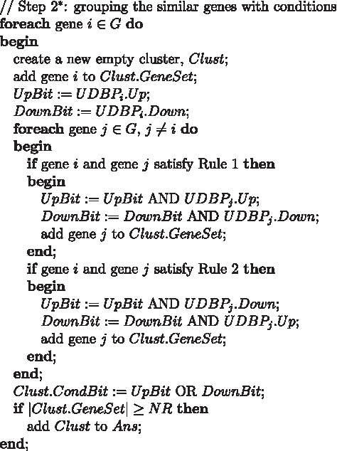
The new Step 2^*.

In Figure 7, initially, we create a new cluster, Clust. Then, for each gene i, we first add it to Clust.GeneSet. UpBit and DownBit are set to UDBP_i.Up and UDBP_i.Down, respectively. For each of the other genes, denoted as gene j, if it satisfies Rule 1 with gene i, we add gene j to Clust.GeneSet. Moreover, we update UpBit and DownBit by their AND results with UDBP_j.Up and UDBP_j.Down, respectively. If gene j satisfies Rule 2 with gene i, we add gene j to Clust.GeneSet. Moreover, we update UpBit and DownBit by their AND results with UDBP_j.Down and UDBP_j.Up, respectively. By this way, after all genes except gene i are checked, all genes similar to gene i are added to Clust.GeneSet. Moreover, the on-bits in UpBit and DownBit indicate those condition pairs where genes in Clust.GeneSet are coregulated (or negative-coregulated). Therefore, we let Clust.CondBit be the OR result of UpBit and DownBit. We can reversely derive the corresponding condition pair from each on-bit in Clust.CondBit to get those condition pairs where all genes in Clust.GeneSet are coregulated (or negative-coregulated).

Take the up-down bit patterns shown in Figure 6b as an example. Assume Sim = 0.9. First, we create a new cluster, Clust, and add gene 1 to Clust.GeneSet. UpBit and DownBit are now set to UDBP₁. Up ( = “111011”) and UDBP₁. Down ( = “000100”), respectively. Next, we check whether genes 2, 3, 4, and 5 can be added into this cluster. In this example, gene 2 satisfies Rule 1 with gene 1. Therefore, gene 2 is added into Clust.GeneSet. UpBit and DownBit are now set to their AND results with UDBP₂. Up and UDBP₂. Down , i.e., “111011” and “000100,” respectively. This means that genes 1 and 2 are coregulated under those condition pairs corresponding to on-bits in UpBit and DownBit. Gene 4 satisfies Rule 2 with gene 1. Therefore, gene 4 is added into Clust.GeneSet. UpBit and DownBit are now set to their AND results with UDBP₄. Down and UDBP₄. Up , i.e., “111011” and “000100,” respectively. This means that gene 4 is negative-coregulated to gene 1 under those condition pairs corresponding to on-bits in UpBit and DownBit. Genes 3 and 5 do not satisfy Rule 1 or Rule 2 with gene 1. After checking genes 2, 3, 4, and 5, UpBit is “111011” and DownBit is “000100.” Finally, we set Clust.CondBit to the OR result of UpBit and DownBit, i.e., Clust.CondBit = “111011” OR “000100” = “111111.” This means that genes in Clust.GeneSet, i.e., genes 1, 2, and 4, are coregulated or negative-coregulated under those condition pairs corresponding to the on-bits in “111111.” The corresponding condition pairs from the left to the right are (a → b), (a → c), (a → d), (b → c), (b → d), and (c → d) in order, as shown in Figure 6b. If NR (the minimal number of genes) is 3, Clust is a coregulated cluster and is added to Ans.

3.4. Step 3

In the previous step, we have found the clustering result stored in Ans according to parameters Sim (the similarity threshold) and NR (the minimal number of genes). In Step 3, we further present two post-processes for the found clusters which are to merge those similar clusters and to compute the similarity score of each cluster, respectively.

The process of Step 3 is shown in Figure 8. First, for every two clusters c1 and c2, if their gene sets overlap with each other by more than (MT × 100) percent, we merge them into a new cluster, where MT is the user-specified merging threshold and 0 ≤ MT ≤ 1. The purpose of this process is to reduce the number of clusters which may be redundant. Since the input data may be noisy, finding too many clusters with large overlaps only makes it difficult for the users to select those important clusters (Zhao and Zaki, 2005). In this case, the gene set of the new cluster is the union result of c1.GeneSet and c2.GeneSet. The bit string of condition pairs of the new cluster is the AND result of c1.CondBit and c2.CondBit. This process is optional for users. When MT is set to 1, the merging process will not be performed.

FIG. 8.

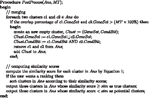
Step 3.

Next, we compute the similarity scores for clusters stored in Ans. For cluster x, its similarity score, SC(x), is evaluated by the following Equation 1: \documentclass{aastex} \usepackage{amsbsy} \usepackage{amsfonts} \usepackage{amssymb} \usepackage{bm} \usepackage{mathrsfs} \usepackage{pifont} \usepackage{stmaryrd} \usepackage{textcomp} \usepackage{portland, xspace} \usepackage{amsmath, amsxtra} \pagestyle{empty} \DeclareMathSizes {10} {9} {7} {6} \begin{document} \begin{align*} SC (x) = \mid x.CondBit \mid / {\rm C}^n_2. \tag{1} \end{align*} \end{document}

In other words, the similarity score is the percentage of on-bits in x.CondBit. This is because each on-bit represents one condition pair where all genes in x.GeneSet are coregulated. The more similar the genes of cluster x are to each other, the larger the number of on-bits in x.CondBit is.

After evaluating the similarity scores, we can provide a ranking for these clusters according to their similarity scores. There may exist clusters whose similarity scores are less than the similarity threshold, Sim. We call clusters whose similarity scores are not less than Sim as true clusters, and clusters whose similarity scores are less than Sim as potential clusters. The potential clusters are generated due to any of the following two processes: (1) Step 2/2^* and (2) merging. The reason for the first process (i.e., Step 2/2^*) has been mentioned previously. That is, we apply a heuristic method with time complexity O(m²) to find the clusters. Therefore, we may find some clusters whose genes do not completely satisfy the similarity threshold. For such clusters, instead of dropping them, we output them as potential clusters. This is because such clusters may still contain some biological meanings, although not every two genes within them satisfy the user-specified similarity threshold, Sim. The larger the number of genes in a found cluster which do not satisfy the threshold, the lower the similarity score of this cluster. Therefore, in Step 3 of the UDB method, we redeem the problem of those clusters which are generated in Step 2/2^* and do not satisfy the threshold by outputting them as potential clusters. The reason of generating potential clusters for the second process (i.e., merging) is that even if two clusters before merging satisfy the similarity threshold, there is no guarantee that the new cluster after merging will satisfy the similarity threshold. Therefore, although the merging process could reduce the number of redundant clusters, the number of true clusters may also decrease, i.e., a tradeoff.

4. Performance

In this section, we study the performance of the UDB method. We implemented the UDB method in Java, and performed all experiments on a Fedora Linux virtual machine (1024 MB of memory, an 2.4 GHz Intel processor) over Windows XP through VMware middleware.

4.1. Simulation results on synthetic data sets

In this subsection, we study the efficiency of the proposed UDB method by several synthetic data sets. Table 2 shows the related parameters for generating these synthetic data sets. Each synthetic data set is simulated by a 2-dimensional matrix with M rows and N columns. Then, X Co-gclusters with size (EM rows × EN columns) and \documentclass{aastex} \usepackage{amsbsy} \usepackage{amsfonts} \usepackage{amssymb} \usepackage{bm} \usepackage{mathrsfs} \usepackage{pifont} \usepackage{stmaryrd} \usepackage{textcomp} \usepackage{portland, xspace} \usepackage{amsmath, amsxtra} \pagestyle{empty} \DeclareMathSizes {10} {9} {7} {6} \begin{document} $$\epsilon = 0.5$$ \end{document} are randomly generated and embedded into the matrix. The rest of values of this matrix are random numbers. Table 3 shows three cases of the synthetic data sets. We will use these cases of data sets to study the efficiency of the proposed UDB method and compare it with the Co-gclustering method (Zhao et al., 2008).

Table 2.

Parameters Used in the Generation of Synthetic Data

Parameter	Description
M	Number of rows of the matrix
N	Number of columns of the matrix
X	Number of embedded Co-gclusters
EM	Number of rows of an embedded Co-gcluster
EN	Number of columns of an embedded Co-gcluster

Table 3.

Synthetic Data Sets

Case	M	N	X	EM	EN
1	3000–7000	22	5	0.02 × M	15
2	3000	18–22	10	50	15
3	3000	20	10	50	13–17

The default parameters for the Co-gclustering method and the UDB method are described as follows. The dissimilarity threshold in the Co-gclustering method is set to ∞ to find the same answers as the UDB method. The parameters of the minimal number of genes of a found cluster, i.e., α in the Co-gclustering method and NR in the UDB method, are set to the same value as EM. For the Co-gclustering method, the parameter of the minimal number of conditions of a found cluster, β, is set to EN. Since there does not exist such a parameter in the UDB method, we set the value of parameter Sim to ( \documentclass{aastex} \usepackage{amsbsy} \usepackage{amsfonts} \usepackage{amssymb} \usepackage{bm} \usepackage{mathrsfs} \usepackage{pifont} \usepackage{stmaryrd} \usepackage{textcomp} \usepackage{portland, xspace} \usepackage{amsmath, amsxtra} \pagestyle{empty} \DeclareMathSizes {10} {9} {7} {6} \begin{document} $${\rm C}^{\beta}_2 / {\rm C}^N_2$$ \end{document} ) to find the answers which contain the answers found by the Co-gclustering method. The reason is that if there exist genes coregulated under β conditions, the corresponding \documentclass{aastex} \usepackage{amsbsy} \usepackage{amsfonts} \usepackage{amssymb} \usepackage{bm} \usepackage{mathrsfs} \usepackage{pifont} \usepackage{stmaryrd} \usepackage{textcomp} \usepackage{portland, xspace} \usepackage{amsmath, amsxtra} \pagestyle{empty} \DeclareMathSizes {10} {9} {7} {6} \begin{document} $${\rm C}^{\beta}_2$$ \end{document} bits for these β conditions in up-down bit patterns (whose lengthes are all \documentclass{aastex} \usepackage{amsbsy} \usepackage{amsfonts} \usepackage{amssymb} \usepackage{bm} \usepackage{mathrsfs} \usepackage{pifont} \usepackage{stmaryrd} \usepackage{textcomp} \usepackage{portland, xspace} \usepackage{amsmath, amsxtra} \pagestyle{empty} \DeclareMathSizes {10} {9} {7} {6} \begin{document} $${\rm C}^N_2$$ \end{document} ) must be all on-bits. Note that we will find more answers than the Co-gclustering method when \documentclass{aastex} \usepackage{amsbsy} \usepackage{amsfonts} \usepackage{amssymb} \usepackage{bm} \usepackage{mathrsfs} \usepackage{pifont} \usepackage{stmaryrd} \usepackage{textcomp} \usepackage{portland, xspace} \usepackage{amsmath, amsxtra} \pagestyle{empty} \DeclareMathSizes {10} {9} {7} {6} \begin{document} $$Sim = {\rm C}^{\beta}_2 / {\rm C}^N_2$$ \end{document} . This is because there may exist genes coregulated under only some condition pairs, instead of all conditions in those condition pairs. For example, there may exist genes coregulated under only condition pairs (a → b), (a → c), and (a → d), instead of all of these conditions (i.e., a, b, c, and d).

For the data set of Case 1, we study the relationship between the processing time and the number of genes in a microarray data set, and make a comparison between the Co-gclustering method and the UDB method. Figure 9 shows the simulation result for the data set of Case 1. From this figure, we could observe that the processing time of the UDB method increases as the number of genes (i.e., M) increases, since the time complexity of the UDB method is O (M²). Moreover, the UDB method needs shorter processing time than the Co-gclustering method for this data set. The reason is that the number of conditions greatly affects the processing time of the Co-gclustering method. In this simulation, such an effect makes the Co-gclustering method need longer processing time than the UDB method even when the number of genes is large.

FIG. 9.

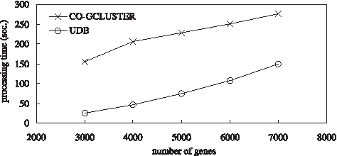
A comparison of the processing time for the data set of Case 1.

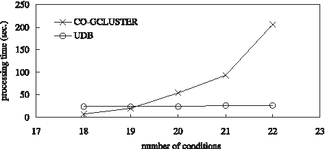
For the data set of Case 2, we study the relationship between the processing time and the number of conditions in a microarray data set, and compare the processing time of the UDB method with that of the Co-gclustering method. Figure 10 shows the simulation result for the data set of Case 2. From this figure, we can observe that the UDB method needs shorter processing time than the Co-gclustering method for this data set. In Figure 10, the processing time of the Co-gclustering method seems to increase exponentially as the number of conditions (i.e., N) increases, since its time complexity is O(2^N). Although the processing time of the Co-gclustering method may be shorter than that of the UDB method when the value of N is small, it increases quickly as the value of N increases. On the other hand, the processing time of the UDB method does not have obvious variations as the number of conditions increases. The reason is that the number of conditions only affects the length (i.e., \documentclass{aastex} \usepackage{amsbsy} \usepackage{amsfonts} \usepackage{amssymb} \usepackage{bm} \usepackage{mathrsfs} \usepackage{pifont} \usepackage{stmaryrd} \usepackage{textcomp} \usepackage{portland, xspace} \usepackage{amsmath, amsxtra} \pagestyle{empty} \DeclareMathSizes {10} {9} {7} {6} \begin{document} $${\rm C}^N_2$$ \end{document} ) and the generation (i.e., Step 1 of the UDB method) of a up/down bit pattern. The time complexity of Step 1 of the UDB method is O(M × N²). However, since the value of N is much smaller than the value of M, the effect of varying the value of N is of little concern to the processing time of the UDB method.

FIG. 10.

A comparison of the processing time for the data set of Case 2.

For the data set of Case 3, we study the relationship between the processing time and the number of conditions in a found Co-gcluster (i.e., EN), and make a comparison between the Co-gclustering method and the UDB method. For the Co-gclustering method, the parameter of the minimal number of conditions of a Co-gcluster, β, is set to 12. Parameter Sim in the UDB method is set to \documentclass{aastex} \usepackage{amsbsy} \usepackage{amsfonts} \usepackage{amssymb} \usepackage{bm} \usepackage{mathrsfs} \usepackage{pifont} \usepackage{stmaryrd} \usepackage{textcomp} \usepackage{portland, xspace} \usepackage{amsmath, amsxtra} \pagestyle{empty} \DeclareMathSizes {10} {9} {7} {6} \begin{document} $$({\rm C}^{\beta}_2 / {\rm C}^N_2 ) = ({\rm C}^{12}_2 / {\rm C}^{20}_2) = 0.34$$ \end{document} . Figure 11 shows the simulation result for the data set of Case 3. From this figure, we could observe that the UDB method needs shorter processing time than the Co-gclustering method for this data set. The processing time of the Co-gclustering method also seems to increase exponentially as the value of EN increases. The reason is that as the value of EN increases, to find all clusters, both the number of trees and the size of trees needed to be generated in the Co-gclustering method also increase. The processing time of the UDB method does not have obvious variations as the value of EN increases. The reason is that no matter what value the number of conditions in a found cluster is, the UDB method always utilizes the same loop with time complexity O(M²) to find all clusters.

FIG. 11.

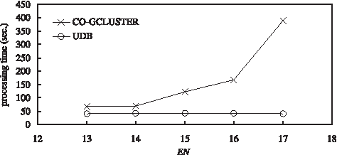
A comparison of the processing time for the data set of Case 3.

4.2. Experimental results on real data sets

In this subsection, first, we use real microarray data sets as the experimental data to study the efficiency of the proposed method. Table 4 shows the real microarray data sets used in the experiments. The yeast microarray data set (Tavazoie et al., 1999), obtained from the yeast Saccharomyces Cerevisiae cell cycle expression levels, is widely used in microarray clustering research. The ALL-AML microarray data set (Brunet et al., 2004), often used in microarray classification research, is composed of samples from 27 ALL (acute lymphoblastic leukemia) patients and 11 AML (acute myeloid leukemia) patients. The breast microarray (West et al., 2001) consists of 49 breast cancer samples, obtained from the Duke Breast Cancer SPORE frozen tissue bank.

Table 4.

Real Microarray Data Sets

Name	Number of genes	Number of samples
Yeast	2884	17
ALL-AML	5000	38
Breast	7129	49

Table 5 shows the experimental results of these three data sets. From this figure, we could observe that the UDB method needs shorter processing time than the Co-gclustering method for these data sets. The reason is that the UDB method is a polynomial-time method, while the Co-gclustering method is an exponential-time method. The ALL-AML data set consists of more genes and more samples than the yeast data set, and the breast data set consists of more genes and more samples than the ALL-AML data set. Since the time complexity of the UDB method is O(M²) (where M is the number of genes), the processing time of the UDB method for these three data sets increases progressively. However, the processing time of the Co-gclustering method grows exponentially to the number of conditions. Therefore, we could observe that as the number of conditions among these data sets increases, the difference of the processing time between the Co-gclustering method and the UDB method also increases.

Table 5.

Experimental Results for Real Microarray Data Sets

Data set	\documentclass{aastex} \usepackage{amsbsy} \usepackage{amsfonts} \usepackage{amssymb} \usepackage{bm} \usepackage{mathrsfs} \usepackage{pifont} \usepackage{stmaryrd} \usepackage{textcomp} \usepackage{portland, xspace} \usepackage{amsmath, amsxtra} \pagestyle{empty} \DeclareMathSizes {10} {9} {7} {6} \begin{document} $$\epsilon$$ \end{document}	α(NR)	\documentclass{aastex} \usepackage{amsbsy} \usepackage{amsfonts} \usepackage{amssymb} \usepackage{bm} \usepackage{mathrsfs} \usepackage{pifont} \usepackage{stmaryrd} \usepackage{textcomp} \usepackage{portland, xspace} \usepackage{amsmath, amsxtra} \pagestyle{empty} \DeclareMathSizes {10} {9} {7} {6} \begin{document} $$\beta ((Sim == {C}^ \beta_2 {C}^N_2 ))$$ \end{document}	UDB (sec)	Co-gclustering (sec)
Yeast	0.01	80	9	46.3	94.3
		50	10	47.7	102.5
		30	11	52.1	126
ALL-AML	0.95	250	3	102.8	251.7
		100	4	109.7	254.7
		50	5	141.42	252.9
Breast	1.45	500	3	289.9	1065.8
		300	4	423.9	1058.4
		80	5	469.5	1064.2

Next, we discuss the correlation of genes in clusters found by the UDB method. We use the yeast microarray data set (composed of 2884 rows and 17 columns) as the experimental data set. For the UDB method, when parameters are set to \documentclass{aastex} \usepackage{amsbsy} \usepackage{amsfonts} \usepackage{amssymb} \usepackage{bm} \usepackage{mathrsfs} \usepackage{pifont} \usepackage{stmaryrd} \usepackage{textcomp} \usepackage{portland, xspace} \usepackage{amsmath, amsxtra} \pagestyle{empty} \DeclareMathSizes {10} {9} {7} {6} \begin{document} $$\epsilon = 0.05, NR = 30,$$ \end{document} and Sim = 0.75, there are 6 clusters found from this data set. For the found clusters, we utilize a Gene Ontology (GO) annotation searching tool, GO Term Finder (www.yeastgenome.org/cgi-bin/GO/goTermFinder.pl), to verify their biological meaning. The GO project provides a controlled vocabulary to describe gene and gene product attributes in any organism, and is a collaborative effort to address the need for consistent descriptions of gene products in different databases (cited from www.geneontology.org). With this tool, we can find the significant shared GO terms for genes within the same cluster. Table 6 shows the searching result of GO terms for these 6 clusters. For each ontology, we list only the significant shared term with the smallest p-value (which is smaller than 0.01), where a p-value is a score of significance. The closer the p-value is to zero, the more significant is the particular GO term associated with the group of genes (cited from www.yeastgenome.org). From Table 6, we could observe that genes within the same cluster significantly share the same GO terms, which means that these genes jointly participate in some activities.

Table 6.

Searching Result of GO Terms for Clusters Found by the UDB Method

No. of genes in this cluster	No. of genes belong to the GO term	Ontology	GO term	p-Value
33	15	Process	Cellular response to DNA damage stimulus	1.52 × 10⁻¹²
	5	Function	Double-stranded DNA binding	2.42 × 10⁻⁰⁵
	9	Component	Replication fork	7.87 × 10⁻¹²
31	18	Process	DNA metabolic process	2.34 × 10⁻¹³
	4	Function	Double-stranded DNA binding	0.00046
	15	Component	Chromosome	3.68 × 10⁻¹¹
31	14	Process	Cellular response to DNA damage stimulus	1.22 × 10⁻¹¹
	4	Function	Chromatin binding	0.00285
	7	Component	Replication fork	1.93 × 10⁻⁸
32	15	Process	Cell cycle	5.28 × 10⁻⁸
	4	Function	Chromatin binding	0.00324
	3	Component	Mitotic cohesin complex	2.22 × 10⁻⁵
33	15	Process	Cell cycle	9.43 × 10⁻⁸
	4	Function	Chromatin binding	0.00388
	11	Component	Nuclear chromosome	7.33 × 10⁻⁷
30	15	Process	DNA metabolic process	1.1 × 10⁻⁹
	11	Component	Chromosomal part	5.25 × 10⁻⁷

We then try to find the corresponding Co-gclusters by the Co-gclustering method with equivalent parameters. These equivalent parameters are described as follow. The values of \documentclass{aastex} \usepackage{amsbsy} \usepackage{amsfonts} \usepackage{amssymb} \usepackage{bm} \usepackage{mathrsfs} \usepackage{pifont} \usepackage{stmaryrd} \usepackage{textcomp} \usepackage{portland, xspace} \usepackage{amsmath, amsxtra} \pagestyle{empty} \DeclareMathSizes {10} {9} {7} {6} \begin{document} $$\epsilon$$ \end{document} and α in the Co-gclustering method are set to the same values of \documentclass{aastex} \usepackage{amsbsy} \usepackage{amsfonts} \usepackage{amssymb} \usepackage{bm} \usepackage{mathrsfs} \usepackage{pifont} \usepackage{stmaryrd} \usepackage{textcomp} \usepackage{portland, xspace} \usepackage{amsmath, amsxtra} \pagestyle{empty} \DeclareMathSizes {10} {9} {7} {6} \begin{document} $$\epsilon$$ \end{document} and NR in the UDB method, i.e., 0.05 and 30, respectively. As we mentioned in the previous subsection, since the value of Sim is equal to ( \documentclass{aastex} \usepackage{amsbsy} \usepackage{amsfonts} \usepackage{amssymb} \usepackage{bm} \usepackage{mathrsfs} \usepackage{pifont} \usepackage{stmaryrd} \usepackage{textcomp} \usepackage{portland, xspace} \usepackage{amsmath, amsxtra} \pagestyle{empty} \DeclareMathSizes {10} {9} {7} {6} \begin{document} $${\rm C}^{\beta}_2 / {\rm C}^N_2$$ \end{document} ), the value of β is set to \documentclass{aastex} \usepackage{amsbsy} \usepackage{amsfonts} \usepackage{amssymb} \usepackage{bm} \usepackage{mathrsfs} \usepackage{pifont} \usepackage{stmaryrd} \usepackage{textcomp} \usepackage{portland, xspace} \usepackage{amsmath, amsxtra} \pagestyle{empty} \DeclareMathSizes {10} {9} {7} {6} \begin{document} $$(1 + \sqrt{1 + 4 \times Sim \times N \times (N - 1)}) / 2 = (1 + \sqrt{1 + 4 \times 0.75 \times 17 \times16}) / 2 = 14$$ \end{document} . However, with such values of parameters, the Co-gclustering method can not find any cluster. The reason is that as we mentioned in the previous subsection, there may exist genes coregulated under only some condition pairs, instead of all conditions in those condition pairs. In this experiment, although there do not exist genes coregulated under at least β = 14 samples, there may exist genes coregulated under at least (Sim × 100 = 75) percent of condition pairs. Therefore, the UDB method may find some interesting clusters which can not be found by the Co-gclustering method.

5. Conclusion

Biclustering of microarray data has been shown to be instrumental in microarray data analysis. In this article, we have proposed the UDB method, which can efficiently find clusters with correlated and negative-correlated patterns. The UDB method utilizes up-down bit patterns to record those condition pairs where one gene is upregulated or downregulated. Then, by applying a heuristic idea on these up-down bit patterns, we can find all clusters in polynomial time. From the simulation results on synthetic microarray data sets, we have studied the factors in the data sets which affect the processing time of the UDB method. Moreover, from the experimental results on synthetic and real microarray data sets, we have shown that the UDB method is more efficient than the Co-gclustering method. Furthermore, we have shown the correlation of genes in clusters found by the UDB method for the yeast microarray data set.

Footnotes

Acknowledgments

This research was supported in part by the National Science Council of Republic of China (Grant NSC-95-2221-E-110-079-MY2) and by the “Aim for Top University Plan” project of NSYSU and the Ministry of Education, Taiwan.

Disclosure Statement

No competing financial interests exist.

References

Aguilar-Ruiz

J.S.

2005. Shifting and scaling patterns from gene expression data. Bioinformatics, 21:3840–3845.

Ben-Dor

, Chor

, Karp

R.M.

et al. 2003. Discovering local structure in gene expression data: the order-preserving submatrix problem. J. Comput. Biol., 10:373–384.

Breitkreutz

B.J.

, Stark

, Tyers

2006. Yeast grid. http://biodata.mshri.on.ca/yeast_grid/servlet/. 2010 October 1.

Brunet

J.P.

, Tamayo

, Golub

T.R.

et al. 2004. Metagenes and molecular pattern discovery using matrix factorization. Proc. Natl. Acad. Sci. USA, 4164–4169.

Chang

Y.I.

, Chen

J.R.

, Tsai

Y.C.

2009. Mining subspace clusters from DNA microarray data using large itemset techniques. J. Comput. Biol., 16:745–768.

Cheng

, Church

G.M.

2000. Biclustering of expression data. Proc. 8th Int. Conf. Intell. Syst. Mol. Biol., 93–103.

Ihmels

, Bergmann

, Barkai

2004. Defining transcription modules using large-scale gene expression data. Bioinformatics, 20:1993–2003.

Liu

, Wang

2003. Op-Cluster: clustering by tendency in high-dimensional space. Proc. 3rd IEEE Int. Conf. Data Mining, 187–194.

Madeira

S.C.

, Oliveira

A.L.

2004. Biclustering algorithms for biological data analysis: a survey. IEEE/ACM Trans. Comput. Biol. Bioinform., 1:24–45.

10.

Okada

, Fujibuchi

, Horton

2007. A biclustering method for gene expression module discovery using a closed itemset enumeration algorithm. IPSJ Digital Courier, 3:183–192.

11.

Tanay

, Sharan

, Shamir

2002. Discovering statistically significant biclusters in gene expression data. Bioinformatics, 18:136–144.

12.

Tavazoie

, Hughes

J.D.

, Campbell

M.J.

et al. 1999. Systematic determination of genetic network architecture. Nat. Genet., 22:281–285.

13.

Wang

, Wang

, Yang

et al. 2002. Clustering by pattern similarity in large data sets. Proc. ACM SIGMOD Int. Conf. Manage. Data, 394–405.

14.

West

, Blanchette

, Dressman

et al. 2001. Predicting the clinical status of human breast cancer using gene expression profiles. Proc. Natl. Acad. Sci. USA, 11462–11467.

15.

Yang

, Wang

et al. 2005. An improved biclustering method for analyzing gene expression profiles. Int. J. Artif. Intell. Tools, 14:771–789.

16.

Yoon

, Nardini

, Benini

et al. 2005. Discovering coherent biclusters from gene expression data using zero-suppressed binary decision diagrams. IEEE/ACM Trans. Comput. Biol. Bioinform., 2:339–354.

17.

Zhao

, Zaki

M.J.

2005. MicroCluster: efficient deterministic biclustering of microarray data. IEEE Intell. Syst., 20:40–49.

18.

Zhao

, Yu

J.X.

, Wang

et al. 2008. Maximal subspace coregulated gene clustering. IEEE Trans. Knowl. Data Eng., 20:83–98.