Maximum Parsimony,Substitution Model,and Probability Phylogenetic Trees

Abstract

The problem of inferring phylogenies (phylogenetic trees) is one of the main problems in computational biology. There are three main methods for inferring phylogenies—Maximum Parsimony (MP), Distance Matrix (DM) and Maximum Likelihood (ML), of which the MP method is the most well-studied and popular method. In the MP method the optimization criterion is the number of substitutions of the nucleotides computed by the differences in the investigated nucleotide sequences. However, the MP method is often criticized as it only counts the substitutions observable at the current time and all the unobservable substitutions that really occur in the evolutionary history are omitted. In order to take into account the unobservable substitutions, some substitution models have been established and they are now widely used in the DM and ML methods but these substitution models cannot be used within the classical MP method. Recently the authors proposed a probability representation model for phylogenetic trees and the reconstructed trees in this model are called probability phylogenetic trees. One of the advantages of the probability representation model is that it can include a substitution model to infer phylogenetic trees based on the MP principle. In this paper we explain how to use a substitution model in the reconstruction of probability phylogenetic trees and show the advantage of this approach with examples.

1. Introduction

Phylogeny reconstruction, or the inference of phylogenies from bio-sequences (nucleotide or protein sequences) is an old (dating from Darwin's evolutionary theory) and intensively studied problem in computational biology. Given a set N of organisms the phylogeny problem asks for a network T on N that represents the evolutionary history of, and the interrelationships among, these biological entities. Many methods for reconstructing phylogenies have been proposed, and all of them assume that the network T is a bifurcating tree, called a phylogenetic tree, because multi-furcation can be treated as two bifurcations that are sufficiently close together. All given organisms in T are leaves (called tips or terminals) of T while the common ancestor r of all organisms in the given set is the root of T although in many studies the tree is treated as unrooted. Actually, any internal node is the root of a subtree of T whose leaves are the descendants of this internal node (Felsenstein, 2004). The graph structure of a network is called its topology. In particular, if the degree of any node in the network is no more than three, then the topology is called a Steiner topology in the literature on network optimisation. (The reason for the use of this term is that the shortest network problem was historically named the Steiner tree problem [Hwang, 1992].) Moreover, a tree with a Steiner topology is called a Steiner tree, the nodes not in the given input set are called Steiner points. A Steiner topology is full if all nodes in the input set are terminals (nodes of degree one). Hence, a phylogenetic tree T is a tree with a full Steiner topology.

The reconstruction of phylogenetic trees is based on nucleotide or protein sequences (bio-sequences). In this article, the sequences we study are uncoded nucleotide sequences that consist of characters from the alphabet {A,C,G,T} but all the arguments can be applied to proteins or other kind of sequences. Of all the methods developed for phylogenies—such as Maximum Parsimony (MP), Distance Matrix (DM), and Maximum Likelihood (ML)—the MP method is the most well- studied and popular method because of its simplicity. The principle of Maximum Parsimony is like Ockham's razor: in the absence of contrary information, the simplest is the best, i.e., the simplest manipulations of the observed data are the best explanation for the data. In the case of inferring phylogenies, this principle can be described as “evolution is parsimonious.” Specifically, the amount of evolutionary change (the total number of substitutions of nucleotides) is minimized. The MP method relies on directly observable changes in the input bio-sequences. Although the MP method continues to be widely used, it is often criticized as not being statistically sound, i.e., there is a lack of assumption involving an underlying substitution model (Steel, 2000). The reason for this is that the actual substitution patterns are very complicated: In the evolutionary process there exist multi-, parallel-, convergent-, and back-substitutions (Xia, 2006). Multi-substitutions result in the number of observable substitutions being less than the actual occurring multi-substitutions, while the last three kinds of substitutions mentioned above cannot be observed at all in the comparison of sequences. The cost of the simplicity of the MP method is that these unobserved substitutions are ignored and the number of observable substitutions typically greatly underestimates the actual number of substitutions in the evolutionary history. In order to reflect these invisible substitutions, a number of substitution models such as the Jukes-Cantor model (Jukes et al., 1969) have been developed (Ewens et al., 2005). These substitution models are now widely used in the DM and ML methods. However, because the MP method is character-based and because it cannot take into account different possible substitutions on an edge simultaneously, the substitution models cannot be applied in the classical MP method.

The existing MP method is deterministic in the sense that any internal node at a site is determined as an “either this or that” nucleotide. Because an evolutionary history cannot be repeated, we are unable to know exactly the ancestors of a given set of organisms. Hence, a more logical approach is to assume that each site of an internal node is a probability distribution of the four types of nucleotide. For instance, if the distribution on a site of a node is [A,C,G,T] = [0.80, 0.18, 0.01, 0.01], then we can say that during the evolutionary history the nucleotide on this site was most likely to be A, with a small probability it was C, but it was most unlikely to be G or T. Based on this argument the authors have recently proposed a probability presentation model of phylogenetic trees and the trees constructed in this model are called probability phylogenetic trees (Weng et al., 2008). The probability representation model makes it possible to use a substitution model in reconstructing probability phylogenetic trees by the MP principle. In this article, we explain this new approach and, using examples, show the advantage of the proposed approach over the classical MP method.

2. Probability Phylogenetic Model and Statistical Distance

The problem of reconstructing phylogenies is closely related to the Steiner tree problem, a well-studied problem in combinatorial optimization (Foulds et al., 1982; Brazil et al., 2009). The classical Steiner tree problem has two versions: in graphs or in metric spaces. The probability representation model is related to the real d-dimensional space version whose mathematical formulation is as follows:

Given: A set N of points in a vector space \documentclass{aastex}\usepackage{amsbsy}\usepackage{amsfonts}\usepackage{amssymb}\usepackage{bm}\usepackage{mathrsfs}\usepackage{pifont}\usepackage{stmaryrd}\usepackage{textcomp}\usepackage{portland,xspace}\usepackage{amsmath,amsxtra}\pagestyle{empty}\DeclareMathSizes{10}{9}{7}{6} \begin{document} \begin{align*} {\cal S} \end{align*} \end{document} , a length function f_ℓ(e) and a weight function w(e) of edge e.

Objective: Find the optimal network T spanning N such that the weighted length of the tree \documentclass{aastex}\usepackage{amsbsy}\usepackage{amsfonts}\usepackage{amssymb}\usepackage{bm}\usepackage{mathrsfs}\usepackage{pifont}\usepackage{stmaryrd}\usepackage{textcomp}\usepackage{portland,xspace}\usepackage{amsmath,amsxtra}\pagestyle{empty}\DeclareMathSizes{10}{9}{7}{6} \begin{document} \begin{align*} L ( T ) = \sum_{{ \bf e} \in E ( T ) } w ( { \bf e} ) f_ \ell ( { \bf e} ) = \sum_{pq \in E ( T ) } w ( { \bf p} , { \bf q} ) f_ \ell ( pq ) \end{align*} \end{document}

is minimized, where E(T) is the edge set of T, w_e is the weight of edge e and p, q are the endpoints of the edge.

Due to minimality, the optimal network T does not contain cycles. That is, T has a tree topology, and hence, T is called a Steiner minimal tree. There are two “levels” of optimisation of T in the Steiner tree problem. T is locally optimal if it is optimal with respect to a fixed topology, i.e., optimal over all networks with the same topology, while T is globally optimal if it is optimal over all feasible topologies. In this article, our focus is mainly on local optimisation although the comparison of topologies on the global optimisation level is also discussed in Example 3 in Section 4.

A vector v is called a probability vector if each component v_i of v satisfies 0 ≤ v_i ≤ 1 and Σ_iv_i = 1. A matrix is a probability matrix if each row (or each column) is a probability vector. A tree is a probability tree if the nodes in the tree are all probability vectors (or probability matrices). Hence, the probability Steiner tree problem is an optimisation problem with a probability vector constraint, and the optimal solution is called a probability Steiner minimal tree.

Note that when a sequence is produced in a wet laboratory, it may contain uncertain characters (ambiguous characters). Besides, gaps may occur due to insertion/deletion of characters in alignment. Moreover, in the reconstruction of phylogenetic trees using the MP method, an optimal assignment of internal nodes on each site, called an evolutionary pathway on the site, is often not unique. Due to this non-uniqueness, for a fixed site the length of an edge is defined to be the average of the numbers of substitutions over all evolutionary pathways. The ambiguity in the input sequences and the non-uniqueness of the output have lead us to consider the probability presentation model. More importantly, as we have stated in the first section, the evolutionary history of a given set of species is not repeatable and we cannot precisely infer the ancestors of the species. Hence, instead of a determinate assignment of nucleotides to an internal node in pathways, in the probability representation model of phylogenetic trees a distribution of the nucleotide states will be inferred for each site of each internal node. The probability representation model consists of two steps:

converting all nucleotide sequences in the input set N into probability vector sequences, consequently the input becomes a set N of probability matrices, and

constructing a probability phylogenetic tree T that is actually a probability Steiner minimal tree spanning the input set N of probability matrices.

Let T be the phylogenetic tree on a set N of n nucleotide sequences of equal length m, and T^k be the tree constrained to site k. First we map all characters (nucleotides or non-nucleotide characters) in the input sequences to points in a 4-dimensional probability vector space \documentclass{aastex}\usepackage{amsbsy}\usepackage{amsfonts}\usepackage{amssymb}\usepackage{bm}\usepackage{mathrsfs}\usepackage{pifont}\usepackage{stmaryrd}\usepackage{textcomp}\usepackage{portland,xspace}\usepackage{amsmath,amsxtra}\pagestyle{empty}\DeclareMathSizes{10}{9}{7}{6} \begin{document} \begin{align*} { \cal S} \end{align*} \end{document} . The four types of nucleotides form the basis of \documentclass{aastex}\usepackage{amsbsy}\usepackage{amsfonts}\usepackage{amssymb}\usepackage{bm}\usepackage{mathrsfs}\usepackage{pifont}\usepackage{stmaryrd}\usepackage{textcomp}\usepackage{portland,xspace}\usepackage{amsmath,amsxtra}\pagestyle{empty}\DeclareMathSizes{10}{9}{7}{6} \begin{document} \begin{align*} { \cal S} \end{align*} \end{document} : \documentclass{aastex}\usepackage{amsbsy}\usepackage{amsfonts}\usepackage{amssymb}\usepackage{bm}\usepackage{mathrsfs}\usepackage{pifont}\usepackage{stmaryrd}\usepackage{textcomp}\usepackage{portland,xspace}\usepackage{amsmath,amsxtra}\pagestyle{empty}\DeclareMathSizes{10}{9}{7}{6} \begin{document} \begin{align*} { \rm A} = [ 1 , 0 , 0 , 0 ] , \ { \rm C} = [ 0 , 1 , 0 , 0 ] , \ { \rm G} = [ 0 , 0 , 0 , 1 ] , \ { \rm T} = [ 0 , 0 , 0 , 1 ]. \end{align*} \end{document}

All other non-nucleotide characters (uncertain characters and gaps) need to be determined using particular methods. For example, in Example 2 (see Section 4 below) the character on site 6 in the sequence of Turkey is “N,” a character in the table of the IUPAC-IUB Commission on Biochemical Nomenclature (Liébecq, 1992), meaning an A, or C, or G, or T, i.e. any nucleotide is possible. Therefore, we will assume the probability distribution is [0.25,0.25,0.25,0.25] if no bias is given beforehand. Once the distributions of all non-nucleotide characters are determined, then a nucleotide sequence \documentclass{aastex}\usepackage{amsbsy}\usepackage{amsfonts}\usepackage{amssymb}\usepackage{bm}\usepackage{mathrsfs}\usepackage{pifont}\usepackage{stmaryrd}\usepackage{textcomp}\usepackage{portland,xspace}\usepackage{amsmath,amsxtra}\pagestyle{empty}\DeclareMathSizes{10}{9}{7}{6} \begin{document} \begin{align*} { \rm P} = { \rm p}^1{ \rm p}^2 \ldots { \rm p}^m \end{align*} \end{document} of length m is translated into a 4 × m probability matrix \documentclass{aastex}\usepackage{amsbsy}\usepackage{amsfonts}\usepackage{amssymb}\usepackage{bm}\usepackage{mathrsfs}\usepackage{pifont}\usepackage{stmaryrd}\usepackage{textcomp}\usepackage{portland,xspace}\usepackage{amsmath,amsxtra}\pagestyle{empty}\DeclareMathSizes{10}{9}{7}{6} \begin{document} \begin{align*} { \bf P} = \Big [ p_j^k \Big ] = \Big [ { \bf p}^1 { \bf p}^2 \cdots { \bf p}^m \Big ] , 0 \le p_j^k \le 1 , \sum_{j\ =\ 1}^4 p_j^k = 1 , k = 1 , \cdots , m , \end{align*} \end{document}

such that each column \documentclass{aastex}\usepackage{amsbsy}\usepackage{amsfonts}\usepackage{amssymb}\usepackage{bm}\usepackage{mathrsfs}\usepackage{pifont}\usepackage{stmaryrd}\usepackage{textcomp}\usepackage{portland,xspace}\usepackage{amsmath,amsxtra}\pagestyle{empty}\DeclareMathSizes{10}{9}{7}{6} \begin{document} \begin{align*} { \bf p}^k = \Big [ p_1^k \ p_2^k \ p_3^k \ p_4^k \Big ] ^T \ ( k = 1 , 2 , \cdots , m ) \end{align*} \end{document} in P is a probability vector in \documentclass{aastex}\usepackage{amsbsy}\usepackage{amsfonts}\usepackage{amssymb}\usepackage{bm}\usepackage{mathrsfs}\usepackage{pifont}\usepackage{stmaryrd}\usepackage{textcomp}\usepackage{portland,xspace}\usepackage{amsmath,amsxtra}\pagestyle{empty}\DeclareMathSizes{10}{9}{7}{6} \begin{document} \begin{align*} {\cal S} \end{align*} \end{document} . That is, we establish a correspondence between \documentclass{aastex}\usepackage{amsbsy}\usepackage{amsfonts}\usepackage{amssymb}\usepackage{bm}\usepackage{mathrsfs}\usepackage{pifont}\usepackage{stmaryrd}\usepackage{textcomp}\usepackage{portland,xspace}\usepackage{amsmath,amsxtra}\pagestyle{empty}\DeclareMathSizes{10}{9}{7}{6} \begin{document} \begin{align*} { \rm P} = { \rm p}^1{ \rm p}^2 \ldots { \rm p}^m \end{align*} \end{document} and \documentclass{aastex}\usepackage{amsbsy}\usepackage{amsfonts}\usepackage{amssymb}\usepackage{bm}\usepackage{mathrsfs}\usepackage{pifont}\usepackage{stmaryrd}\usepackage{textcomp}\usepackage{portland,xspace}\usepackage{amsmath,amsxtra}\pagestyle{empty}\DeclareMathSizes{10}{9}{7}{6} \begin{document} \begin{align*} { \bf P} = { \bf p}^1 { \bf p}^2 \ldots { \bf p}^m \end{align*} \end{document} such that pⁱ ⇔ pⁱ, \documentclass{aastex}\usepackage{amsbsy}\usepackage{amsfonts}\usepackage{amssymb}\usepackage{bm}\usepackage{mathrsfs}\usepackage{pifont}\usepackage{stmaryrd}\usepackage{textcomp}\usepackage{portland,xspace}\usepackage{amsmath,amsxtra}\pagestyle{empty}\DeclareMathSizes{10}{9}{7}{6} \begin{document} \begin{align*} i = 1 , 2 , \ldots , m \end{align*} \end{document} . For example, the sequence AAGCTNG \documentclass{aastex}\usepackage{amsbsy}\usepackage{amsfonts}\usepackage{amssymb}\usepackage{bm}\usepackage{mathrsfs}\usepackage{pifont}\usepackage{stmaryrd}\usepackage{textcomp}\usepackage{portland,xspace}\usepackage{amsmath,amsxtra}\pagestyle{empty}\DeclareMathSizes{10}{9}{7}{6} \begin{document} \begin{align*} \cdots \end{align*} \end{document} for Turkey in Example 2 (see Section 4 below) is translated into a probability matrix \documentclass{aastex}\usepackage{amsbsy}\usepackage{amsfonts}\usepackage{amssymb}\usepackage{bm}\usepackage{mathrsfs}\usepackage{pifont}\usepackage{stmaryrd}\usepackage{textcomp}\usepackage{portland,xspace}\usepackage{amsmath,amsxtra}\pagestyle{empty}\DeclareMathSizes{10}{9}{7}{6} \begin{document} \begin{align*} \left( \begin{matrix}1 & 1 & 0 & 0 & 0 & 0.25 & 0 & \cdots \\ 0 & 0 & 0 & 1 & 0 & 0.25 & 0 & \cdots \\ 0 & 0 & 1 & 0 & 0 & 0.25 & 1 & \cdots \\ 0 & 0 & 0 & 0 & 1 & 0.25 & 0 & \cdots \end{matrix} \right). \end{align*} \end{document}

Remark 2.1.

(1) In the notation \documentclass{aastex}\usepackage{amsbsy}\usepackage{amsfonts}\usepackage{amssymb}\usepackage{bm}\usepackage{mathrsfs}\usepackage{pifont}\usepackage{stmaryrd}\usepackage{textcomp}\usepackage{portland,xspace}\usepackage{amsmath,amsxtra}\pagestyle{empty}\DeclareMathSizes{10}{9}{7}{6} \begin{document} \begin{align} p_j^k \end{align} \end{document} the subscript j denotes the row while the superscript k denotes the column where \documentclass{aastex}\usepackage{amsbsy}\usepackage{amsfonts}\usepackage{amssymb}\usepackage{bm}\usepackage{mathrsfs}\usepackage{pifont}\usepackage{stmaryrd}\usepackage{textcomp}\usepackage{portland,xspace}\usepackage{amsmath,amsxtra}\pagestyle{empty}\DeclareMathSizes{10}{9}{7}{6} \begin{document} \begin{align} p_j^k \end{align} \end{document} is located. The superscript T in [ · ]^T denotes the transposition of vectors.

(2) We use \documentclass{aastex}\usepackage{amsbsy}\usepackage{amsfonts}\usepackage{amssymb}\usepackage{bm}\usepackage{mathrsfs}\usepackage{pifont}\usepackage{stmaryrd}\usepackage{textcomp}\usepackage{portland,xspace}\usepackage{amsmath,amsxtra}\pagestyle{empty}\DeclareMathSizes{10}{9}{7}{6} \begin{document} \begin{align} { \rm N} , { \rm T} , { \rm P} , { \rm p} , \ldots \end{align} \end{document} to denote discrete variables for bio-sequences and use \documentclass{aastex}\usepackage{amsbsy}\usepackage{amsfonts}\usepackage{amssymb}\usepackage{bm}\usepackage{mathrsfs}\usepackage{pifont}\usepackage{stmaryrd}\usepackage{textcomp}\usepackage{portland,xspace}\usepackage{amsmath,amsxtra}\pagestyle{empty}\DeclareMathSizes{10}{9}{7}{6} \begin{document} \begin{align} N , T , { \bf P} , { \bf p} , \ldots \end{align} \end{document} to denote their corresponding continuous variables in the vector space. However, we might interchange their use where no confusion is introduced.

(3) For n input sequences each site can be treated as an n × 4 probability matrix in which each row is a probability vector. An example is given in Section 4.

After the input set N of nucleotide sequences is translated into a set N of 4 × m probability matrices, in the second step of the probability representation model, a proper length measure of edges, i.e., a distance measure between the endpoints of edges, needs to be defined. That is, the measure of an edge e is a function f_ℓ(e) = f_ℓ(P, Q), where P, Q are the endpoints of e, referred to as the length of e (or the distance between P and Q, respectively). Because the MP method is site-based, the length/distance measure needs only to be defined on sites, in other words, f_ℓ is a function of probability vectors, and \documentclass{aastex}\usepackage{amsbsy}\usepackage{amsfonts}\usepackage{amssymb}\usepackage{bm}\usepackage{mathrsfs}\usepackage{pifont}\usepackage{stmaryrd}\usepackage{textcomp}\usepackage{portland,xspace}\usepackage{amsmath,amsxtra}\pagestyle{empty}\DeclareMathSizes{10}{9}{7}{6} \begin{document} \begin{align} f_ \ell ( { \bf e} ) = \sum_{k\ =\ 1}^m f_ \ell ( { \bf e}^k ) = \sum_{k\ =\ 1}^m f_ \ell ( { \bf p}^k , { \bf q}^k ). \end{align} \end{document}

Remark 2.2.

Here ‘length’ or ‘distance’ is not a geometric term but used as a general term measuring the difference between sequences or probability distributions. Therefore, the triangle inequality does not necessarily hold.

Once the function f_ℓ is defined, the original phylogenetic tree problem is then transformed into a probability-constrained Steiner tree problem on N and we can use existing optimisation programs to solve it (Liberti et al., 2006).

Now we elaborate on the MP method using the probability representation model. The optimisation criterion in MP is the total number of differences between the corresponding characters in the input sequences. For two character sequences P and Q the number of differences between P and Q is known as the Hamming distance in the literature (Althaus et al., 2006) but referred to as seq-difference and denoted by n_diff(P,Q) in this article: \documentclass{aastex}\usepackage{amsbsy}\usepackage{amsfonts}\usepackage{amssymb}\usepackage{bm}\usepackage{mathrsfs}\usepackage{pifont}\usepackage{stmaryrd}\usepackage{textcomp}\usepackage{portland,xspace}\usepackage{amsmath,amsxtra}\pagestyle{empty}\DeclareMathSizes{10}{9}{7}{6} \begin{document} \begin{align} n_{ \rm diff} ( { \rm P} , { \rm Q} ) = \sum_{k\ =\ 1}^m \delta^k , \ \ \delta^k = \begin{cases}0 \quad { \rm if} \ \ \ \ { \rm p}^k = { \rm q}^k , \\ 1 \quad { \rm otherwise.}\end{cases} \tag{1} \end{align} \end{document}

The continuous generalization of the Hamming distance in our model is statistical distance (i.e., total variation distance. For two probability distributions x, y, the statistical distance d_stat(x, y) is defined to be half of their ℓ₁-distance, \documentclass{aastex}\usepackage{amsbsy}\usepackage{amsfonts}\usepackage{amssymb}\usepackage{bm}\usepackage{mathrsfs}\usepackage{pifont}\usepackage{stmaryrd}\usepackage{textcomp}\usepackage{portland,xspace}\usepackage{amsmath,amsxtra}\pagestyle{empty}\DeclareMathSizes{10}{9}{7}{6} \begin{document} \begin{align} d_ { \rm stat } ( { \bf x } , { \bf y } ) \ { \mathop { = } \limits^ { \rm def } } \ \frac { \ell_1 ( { \bf x } , { \bf y } ) } { 2 } = \sum_i \frac { \mid x_i - y_i \mid } { 2 } . \tag { 2 } \end{align} \end{document}

For example, the difference between two different nucleotides, say A and C, is one, which is just the statistical distance between their mappings, i.e. two probability distributions [1,0,0,0] and [0,1,0,0] is given by: \documentclass{aastex}\usepackage{amsbsy}\usepackage{amsfonts}\usepackage{amssymb}\usepackage{bm}\usepackage{mathrsfs}\usepackage{pifont}\usepackage{stmaryrd}\usepackage{textcomp}\usepackage{portland,xspace}\usepackage{amsmath,amsxtra}\pagestyle{empty}\DeclareMathSizes{10}{9}{7}{6} \begin{document} \begin{align} n_ { \rm diff } ( { \rm A } , { \rm C } ) = 1 = \frac { \ell_1 ( [ 1 , 0 , 0 , 0 ] , [ 0 , 1 , 0 , 0 ] ) } { 2 } = d_ { \rm stat } ( { \rm A } , { \rm C } ). \end{align} \end{document}

Hence, from the correspondence pⁱ ⇔ pⁱ we have \documentclass{aastex}\usepackage{amsbsy}\usepackage{amsfonts}\usepackage{amssymb}\usepackage{bm}\usepackage{mathrsfs}\usepackage{pifont}\usepackage{stmaryrd}\usepackage{textcomp}\usepackage{portland,xspace}\usepackage{amsmath,amsxtra}\pagestyle{empty}\DeclareMathSizes{10}{9}{7}{6} \begin{document} \begin{align} n_ { \rm diff } ( { \rm P } , { \rm Q } ) = d_ { \rm stat } ( { \bf P } , { \bf Q } ) = \frac { \ell_1 ( { \bf P } , { \bf Q } ) } { 2 } = \left( \sum_ { k\ =\ 1 } ^m \sum_ { j\ =\ 1 } ^4 \frac { \mid p_j^k - q_j^k \mid } { 2 } \right). \tag { 3 } \end{align} \end{document}

The following theorems describe two basic properties of probability vectors and the statistical distance in general d-dimensional vector space.

Theorem 2.1.

For any two probability vectors p, q in a d-dimensional vector space, we have 0 ≤ d_stat(p, q) ≤ 1. In particular, if p ≠ q then 0 < d_stat(p, q).

Proof. Proved by induction. For d = 2, without loss of generality assume p₁ ≥ q₁ and hence p₂ = 1 − p₁ ≤ 1 − q₁ = q₂. It follows that \documentclass{aastex}\usepackage{amsbsy}\usepackage{amsfonts}\usepackage{amssymb}\usepackage{bm}\usepackage{mathrsfs}\usepackage{pifont}\usepackage{stmaryrd}\usepackage{textcomp}\usepackage{portland,xspace}\usepackage{amsmath,amsxtra}\pagestyle{empty}\DeclareMathSizes{10}{9}{7}{6} \begin{document} \begin{align} d_ { \rm stat } ( { \bf p } , { \bf q } ) = \frac { \mid { \bf p } - { \bf q } \mid } { 2 } = \frac { ( p_1 - q_1 ) + ( q_2 - p_2 ) } { 2 } = ( p_1 - q_1 ) \le 1. \end{align} \end{document}

Suppose the statement holds for n ≥ 1 and suppose now d = n + 1. Note that there are at least two components, say the first two components, satisfying p₁ ≥ q₁, p₂ ≥ q₂, or vice versa. Assume the former case. Let \documentclass{aastex}\usepackage{amsbsy}\usepackage{amsfonts}\usepackage{amssymb}\usepackage{bm}\usepackage{mathrsfs}\usepackage{pifont}\usepackage{stmaryrd}\usepackage{textcomp}\usepackage{portland,xspace}\usepackage{amsmath,amsxtra}\pagestyle{empty}\DeclareMathSizes{10}{9}{7}{6} \begin{document} \begin{align} {\bar p}_2 = p_1 + p_2 , { \bar q}_2 = q_1 + q_2 \end{align} \end{document} and \documentclass{aastex}\usepackage{amsbsy}\usepackage{amsfonts}\usepackage{amssymb}\usepackage{bm}\usepackage{mathrsfs}\usepackage{pifont}\usepackage{stmaryrd}\usepackage{textcomp}\usepackage{portland,xspace}\usepackage{amsmath,amsxtra}\pagestyle{empty}\DeclareMathSizes{10}{9}{7}{6} \begin{document} \begin{align} { \bar { \bf p}} = \{ { \bar p}_2 , p_3 , \ldots , p_n , p_{n + 1} \} , { \bar { \bf q}} = \{ { \bar q}_2 , q_3 , \ldots , q_n , q_{n + 1} \} \end{align} \end{document} . Because \documentclass{aastex}\usepackage{amsbsy}\usepackage{amsfonts}\usepackage{amssymb}\usepackage{bm}\usepackage{mathrsfs}\usepackage{pifont}\usepackage{stmaryrd}\usepackage{textcomp}\usepackage{portland,xspace}\usepackage{amsmath,amsxtra}\pagestyle{empty}\DeclareMathSizes{10}{9}{7}{6} \begin{document} \begin{align} { \bar p}_2 - { \bar q}_2 = ( p_1 - q_1 ) + ( p_2 - q_2 ) \end{align} \end{document} , by induction, \documentclass{aastex}\usepackage{amsbsy}\usepackage{amsfonts}\usepackage{amssymb}\usepackage{bm}\usepackage{mathrsfs}\usepackage{pifont}\usepackage{stmaryrd}\usepackage{textcomp}\usepackage{portland,xspace}\usepackage{amsmath,amsxtra}\pagestyle{empty}\DeclareMathSizes{10}{9}{7}{6} \begin{document} \begin{align} d_{ \rm stat} ( { \bar { \bf p}} , { \bar { \bf q}} ) = \mid { \bar { \bf p}} - { \bar { \bf q}} \mid / 2 \le 1 \end{align} \end{document} leads to \documentclass{aastex}\usepackage{amsbsy}\usepackage{amsfonts}\usepackage{amssymb}\usepackage{bm}\usepackage{mathrsfs}\usepackage{pifont}\usepackage{stmaryrd}\usepackage{textcomp}\usepackage{portland,xspace}\usepackage{amsmath,amsxtra}\pagestyle{empty}\DeclareMathSizes{10}{9}{7}{6} \begin{document} \begin{align} d_{ \rm stat} ({ \bf p} , { \bf q} ) = \mid {\bf p} - { \bf q} \mid / 2 \le 1 \end{align} \end{document} .

Theorem 2.2.

Suppose p, q and r are 3 distinct points in a d-dimensional vector space, and they are connected to the same Steiner point in a Steiner tree. If the Steiner point is s = (p + q + r)/3, then d_stat(p, s) ≤ 2/3, d_stat(q, s) ≤ 2/3, d_stat(r,s) ≤ 2/3.

Proof. As in the proof of the Theorem 2.1, we need only to prove the theorem for d = 2, and then the proof can be generalized to any d(>2)-space by induction. Moreover, by symmetry we need only prove one of the inequalities, say d_stat(p, s) ≤ 2/3. Let p = [p, 1 − p], q = [q, 1 − q], r = [r, 1 − r]. Then it is easy to see that ∣s₁ − p₁∣ = ∣s₂ − p₂∣ = ∣r + q − 2p∣/3. \documentclass{aastex}\usepackage{amsbsy}\usepackage{amsfonts}\usepackage{amssymb}\usepackage{bm}\usepackage{mathrsfs}\usepackage{pifont}\usepackage{stmaryrd}\usepackage{textcomp}\usepackage{portland,xspace}\usepackage{amsmath,amsxtra}\pagestyle{empty}\DeclareMathSizes{10}{9}{7}{6} \begin{document} \begin{align} d_ { \rm stat } ( { \bf p } , { \bf s } ) = \frac { \mid { \bf p } - { \bf s } \mid } { 2 } = \frac { \mid r + q - 2p \mid } { 3 } \le \frac { 2 } { 3 } . \end{align} \end{document}

3. A Substitution Model for Inferring Probability Phylogenetic Trees

The number of substitutions between two sequences per site is known as a genetic distance. The simplest genetic distance, known as the p-distance d_p, between two nucleotide sequences P, Q, is the ratio of the total number of differences n_diff(P,Q) divided by the sequence length m: \documentclass{aastex}\usepackage{amsbsy}\usepackage{amsfonts}\usepackage{amssymb}\usepackage{bm}\usepackage{mathrsfs}\usepackage{pifont}\usepackage{stmaryrd}\usepackage{textcomp}\usepackage{portland,xspace}\usepackage{amsmath,amsxtra}\pagestyle{empty}\DeclareMathSizes{10}{9}{7}{6} \begin{document} \begin{align} d_p ( { \rm P } , { \rm Q } ) \ & { \mathop { = } \limits^ { \rm def } } \ \frac { n_ { \rm diff } ( { \rm P } , { \rm Q } ) } { m } = \frac { d_ { \rm stat } ( { \bf P } , { \bf Q } ) } { m } = \frac { \ell_1 ( { \bf P } , { \bf Q } ) / 2 } { m } \\ & = \ \frac { \left( \sum_ { k\ =\ 1 } ^m \sum_ { j\ =\ 1 } ^4 \mid p_j^k - q_j^k \mid / 2 \right) } { m } . & ( 4 ) \end{align} \end{document}

Because MP is site based, we can omit the factor 1/m and simply let m = 1, then \documentclass{aastex}\usepackage{amsbsy}\usepackage{amsfonts}\usepackage{amssymb}\usepackage{bm}\usepackage{mathrsfs}\usepackage{pifont}\usepackage{stmaryrd}\usepackage{textcomp}\usepackage{portland,xspace}\usepackage{amsmath,amsxtra}\pagestyle{empty}\DeclareMathSizes{10}{9}{7}{6} \begin{document} \begin{align} d_p = d_{ \rm stat}. \tag{5} \end{align} \end{document}

As we stated in the first section, the p-distance typically much underestimates the actual number of substitutions in the evolutionary history, and hence a substitution model is needed to correct. All the existing substitution models are based on a continuous Markov process that describes how a probability distribution p(t) changes with time t according to a given transition rate matrix Q (Galtier et al., 2005). Mathematically the continuous Markov process is defined by a differential equation: \documentclass{aastex}\usepackage{amsbsy}\usepackage{amsfonts}\usepackage{amssymb}\usepackage{bm}\usepackage{mathrsfs}\usepackage{pifont}\usepackage{stmaryrd}\usepackage{textcomp}\usepackage{portland,xspace}\usepackage{amsmath,amsxtra}\pagestyle{empty}\DeclareMathSizes{10}{9}{7}{6} \begin{document} \begin{align} \frac { d { \bf p } ( t ) } { dt } = Q { \bf p } ( t ). \tag { 6 } \end{align} \end{document}

In phylogeny, Q is the matrix whose entries are the instantaneous change rates of the nucleotides. In inferring phylogenies because we have four types of nucleotides (or in other words, four states of nucleotides) Q is a 4 × 4 matrix whose entry q_i,j is the instantaneous rate of changes from state i to state j. In the simplest model, called the Jukes-Cantor model (JC69-model) (Jukes et al., 1996), all four types of nucleotide have the same instantaneous rate α of change, i.e., \documentclass{aastex}\usepackage{amsbsy}\usepackage{amsfonts}\usepackage{amssymb}\usepackage{bm}\usepackage{mathrsfs}\usepackage{pifont}\usepackage{stmaryrd}\usepackage{textcomp}\usepackage{portland,xspace}\usepackage{amsmath,amsxtra}\pagestyle{empty}\DeclareMathSizes{10}{9}{7}{6} \begin{document} \begin{align} Q ( \alpha ) = \left[ \begin{matrix} - 3 \alpha & \alpha & \alpha & \alpha \\ \alpha & - 3 \alpha & \alpha & \alpha \\ \alpha & \alpha & - 3 \alpha & \alpha \\ \alpha & \alpha & \alpha & - 3 \alpha\end{matrix} \right]. \tag{7} \end{align} \end{document}

The solution of Equation (6) is \documentclass{aastex}\usepackage{amsbsy}\usepackage{amsfonts}\usepackage{amssymb}\usepackage{bm}\usepackage{mathrsfs}\usepackage{pifont}\usepackage{stmaryrd}\usepackage{textcomp}\usepackage{portland,xspace}\usepackage{amsmath,amsxtra}\pagestyle{empty}\DeclareMathSizes{10}{9}{7}{6} \begin{document} \begin{align} { \bf p} ( t ) = e^{Q ( \alpha ) t}{ \bf p} ( 0 ) = { \bf M} ( \alpha , t ) { \bf p} ( 0 ) = \Big [ m_{i , j} ( \alpha , t ) \Big ] { \bf p} ( 0 ). \end{align} \end{document}

The matrix M(α, t) is called the substitution matrix, and m_ij(α, t), the probabilities of substitution are \documentclass{aastex}\usepackage{amsbsy}\usepackage{amsfonts}\usepackage{amssymb}\usepackage{bm}\usepackage{mathrsfs}\usepackage{pifont}\usepackage{stmaryrd}\usepackage{textcomp}\usepackage{portland,xspace}\usepackage{amsmath,amsxtra}\pagestyle{empty}\DeclareMathSizes{10}{9}{7}{6} \begin{document} \begin{align} m_ { ij } ( \alpha , t ) = \begin{cases} \frac { 1 } { 4 } - \frac { 1 } { 4 } e^ { - 4 \alpha t } \quad { \rm if } \ \ i \neq \neq j , \\ \frac { 1 } { 4 } + \frac { 3 } { 4 } e^ { - 4 \alpha t } \quad { \rm if } \ \ i = j. \end{cases} \tag { 8 } \end{align} \end{document}

Let μ be the rate of substitution on an edge e = pq, then the length of e should be proportional to μt where t is the evolutionary time on e. For simplicity we can just define the edge length to be μt, in other words, the statistical distance between p and q, corrected by the transition rate matrix Q of substitution model, is μt. For the JC69-model, μ = 3α (Xia, 2006), and the statistical distance corrected by the JC69-model is referred to as JC69-distance and denoted by d_JC. Hence, we have d_JC = μt = 3αt, or αt = d_JC/3. Because the probability of a nucleotide changing to one of any of the three other nucleotides is (1/4 − e^−4αt), by Equation (5) we have \documentclass{aastex}\usepackage{amsbsy}\usepackage{amsfonts}\usepackage{amssymb}\usepackage{bm}\usepackage{mathrsfs}\usepackage{pifont}\usepackage{stmaryrd}\usepackage{textcomp}\usepackage{portland,xspace}\usepackage{amsmath,amsxtra}\pagestyle{empty}\DeclareMathSizes{10}{9}{7}{6} \begin{document} \begin{align} d_p = d_ { \rm stat } & = \frac { 3 } { 4 } \left( 1 - e^ { - 4 \alpha t } \right) = \frac { 3 } { 4 } \left( 1 - e^ { - 4d_ { JC } / 3 } \right) , \\ & d_ { JC } = - \frac { 3 } { 4 } \ln \left( 1 - \frac { 4d_ { \rm stat } } { 3 } \right). & ( 9 ) \end{align} \end{document}

Note that in this equation d_JC is a function of the original statistical distance d_stat, and the domain of the variable is 0 ≤ d_stat ≤ 3/4. This is guaranteed by Theorem 2.2. The curve of the function d_JC, as a function of d_stat, is depicted in Figure 1.

FIG. 1.
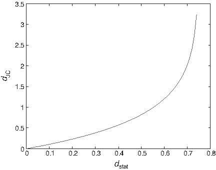
d_JC, as a function of d_stat.

A statistical model is currently applied to sequences in the Distance Matrix method (DM) or to characters as in the Maximum Likelihood method (ML). Now we apply the JC69-model to the probability representation model so that for two probability vectors p and q, Equation (9) becomes \documentclass{aastex}\usepackage{amsbsy}\usepackage{amsfonts}\usepackage{amssymb}\usepackage{bm}\usepackage{mathrsfs}\usepackage{pifont}\usepackage{stmaryrd}\usepackage{textcomp}\usepackage{portland,xspace}\usepackage{amsmath,amsxtra}\pagestyle{empty}\DeclareMathSizes{10}{9}{7}{6} \begin{document} \begin{align} d_ { JC } ( { \bf p } , { \bf q } ) = - \frac { 3 } { 4 } \ln \left( 1 - \frac { 4d_ { \rm stat } ( { \bf p } , { \bf q } ) } { 3 } \right) = - \frac { 3 } { 4 } \ln \left( 1 - \frac { 2 \ell_1 ( { \bf p } , { \bf q } ) } { 3 } \right). \tag { 10 } \end{align} \end{document}

Using this corrected statistical distance d_JC the MP approach for inferring probability phylogenetic trees becomes a problem asking for a probability Steiner tree T spanning a given set of probability matrices such that the total tree length \documentclass{aastex}\usepackage{amsbsy}\usepackage{amsfonts}\usepackage{amssymb}\usepackage{bm}\usepackage{mathrsfs}\usepackage{pifont}\usepackage{stmaryrd}\usepackage{textcomp}\usepackage{portland,xspace}\usepackage{amsmath,amsxtra}\pagestyle{empty}\DeclareMathSizes{10}{9}{7}{6} \begin{document} \begin{align} L ( T ) = \sum_ { { \bf P } { \bf Q } \in E } \left( \sum_ { k\ =\ 1 } ^m d_ { JC } ( { \bf p } ^ { k } , { \bf q } ^ { k } ) \right) = \sum_ { { \bf P } { \bf Q } \in E } \ \sum_ { k\ =\ 1 } ^m \left( - \frac { 3 } { 4 } \ln \left( 1 - \frac { 2 } { 3 } \sum_ { j\ =\ 1 } ^4 \mid p_j^k - q_j^k \mid \right) \right) \tag { 11 } \end{align} \end{document}

is minimized.

Theorem 3.1.

d_JC is convex.

Proof. The theorem is easily proved by the convex/concave rules for composition of functions (Boyd et al., 2004), however here we give a direct proof. Because the sum of convex functions is convex we need only to prove that d_JC(s, p) is a convex function of s with respect to any given p. That is, we need to show that for any two vectors s¹, s² \documentclass{aastex}\usepackage{amsbsy}\usepackage{amsfonts}\usepackage{amssymb}\usepackage{bm}\usepackage{mathrsfs}\usepackage{pifont}\usepackage{stmaryrd}\usepackage{textcomp}\usepackage{portland,xspace}\usepackage{amsmath,amsxtra}\pagestyle{empty}\DeclareMathSizes{10}{9}{7}{6} \begin{document} \begin{align} \frac { d_ { JC } ( { \bf s } ^1 , { \bf p } ) + d_ { JC } ( { \bf s } ^2 , { \bf p } ) } { 2 } \ge d_ { JC } \left( \left( \frac { { \bf s } ^1 + { \bf s } ^2 } { 2 } \right) , { \bf p } \right) , \end{align} \end{document}

This is equivalent to prove \documentclass{aastex}\usepackage{amsbsy}\usepackage{amsfonts}\usepackage{amssymb}\usepackage{bm}\usepackage{mathrsfs}\usepackage{pifont}\usepackage{stmaryrd}\usepackage{textcomp}\usepackage{portland,xspace}\usepackage{amsmath,amsxtra}\pagestyle{empty}\DeclareMathSizes{10}{9}{7}{6} \begin{document} \begin{align} 2 \ln \left( 1 - \frac { 2 } { 3 } \ell_1 \left( \frac { { \bf s } ^1 + { \bf s } ^2 } { 2 } , { \bf p } \right) \right) \ge \ln \left( 1 - \frac { 2 } { 3 } \ell_1 \left( { \bf s } ^1 , { \bf p } \right) \right) + \ln \left( 1 - \frac { 2 } { 3 } \ell_1 \left( { \bf s } ^2 , { \bf p } \right) \right) , \end{align} \end{document}

or \documentclass{aastex}\usepackage{amsbsy}\usepackage{amsfonts}\usepackage{amssymb}\usepackage{bm}\usepackage{mathrsfs}\usepackage{pifont}\usepackage{stmaryrd}\usepackage{textcomp}\usepackage{portland,xspace}\usepackage{amsmath,amsxtra}\pagestyle{empty}\DeclareMathSizes{10}{9}{7}{6} \begin{document} \begin{align} \left( 1 - \frac { 2 } { 3 } \ell_1 \left( \frac { { \bf s } ^1 + { \bf s } ^2 } { 2 } , { \bf p } \right) \right) ^2 - \left( 1 - \frac { 2 } { 3 } \ell_1 \left( { \bf s } ^1 , { \bf p } \right) \right) \left( 1 - \frac { 2 } { 3 } \ell_1 \left( { \bf s } ^2 , { \bf p } \right) \right) \ge 0. \tag { 12 } \end{align} \end{document}

Because ℓ₁ is convex, \documentclass{aastex}\usepackage{amsbsy}\usepackage{amsfonts}\usepackage{amssymb}\usepackage{bm}\usepackage{mathrsfs}\usepackage{pifont}\usepackage{stmaryrd}\usepackage{textcomp}\usepackage{portland,xspace}\usepackage{amsmath,amsxtra}\pagestyle{empty}\DeclareMathSizes{10}{9}{7}{6} \begin{document} \begin{align} 2 \ell_1 \left( \frac { { \bf s } ^1 + { \bf s } ^2 } { 2 } , { \bf p } \right) \le \ell_1 ( { \bf s } ^1 , { \bf p } ) + \ell_1 ( { \bf s } ^2 , { \bf p } ) , \end{align} \end{document}

Hence the left side of Equation (12) is \documentclass{aastex}\usepackage{amsbsy}\usepackage{amsfonts}\usepackage{amssymb}\usepackage{bm}\usepackage{mathrsfs}\usepackage{pifont}\usepackage{stmaryrd}\usepackage{textcomp}\usepackage{portland,xspace}\usepackage{amsmath,amsxtra}\pagestyle{empty}\DeclareMathSizes{10}{9}{7}{6} \begin{document} \begin{align} & \ge \left( 1 - \frac { 1 } { 3 } \ell_1 \left( { \bf s } ^1 , { \bf p } \right) - \frac { 1 } { 3 } \ell_1 \left( { \bf s } ^2 , { \bf p } \right) \right) ^2 - \left( 1 - \frac { 2 } { 3 } \ell_1 \left( { \bf s } ^1 , { \bf p } \right) \right) \left( 1 - \frac { 2 } { 3 } \ell_1 \left( { \bf s } ^2 , { \bf p } \right) \right) \\ & = \frac { \left( \ell_1 \left( { \bf s } ^1 , { \bf p } \right) - \ell_1 \left( { \bf s } ^2 , { \bf p } \right) \right) ^2 } { 9 } \ge 0. \end{align} \end{document}

The theorem is proved.

By this theorem L(T) in Equation (11) is convex and the phylogenetic tree problem for a given topology becomes a convex optimisation problem. Therefore we can use a convex optimisation program, say CVX (Grant et al., 2009), to solve it. Here we must point out that d_JC is not a real metric in a mathematical sense because it does not satisfy the Triangle Inequality. But the above formulation of the phylogenetic tree problem does make sense because the following theorem holds.

Theorem 3.2.

The set of feasible solutions of the Steiner points in T under the JC69-distance is not empty.

Proof. Because T is constructed site by site we need only consider a site, say site k. Moreover, because T is a tree, all nodes in T can be partitioned into two disjoint subsets U and V such that no two neighboring points lie in the same subset. It follows that we need only prove the existence of a Steiner point joining three terminals, say p, q and r. Let s^c = (p + q + r)/3 be the centroid of the triangle pqr. Then, by Theorem 2.2 we have 0 < 1 − 4d_stat(s^c)/3 < 1 and d_JC(p, s^c) > 0. Similarly, we have d_JC(q, s^c) > 0,d_JC(r, s^c) > 0. The theorem is proved.

Let s_JC(p, q, r) denote the optimal Steiner point for three terminals p, q and r. Then s_JC(p, q, r) does not necessarily lie in the plane \documentclass{aastex}\usepackage{amsbsy}\usepackage{amsfonts}\usepackage{amssymb}\usepackage{bm}\usepackage{mathrsfs}\usepackage{pifont}\usepackage{stmaryrd}\usepackage{textcomp}\usepackage{portland,xspace}\usepackage{amsmath,amsxtra}\pagestyle{empty}\DeclareMathSizes{10}{9}{7}{6} \begin{document} \begin{align} { \cal P} \end{align} \end{document} containing Δpqr. In general, the optimal Steiner point lies in a 3-dimensional unit cube. The probability points lying in the plane \documentclass{aastex}\usepackage{amsbsy}\usepackage{amsfonts}\usepackage{amssymb}\usepackage{bm}\usepackage{mathrsfs}\usepackage{pifont}\usepackage{stmaryrd}\usepackage{textcomp}\usepackage{portland,xspace}\usepackage{amsmath,amsxtra}\pagestyle{empty}\DeclareMathSizes{10}{9}{7}{6} \begin{document} \begin{align} { \cal P} \end{align} \end{document} can be expressed as p + x(q − p) + y(r − p) and lie within Δpqr if x ≥ 0, y ≥ 0, x + y ≤ 1. Then we can show that s^c in the proof of Theorem 3.2 is \documentclass{aastex}\usepackage{amsbsy}\usepackage{amsfonts}\usepackage{amssymb}\usepackage{bm}\usepackage{mathrsfs}\usepackage{pifont}\usepackage{stmaryrd}\usepackage{textcomp}\usepackage{portland,xspace}\usepackage{amsmath,amsxtra}\pagestyle{empty}\DeclareMathSizes{10}{9}{7}{6} \begin{document} \begin{align} { \bf s } ^c ( { \bf p } , { \bf q } , { \bf r } ) = \frac { { \bf p } + { \bf q } + { \bf r } } { 3 } = { \bf p } + \frac { 1 } { 3 } ( { \bf q } - { \bf p } ) + \frac { 1 } { 3 } ( { \bf r } - { \bf p } ). \end{align} \end{document}

Let s^p(p, q, r) denote the Steiner point in \documentclass{aastex}\usepackage{amsbsy}\usepackage{amsfonts}\usepackage{amssymb}\usepackage{bm}\usepackage{mathrsfs}\usepackage{pifont}\usepackage{stmaryrd}\usepackage{textcomp}\usepackage{portland,xspace}\usepackage{amsmath,amsxtra}\pagestyle{empty}\DeclareMathSizes{10}{9}{7}{6} \begin{document} \begin{align} { \cal P} \end{align} \end{document} that minimizes L(T) using the JC69-distance where T is the probability Steiner minimal tree on Δpqr. The difference between s^c(p, q, r), s^p(p, q, r) and s_JC(p, q, r) can be demonstrated in an example and the corresponding tree lengths are listed in Table 1.

Table 1.
Difference between s^c,s^p, and s_JC

Steiner point L(T)

s^c(p, q, r) [0.2043, 0.1684, 0.2553, 0.3721] 0.5664

s^p(p, q, r) [0.2237, 0.1551, 0.2274, 0.3938] 0.5138

s_JC(p, q, r) [0.2325, 0.1463, 0.2274, 0.3938] 0.5031

Let \documentclass{aastex}\usepackage{amsbsy}\usepackage{amsfonts}\usepackage{amssymb}\usepackage{bm}\usepackage{mathrsfs}\usepackage{pifont}\usepackage{stmaryrd}\usepackage{textcomp}\usepackage{portland,xspace}\usepackage{amsmath,amsxtra}\pagestyle{empty}\DeclareMathSizes{10}{9}{7}{6} \begin{document} \begin{align} { \bf p} & = [ 0.1079310237 , 0.1141927243 , 0.3840690551 , 0.3938071968 ] , \\ { \bf q} & = [ 0.2324521477 , 0.3057481166 , 0.2274139954 , 0.2343857403 ] , \\ { \bf r} & = [ 0.2724901539 , 0.08512508441 , 0.1542873004 , 0.4880974609 ] , \end{align} \end{document}

be three randomly generated probability vectors. Then the tree length L(T) with respect to the Steiner points in Δpqr is shown in Figure 2.

FIG. 2.
L(T) with respect to the Steiner points p + x(q − p) + y(r − p) in Δpqr.

4. Two Examples

Example 1.

Below is a simple example that consists of 5 sequences of 42 nucleotides (Felsenstein, 2009).
Turkey AAGCTNGGGC ATTTCAGGGT GAGCCCGGGC AATACAGGGT AT

Salmo gair AAGCCTTGGC AGTGCAGGGT GAGCCGTGGC CGGGCACGGT AT

H. Sapiens ACCGGTTGGC CGTTCAGGGT ACAGGTTGGC CGTTCAGGGT AA

Chimp AAACCCTTGC CGTTACGCTT AAACCGAGGC CGGGACACTC AT

Gorilla AAACCCTTGC CGGTACGCTT AAACCATTGC CGGTACGCTT AA

Note that there is an uncertain character “N” on site 6 in the sequence of Turkey, therefore in the probability representation model the input sequences on site six, [NTTCC]^T, will be represented by a 5 × 4 probability matrix \documentclass{aastex}\usepackage{amsbsy}\usepackage{amsfonts}\usepackage{amssymb}\usepackage{bm}\usepackage{mathrsfs}\usepackage{pifont}\usepackage{stmaryrd}\usepackage{textcomp}\usepackage{portland,xspace}\usepackage{amsmath,amsxtra}\pagestyle{empty}\DeclareMathSizes{10}{9}{7}{6} \begin{document} \begin{align} """\left( \begin{matrix}0.25 & 0.25 & 0.25 & 0.25 \\ 0 & 0 & 0 & 1 \\ 0 & 0 & 0 & 1 \\ 0 & 1 & 0 & 0 \\ 0 & 1 & 0 & 0\end{matrix} \right). \end{align} \end{document}

Let T_MP be the classical phylogenetic tree inferred by the classical MP method (e.g., Fitch's algorithm) (Fitch, 1971; Swofford et al., 1996), and T_p and T_JC be the optimal probability phylogenetic trees inferred using the standard statistical distance and JC69-distance respectively. First we should explain the difference caused by the different treatments of the character “N” in the classical MP method and in the probability representation model. In inferring T_MP using the classical MP method the character “N” is treated as a “wild card,” therefore, no substitution is incurred when “N” is compared with any other nucleotide character. However, as stated above, in the probability representation model ‘N’ is a probability vector with equal distributions at each component. As a result, L(T_p) = 44.7497 is larger than L(T_MP) = 44.

Remark 4.1.

As a comparison, assume that the character on site 6 in Turkey is not “N” but a gap “-.” Because in the classical MP method a gap is regarded as a 5th character different from A, C, G, T, and treated as neither A, nor C, nor G, nor T, one substitution is definitely incurred and the tree length T_MP would become 45.

The two probability phylogenetic trees T_p and T_JC are shown in Figure 3. From the picture it is clearly seen that L(T_JC) is much larger than L(T_p) (is about the double of L(T_p)). This is because the unobservable changes of nucleotides are taken into account in T_JC but are not in T_p.

FIG. 3.
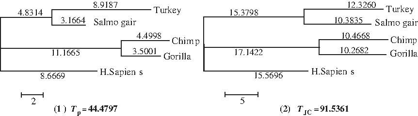
Two probability phylogenetic trees of Example 1.

Example 2.

This is a real example: The given set N containing 14 species is a part of a group of 25 species, originally studied in (Stanhope et al., 1996). The 14 sequences in N, listed in the Appendix, are 532 nucleotides long. Four different probability phylogenetic trees on N are shown in Figure 4 and the differences between the four probability phylogenetic trees are summarized in Table 2.
T₁: The tree is inferred by the MP method using the statistical distance dstat. Because there are no ambiguous characters in the input sequences its topology topo_MP and the tree length L(T₁) = 731 is the same as the optimal phylogenetic tree reconstructed by a classical MP method (Weng et al., 2008).

T₂: The tree is inferred with the same topology as T₁ but the length function is the JC69-distance d_JC. Note that, as in Example 1, we can see again that L(T₂) = 1428.66, is much larger than L(T₁) = 731 and L(T₂)/L(T₁) ≈ 2.

T₃: As mentioned above the Distance Matrix methods such as Neighbor Joining (NJ) can use substitution models to estimate unobservable substitutions. Let topo_NJ+JC denote the topology of the classical phylogenetic tree that is inferred by NJ using the JC69-model. Then T₃ is the probability phylogenetic tree that is inferred using JC69-distance with the topology topo_NJ+JC. L(T₃) = 1424.66, smaller than L(T₂).

T₄: Whether a tree is globally optimal or not depends on its topology. For this reason, T₃ is not the optimal probability phylogenetic tree because T₄ has a better topology and L(T₄) = 1424.55, a little smaller than L(T₃). In this example we didn't search the whole topology space of probability phylogenetic trees, hence, the topology of T₄ is possibly only sub-optimal, and denoted by topo_subopt.

FIG. 4.
Four probability phylogenetic trees of Example 2.

Table 2.
Comparison of Four Probability Phylogenetic Trees

Topology Distance Tree length

T ₁ topo_MP dstat 731

T ₂ topo_MP d_JC 1428.66

T ₃ topo_NJ+JC d_JC 1424.66

T ₄ topo_subopt d_JC 1424.55

5. Conclusion

We have laid out a new approach to the reconstruction of phylogenetic trees that combines the probability representation model with a substitution model. From the demonstrated examples, we can see that the probability representation model gives a solution to the puzzle of ambiguity and non-uniqueness in the reconstruction of phylogenetic trees. This probability representation model, which includes a substitution model, yields topologies, edge lengths, and ancestor states that are more likely to represent real biological evolution than that where no substitution model is used.

6. Appendix

Fourteen species of mammals

1. Marsupial Mole

GCTCCAGCAAATGATCAAGTACCAGGTATTGGAGGGCAATGTGGGTTACCTAAGAGTGGACTACATCCCTGGCCAG GAGGTAGTAGAAAAAGTCGGGGAGTTCCTGGTGAATGACATCTGGAAGAAGCTCATGGGGACATCCTCTCTAGTGC TAGATCTCCAGCACAGCACAGGGGGTGAAGTTTCGGGAATCCCCTTTGTCATTTCCTATCTACATCAGGGGGATAT CCTGCTCCATGTAGACACAGTTTATGACCGGCCATCAAACACTACCACAGAGATCTGGACCCAGCCTCAGGTGCTG GGTGAGAGGTATGGAGGGGAGAAGGACATGGTGGTTCTCACCAGCCATCATACTGTAGGGGTAGCTGAGGATATCG CCTATATTCTCAAGAAGATGCGCCGGGCCATTGTGGTGGGAGAGCAGACTCTGGGAGGGGCCCTAGATCTCCGGAA GCTGCGCATCGGTCAGTCAGACTTTTTCATCACTGTGCCCGTGTCACGCTCCCTGAGCCCCCTTGGTGGGGGGAGT

2. Wombat

GCTCCAGCAAATGATCAAGTACCAGGTACTGGAGGGTAATGTGGGTTACCTGAGAGTGGACTACATCCCTGGCCAG GAGGTGGTAGAGAAAGTCGGGGAGTTCCTGGTGAATGATGTCTGGAAGAAGCTCATGGGGACCTCTTCTCTGGTGT TGGATCTCCAGCACAGCACGGGAGGCGAAGTTTCAGGAATCCCGTTTGTCATTTCCTACCTACACCAGGGGGATAA TCTGCTGCATGTAGACACAGTTTATGACCGGCCATCAAACACCACCACAGAGATCTGGACCCTGCCCCAGGTGTTG GGTGAGAGGTACGGTGGGGAGAAGGACGTGGTGGTCCTCACCAGCCATCACACGGTCGGGGTAGCAGAGGATATTG CCTACATCCTCAAGAAGATGCGCCGGGCCATTGTGGTGGGAGAGCAGACTCTGGGAGGGGCCCTAGATCTCCGGAA GCTTCGTATTGGTCAGTCAGACTTTTTCATCACTGTGCCCGTGTCCCGTTCTCTGAGCCCCCTCAGTGGGGGGAGC

3. Rodent

GCTACAGAGGAATATTCACCATGAGGTTCTGGAGGGCAACTTGGGTTACCTATGGGTGGACGATCTCTTGGGCCAG GAGGTACTGAGTAAGCTCGGGGGATTCCTGGTGGCCCACATGTGGGGGCAGCTCATGAATACCTCTGGCTTGGTGC TAGATCTCCGGCACTGTACTGGGGGGCATGTTTCTGGTATTCCCTATGTCATCTCCTACTTGCACCCCGGGAACAC AATCATGCATGTGAACACCATCTATGATCGGCCCTCTAATACCACCACAGAGATCTGGACCTTGGCCAAGGTCCTG GGGGAGAGGTACAGTGCTGACAAGGATGTGGTGGTCCTCACCAGTGGCCACACTGGAGGAGTGGGTGAGGACATTG CCTATATCCTCAAACAGATGCGCAGGGCCATCATGGTGGGTGAGCAGACTGAAGGTGGTGCCCTGGACCTCCAGAA ACTGAGGATAGGCCAGTCCAACTTCTTCCTCACAGTGCCTCTGGCGATGTCTCTGGGGCCGATGGGTGGAGGTGGC

4. Elephant Shrew

GCTGGAGAGAAGCATGAGCTACAGGATTCTGGATGGTAATGTGGGCTACTTGCAGATAGACAACATCCCAGGCCAG GAGGTACTGAGCCGACTAGGGGCCTTCCTGGTGGCCCATGTCTGGAGACAGCTCATGGGCACCTCTGCTTTGGTGT TGGACCTGCGGCAGTGCACAGGAGGCCATGTTTCCAGCATCCCTTACCTTATTTCCTACCTGCACCCAGCGGGCAC GGTCCTGCACGTTGACACCATTTACAACCGTCCCTCTAACACAACCACTGAGCTCTGGACTTTGCCTCAGGTGCTT GGGGAGAGATACAGTGCTGAGAAGGATGTGGTGGTCCTCACCAGTGGTCAAACCCGGGGTGTGGCTGAGGACATTG TCTACATCCTCAAGCAGATGGGCAGGGCCATAGTGGTGGGTGAACGTACTGGGGGGGTCTCCCTGGACCTCCAGAA GCTAAGGATAGCCAACTCTGACTTCTTCCTCACTCTACCTGTGTCCAGGTCCTTGGGGCCTCTGGGTGGAGGCACC

5. Elephant

GCTGCAGACAAGCATGAGCTACAAGGTTCTGGAGGGCAACGTGGGCTACCTGCGGGTAGACAACATCCCAGGCCAG GAGGTGCTGAACCAGCTGGGGGCCTTCCTGGTGACTCACGTCTGGAAGCAGCTTATGGGCTCCTCTGCCTTAGTGC TGGACCTGCGACACTGCACAGGGGGCCATGTCTCCAGCATCCCTTACCTCATTTCCTACCTGCACCCGGGCGGCAC CGTGCTGCACGTGGACACCATTTACAACCGCCCCTCCAATACGACTACGGAGCTCTGGACCTTGCCCCAGGTGCTG GGGGAGAGGTATAGCGCCGACAAGGATGTGGTGGTCCTCACCAGTGGCCACACCAGGGGCGTGGCCGAGGACATCG TCTACATCCTCAAGCAGATGGGCAGGGCCATCGTGGTGGGCGAGCGGACTGAGGGTGGTGCCCTGGACCTCCAGAA GATAGGCCACTCTGACTTCTTCCTCACTCTGCCTGTGTCTAGGTCCTTAGGCCCCCTGGGCGGGGGAAGCCAGACA

6. Whale

GCTGCAGAACGGCCTCCGCCATGAGGTTCTGGAAGGCAATGTGGGCTACCTGCGGGTGGACGACATCCCAGGCCAG GAGGTGATGAGCAAGCTGAGGAGCTTCCTGGTGGCCAACGTCTGGAGGAAGCTCATGGGCACCTCTGCCTTGGTGC TGGACCTCCGCCATTGCACTGGGGGCCACATTTCTGGCATCCCCTATGTCATCTCCTACCTGCACCCGGGGAACAC AGTCCTGCACGTGGATACCATCTATGATCGCCCCTCTAATACGACCACTGAGATCTGGACCCTGCCCGAAGTCCTA GGAGAGAACTACGGTGCCGATAAGGATGTGGTGGTCCTCACCAGTGGTCGCACCGGGGGTGTGGCTGAGGACATCG CTTATATCCTCAAACAAATGCGCAGGGCCATTGTGGTGGGCGAGCGGACTGTGGGGGGGGCCTTGGACCTCCAGAA GATAGGCCAGTCTGACTTCTTTCTCACCGTGCCCGTGTCCAGGTCCCTGGGGCCCCTGGGCAAGGGCAGTCAGACT

7. Dolphin

GCTGCAGAACGGCTTCCGCCATGAGGTTCTGGAAGGCAATGTGGGCTACCTGCGGGTGGACGACATCCCGGGCCAG GAGGTGATGAGCAAGCTGAGGAGCTTCCTGGCGGCCAACGTCTGGAGGAAGCTCATGGGCACCTCTGCCTTGGTGC TGGACCTCCGCCACTGCACTGGCGGCCACATTTCCGGCATCCCCTATGTCATCTCCTACCTGCACCCAGGGAACAC AGTCCTGCATGTGGATACCATCTACGATCGCCCCTCTAATACGACCACTGAGATCTGGACCCTCCCCGAAGTCCTA GGAGACAACTACGGTGCCGATAAGGATGTGGTGGTCCTCACCAGTGGTCGCACGGGGGGTGTGGCTGAGGACATCT CTTATATCCTCAAACAGATGGACAGGGCCATCGTGGTGGACGAACGGACTGTGGGGGGGGCCTTGGACCTCCAGAA GATAGGCCAGTCTGAGTTCTTTCTCACAGTGCCCGTGTCCAGGTCCCTGGGGCCCCTGGGCAAGGGCAGCCAGACT

8. Pig

GCTGCACAATAGTCTCCGCCATGAGGTTCTGGAAGGCAATGTGGGCTACCTGCGGGTGGACGACATCCCAGGCCAG GAGGTGATGAACAAGCTGGGGAGCTTCCTGGTAGTCAACGTCTGGGAAAAGCTAATGGGCACCTCTGCCTTGGTGC TAGACCTCCGGCACTGCACCAGGGGCCACGTTTCTGGCATCCCCTATGTCATCTCCTACCTGCACCCAGGGAACAC GGTCCTGCACGTGGACACCATCTATGACCGTCCCTCCAATACGACCACTGAGATCTGGACCCTGCCCGAAGTCCTG GGAGACAGGTACAGTGCGGATAAGGACGTGGTGGTCCTCACCAGCAGCCACACAGGGGGCGTGGCTGAGGACATCG CCTACATCCTCAAACAGATGCGCAGGGCCATTGTGGTCGGCGAGCGAACTGTGGGGGGTGCCCTGGACCTCCAGAA GATAGGCCAGTCCGACTTCTTTCTCACCGTGCCTGTGTCCAGGTCCCTGGGGCCCCTGGGTGAGGGCAGCCAGACA

9. Horse

GCTGCAGGAGGGCATCCGCTATGACATTCTGGAGGGCGACGTGGGCTACTTGCGAGTGGACAACATCCCGGGCCAG GAGGTGGTGAGCAAGCTGGGGGGCTTCCTGGTGGACAATGTCTGGAGGAAGCTCATGGGCACCTCTGCCTTGGTGC TGGACCTCCGGCACTGCACTGGGGGCCACGTTTCCGGCATCCCCTATATCATCTCCTACCTGCACCCAGGAAACAC GGTCCTGCACGTGGACACCATCTACGACCGCCCCTCCAATACGACCACTGAGATCTGGACCCTGCCCGAGGTCCTG GGAGAGAGGTACAGTGCCGACAGGGATGTGGTGGTCCTCACCAGTGGCCACACCGGGGGCGTGGCCGAGGACATTG CTTACATCCTCAAACAGATGCGCAGGACCATCGTGGTGGGTGAGCGGACCGTGGGAGGTGCCCTGGACCTCCAGAA GATAGGCCAGTCCGACTTCTTCCTCACCGTGCCCGTGTCCAGGTCCCTGGGTCTGCGCGAGGTCCTCATGCATAAC

10. Bat

GCTGCAAAAGGCCATCCACTACAATGTTCTGGAGGGCAACGTGGGCTACTTTCGGGTGGACGACATCCCGAGCCAG GAGGTGGTGAGCAATCTTGGGGGCTTCCTCGTGGACAATTTCTGGAGGAAGCTCCTGGGCACCTCTGCCTTGGTGC TAGACCTCCCACACTGCACTGGGGGGCACGTTTCTGGGATCTCCTATGTCATCTCCTACTTGCACCGAGGGAACAC CGTCCTGAATGTGGACCCACTCTATGACCCCCCCTCCAACACGACCACAGAGATCTGGACCCTGCCCCAGGTCCTG GGAGAGAGGTACAGTGCTGACAAGGATGTTGTGGTCCTCACCAGTGGCCACACTGGAGGAGTGGCTGAGGACATTG CTTACATCCTCAAACAGATGCGCAGGGCCATTGTGGTGGGTGAGCAGACTGTGGGGGGTGCCCTGGACCTCCAGAA GATAGGCCAGTCTGACTTCTTCCTCACTGTGCCTGTGTC TAGGTCCCTGGGGGCTCTGGGTGGGGGCAGGCAGACA

11. Insectivore

GCTGCAGAGGGCCATCCGCTACCAGGTTCTGGCGGCCAATGTGGGCTACCTGGGGAGGGATAACCTCCCCGGTCAG GAGGTGGTGACCATACTGGGGGCTCTCCTGGTGGCCAATGTCTGGGGGAAGCTCATAGCCACCTCTCCCTTGGTGC TGGACCTCCGACACTGCACTGGGGGCCATGTCTCTGGGATCCCCTACGTCATCTCCTACCTGTACCCAGGAAACAC GGTCCTGCATATGGACACCATCTATGACCGCCCCTCCAATATCACCACTGAGCTCTGGACCCTGCCCCAGCTCCAG GGAGAGCGGTACGGTGCAGACAAGGATGTGGTGGTCCTCATCAGCGACCACACTGGGGGTGTGGCTGAGGACATTA CTTACATCCTCAAACAGATGCGCCGGGCTATTGTGGTGGGCGAGCAGACTGTGGGGGCTGCTCTGGACCTCCAGAA GATAGGCCAGTCTGACTTCTTCATCACTCTGCCTGTCTCCAGGTCTCTGGGGACTCTGGGCGGGGGCAGCCAGACA

12. Human

GCTGCAAAGGGGCCTCCGCCATGAGGTTCTGGAGGGTAATGTGGGCTACCTGCGGGTGGACAGCGTCCCGGGCCAG GAGGTGCTGAGCATGATGGGGGAGTTCCTGGTGGCCCACGTGTGGGGGAATCTCATGGGCACCTCCGCCTTAGTGC TGGATCTCCGGCACTGCACAGGAGGCCAGGTCTCTGGCATTCCCTACATCATCTCCTACCTGCACCCAGGGAACAC CATCCTGCACGTGGACACTATCTACAACCGCCCCTCCAACACCACCACGGAGATCTGGACCTTGCCCCAGGTCCTG GGAGAAAGGTACGGTGCCGACAAGGATGTGGTGGTCCTCACCAGCAGCCAGACCAGGGGCGTGGCCGAGGACATCG CGCACATCCTTAAGCAGATGCGCAGGGCCATCGTGGTGGGCGAGCGGACTGGGGGAGGGGCCCTGGACCTCCGGAA GATAGGCGAGTCTGACTTCTTCTTCACGGTGCCCGTGTCCAGGTCCCTGGGGCCCCTTGGTGGAGGCAGCCAGACG

13. Sea Cow

GCTGCAGACCAGCATGAGCTACAAGGTTCTGGATGGCAATGTGGGCTACCTGCGGGTAGACAACATCCCTGGCCAG GAGGTGCTGAGCCGTCTGGGGGGCTTCCTGGTGACTCACATCTGGAAGCAGCTCATGGGCTCCTCTGCCTTAGTCC TGGACCTGCGGCACTGTATGGGTGGCCATGTCTCCAGCATCCCTTACATCATCTCCTACCTACACCCCGGAGGAGC AGTGCTGCATGTGGACACCATTTACAACCGCCCCTCCAATACGACTACTGGGGTCTGGACCTTGCCCCAAGTGCTG GGAGAAAGGTACAGTCCCAACAAGGATGTGGTGGTCCTCACCAGTGGCCACACCAGGGGCGTGGCCGAAGACATCG TTCACATCCTTAAGCAGATGGGCAGGGCCATAGTGGTGGGCGAGAAGACGGAGGCAGGTGCCCTGCACCTCCAGAA GATAGGTCACTCTGATTTCTTTCTCACTCTGCCTGTGTCCAGGTCCTTGGGGCCTTTGGGCAGGGGAAGCCAGACA

14. Hyrax

ACTGCAGACAAGCATGAGCTACAAGGTTCTGGAGGGCAACGTGGGTTACCTGCGGGTAGACAACATTCCGGGTCAA GATGTGCTGAACCAGCTGGGGGGCTTCCTGGTGACTCATGTGTGGAAGCAGCTCATGGGCTCCTCTGCCTTAGTGC TGGACCTAAGGCACTGCACGGGGGGCCATGTCTCCAGTATCCCTTACCTCATCTCCTACCTGCATCCAGGGAGCAC TGTGCTGCACGTGGACACCATTTACAACCGCCCCTCCAATACAACTACTGAGCTCTGGACCTTGCCCCAGGTGCTG GGGGAGAGATACAGTGCTGACAAGGATGTGGTGGTCCTCACCATGGGCCACACCAGGGGTGTGGCCGAGGACATCG TCTACATCCTCAAGCAGATGGGCAGGGCCATTGTGGTAGGCGAGCGGACCGAGGGTGGTGCCCTGGACCTCCAGAA AATAGGTCACTCAGACTTCTTTTTCACTCTGCCTGTGTCCAGGTCACTGGGCCCCTTAGGCAGGGGAAGCCAGACA

	Steiner point	L(T)
s^c(p, q, r)	[0.2043, 0.1684, 0.2553, 0.3721]	0.5664
s^p(p, q, r)	[0.2237, 0.1551, 0.2274, 0.3938]	0.5138
s_JC(p, q, r)	[0.2325, 0.1463, 0.2274, 0.3938]	0.5031

	Topology	Distance	Tree length
T ₁	topo_MP	dstat	731
T ₂	topo_MP	d_JC	1428.66
T ₃	topo_NJ+JC	d_JC	1424.66
T ₄	topo_subopt	d_JC	1424.55

Footnotes

Disclosure Statement

No competing financial interests exist.

References

Althaus

, Naujoks

2006. Computing Steiner minimum trees in Hamming metric. Proc. SODA 06.

Boyd

, Vandenberghe

2004. Convex Optimization. Cambridge University Press: Cambridge, UK.

Brazil

, Thomas

D.A.

, Nielsen

B.K.

et al. 2009. A novel approach to phylogenetic trees: d-dimensional geometric Steiner trees. Network, 53:104–111.

Ewens

W.J.

, Grant

G.R.

2005. Statistical Methods in Bioinformatics: An Introduction. Springer: New York.

Felsenstein

2004. Inferring Phylogenetics. Sinauer Associates Inc.: Sunderland, MA.

Felsenstein

2009. Molecular sequence programs. http://evolution.genetics.washington.edu/phylip/doc/sequence.html. 2010 June 1.

Fitch

W.M.

1971. Toward defining the course of evolution: minimum changes for a specific tree topology. Syst. Zool., 20:406–416.

Foulds

L.R.

, Graham

R.L.

1982. The Steiner problem in phylogeny is NP-complete. Adv. Appl. Math, 3:43–49.

Grant

, Boyd

. 2009. CVX: Matlab software for disciplined convex programming [web page and software] http://stanford.edu/boyd/cvx. 2010 June 1.

10.

Galtier

, Gascuel

, Jean-Marie

2005. Markov models in molecular evolution, 3–24. Nielsen

Statistical Methods in Molecular Evolution. Springer: New York.

11.

Hwang

F.K.

, Richards

D.S.

, Winter

1992. The Steiner Tree Problem. Elsevier Science Publishers B.V.: Amsterdam.

12.

Jukes

T.H.

, Cantor

C.R.

1969. Evolution of protein molecules, 21–132. Munro

M.N.

Mammalian Protein Metabolism. Academic Press: New York.

13.

Liberti

, Maculan

2006. Global Optimization: From Theory to Implementation. Springer: New York.

14.

Liébecq

1992. Biochemical Nomenclature and Related Documents, 2nd. Portland Press: Portland, OR.

15.

Stanhope

M.J.

, Smith

M.R.

, Waddell

V.G.

et al. 1996. Mammalian evolution and the interphotoreceptor retinoid binding protein (IRBP) gene: convincing evidence for several superordinal clades. J. Mol. Evol., 43:83–92.

16.

Steel

, Penny

2000. Parsimony, likelihood, and the role of models in molecular phylogenetics. Mol. Biol. Evol., 17:839–850.

17.

Swofford

D.L.

, Olsen

G.J.

, Waddell

P.J.

et al. 1996. Phylogenetic inference, 407–514. Hilles

D.M.

, Moritz

, Mable

B.K.

Molecular Systematics, 2nd. Sinauer Associates: Sunderland, MA.

18.

Xia

2006. Molecular phylogenetics: mathematical framework and unsolved problems, 171–191. Bastolla

, Porto

, Roman

H.E.

et al. Structural Approaches to Sequence Evolution. Springer: New York.

19.

Weng

J.F.

, Mareels

, Thomas

D.A.

2008. Probability representation of ancestral states in phylogenetic trees. Proc. EURO-CBBM 2008. www.iasi.cnr.it/iasi/RomeConference/abstract_book.pdf. 2010 June 1.