Re-Evaluating the “Rules” of Protein Topology

Abstract

It is well known that the set of observed topological arrangements of secondary structures in globular proteins is highly limited. These limitations have been explained as the consequence of several rules of thumb including a strong preference for right-handed connections, against crossing loops and certain beta strand patterns. We present a critical evaluation of the power of these rules to distinguish known from possible topologies in a large set of two- and three-layer protein structures and determine that although these rules are still largely valid, an increasing number of exceptions can be found to many of them. The rules are then used to construct a generalised linear model for assessing the probability of occurrence of an arbitrary topology in the PDB. Application of the model to a large set of topologies generated during structure prediction showed that many had a similar probability of occurrence to known PDB folds. Supplementary Material is available online at www.liebertonline.com.

1. Introduction

1.1. Secondary structure lattice models

Simplified representations of protein structure have been widely used in both the analysis and prediction of protein structure for many years (Richardson, 1977; Ptitsyn and Finkelstein, 1980; Efimov, 1997. See also [Taylor and Aszódi, 2005], for a review). In general, the greater the degree of simplification, the easier it becomes to computationally explore variation in conformational degrees of freedom but this is countered by the loss of detail in the representation of the protein structure. The extent to which simplification can be tolerated depends on the nature of the problem being addressed. If the problem is enzyme active site catalyzis rate, then even the loss of hydrogen positions may be important, whereas looking at larger conformational changes (say, by normal mode analysis), the loss of side-chain positions can be tolerated. When the subject of interest is the overall fold of the protein chain then even an α-carbon representation (one point per amino acid) does not provide sufficient freedom to look at chain rearrangements in a reasonable time. A suitable level to analyze large chain rearrangements is to treat each secondary structure element (SSE) as a unit. This provides a degree of simplification of roughly an order of magnitude over the α-carbon level as each SSE of ten or more residues can be located by either one or two coordinate points. Two coordinates can be used for the end-points of each SSE giving a stick-like model, whereas one coordinate (say, the mid-point of each SSE line-segment) results in an almost 2-dimensional representation. If the SSE sticks are reasonably well aligned (or have an overall regular twist), then one of the three dimensions can be eliminated, providing the protein is not too large (say, under 20 SSEs) or has a regular overall twist.

These pseudo-2D1 representations can be slightly regularized without much loss of detail by fixing the coordinates on a regular grid, or secondary structure lattice, with a 5Å spacing between β-strands and double between all other SSEs. This regularized simple representation of a protein structure has been shown to be reasonable by the reconstruction of the full protein structure using the SSE-lattice coordinates as a starting point. Proteins up to almost 200 residues have been regenerated from their lattice fold specification resulting in models within 5Å RMSD of the native structure (Taylor et al., 2008, 2009) and additional refinement to main-chain level allows reasonable side-chain positions to be added (MacDonald et al., 2009).

1.2. Exhaustive fold enumeration

The regeneration of protein structrures from their secondary structure lattice specification implies that this very simple representation provides a valid tool to explore the conformational freedom of protein structures at the level of the chain fold. This exploration can be viewed in terms of an abstract fold-space in which distinct folds are embedded with the most similar folds lying adjacent (Orengo et al., 1993; Hou et al., 2003; Taylor, 2007). In this representation, features of the space can be investigated, such as how the number of folds depends on the starting configuration or how interconnected the space is. Two approaches to this exploration are possible: one would be to specify a set of edit and move operations for the SSEs over the lattice similar to those used in residue-level lattice simulations or to use vertex displacement over the discrete space of a polyhedron (Hinds and Levitt, 1992; Luo et al., 1993), and use these to stochastically explore the space starting from known points. Alternatively, since the proteins considered are relatively small and computers are relatively fast, it is possible to exhastively enumerate all possible arrangements of the given SSEs over a lattice.

Previous investigations in this direction have been made with a view to the elimination of secondary structure combinations that are rarely, if ever, seen in known protein structures with the hope that this will improve the chance of predicting a correct tertiary structure (Cohen et al., 1980; Woolfson et al., 1993; Ruczinski et al., 2002; Taylor et al., 2008). Typically, these investigations identified ad hoc “rules” that were valid given the then current range of structures seen in the protein databank. With the less ambiguous registration of strands in a sheet compared to α-helix-packing, most of these studies also focused on β-sheet topology. Although some of the early “rules” appear to remain valid over time, such as the avoidance of “pretzel” topologies (proposed by Cohen et al. and still seen to be avoided by Ruczinski et al. more than 20 years later), the reliability of others, such as the avoidance of cross-over connections (Cheng and Grishin, 2005) and even the hand of connection between strands in the sheet (Sternberg and Thornton, 1977; Hutchinson and Thornton, 1993) have increasing numbers of exceptions.

In this study we focus mainly on the two-layer protein architectures (βα and ββ), with some limited consderation of the three-layer αβα architecture. We do not consider proteins that contain a β-barrel or those with specialist arrangements (such as the β-propellor). It is also beyond the scope of our methods to analyse the all-α proteins as these do not have sufficiently well defined layers, however, polyhedral models may provide a route towards including this class (Murzin and Finkelstein, 1988). Our approach in this study is to accept the ad hoc source of the various topological rules that have accumulated over the years and to test them both singly and in combinations to evaluate their power at reducing the number of possible folds while eliminating as few known folds as possible. In this way, we can then develop a set of fold filters that may have some use in restricting the list of candidate folds for structure prediction or, if embedded in a fold generating function, of only generating folds which have a good chance of being correct.

2. Basic Methods and Preliminary Results

2.1. Protein data

To enumerate protein topologies we need to reduce the three dimensional structure to a string of text that contains the topological information about the connections of the secondary structure layouts. For this we adopted the method outlined in the introduction in which a protein structure is reduced to a simplified coordinate representation based on layers of secondary structures in which secondary structure elements (SSEs) are represented by line-segments in an idealised lattice (called an “Ideal Form”) (Taylor, 2002a). The resulting pseudo-2D representation corresponds directly to topology cartoons in which α-helices are represented by circles and β-strands by a square or triangle (Nagano, 1977; Sternberg and Thornton, 1977; Flores et al., 1994).

Each layer of secondary structures in the Ideal-form is labelled alphabetically, with the top and bottom alpha layers as “A” and “C” respectively and the top and bottom beta layers “B” and “E” respectively (or just “B” if there is only one β-sheet). The first element along the chain to enter each layer is labelled “+0” and the other elements in the layer are labelled relative to this, taking right as the positive direction. The orientation of each element is given by the sign proceeding the letter. See Figure 1 for an example.

FIG. 1.

Example of reduction from 3D structure (upper) to a 2D diagram (lower) and finally to the 1D string: +B+0.−A+0.+B−2.−B−1.+A+1.−B+1. The secondary structure layout, or architecture, is αα – ββββ.

Matches to the Ideal Forms were generated for all domains in the SCOP40 non-redundant database which is selected to exclude any pair of proteins with more than 40 percent sequence identity (Murzin et al., 1995). Of the 9,479 domains in the set 7,117 were found to have at least one form match. Matches were sorted by a score based on the packing between elements, endpoint RMSDs and a density term dependent on local structure (more fully described in [Taylor, 2002b]) and the best scoring form hit for each domain was retained. In total there were matches to 5,543 unique domains by three-layer forms and 1,600 to four-layer forms. No topology strings were generated for barrel forms. Since the relationship between form matches and domains can be many-to-one all matches were retained.

Each topology string resulting from an ideal form match was used to generate a series of subtopologies by deletion from the termini of the string (which are the same as the sequence termini), using the requirements of compactness and good packing to ensure that the deletions would not generate gaps in sheets or delete strands on either side of a helix without also deleting the helix. The strings generated were (typographically) rotated to ensure that no duplications or ambiguities were possible by ensuring that the first strand is in layer ‘B’ position 0 and the first helix is in layer ‘A’ position 0, (except where there were four strands, in which case the alpha-layering was defined by the position relative to the two beta layers). These rules are sufficient to resolve ambiguities except where there is only a single sheet, in which case the additional requirement was made that the second strand must be to the right of the first.

A program was written using the Perl module Math::Combinatorics to find all the possible topological structures a protein could adopt for each of several secondary structure layouts comprising: βββ – βββ, ββββ – ββββ, α – ββββ, αα – ββββ and ααα – ββββ (where a dash separates the number of SSEs in each of two layers). When calculating all possible topologies it was important to take account of symmetry in each layout to avoid double counting identical folds. The number of structures for each secondary structure layout are given in Table 1.

Table 1.

Frequencies of Topology Strings Meeting Conditions of the Seven Filters. Raw Hits (N Filter) and Proportions (Frac) Relative to all Substrings in Each Subset (N Tot) are Shown for Two Secondary Structure Layouts and All PDB Structures. Frequencies are Also Shown for Best-Match PDB Structures (Col 3) in Addition to Substrings (Col 4)

		Layout
		ββββ-ββββ (sub)			ααα-ββββ (sub)			All in PDB (full)			All in PDB (subtopols)
Filter		N (filter)	N (tot)	Frac	N (filter)	N (tot)	Frac	N (filter)	N (tot)	Frac	N (filter)	N (tot)	Frac
Parallel	P	21	311	0.067	833	2875	0.289	110	3003	0.140	90,256	223296	0.404
Non-Edge Parallel	E	3	311	0.001	172	2875	0.060	84	3003	0.027	43,266	223206	0.194
Crossover	C	33	311	0.106	269	2875	0.093	127	3003	0.042	17,767	223206	0.080
Left-hand Turn	L	79	311	0.254	423	2875	0.147	506	3003	0.168	27,881	223206	0.125
Layer Crossover	BC	2	311	0.001	1	2875	0.000	30	3003	0.010	1,582	223206	0.007
Clash	CL	2	311	0.001	56	2875	0.019	53	3003	0.028	15,436	223206	0.069
Pretzel	O	3	311	0.001	12	2875	0.004	8	3003	0.002	439	223206	0.002

2.2. Topological filters

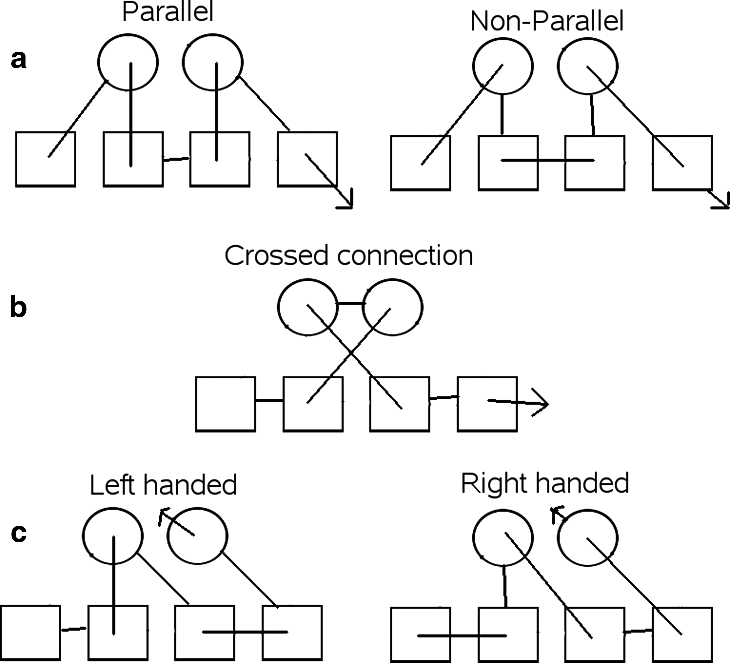
There are many rules which have been identified over the years which describe the way in which secondary structure elements can connect and pack with each other. Our aim is to encode and apply these rules to our unconstrained topologies (the full set). From the literature, we identified three main general filters that apply to the local configuration of a few SSEs:

Parallel connections are unfavorable: It can be argued that consecuitive parallel connections between SSEs are not favored because they leave more unsatisfied hydrogen-bonds compared to the, typically, shorter connections between adjacent ends. A supporting argument can also be found by considering chain entropy.2 (See Figure 2a for examples of parallel connections.)

Crossing connections are unfavorable: Connections between SSEs tend not cross because a crossover will bury some of the main chain. As the main-chain contains polar atoms, this will cause an increase in free energy (Woolfson et al., 1993). Alternatively, if the polar atoms are satisfied by pairing into hydrogen bonds then the buried chain segment will most likely be redefined as a secondary structure. (See Figure 2b for example of crossing connections.)

Left-handed connections are unfavorable: In our model, we define a left-handed connection between any two SSEs in a beta layer via a SSE in a different layer as unfavorable. Using equation (1), it can be shown that right-handed connections minimize the free energy of a protein structure (Finkelstein and Ptitsyn, 1987). We do not consider the chirality of parallel β-strands linked only by a loop as the topology strings do not specify whether a connecting loop passes above or below the β-sheet. (See Figure 2c for examples of left- and right-handed connections.)

FIG. 2.

Structure examples.

We eliminated folds with any of these undesirable characteristics for the αα – ββββ and the ββββ – ββββ secondary structure layouts initially. Removing strings with these characteristics from the full set of topologies yields a 99.9% reduction in the number of allowed folds for the ββββ – ββββ string and 98.8% for αα – ββββ. (Table 2).

Table 2.

Enumerations for Given Secondary Structure Layout after Structures with Crossing, Left-Handed and Parallel Connections Have Been Eliminated and Number of Times These Occur in the Known Structures

Secondary structure layout	% possible structures	% known structure hits
ββββ – ββββ	0.01	18.5
αα – ββββ	1.2	10.0

3. Results and Discussion

3.1. Filtering known structures

The large reductions in the number of topologies caused by applying the filters are only useful if they do not eliminate a significant proportion of known topologies. For this reason, we tested the filters on topology strings taken from Protein Data Bank (PDB) structures (Taylor et al., 2009). (Data included as Supplementary Material; see online at www.liebertonline.com)

For the ββββ – ββββ string 81.5% were eliminated and for the αα – ββββ string, only 90.0% were eliminated (Table 2). While large, these are lower percentages than those seen for the full set and confirms that loop crossing, left handed and parallel connections are quite unfavorable.

Examination of the known folds that failed to pass the filters revealed that many had parallel connections. Despite a clear bias for non-parallel connections (Table 3), this “preference” is not strong enough to justify the elimination of all structures with parallel connections. For example if we make the simple assumption that the connections are distributed randomly throughout the structures then by considering a binomial distribution we would expect to see at least one parallel connection in each structure for all the secondary structure layouts we are considering.

Table 3.

Number of Parallel and Non-Parallel Connections in Topologies Containing One and Two Layer Beta Sheets

Set of known structures	No. of non-parallel connections	No. of parallel connections
One layer β sheet	251276	83285
Two layer β sheet	248155	70612

The basic filters tested here have previously been evaluated by others (Finkelstein and Ptitsyn, 1987; Woolfson et al., 1993), with similar conclusions being drawn. However, a loss rate of 80–90% of valid folds would be quite unacceptable in a realistic structure prediction exercise and a less strict filtering strategy is clearly required.

3.2. Additional and revised filters

Taking a closer look at the structures with parallel connections revealed that the parallel connections mostly occur on the edge of the structure. For the ββββ – ββββ derived folds, only 22.6% have parallel connections not on an edge and 26.1% for αα – ββββ. This motivated us to change the filter that removes all structures with parallel connections to one that distinguishes between parallel on the edge and parallel connections through the middle of the structure.

Parallel connections within the same β-sheet can be left or right handed (Richardson, 1976). However, our topological model is unable to establish the handedness of these connection as it does not specify whether the connection will go above or below the sheet. To overcome this limitation we assumed that all parallel beta sheet connections are right handed. This assumption allows us to apply the clash filter defined by Ruczinski et al. (2002), which eliminates structures where parallel beta connections cross over. This filter is different from the previously mentioned crossover filter as the connections bridge ends of the same layer rather than different layers.

The “pretzel” is a filter used by Cohen et al. (1982), which eliminates structures based on the order in which the β-strands are connected within a sheet. If i,j,k,l are sequential strands in a sheet, then the filter eliminates structures where the strands occur in the following orders k,i,l,j and j,l,i,k. Another filter which is related to the “pretzel” filter eliminates structures where the connections between secondary structure elements in the same layer crossover (Ruczinski et al., 2002), we call this filter the “layer crossover.”

Another filter we tested checks the connections between elements in the same layers that jump over other SSEs (Woolfson et al., 1993; Ruczinski et al., 2002). Woolfson also mentions several filters that apply to beta sandwich structures (Woolfson et al., 1993), which can in principle be extended to αβ structures.

These revised and additional filters are itemized below specifying the configuration that they eliminate, along with the one or two letter memnonic that will be used to refer to them. Some are illustrated in Figure 3.

Layer crossover (BC): Crossovers between non-parallel beta sheet connections which do not pass through alpha helices on the sides of the structure.

Clash (CL): Crossover between parallel connections of any secondary structures on the top or bottom layer.

Pretzel (O): If i,j,k,l are sequential strands in a sheet, then the filter eliminates strings in which the strands occur in the following orders k,i,l,j and j,l,i,k.

Left-handed connection (L): Left-handed beta-alpha-beta and beta-beta-beta connections.

Crossover (C): Crossover between the non-parallel connections between secondary stucture elements which pass through the center of the structure.

Jump (M with following number): The number after the M sets the maximum cumulative jumps over elements in a given layer without passing through another layer.

Parallel count (E with following number): This filter eliminates topologies with a number of non-edge parallel connections, 0 permits only edge parallel connections, 1 permits a single non-edge parallel connection.

FIG. 3.

Examples of topological filters described in the text are depicted on a two-layer αβ layout. Each filter is identified by a code that corresponds to the list of filters in the text.

3.3. Evaluation of the individual filters

Figure 4 displays several graphs illustrating how well each filter performs when measured by the relative numbers of known folds that pass the filters and the number eliminated from the full set.

FIG. 4.

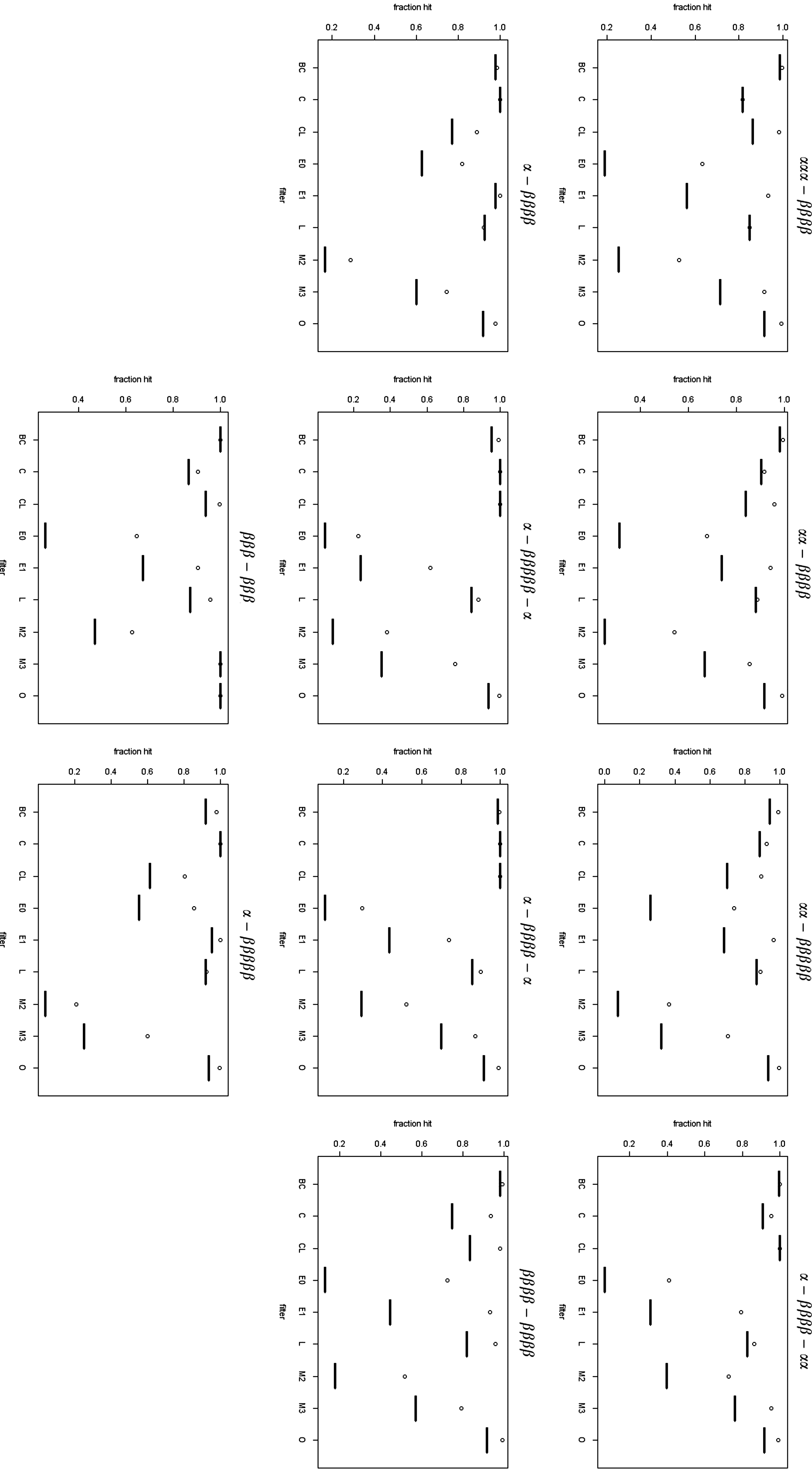
For each secondary structure layout the black bar represents the proportion of the full set remaining after the filter and the white dot represents the proportion of the known structures remaining after the filter. Key to filters: O, pretzel; CL, clash; BC, beta crossover; C, crossver; M, jump; E, non-edge parallel connection; L, left-handed connection.

Layer crossover (BC) performs consistently well in the sense that very few known structures have layer crossovers. However, it does not greatly reduce the full set, suggesting that it does not provide much information. Note that for the structures with 5 β strands the layer crossover filter reduces the number of possible structures by a larger amount, this is expected by the nature of the filter. From this, one could conjecture that the filter would perform better for larger secondary structure layouts.

Crossover (C) has no effect on layouts which do not have more than two elements in at least two layers, this is a simple consequence of the definition of the filter. The filter only appears to perform badly on the αα – ββββ and the ααα – ββββ layouts and it appears to perform very well on the ββββ – ββββ layout. The crossover filter is relatively weak, eliminating only a small number of random topologies.

Clash (CL) has no effect on any layouts that do not contain at least 3 elements in an exterior layer, again this is a simple consequence of the definition. On all the applicable layouts the filter performs very well, reducing the known structures by a relatively small amount in comparison to the reduction in the fullset. The filter is weakest for the βββ – βββ layout, eliminating comparatively few topologies from the full set. This is because having only 3 elements in the exterior layers leaves very little oppotunity for clashes to occur.

Parallel edge connections (E0, 1), both E0 and E1, are good filters in the sense that they reduce the full set by a very large amount, more than 80% and 50% on some layouts respectively. However they also reduce the number of known structures by a reasonably large amount, E0 reduces the number of known structures in the α – ββββ – α layout by nearly 80%. The reduction in known structures is excessive for the E0 filter but more acceptable for the E1 filter. The small effect on the α – ββββ layout is due to the lack of edge connections in the layout. The E1 filter generally reduces less than 20% of the known structures, however strings with the α – ββββ – α and α – βββββ – α layouts are reduced by 30-40%, suggesting that the small number of helices in the two helical layers forces the topologies to make unfavorable connections to maintain compactness.

Jump (M2, M3) performs similarly to the edge parallel connections filter, eliminating more than 80% of the full set for M2 and more than 40% for M3 on some layouts. However, the filter also causes large reductions in the known structures nearly 80% in some cases for M2. M3 reduces the known structures by a more acceptable amount. The jump filter is least useful for the βββ – βββ layout since it is not possible to have more than two cumulative jumps, at which point a significant fraction of the known topologies are removed.

Left-handed connections (L) performs well on the β sandwich structures but suprisingly badly on the αβ structures. Several large domain families have left-handed connections, for example the short chain dehydrogenase family, an NAD(P)-binding Rossmann domain family, SCOP code c.2.1.2.

Pretzel (O) performs consistently well on all applicable layouts (ones with at least 4 beta strands in a sheet), reducing the full set by approximately 10% but eliminating only 1% of topologies from known structures. This filter is expected to perform very well for larger layouts (Cohen et al., 1982).

3.4. Evaluation of filter combinations

In the structure prediction process, it would be useful to have a method (or mathematical model) that selects topologies based on the filters. However, before such a method can be realized we need to decide which filters should be used. Applying the parallel connection filter (see Section 2) to the full set and the known structures would appear to increase the probability of a random topology occuring in the known structures, but the 80–90% decrease in known structures caused by this filter is an unacceptable loss. To overcome this problem, we will introduce a limiting probability for each layout which is determined using the mutual information. Levels for filters considered are shown in Table 4.

Table 4.

Levels for Each Filter that will be Considered in the Model

Filter	Levels
Jumps	off, 2, 3
Parallel	off, edge only, edge and 1 through middle
Crossover	on, off
Lefthand turn	on, off
Layer crossover	on, off
Clash	on, off
Pretzel	on, off

There are some dependencies between the filters, Layer crossover and Pretzel for example. However, if interaction terms are added to the model they have very little effect on the probabilities generated and were therefore omitted for simplicity.

3.4.1. Setting a limiting probability by mutual information

Mutual information, I, is a measure of the similarity between two probability distributions (X, Y), quantifying the extent to which knowing the value of one variable reduces our uncertainty about the value of another. It takes values from 0 (independence) to H(X), H being the entropy of one of the distributions, which must be identical where I is maximum. This can be used to measure the overall power of a set of topology filters by considering how application of the filter reduces our uncertainty of whether a random topology picked from a generated set will be found in nature (or our sample of it). Intuitively, the mutual information measures the difference between the affect a filter has on the full set and the affect it has on the known structures.

We calculate the mutual information by considering two quantities: P_p - the probability that a random topology from a particular set is found in the PDB, P_j - the probability that a random topology from a particular set will be removed by the filter.

These can be used to define four quantities:

P1: The probability that a random topology is known and removed, P_p × P_f (FP)

P2: The probability that a random topology is known and not removed, P_p × (1 − P_f) (TN)

P3: The probability that a random topology is unknown and removed, (1 − P_p) × P_f (TP)

P4: The probability that a random topology is unknown and not removed, (1 − P_p) × (1 − P_f) (FN)

The mutual information for these probabilities is then calculated to determine how far they deviate from independence. As indicated, these could also be thought of as false positives (FP), true negatives (TN), true positives (TP) and false negatives (FN), respectively, although in a strict sense this only applies if we believe our sampling of natural topologies to be complete. Since the power of the filters and the chance of finding a topology vary according to the layout of secondary structures the set in consideration is all possible topologies for a particular secondary structure layout, e.g. two three-stranded sheets.

To find the mutual information for a filter combination applied to a particular SSE layout the set of all topologies for this layout is generated. The filters are applied and the four values P1–4 above can be found by simple enumeration. The probabilities of knowing a topology (P5) and filtering a random topology (P7) and their complements (P6, P8) are then found by summation of the relevant values (e.g. P5 = P1 + P2). The mutual information is then the sum of P_jlog₂P_i minus the sum of P_j log₂ P_j for i = 1–4 and j = 5–8. This gives us a single number which expresses the effect of the filter on both the known and unknown topologies.

In applying a filter we are most interested in maximising the probability that a topology from the set passing the filter will be found in the PDB (P_p). Unfortunately this cannot be considered in isolation since a filter which removed all but one structure, that structure being found in the PDB, would appear perfect by this measure and yet would not be very useful since it would remove almost all known structures as well. The mutual information allows us to circumvent this problem if we consider the relationship with P_p: if the size of the known set is constant (i.e. we do not filter any known structures) then as P_p increases so must I. If we hold P_p constant and reduce I then we must be removing known structures since the entropy of the set (hence its size) is decreasing. Thus the maximum P_p we can have without removing structures is the P_p corresponding to maximum I. All combinations of filters that have a higher P_p and a lower I must be discarding more known structures.

As outlined above, the mutual information was calculated using the formula: \documentclass{aastex}\usepackage{amsbsy}\usepackage{amsfonts}\usepackage{amssymb}\usepackage{bm}\usepackage{mathrsfs}\usepackage{pifont}\usepackage{stmaryrd}\usepackage{textcomp}\usepackage{portland, xspace}\usepackage{amsmath, amsxtra}\pagestyle{empty}\DeclareMathSizes {10} {9} {7} {6}\begin{document}\begin{align*}{\rm M} = \sum_{i, j} P_{ij} \log_2 P_{ij} - \sum_{i} P_{i} \log_{2} P_{i} - \sum_{j} P_{j} \log_{2} P_{j} , \tag{2}\end{align*}\end{document}

where i = 1, 2 and j = 1, 2 i refers to whether or not a random structure is removed by the filter and j refers to whether or not a random structure is in the known structures. For example, P₁₂ is the probability that a random structure is in the known structures, and it would not have been removed by the filter. P_i = ∑_j P_ij and P_j = ∑_i P_ij. The mutual information is always positive, however, it the filter reduces the known structure hits by a larger percentage than it reduces the full set then we think of it as having negative information and therefore assign a negative value to the mutual information.

When the mutual information is plotted against the probability that a random structure occurs in the PDB, we see a clear maximum in the mutual information. (See supplementary material for a full set of filter combinations). The probability that achieves this maximum will be taken to be the limiting probability. The filters which return probabilities greater than the limiting one generally reduce the known structures by too much. For example, the parallel connection filter from section 2 is one such filter. All sets of filters which give probabilities greater than the limiting probability will be disallowed.

Supplementary Figure 1 shows the mutual information plotted against the probability that a random structure picked from a given subset of the full set, defined by a set of filters, occurs in the PDB. In each case, we see a clear maximum in the mutual information. The probability that achieves this maximum will be taken to be the limiting probability. The filters which return probabilities greater than the limiting one generally reduce the known structures by too much. For example, the parallel connection filter from Section 2 is one such filter. All sets of filters which give probabilities greater than the limiting probability will be disallowed.

3.5. Fitting a model to the probability a known fold

3.5.1. The model

We used standard general linear model theory (implemented in the “R” statistics package) to fit a binomial model using the canonical link function. Let Y_ijklmnp be independent random variables representing the number of topologies in the PDB for a given set of filters and let n_ijklmnp be the corresponding number of possible topologies for the set of filters. We then fit the model: \documentclass{aastex}\usepackage{amsbsy}\usepackage{amsfonts}\usepackage{amssymb}\usepackage{bm}\usepackage{mathrsfs}\usepackage{pifont}\usepackage{stmaryrd}\usepackage{textcomp}\usepackage{portland, xspace}\usepackage{amsmath, amsxtra}\pagestyle{empty}\DeclareMathSizes {10} {9} {7} {6}\begin{document}\begin{align*}\frac {Y_ {ijklmnp}} {n_{ijklmnp}} \sim \frac{1}{n_{ijklmnp}} {\rm Bin}(n_{ijklmnp}, \mu_{ijklmnp}) \tag {3}\end{align*}\end{document}

where \documentclass{aastex}\usepackage{amsbsy}\usepackage{amsfonts}\usepackage{amssymb}\usepackage{bm}\usepackage{mathrsfs}\usepackage{pifont}\usepackage{stmaryrd}\usepackage{textcomp}\usepackage{portland, xspace}\usepackage{amsmath, amsxtra}\pagestyle{empty}\DeclareMathSizes {10} {9} {7} {6}\begin{document}\begin{align*}\log \left(\frac {\mu_{ijklmnp}} {1 - \mu_{ijklmnp}} \right) \equiv{\rm logit} (\mu_{ijklmnp}) = \alpha + \beta_{i}^{jump} + \beta_{j}^{para} + \beta_{k}^{C} + \beta_{l}^{L} + \beta_{m}^{BC} + \beta_{n}^{O} + \beta_{p}^{CL} \tag {4}\end{align*}\end{document}

The model defines a probability that a given string will be found in the PDB by finding parameters for the logit function using the observed probability that a string chosen randomly from the subset of possible topologies defined by the filter combination for a given layout will be found in the PDB.

3.5.2. Analysis of the model

Figure 5 shows the results for the above model fitted to the αα – ββββ, αα – ββββ – α and βββ – βββ layouts. We see that the αα – ββββ and αα – ββββ – α layouts seem to have better fits than the βββ – βββ layout, this is probably due to a large proportion of the filters not affecting the βββ – βββ layout. Consistently, in the two layouts relevant to the layer crossover filter, the corresponding coefficient is estimated to be relatively small. This supports our earlier observation that the layer crossover filter provides little information. For the αα – ββββ layout, the model fits very well; by comparing the residual deviance to the relevent χ² distribution, we found that our model would not be rejected. The fit is not so good for the βββ – βββ and αα – ββββ – α layouts, but we still see a strong positive correlation in Figure 6. The weaker fit is explained by not all the filters applying to the βββ – βββ and αα – ββββ – α layouts. Finally, the reason that the probabilities for each set of filters seems to be very small is because for a set of plausable topologies only a small number are realized in the known structures, this could be because these structures are yet to be discovered (Taylor et al., 2009) or because there are some subtle filters yet to be identified.

FIG. 5.

True probabilities plotted against the fitted values obtained by the binomial model.

FIG. 6.

Probabilities of belonging to the PDB for ideal folds. Those with a known folds are plotted in orange and novel folds in yellow. (Left) Using the αβ model. (Right) Using the αβα model.

3.5.3. Generalizing the model

Ideally, we would like a model that is applicable to all secondary structure layouts. This is a difficult goal to realize because when the secondary structure layouts get large, the number of known structures hits gets much smaller and the number of possible topologies gets much larger. This rules out the option of generating a random sample of topologies as they would almost certainly be unrepresentative. Table 5 shows the correlation coefficients for the fitted models plotted against all the other secondary structure layouts. From this, it can be seen that the models roughly generalize to the other secondary structure layouts. The most general model appears to be the one fitted to the ααββββ layout. It also appears that the αβββββ layout does not fit any of the models very well, this could be explained by it not being a well-packed structure. Therefore we can conclude that applying any one of our fitted model to any topology will give a rough idea of how probable it is for a given fold to be present in the PDB. The coefficients in Equation 4 for the three discussed models are given in Table 6.

Table 5.

Correlation Coefficients of Fitted Values Against All Secondary Structure Layouts

	αα – ββββ	αα – ββββ – α	βββ – βββ
α – ββββ	0.46	0.08	0.06
βββ – βββ	0.70	0.63	0.96
ββββ – ββββ	0.72	0.45	0.58
α – ββββ – αα	0.64	0.97	0.91
α – ββββ – α	0.81	0.73	0.89
α – βββββ – α	0.83	0.48	0.61
α – ββββ	0.74	0.08	0.28
αα – ββββ – α	0.64	0.98	0.92
αα – βββββ	0.84	0.16	0.42
αα – ββββ	0.96	0.26	0.71
ααα – ββββ	0.83	0.61	0.77

Table 6.

Model Coefficients for the Three Best Layouts

αα − ββββ
Intercept	α	−1.665209
Jump	\documentclass{aastex}\usepackage{amsbsy}\usepackage{amsfonts}\usepackage{amssymb}\usepackage{bm}\usepackage{mathrsfs}\usepackage{pifont}\usepackage{stmaryrd}\usepackage{textcomp}\usepackage{portland, xspace}\usepackage{amsmath, amsxtra}\pagestyle{empty}\DeclareMathSizes {10} {9} {7} {6}\begin{document}\begin{align}\beta_{3}^{jump}\end{align}\end{document}	−0.505761
	\documentclass{aastex}\usepackage{amsbsy}\usepackage{amsfonts}\usepackage{amssymb}\usepackage{bm}\usepackage{mathrsfs}\usepackage{pifont}\usepackage{stmaryrd}\usepackage{textcomp}\usepackage{portland, xspace}\usepackage{amsmath, amsxtra}\pagestyle{empty}\DeclareMathSizes {10} {9} {7} {6}\begin{document}\begin{align}\beta_{off}^{jump}\end{align}\end{document}	−0.714232
Parallel	\documentclass{aastex}\usepackage{amsbsy}\usepackage{amsfonts}\usepackage{amssymb}\usepackage{bm}\usepackage{mathrsfs}\usepackage{pifont}\usepackage{stmaryrd}\usepackage{textcomp}\usepackage{portland, xspace}\usepackage{amsmath, amsxtra}\pagestyle{empty}\DeclareMathSizes {10} {9} {7} {6}\begin{document}\begin{align}\beta_{edge + 1 mid}^{para}\end{align}\end{document}	−0.572150
	\documentclass{aastex}\usepackage{amsbsy}\usepackage{amsfonts}\usepackage{amssymb}\usepackage{bm}\usepackage{mathrsfs}\usepackage{pifont}\usepackage{stmaryrd}\usepackage{textcomp}\usepackage{portland, xspace}\usepackage{amsmath, amsxtra}\pagestyle{empty}\DeclareMathSizes {10} {9} {7} {6}\begin{document}\begin{align}\beta_{off}^{para}\end{align}\end{document}	−0.868667
Lefthand turn	\documentclass{aastex}\usepackage{amsbsy}\usepackage{amsfonts}\usepackage{amssymb}\usepackage{bm}\usepackage{mathrsfs}\usepackage{pifont}\usepackage{stmaryrd}\usepackage{textcomp}\usepackage{portland, xspace}\usepackage{amsmath, amsxtra}\pagestyle{empty}\DeclareMathSizes {10} {9} {7} {6}\begin{document}\begin{align}\beta_{on}^{L}\end{align}\end{document}	0.029212
Layer crossover	\documentclass{aastex}\usepackage{amsbsy}\usepackage{amsfonts}\usepackage{amssymb}\usepackage{bm}\usepackage{mathrsfs}\usepackage{pifont}\usepackage{stmaryrd}\usepackage{textcomp}\usepackage{portland, xspace}\usepackage{amsmath, amsxtra}\pagestyle{empty}\DeclareMathSizes {10} {9} {7} {6}\begin{document}\begin{align}\beta_{on}^{BC}\end{align}\end{document}	0.005584
Clash	\documentclass{aastex}\usepackage{amsbsy}\usepackage{amsfonts}\usepackage{amssymb}\usepackage{bm}\usepackage{mathrsfs}\usepackage{pifont}\usepackage{stmaryrd}\usepackage{textcomp}\usepackage{portland, xspace}\usepackage{amsmath, amsxtra}\pagestyle{empty}\DeclareMathSizes {10} {9} {7} {6}\begin{document}\begin{align}\beta_{on}^{CL}\end{align}\end{document}	0.093240
Pretzel	\documentclass{aastex}\usepackage{amsbsy}\usepackage{amsfonts}\usepackage{amssymb}\usepackage{bm}\usepackage{mathrsfs}\usepackage{pifont}\usepackage{stmaryrd}\usepackage{textcomp}\usepackage{portland, xspace}\usepackage{amsmath, amsxtra}\pagestyle{empty}\DeclareMathSizes {10} {9} {7} {6}\begin{document}\begin{align}\beta_{on}^{O}\end{align}\end{document}	0.049715
Crossover	\documentclass{aastex}\usepackage{amsbsy}\usepackage{amsfonts}\usepackage{amssymb}\usepackage{bm}\usepackage{mathrsfs}\usepackage{pifont}\usepackage{stmaryrd}\usepackage{textcomp}\usepackage{portland, xspace}\usepackage{amsmath, amsxtra}\pagestyle{empty}\DeclareMathSizes {10} {9} {7} {6}\begin{document}\begin{align}\beta_{on}^{C}\end{align}\end{document}	0.032078
αα − ββββ-α
Intercept	α	−3.637391
Jump	\documentclass{aastex}\usepackage{amsbsy}\usepackage{amsfonts}\usepackage{amssymb}\usepackage{bm}\usepackage{mathrsfs}\usepackage{pifont}\usepackage{stmaryrd}\usepackage{textcomp}\usepackage{portland, xspace}\usepackage{amsmath, amsxtra}\pagestyle{empty}\DeclareMathSizes {10} {9} {7} {6}\begin{document}\begin{align}\beta_{3}^{jump}\end{align}\end{document}	−0.397662
	\documentclass{aastex}\usepackage{amsbsy}\usepackage{amsfonts}\usepackage{amssymb}\usepackage{bm}\usepackage{mathrsfs}\usepackage{pifont}\usepackage{stmaryrd}\usepackage{textcomp}\usepackage{portland, xspace}\usepackage{amsmath, amsxtra}\pagestyle{empty}\DeclareMathSizes {10} {9} {7} {6}\begin{document}\begin{align}\beta_{off}^{jump}\end{align}\end{document}	−0.586063
Parallel	\documentclass{aastex}\usepackage{amsbsy}\usepackage{amsfonts}\usepackage{amssymb}\usepackage{bm}\usepackage{mathrsfs}\usepackage{pifont}\usepackage{stmaryrd}\usepackage{textcomp}\usepackage{portland, xspace}\usepackage{amsmath, amsxtra}\pagestyle{empty}\DeclareMathSizes {10} {9} {7} {6}\begin{document}\begin{align}\beta_{edge + 1mid}^{para}\end{align}\end{document}	not used in model
	\documentclass{aastex}\usepackage{amsbsy}\usepackage{amsfonts}\usepackage{amssymb}\usepackage{bm}\usepackage{mathrsfs}\usepackage{pifont}\usepackage{stmaryrd}\usepackage{textcomp}\usepackage{portland, xspace}\usepackage{amsmath, amsxtra}\pagestyle{empty}\DeclareMathSizes {10} {9} {7} {6}\begin{document}\begin{align}\beta_{off}^{para}\end{align}\end{document}	−0.999886
Lefthand turn	\documentclass{aastex}\usepackage{amsbsy}\usepackage{amsfonts}\usepackage{amssymb}\usepackage{bm}\usepackage{mathrsfs}\usepackage{pifont}\usepackage{stmaryrd}\usepackage{textcomp}\usepackage{portland, xspace}\usepackage{amsmath, amsxtra}\pagestyle{empty}\DeclareMathSizes {10} {9} {7} {6}\begin{document}\begin{align}\beta_{on}^{L}\end{align}\end{document}	0.087186
Layer crossover	\documentclass{aastex}\usepackage{amsbsy}\usepackage{amsfonts}\usepackage{amssymb}\usepackage{bm}\usepackage{mathrsfs}\usepackage{pifont}\usepackage{stmaryrd}\usepackage{textcomp}\usepackage{portland, xspace}\usepackage{amsmath, amsxtra}\pagestyle{empty}\DeclareMathSizes {10} {9} {7} {6}\begin{document}\begin{align}\beta_{on}^{BC}\end{align}\end{document}	−0.007646
Clash	\documentclass{aastex}\usepackage{amsbsy}\usepackage{amsfonts}\usepackage{amssymb}\usepackage{bm}\usepackage{mathrsfs}\usepackage{pifont}\usepackage{stmaryrd}\usepackage{textcomp}\usepackage{portland, xspace}\usepackage{amsmath, amsxtra}\pagestyle{empty}\DeclareMathSizes {10} {9} {7} {6}\begin{document}\begin{align}\beta_{on}^{CL}\end{align}\end{document}	−0.065062
Pretzel	\documentclass{aastex}\usepackage{amsbsy}\usepackage{amsfonts}\usepackage{amssymb}\usepackage{bm}\usepackage{mathrsfs}\usepackage{pifont}\usepackage{stmaryrd}\usepackage{textcomp}\usepackage{portland, xspace}\usepackage{amsmath, amsxtra}\pagestyle{empty}\DeclareMathSizes {10} {9} {7} {6}\begin{document}\begin{align}\beta_{on}^{O}\end{align}\end{document}	0.056850
Crossover	\documentclass{aastex}\usepackage{amsbsy}\usepackage{amsfonts}\usepackage{amssymb}\usepackage{bm}\usepackage{mathrsfs}\usepackage{pifont}\usepackage{stmaryrd}\usepackage{textcomp}\usepackage{portland, xspace}\usepackage{amsmath, amsxtra}\pagestyle{empty}\DeclareMathSizes {10} {9} {7} {6}\begin{document}\begin{align}\beta_{on}^{C}\end{align}\end{document}	0.059980
βββ − βββ
intercept	α	−1.9475784
Jump	\documentclass{aastex}\usepackage{amsbsy}\usepackage{amsfonts}\usepackage{amssymb}\usepackage{bm}\usepackage{mathrsfs}\usepackage{pifont}\usepackage{stmaryrd}\usepackage{textcomp}\usepackage{portland, xspace}\usepackage{amsmath, amsxtra}\pagestyle{empty}\DeclareMathSizes {10} {9} {7} {6}\begin{document}\begin{align}\beta_{3}^{jump}\end{align}\end{document}	−0.3597624
	\documentclass{aastex}\usepackage{amsbsy}\usepackage{amsfonts}\usepackage{amssymb}\usepackage{bm}\usepackage{mathrsfs}\usepackage{pifont}\usepackage{stmaryrd}\usepackage{textcomp}\usepackage{portland, xspace}\usepackage{amsmath, amsxtra}\pagestyle{empty}\DeclareMathSizes {10} {9} {7} {6}\begin{document}\begin{align}\beta_{off}^{jump}\end{align}\end{document}	−0.3603731
Parallel	\documentclass{aastex}\usepackage{amsbsy}\usepackage{amsfonts}\usepackage{amssymb}\usepackage{bm}\usepackage{mathrsfs}\usepackage{pifont}\usepackage{stmaryrd}\usepackage{textcomp}\usepackage{portland, xspace}\usepackage{amsmath, amsxtra}\pagestyle{empty}\DeclareMathSizes {10} {9} {7} {6}\begin{document}\begin{align}\beta_{edge + 1mid}^{para}\end{align}\end{document}	−0.6912524
	\documentclass{aastex}\usepackage{amsbsy}\usepackage{amsfonts}\usepackage{amssymb}\usepackage{bm}\usepackage{mathrsfs}\usepackage{pifont}\usepackage{stmaryrd}\usepackage{textcomp}\usepackage{portland, xspace}\usepackage{amsmath, amsxtra}\pagestyle{empty}\DeclareMathSizes {10} {9} {7} {6}\begin{document}\begin{align}\beta_{off}^{para}\end{align}\end{document}	−1.0799473
Lefthand turn	\documentclass{aastex}\usepackage{amsbsy}\usepackage{amsfonts}\usepackage{amssymb}\usepackage{bm}\usepackage{mathrsfs}\usepackage{pifont}\usepackage{stmaryrd}\usepackage{textcomp}\usepackage{portland, xspace}\usepackage{amsmath, amsxtra}\pagestyle{empty}\DeclareMathSizes {10} {9} {7} {6}\begin{document}\begin{align}\beta_{on}^{L}\end{align}\end{document}	0.1089382
Layer crossover	\documentclass{aastex}\usepackage{amsbsy}\usepackage{amsfonts}\usepackage{amssymb}\usepackage{bm}\usepackage{mathrsfs}\usepackage{pifont}\usepackage{stmaryrd}\usepackage{textcomp}\usepackage{portland, xspace}\usepackage{amsmath, amsxtra}\pagestyle{empty}\DeclareMathSizes {10} {9} {7} {6}\begin{document}\begin{align}\beta_{on}^{BC}\end{align}\end{document}	−0.0165550
Clash	\documentclass{aastex}\usepackage{amsbsy}\usepackage{amsfonts}\usepackage{amssymb}\usepackage{bm}\usepackage{mathrsfs}\usepackage{pifont}\usepackage{stmaryrd}\usepackage{textcomp}\usepackage{portland, xspace}\usepackage{amsmath, amsxtra}\pagestyle{empty}\DeclareMathSizes {10} {9} {7} {6}\begin{document}\begin{align}\beta_{on}^{CL}\end{align}\end{document}	0.0041769
Pretzel	\documentclass{aastex}\usepackage{amsbsy}\usepackage{amsfonts}\usepackage{amssymb}\usepackage{bm}\usepackage{mathrsfs}\usepackage{pifont}\usepackage{stmaryrd}\usepackage{textcomp}\usepackage{portland, xspace}\usepackage{amsmath, amsxtra}\pagestyle{empty}\DeclareMathSizes {10} {9} {7} {6}\begin{document}\begin{align}\beta_{on}^{O}\end{align}\end{document}	0.0004948
Crossover	\documentclass{aastex}\usepackage{amsbsy}\usepackage{amsfonts}\usepackage{amssymb}\usepackage{bm}\usepackage{mathrsfs}\usepackage{pifont}\usepackage{stmaryrd}\usepackage{textcomp}\usepackage{portland, xspace}\usepackage{amsmath, amsxtra}\pagestyle{empty}\DeclareMathSizes {10} {9} {7} {6}\begin{document}\begin{align}\beta_{on}^{C}\end{align}\end{document}	0.0619177

Each coefficient (α and β) correspond to those included in the linear model expressed in Equation 4. In each of the layouts, the following terms have all been absorbed into the intercept term and so have zero coefficients: \documentclass{aastex}\usepackage{amsbsy}\usepackage{amsfonts}\usepackage{amssymb}\usepackage{bm}\usepackage{mathrsfs}\usepackage{pifont}\usepackage{stmaryrd}\usepackage{textcomp}\usepackage{portland, xspace}\usepackage{amsmath, amsxtra}\pagestyle{empty}\DeclareMathSizes {10} {9} {7} {6}\begin{document}\begin{align*}\beta_{2}^{jump} , \beta_{edge - only}^{para} , \beta_{off}^{L} , \beta_{off}^{BC} , \beta_{off}^{CL} , \beta_{off}^{O} , \beta_{off}^{C}.\end{align*}\end{document}

3.6. Application to ideal folds

Combinatorical methods similar to those described here have previously been used to generate a vide variety of plausible protein folds (Taylor et al., 2009). These were comapred to known folds from PDB, and matches were found to only 10% of the generated models. The remainder were referred to as “novel folds,” or by analogy with unexplained cosomological matter, “dark folds.” To test the degree to which these novel folds conform to the probabilistic models developed in this work, we applied the two more relevant linear models based on the two-layer αβ and the three-layer αβα layouts (Table 6) to their topologies. The results, shown graphically in Figure 6, were compared to the 10% of artificial models that had a corresponding fold in the PDB. This indicated that the “dark folds” are just as likely to be belong to the PDB, indeed slightly more likely, than those that have a fold that exists in the PDB. Examples of topologies with the highest and lowest probabilities from each set are shown in Figure 7.

FIG. 7.

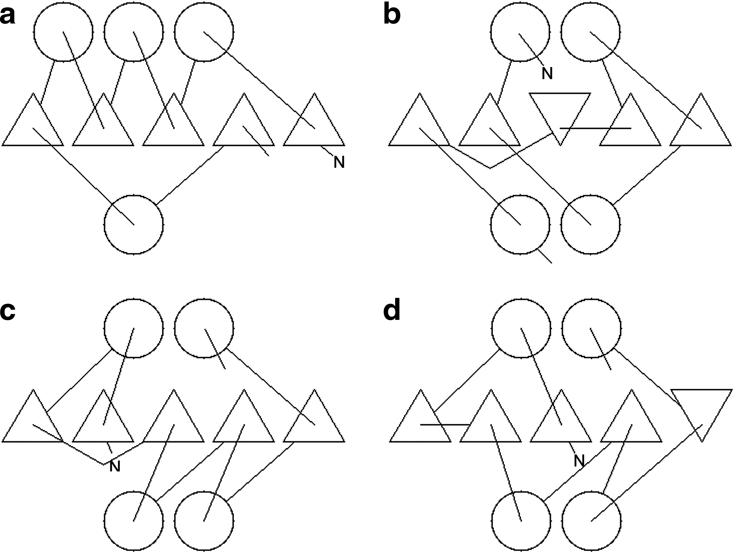
Most (top) and least (bottom) probable topologies from the “light” (left) and “dark” (right) sets.

4. Conclusion

In this work, we have shown that some of the accepted “rules” of protein topology that have been used over many years remain largely valid, while others lost discriminative power as increasing numbers of exceptions have been found. Those that remain are typically more complex, such as the “no-pretzel” rule, while the simpler rules (such as “no loop crossovers” or “no left-hand connections”) now have more violations.

Using these given rules, we fitted a general linear model to generate probabilities that could be used to assess known structures and others generated by structure prediction methods that included a large sample of folds not observed in the PDB. We found that most of these novel folds were equally likely under our model as those with known folds, indicating that their absence from the observed repertoire is not the result of any obvious bias in their construction.

Footnotes

Acknowledgments

The work was supported by the MRC National Institute for Medical Research, UK (U117581331). Inge Jonassen, James MacDonald and Jotun Hein are thanked for valuable discussion and comments.

Disclosure Statement

No competing financial interests exist.

1

They are not a true 2D representation as the information about whether the connections between SSEs pass over or under each other is retained.

2

To understand from a thermodynamic viewpoint why non-parallel structures are favorable we must look at the free energy of the structure and the fact that structures with low free energy are favorable [Finkelstein & Ptitsyn, 1987]. Using the “persistent chain model” [Flory, ] we see that the free energy of the connection is: \documentclass{aastex}\usepackage{amsbsy}\usepackage{amsfonts}\usepackage{amssymb}\usepackage{bm}\usepackage{mathrsfs}\usepackage{pifont}\usepackage{stmaryrd}\usepackage{textcomp}\usepackage{portland, xspace}\usepackage{amsmath, amsxtra}\pagestyle{empty}\DeclareMathSizes {10} {9} {7} {6}\begin{document}\begin{align*}\delta G = \frac{1}{2}RTa \int_{0}^{L} \left(\frac{d \vec{\theta}}{dx}\right)^{2} dx, \tag{1}\end{align*}\end{document}

where R is the gas constant, T is the absolute temperature, a is the persistent length, \documentclass{aastex}\usepackage{amsbsy}\usepackage{amsfonts}\usepackage{amssymb}\usepackage{bm}\usepackage{mathrsfs}\usepackage{pifont}\usepackage{stmaryrd}\usepackage{textcomp}\usepackage{portland, xspace}\usepackage{amsmath, amsxtra}\pagestyle{empty}\DeclareMathSizes {10} {9} {7} {6}\begin{document}\begin{align*}\frac{d \vec{\theta}}{dx}\end{align*}\end{document} is the curvature at the point x and L is the chain length. Assuming the curvature is approximately uniform it can be shown that the free energy for a parallel connection is approximately 4 times that of a non-parallel connection [Finkelstein & Ptitsyn, ]. This gives us considerable reason to favor non-parallel connections.

References

Cheng

, Grishin

N.V.

2005. DOM-fold: a structure with crossing loops found in DmpA, ornithine acetyltransferase, and molybdenum cofactor-binding protein domain. Prot. Sci., 14:1902–1910.

Cohen

F.E.

, Sternberg

M.J.E.

, Taylor

W.R.

1980. Analysis and prediction of protein β-sheet structures by a combinatorial approach. Nature, 285:378–382.

Cohen

F.E.

, Sternberg

M.J.E.

, Taylor

W.R.

1982. Analysis and prediction of the packing of α-helices against a β-sheet in the tertiary structure of globular proteins. J. Mol. Biol., 156:821–862.

Efimov

A.V.

1997. Structural trees for protein superfamilies. Proteins, 28:241–260.

Finkelstein

A.V.

, Ptitsyn

O.B.

1987. Why do globular proteins fit the limited set of folding patterns? Prog. Biophys. Mol. Biol., 50:171–190.

Flores

T.P.

, Moss

D.S.

, Thornton

J.M.

1994. An algorithm for automatically generating protein topology cartoons. Prot. Eng., 7:31–37.

Flory

P.J.

1969. Statistical Mechanics of Chain Molecules. Wiley-Interscience: New York.

Hinds

D.A.

, Levitt

1992. A lattice model for protein-structure prediction at low resolution. Proc. Natl. Acad. Sci. USA, 89:2536–2540.

Hou

, Sims

G.E.

, Zhang

et al. 2003. A global representation of protein fold space. Proc. Natl. Acad. Sci. USA, 100:2386–2390.

10.

Hutchinson

E.G.

, Thornton

J.M.

1993. The greek key motif-extraction, classification and analysis. Protein Engineering, 6:233–245.

11.

Luo

, Taylor

, Mezey

P.G.

1993. Vertex mobility of polyhedra. Bull. Math. Biol., 55:131–140.

12.

MacDonald

, Maksimiak

, Sadowski

et al. 2010. De novo backbone scaffolds for protein design. Proteins, 78:1311–1325.

13.

Nagano

1977. Logical analysis of the mechanism of protein folding: IV. super-secondary structures. J. Mol. Biol., 109:235–250.

14.

Orengo

C.A.

, Flores

T.P.

, Taylor

W.R.

et al. 1993. Identification and classification of protein fold families. Prot. Eng., 6:485–500.

15.

Richardson

1976. Handedness of crossover connections in beta-sheets. Proc. Natl. Acad. Sci. USA, 73:2619–2623.

16.

Richardson

J.S.

1977. β-Sheet topology and the relatedness of proteins. Nature, 268:495–500.

17.

Ruczinski

, Kooperberg

, Bonneau

et al. 2002. distributions of beta sheets in proteins with application to structure prediction. Proteins, 48:85–97.

18.

Sternberg

M.J.E.

, Thornton

J.M.

1977. On the conformation of proteins: the handedness of the connection between parallel β-strands. J. Mol. Biol., 110:269–283.

19.

Taylor

, Hollup

, MacDonald

et al. 2009. Probing the “dark matter” of protein fold-space. Structure, 17:1244–1252.

20.

Taylor

W.R.

2002. A periodic table for protein structure. Nature, 416:657–660.

21.

Taylor

W.R.

2007. Evolutionary transitions in protein fold space. Curr. Opin. Struct. Biol., 17:354–361.

22.

Taylor

W.R.

, Aszódi

2005. Protein Geometry, Classification, Topology and Symmetry. CRC Press: Boca Raton, FL.

23.

Taylor

W.R.

, Bartlett

G.J.

, Chelliah

et al. 2008. Prediction of protein structure from ideal forms. Proteins, 70:1610–1619.

24.

Woolfson

, Evans

, Hutchinson

et al. 1993. Topological and stereochemical restrictions in beta-sandwich protein structures. Prot. Eng., 6:461–470.

Supplementary Material

Please find the following supplemental material available below.

For Open Access articles published under a Creative Commons License, all supplemental material carries the same license as the article it is associated with.

For non-Open Access articles published, all supplemental material carries a non-exclusive license, and permission requests for re-use of supplemental material or any part of supplemental material shall be sent directly to the copyright owner as specified in the copyright notice associated with the article.

0.00 MB

0.09 MB