On the A-Optimality Criterion for Finding Two-Color Microarray Optimal Designs

Abstract

Several studies on two-color microarray experimental designs consider the A-optimality criterion for the assessment and/or search of appropriate/optimal designs. What seems to be widely ignored, however, is the well-known fact that A-optimal designs depend on the choice of scale or code combination of the X-variables. In this article, it is shown that intrinsically different optimal microarray designs will be obtained depending on the chosen code combination of the qualitative factors. Moreover, a substantial loss in efficiency will result when a design, which is optimal for a specific code combination, is used for another one. This coding problematic is also applicable to the admissibility concept.

1. Introduction

Articles on experimental designs for two-color microarray are many. Since the pioneering studies of Kerr and Churchill (2001) and Yang and Speed (2002), a variety of others appeared, differing in their underlying statistical models and/or searching techniques (Kerr et al., 2000; Rosa et al., 2005; Landgrebe et al., 2006). In all of them, the use of certain criteria was needed in order to assess designs' statistical efficiency and/or search of optimal ones. Such statistical criteria are well known in the experimental design literature and usually referred to as the alphabetical optimality criteria (Atkinson and Donev, 1992). Among them, the A-optimality criterion has been repeatedly applied in microarray (Kerr and Churchill, 2001; Yang and Speed, 2002; Bailey, 2007).

The A-criterion's wide appeal lies in its straightforward interpretation and numerically simple computation. For A-optimal designs, the regression parameter estimates of the underlying regression model have a minimum average variance. However, what seems to be broadly neglected is the fact that A-optimal designs depend on the choice of scale or code combination of the explanatory X-variables. As reflected by its frequent use in microarray design studies, the A-optimal design scale dependence seems to be taken too lightly, as if it were a minor feature, easily negligible. Such conduct, however, is not characteristic for the microarray community alone. It is generally overlooked in experimental settings, in which explanatory variables are qualitative. As Atkinson and Donev (1992, pg 107) claim: “For designs with all factors qualitative … the problem of scale does not arise” (see also Bailey, 2007).

Herein, this (mis)conception will be briefly revisited. By means of a 2 × 2 time-course microarray experiment (Glonek and Solomon, 2004), it will be shown that different A-optimal designs will be found depending on the chosen code combination of the qualitative factors (Section 2). Moreover, inter-designs comparisons reveal that code-switching may also result in substantial loss of efficiency (Section 3). Finally, on the grounds of the code-dependence of the A-optimality criterion, of the arbitrariness of coding, and of possible efficiency loss, which may have substantial impact on the experimental costs, the utility of this criterion in the microrarray context is re-evaluated.

2. Methods

Consider a study in which two experimental conditions are to be compared. Suppose for simplicity that for each condition there is only one gene, whose expression will be measured on different subjects at time points a and b (a < b), respectively. The outcome is the intensity of expressed cDNA measured at two different time points. A possible method to explain the variation in intensity of expressed cDNA is by means of a regression model: \documentclass{aastex}\usepackage{amsbsy}\usepackage{amsfonts}\usepackage{amssymb}\usepackage{bm}\usepackage{mathrsfs}\usepackage{pifont}\usepackage{stmaryrd}\usepackage{textcomp}\usepackage{portland,xspace}\usepackage{amsmath,amsxtra}\pagestyle{empty}\DeclareMathSizes{10}{9}{7}{6} \begin{document} \begin{align*} \ln ( I ) = \beta_0 + \beta_1 Time + \beta_2 Cond + \beta_3 Int + \varepsilon , \tag{1} \end{align*} \end{document}

where I is the intensity of the expressed cDNA, the variable Time is dichotomous at time points a and b, a < b, the variable Cond is dichotomous with codes c and d, respectively, and the term Int is the interaction between Time and Cond. The regression parameters are denoted by β_i, i = 0, … , 3, and ɛ is the usual disturbance term.

In this setting, there are four possible time/condition combinations, resulting in four biological groups. For example, a comparison can be made between the gene expression of the experimental condition c at time point a, and that of the same experimental condition at time point b. This differential gene expression can be interpreted as the change in expression from time point a to time point b. For simplicity, dye- bias will be assumed to be non-existent. This comparison can be visualized by means of an undirected graph (neglecting the dye effect). This can be represented by a set of vertices or “nodes” and a collection of edges that connect pairs of vertices. Figure 1 shows an example of one comparison (cohybridization) that henceforth is referred to as “configuration” (Glonek and Solomon, 2004).

FIG. 1.

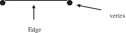
Example of an undirected graph.

With four different groups (time × conditions), there are in total six ways of pair-wise combining them in a microarray slide. Figure 2 shows all possible configurations represented as a graph with four vertices (groups) and six edges (configurations).

FIG. 2.

Schematic visualization of the possible configurations.

Configuration 2 in the graph, for example, represents the differential gene-expression between the two experimental conditions at time point a and can be expressed in terms of the regression parameters of model (1). The expected differential gene-expression E(Δ(ln (I))) for configuration 2 is equal to \documentclass{aastex}\usepackage{amsbsy}\usepackage{amsfonts}\usepackage{amssymb}\usepackage{bm}\usepackage{mathrsfs}\usepackage{pifont}\usepackage{stmaryrd}\usepackage{textcomp}\usepackage{portland,xspace}\usepackage{amsmath,amsxtra}\pagestyle{empty}\DeclareMathSizes{10}{9}{7}{6} \begin{document} $$ ( \beta_0 + \beta_1 a + \beta_2 d + \beta_3 ad ) - ( \beta_0 + \beta_1 a + \beta_2 c + \beta_3 ac ) = \beta_2 ( d - c ) + \beta_3 a ( d - c ) $$ \end{document} , which is a function of the regression parameters (Table 1).

Table 1.

A 2 × 2 Time-Course Design

Intensity of		Time
Expressed cDNA		a	b
	c	\documentclass{aastex}\usepackage{amsbsy}\usepackage{amsfonts}\usepackage{amssymb}\usepackage{bm}\usepackage{mathrsfs}\usepackage{pifont}\usepackage{stmaryrd}\usepackage{textcomp}\usepackage{portland,xspace}\usepackage{amsmath,amsxtra}\pagestyle{empty}\DeclareMathSizes{10}{9}{7}{6} \begin{document} $$ \beta_0 + \beta_1 a + \beta_2 c + \beta_3 ac$$ \end{document}	\documentclass{aastex}\usepackage{amsbsy}\usepackage{amsfonts}\usepackage{amssymb}\usepackage{bm}\usepackage{mathrsfs}\usepackage{pifont}\usepackage{stmaryrd}\usepackage{textcomp}\usepackage{portland,xspace}\usepackage{amsmath,amsxtra}\pagestyle{empty}\DeclareMathSizes{10}{9}{7}{6} \begin{document} $$ \beta_0 + \beta_1 b + \beta_2 c + \beta_3 bc$$ \end{document}
Exp.cond.
	d	\documentclass{aastex}\usepackage{amsbsy}\usepackage{amsfonts}\usepackage{amssymb}\usepackage{bm}\usepackage{mathrsfs}\usepackage{pifont}\usepackage{stmaryrd}\usepackage{textcomp}\usepackage{portland,xspace}\usepackage{amsmath,amsxtra}\pagestyle{empty}\DeclareMathSizes{10}{9}{7}{6} \begin{document} $$ \beta_0 + \beta_1 a + \beta_2 d + \beta_3 ad$$ \end{document}	\documentclass{aastex}\usepackage{amsbsy}\usepackage{amsfonts}\usepackage{amssymb}\usepackage{bm}\usepackage{mathrsfs}\usepackage{pifont}\usepackage{stmaryrd}\usepackage{textcomp}\usepackage{portland,xspace}\usepackage{amsmath,amsxtra}\pagestyle{empty}\DeclareMathSizes{10}{9}{7}{6} \begin{document} $$ \beta_0 + \beta_1 b + \beta_2 d + \beta_3 bd$$ \end{document}

Usually, the codes of the condition variable and the time points are known and chosen by the researcher. Table 2 shows the other configurations as a function of the regression parameters.

Table 2.

All Configurations as a Function of the Regression Parameters

Configuration	Expected Δ(ln (I))
1	\documentclass{aastex}\usepackage{amsbsy}\usepackage{amsfonts}\usepackage{amssymb}\usepackage{bm}\usepackage{mathrsfs}\usepackage{pifont}\usepackage{stmaryrd}\usepackage{textcomp}\usepackage{portland,xspace}\usepackage{amsmath,amsxtra}\pagestyle{empty}\DeclareMathSizes{10}{9}{7}{6} \begin{document} $$ \beta_1 ( b - a ) + \beta_3 c ( b - a )$$ \end{document}
2	\documentclass{aastex}\usepackage{amsbsy}\usepackage{amsfonts}\usepackage{amssymb}\usepackage{bm}\usepackage{mathrsfs}\usepackage{pifont}\usepackage{stmaryrd}\usepackage{textcomp}\usepackage{portland,xspace}\usepackage{amsmath,amsxtra}\pagestyle{empty}\DeclareMathSizes{10}{9}{7}{6} \begin{document} $$ \beta_2 ( d - c ) + \beta_3 a ( d - c )$$ \end{document}
3	\documentclass{aastex}\usepackage{amsbsy}\usepackage{amsfonts}\usepackage{amssymb}\usepackage{bm}\usepackage{mathrsfs}\usepackage{pifont}\usepackage{stmaryrd}\usepackage{textcomp}\usepackage{portland,xspace}\usepackage{amsmath,amsxtra}\pagestyle{empty}\DeclareMathSizes{10}{9}{7}{6} \begin{document} $$ \beta_1 ( b - a ) + \beta_2 ( d - c ) + \beta_3 ( bd - ac )$$ \end{document}
4	\documentclass{aastex}\usepackage{amsbsy}\usepackage{amsfonts}\usepackage{amssymb}\usepackage{bm}\usepackage{mathrsfs}\usepackage{pifont}\usepackage{stmaryrd}\usepackage{textcomp}\usepackage{portland,xspace}\usepackage{amsmath,amsxtra}\pagestyle{empty}\DeclareMathSizes{10}{9}{7}{6} \begin{document} $$ \beta_2 ( d - c ) + \beta_3 b ( d - c )$$ \end{document}
5	\documentclass{aastex}\usepackage{amsbsy}\usepackage{amsfonts}\usepackage{amssymb}\usepackage{bm}\usepackage{mathrsfs}\usepackage{pifont}\usepackage{stmaryrd}\usepackage{textcomp}\usepackage{portland,xspace}\usepackage{amsmath,amsxtra}\pagestyle{empty}\DeclareMathSizes{10}{9}{7}{6} \begin{document} $$ \beta_1 ( b - a ) + \beta_3 d ( b - a )$$ \end{document}
6	\documentclass{aastex}\usepackage{amsbsy}\usepackage{amsfonts}\usepackage{amssymb}\usepackage{bm}\usepackage{mathrsfs}\usepackage{pifont}\usepackage{stmaryrd}\usepackage{textcomp}\usepackage{portland,xspace}\usepackage{amsmath,amsxtra}\pagestyle{empty}\DeclareMathSizes{10}{9}{7}{6} \begin{document} $$ \beta_1 ( b - a ) + \beta_2 ( c - d ) + \beta_3 ( bc - ad )$$ \end{document}

The problem of optimal design concerns allocating microarray slides to those configurations, for which the regression parameters (β₁, β₂, and β₃) can be estimated as precise as possible. This can be accomplished using methods that are customary in the optimal design literature (Kerr, 2001; Rosa, 2006). Note from Table 2 that the differential gene expression Y = Δ(ln (I)) can be written as a linear fixed-effects regression model as follows: \documentclass{aastex}\usepackage{amsbsy}\usepackage{amsfonts}\usepackage{amssymb}\usepackage{bm}\usepackage{mathrsfs}\usepackage{pifont}\usepackage{stmaryrd}\usepackage{textcomp}\usepackage{portland,xspace}\usepackage{amsmath,amsxtra}\pagestyle{empty}\DeclareMathSizes{10}{9}{7}{6} \begin{document} \begin{align*} { Y} = { X} \beta + \varepsilon , \tag{2} \end{align*} \end{document}

with outcome Y as an S × 1 vector with component Y_s, s = 1, … , S representing the differential gene expression of s-th microarray, an S × p design matrix X, for which each row consists of a representative of one of the S configurations, the number of columns p is the length of the vector of regression parameters β = (β₁, … , β_p)′ and ɛ is the S × 1 vector of disturbances assumed to be normally distributed with mean zero and variance σ²_ɛ I_{S x S}. The matrix I_{S x S} is the S × S identity matrix.

The maximum likelihood method leads to the asymptotic variance-covariance matrix: \documentclass{aastex}\usepackage{amsbsy}\usepackage{amsfonts}\usepackage{amssymb}\usepackage{bm}\usepackage{mathrsfs}\usepackage{pifont}\usepackage{stmaryrd}\usepackage{textcomp}\usepackage{portland,xspace}\usepackage{amsmath,amsxtra}\pagestyle{empty}\DeclareMathSizes{10}{9}{7}{6} \begin{document} \begin{align*} { \rm var}{ \left( { \hat \beta} \right) } \approx \left( X^t WX \right) ^{ - 1} , \tag{3} \end{align*} \end{document}

with the S × S diagonal matrix of weights W. Each diagonal element w_i, i = 1, … , S represents the fraction of configuration i. The interest lies in the optimization of the variance-covariance matrix \documentclass{aastex}\usepackage{amsbsy}\usepackage{amsfonts}\usepackage{amssymb}\usepackage{bm}\usepackage{mathrsfs}\usepackage{pifont}\usepackage{stmaryrd}\usepackage{textcomp}\usepackage{portland,xspace}\usepackage{amsmath,amsxtra}\pagestyle{empty}\DeclareMathSizes{10}{9}{7}{6} \begin{document} $${ \rm var}{ \left( { \hat \beta} \right)}$$ \end{document} . If \documentclass{aastex}\usepackage{amsbsy}\usepackage{amsfonts}\usepackage{amssymb}\usepackage{bm}\usepackage{mathrsfs}\usepackage{pifont}\usepackage{stmaryrd}\usepackage{textcomp}\usepackage{portland,xspace}\usepackage{amsmath,amsxtra}\pagestyle{empty}\DeclareMathSizes{10}{9}{7}{6} \begin{document} $${ \hat \beta}$$ \end{document} is a scalar, then the variance-covariance also reduces to a scalar. The optimal design is in this situation the design for which \documentclass{aastex}\usepackage{amsbsy}\usepackage{amsfonts}\usepackage{amssymb}\usepackage{bm}\usepackage{mathrsfs}\usepackage{pifont}\usepackage{stmaryrd}\usepackage{textcomp}\usepackage{portland,xspace}\usepackage{amsmath,amsxtra}\pagestyle{empty}\DeclareMathSizes{10}{9}{7}{6} \begin{document} $${\rm var}{ \left( { \hat \beta} \right) }$$ \end{document} is smallest. If \documentclass{aastex}\usepackage{amsbsy}\usepackage{amsfonts}\usepackage{amssymb}\usepackage{bm}\usepackage{mathrsfs}\usepackage{pifont}\usepackage{stmaryrd}\usepackage{textcomp}\usepackage{portland,xspace}\usepackage{amsmath,amsxtra}\pagestyle{empty}\DeclareMathSizes{10}{9}{7}{6} \begin{document} $${ \hat \beta}$$ \end{document} is a matrix, then \documentclass{aastex}\usepackage{amsbsy}\usepackage{amsfonts}\usepackage{amssymb}\usepackage{bm}\usepackage{mathrsfs}\usepackage{pifont}\usepackage{stmaryrd}\usepackage{textcomp}\usepackage{portland,xspace}\usepackage{amsmath,amsxtra}\pagestyle{empty}\DeclareMathSizes{10}{9}{7}{6} \begin{document} $${ \rm var}{ \left( { \hat \beta} \right) }$$ \end{document} cannot be ordered without the use of a mapping onto a one-dimensional space. A commonly used mapping is to take the average of the variances of the regression parameter estimates. The optimal design is the design for which the average variance is smallest. The criterion based on this mapping, is called the A-optimality criterion (Atkinson and Donev, 1992). In the next section, some results are presented to illustrate the effect of code combination of the independent variables on the A-optimal design of a microarray experiment.

3. Results

In the 2 × 2 time course example, there are six different configurations and three regression parameters, i.e., S = 6 and p = 3, respectively. The design matrix X is equal to \documentclass{aastex}\usepackage{amsbsy}\usepackage{amsfonts}\usepackage{amssymb}\usepackage{bm}\usepackage{mathrsfs}\usepackage{pifont}\usepackage{stmaryrd}\usepackage{textcomp}\usepackage{portland,xspace}\usepackage{amsmath,amsxtra}\pagestyle{empty}\DeclareMathSizes{10}{9}{7}{6} \begin{document} \begin{align*} X = \left( \begin{matrix}b - a & 0 & c ( b - a ) \\ 0 & d - c & a ( d - c ) \\ b - a & d - c & bd - ac \\ 0 & d - c & b ( d - c ) \\ b - a & 0 & d ( b - a ) \\ b - a & c - d & bc - ad\end{matrix} \right). \tag{4} \end{align*} \end{document}

Using the nonlinear minimization algorithm developed by Nelder and Mead (see MATLAB version 7.0.1 [R14]) (Molenberghs et al., 2006), the A-optimal weights of the design points (configurations) can be determined for different code combinations of the X-variables. Table 3 shows some results. For ease of presentation, it is supposed that the first time point a is equal to the smallest code c of the treatment variable (a = c) and the second time point b is equal to the largest code d of the treatment variable (b = d). From Table 3, it can be seen that the A-optimal for the code combination −1/1 is a uniform design, i.e., all 6 configurations were selected and assigned equal weight. The upper part of Figure 3 shows the optimal combination of configurations when the total number of arrays is restricted to six. If, however, the code combination 0/1 is used, then for the A-optimal design twice as many slides would be allocated to configurations 1 and 2 than to 4 and 5, and none whatsoever to 3 and 6. The bottom design of Figure 3 shows the corresponding undirected graph of the 0/1 A-optimal design. It is apparent that different optimal designs are obtained depending on the used coding. Note that, for code combination 0/2, the exact A–optimal design coincides with the one from the 0/1 coding when the number of slides is equal to 6. This concordance, however, will disappear once the number of available slides increases (e.g., larger than 24).

FIG. 3.

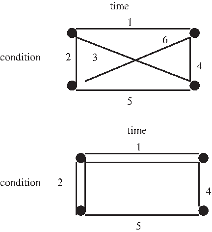
Optimal two-color microarray designs for two different code combinations.

Table 3.

A-Optimal Approximate Weights for Different Code Combination, Using the Nelder-Mead Simplex Method

{c, d} a = c, b = d	w ₁	w ₂	w ₃	w ₄	w ₅	w ₆
{−1, 1}	0.17	0.17	0.17	0.17	0.16	0.16
{0, 1}	0.32	0.32	0	0.18	0.18	0
{0, 2}	0.36	0.36	0	0.12	0.12	0.04
{0, 10}	0.40	0.40	0.02	0.02	0.02	0.14

Glonek and Solomon (2004) used a different criterion for assessment of two-color microarray designs based on admissibility concept. Admissible designs are those, for which there exists no other design providing at least as accurate estimates of all parameters and for at least one strict more accurate estimate (Glonek and Solomon, 2004). Recall that an A-optimal design minimizes the average variance of all parameter estimates. Given the admissibility definition, an A-optimal design is always an admissible design, but the opposite does not necessarily apply.

It is noteworthy that the bottom design of Figure 3 was identified by Glonek and Solomon (2004) as an admissible design for a given number of 6 arrays. The uniform design (A-optimal for the coding −1/1), on the other hand, was never mentioned. This is understandable, since the uniform design is neither admissible nor A-optimal under the coding 0/1 (the implicit codes used in the examples of Glonek and Solomon). Had the authors considered a different coding (-1/1), the admissibility of the uniform design would have emerged. Thus, this shows that scale-dependence also affects designs based on the admissibility criterion.

Designs' comparisons

Suppose that a design is A-optimal for some arbitrary code combination. What would happen to this design's A-efficiency if another coding were used? Note that the whole idea of the code's effect on A-optimal designs would be immaterial, were the optimal designs, obtained for different codes, to remain highly efficient with respect to each other. To check this possibility, inter-designs comparisons are necessary and a common gauge for these performance comparisons are the designs' relative efficiencies. The A-relative efficiency of a design with coding {c, d} with respect to coding {c₁, d₁} is defined as: \documentclass{aastex}\usepackage{amsbsy}\usepackage{amsfonts}\usepackage{amssymb}\usepackage{bm}\usepackage{mathrsfs}\usepackage{pifont}\usepackage{stmaryrd}\usepackage{textcomp}\usepackage{portland,xspace}\usepackage{amsmath,amsxtra}\pagestyle{empty}\DeclareMathSizes{10}{9}{7}{6} \begin{document} \begin{align*} { \rm rel } . { \rm eff } \left( \xi_ { \{ c , d \} } \mid \xi_ { \{ c_1 , d_1 \} } \right) = \frac { { \rm Tr } \left( { \rm var } \left( { \hat \beta } _ { \{ c_1 , d_1 \} } \right) \right) } { { \rm Tr } \left( { \rm var } \left( { \hat \beta } _ { \{ c , d \} } \right) \right) } , \tag { 5 } \end{align*} \end{document}

With ξ_{c,d} and \documentclass{aastex}\usepackage{amsbsy}\usepackage{amsfonts}\usepackage{amssymb}\usepackage{bm}\usepackage{mathrsfs}\usepackage{pifont}\usepackage{stmaryrd}\usepackage{textcomp}\usepackage{portland,xspace}\usepackage{amsmath,amsxtra}\pagestyle{empty}\DeclareMathSizes{10}{9}{7}{6} \begin{document} $$ \xi_{ \{ c_1 , d_1 \} }$$ \end{document} as the A-optimal design when {c, d} or {c₁, d₁} is used as the code combination, respectively. \documentclass{aastex}\usepackage{amsbsy}\usepackage{amsfonts}\usepackage{amssymb}\usepackage{bm}\usepackage{mathrsfs}\usepackage{pifont}\usepackage{stmaryrd}\usepackage{textcomp}\usepackage{portland,xspace}\usepackage{amsmath,amsxtra}\pagestyle{empty}\DeclareMathSizes{10}{9}{7}{6} \begin{document} $${ \rm Tr} \left( { \rm var} \left( { \hat \beta}_{ \{ c , d \} } \right) \right) $$ \end{document} is the trace of the variance-covariance of the regression parameter estimates when using the {c, d} code combination.

Table 4 displays the approximate (for large numbers of slides) relative efficiencies of A-optimal designs found for the following codes: 0/1, −1/1, 0/2, and 0/10, after a code-change took place. For instance, the uniform design, which is A-optimal for −1/1, has a relative efficiency equal to 0.79 when the code combination 0/1 is instead applied. In practical terms this means that about 20% more arrays will have to be added to the original −1/1 A-optimal design, if the researchers decided to use instead the 0/1 coding. Considering the relative arbitrariness of coding, this result strikes at first as pointless, if not absurd. Unfortunately, a careful appreciation does not change the unfavorable picture. Moreover, note also that the highest efficiency loss affects the 0/10 A-optimal design (60–70% in Table 4). Given its apparent unconventionality, one may think of this example (0/10) as a slight exaggeration, specifically chosen to emphatically make a point of the pitfalls of A-optimal designs. However, this coding may not represent that great a departure from reality. In a time course microarray experiment, for instance, in which time (measured in minutes, for example) is categorized (0, 10, 20 …), researchers often take over the original coding of the dataset, representing the minutes, both for the analysis and/or for the preceding design stage, unaware of the effects that this may have on the search of an optimal designs. The relative efficiencies presented in Table 4 are computed based on the A–optimal designs, whose approximate weight distribution are found in Table 3. A similar pattern of efficiency loss will be found for the exact designs.

Table 4.

A-Relative Efficiency of an Approximate Design that Is Optimal in {c₁, d₁} if {c, d} Is Used Instead (a = c, b = d)

	Design that is optimal in
Used in code combination		{−1, 1}	{0, 1}	{0, 2}	{0, 10}
	{−1, 1}	1	0.86	0.76	0.31
	{0, 1}	0.79	1	0.93	0.42
	{0, 2}	0.79	0.96	1	0.70
	{0, 10}	0.67	0.79	0.89	1

4. Conclusion

In the last decade, rather advanced statistical tools have been applied to obtain the best possible microarray designs in terms of practical convenience, costs, and statistical efficiency. Irrespective of the different experimental settings, underlying gene expression models, and optimal design searching techniques, they all have their foundation on the theory of existing statistical methods of design optimisation.

For designs' efficiency assessment, a statistical criterion is required in order to identify the most appropriate ones. The A-optimality criterion is often mentioned in the literature and widely applied in practice. In the present article, we attempted to show that the indiscriminative use of the A-optimality criterion has a serious drawback whose unawareness or dismissal may have undesirable consequences.

For the sake of argument, let's assume that researchers seek expert advice in bibliographic references as how to set up their experiments. They want to find the best arrangement of co-hybridizations among the several biological groups to be compared. Unacquainted with the scale-dependence of A-optimal designs, they may easily apply a design described in a publication as optimal for their experimental conditions, whose coding was omitted (as is usually the case). Their own coding system, however, happens to differ from the ones in the optimal design article. What follows is that the applied design will no longer be the most efficient one for estimating the effects of interest. As a result, their model parameter estimates may be inefficient, their statistical tests possibly underpowered and differential gene expression may no longer be detectable. The easier solution of increasing the number biological replications (new subjects and arrays), given the prohibitive costs of microarray, is not usually the most viable one.

The best way out of this impasse would be using those optimality criteria, whose designs have been proven to be scale invariant. The D-optimality criterion, for instance, is one of them. It minimizes the joint confidence ellipsoid of all, or a linear combination of the regression parameter estimates, which is reached by minimizing the determinant of \documentclass{aastex}\usepackage{amsbsy}\usepackage{amsfonts}\usepackage{amssymb}\usepackage{bm}\usepackage{mathrsfs}\usepackage{pifont}\usepackage{stmaryrd}\usepackage{textcomp}\usepackage{portland,xspace}\usepackage{amsmath,amsxtra}\pagestyle{empty}\DeclareMathSizes{10}{9}{7}{6} \begin{document} $${ \rm var} \left( { \hat \beta} \right) $$ \end{document} . It has also being applied to microarray experiments (Bailey, 2007).

Given the A-optimality criterion's wide application, easy interpretation, and simple numerical computation, it is unlikely that its current status as one of the favorite criteria will be changed in foreseeable future. Hence, this note of caution is meant to remind practitioners and optimal designs experts to choose their coding consistent with the research questions of interest and to always report the underlying coding system when dealing with design issues. That said, even if these recommendations are accommodated, they will have more a palliative than a remedial effect. There is no such a thing as a convenient coding that is completely devoid of some degree of arbitrariness.

Footnotes

Disclosure Statement

No competing financial interests exist.

References

Atkinson

G.L.

, Donev

A.N.

1992. Optimum Experimental Designs. Clarendon Press: Oxford, UK.

Bailey

R.A.

2007. Designs for two-color microarray experiments. Appl. Stat., 56:365–394.

Glonek

G.F.V.

, Solomon

P.J

. 2004. Factorial and time course designs cDNA microarray experiments. Biostatistics, 5:89–111.

Kerr

M.K.

, Martin

, Churchill

G.A.

2000. Analysis of variance for gene expression microarray data. J. Comput. Biol., 7:819–837.

Kerr

M.K.

, Churchill

G.A.

2001. Experimental design for gene expression microarrays. Biostatistics, 2:183–201.

Landgrebe

, Bretz

, Brunner

2006. Efficient design and analysis of two color factorial microarray experiments. Comput. Stat. Data Anal., 50:499–517.

Molenberghs

, Tuerlinckx

, Verbeke

2006. Numerical Techniques for Statisticians. University Hasselt and Catholic University: Leuven.

Rosa

G.J.M.

, Steibel

J.P.

, Tempelman

R.J.

2005. Reassessing design and analysis of two color microarray experiments using mixed effects models. Comp. Funct. Genomics, 6:123–131.

Yang

Y.H.

, Speed

2002. Design issues for cDNA microarray experiments. Nat. Rev., 3:579–588.