A Polynomial-Time Algorithm Computing Lower and Upper Bounds of the Rooted Subtree Prune and Regraft Distance

Abstract

Rooted, leaf-labeled trees are used in biology to represent hierarchical relationships of various entities, most notably the evolutionary history of molecules and organisms. Rooted Subtree Prune and Regraft (rSPR) operation is a tree rearrangement operation that is used to transform a tree into another tree that has the same set of leaf labels. The minimum number of rSPR operations that transform one tree into another is denoted by d_rSPR and gives a measure of dissimilarity between the trees, which can be used to compare trees obtained by different approaches, or, in the context of phylogenetic analysis, to detect horizontal gene transfer events by finding incongruences between trees of different evolving characters. The problem of computing the exact d_rSPR measure is NP-hard, and most algorithms resort to finding sequences of rSPR operations that are sufficient for transforming one tree into another, thereby giving upper bound heuristics for the distance. In this article, we present an O(n⁴) recursive algorithm D-Clust that gives both lower bound and upper bound heuristics for the distance between trees with n shared leaves and also gives a sequence of operations that transforms one tree into another. Our experiments on simulated pairs of trees containing up to 100 leaves showed that the two bounds are almost equal for small distances, thereby giving the nearly-precise actual value, and that the upper bound tends to be close to the upper bounds given by other approaches for all pairs of trees.

1. Introduction

Rooted, leaf-labeled trees (“trees” for short in this article) are a type of directed acyclic graphs that are widely used in biology. Phylogenetic analysis of genes, species, or other operational taxonomic units (OTUs) is one familiar application that seeks to reconstruct the evolutionary history of the OTUs in the form of a tree. In a non-phylogenetic setting, the genome-wide series of measurements, for example, gene expression readouts, may be hierarchically clustered by similarity of expression patterns, with the resulting solution also represented as a tree. More generally, it has been shown that many types of networks of different topologies observed in real-life complex systems, including living cells, can be transformed into hierarchical clusters without loss of certain essential properties, such as the modular structure (Clauset et al., 2008). Thus, trees are useful for analysis of many biological phenomena. In this article, we deal with an important subclass of trees, namely rooted binary trees with unweighted edges. The goal of our study is to estimate the sequence of operations that transforms one tree to another, when the two trees have the same set of labels on the terminal branches (leaves).

The subtree prune and regraft (SPR) distance is a well-known tree distance measure that has been applied for comparison of biological trees, especially for finding differences between phylogenetic trees, for example, when the accuracy of tree inference method is compared to a standard solution or when phylogenies of different characters are compared to find the amount of disagreement between topologies; this disagreement can be the evidence of bias of the data or of unusual evolutionary events, such as hybridization or horizontal gene transfer (Hein, 1990; Wang et al., 2001; Song and Hein, 2005; Baroni et al., 2005). When applied to rooted trees, the distance takes the form of a rooted Subtree Prune and Regraft (rSPR) operation, which is a rearrangement that detaches a subtree from the tree and attaches it on another branch of the tree (see below for the formal definition). The rooted SPR measure, d_rSPR between two trees which have the same set of leaf labels is the minimum number of rSPR operations that transform one tree into another. In the case of phylogenetic trees, the sequence of transforming operations can be used to identify the lineages involved in horizontal gene transfer (Than et al., 2008).

The problem of computing the d_rSPR distance was shown in Bordewich and Semple (2004) to be a NP-hard. They also proved that the problem is fixed parameter tractable with respect to the unknown distance k, (i.e.) there is an algorithm whose computational complexity is (56 k) p(n), where p(n) is a polynomial in n, the number of leaves shared between the trees. Heuristic algorithms to compute the d_rSPR distance between trees include upper bound finding algorithms, namely LatTrans (Hallett and Lagergren, 2001), HorizStory (MacLeod et al., 2005), EEEP (Beiko and Hamilton, 2006), TNT (Goloboff, 2007), and the RIATA-HGT (Nakhleh et al., 2005) algorithm in the Phylonet software (Than et al., 2008). All of them provide sequences of rSPR operations that transform one tree into another, and thereby give upper bounds for the measure. Another class of algorithms, such as SPRDist (Wu, 2009) and SPRIT (Hill et al., 2010) give the exact distance between the trees. SPRDist employs an integer programming approach that uses the connection between the maximum agreement forest (MAF) (Hein et al., 1996) and the d_rSPR distance. Although finding the d_rSPR distance using this approach is also NP-hard, it has been shown that SPRDist runs efficiently for trees with 40 or fewer leaves and for tree pairs with small d_rSPR values. However, the algorithm does not provide the set of rSPR operations for the transformation. The most recent algorithm SPRIT uses an exhaustive method and utilizes a conjecture to reduce the search space, to provide the exact distance and the minimum number of transforming operations.

In this work, we provide a new algorithm D-Clust that gives both an upper bound and a lower bound for the d_rSPR distance for a pair of trees that share leaf labels, as well as the sequence of operations that transforms one tree into another and whose number of operations is equal to the upper bound. We examined the accuracy of D-Clust on the simulated trees with known d_rSPR and found that its upper bound is very close to that given by the other algorithms. Moreover, for the small values of d_rSPR and large values of n, i.e., the situation mimicking the low level of horizontal gene transfer between genomes, the lower bound is efficiently computed by D-Clust and tends to be the same as the upper bound, thus providing the actual distance.

2. Methods

2.1. Definitions

We denote the set of all binary trees with a given set X as B(X). Throughout the paper, let the cardinality of X be denoted as n. For the upcoming discussions, let \documentclass{aastex}\usepackage{amsbsy}\usepackage{amsfonts}\usepackage{amssymb}\usepackage{bm}\usepackage{mathrsfs}\usepackage{pifont}\usepackage{stmaryrd}\usepackage{textcomp}\usepackage{portland,xspace}\usepackage{amsmath,amsxtra}\pagestyle{empty}\DeclareMathSizes{10}{9}{7}{6}\begin{document}$$T, T_1, T_2 \in B (X)$$\end{document} . We employ some graph theoretical terminology used in Diestel (2005) in our definitions. The edges of the trees in B(X) are assumed to be directed away from the root (not shown in the figures); this is not strictly necessary for the definitions, but aids the explanation. In this article, we restrict our explanations to binary trees, although most of the results can be extended to multifurcating trees as well.

Descendant and ancestor of a vertex in T

Let u, v be two vertices in T. We say that v is a descendant of u if the path from the root to v contains u, and an ancestor of u if the path from the root to u contains v.

Subtrees of a tree rooted at a vertex

We call the induced subgraph of T that contains the vertex v of T and all its descendants, as the subtree of T rooted at v and denote it by S_v (Fig. 1).

FIG. 1.

In the tree T, C : = {a, b, c} is the set of all label descendants of the vertex 1, and hence it is a cluster in T. The subgraph S₁ of T inside the triangle is the subtree of T rooted at the vertex 1. Also note that S₁ = T|C.

Clusters in a tree

A cluster C in T is the subset of X such that C is a set of all label descendants of a vertex in T (Fig. 1). We call the cluster X and all the singleton clusters as trivial clusters in T, and the remaining clusters as non-trivial. We denote the set of all non-trivial clusters in T as C(T). Note that the tree topology of T can be revealed by listing all the clusters in T.

Subtree of a tree induced by a leaf set

Suppose Y is a subset of X. Let \documentclass{aastex}\usepackage{amsbsy}\usepackage{amsfonts}\usepackage{amssymb}\usepackage{bm}\usepackage{mathrsfs}\usepackage{pifont}\usepackage{stmaryrd}\usepackage{textcomp}\usepackage{portland,xspace}\usepackage{amsmath,amsxtra}\pagestyle{empty}\DeclareMathSizes{10}{9}{7}{6}\begin{document}$$Z = Y \cup \{z: z \ \hbox{\rm is an ancestor of a vertex} \ y \in Y \}$$\end{document} . The subgraph of T induced by Z is a rooted tree with Y as the set of its leaf labels. We call this tree as the subtree of T induced by Y and denote it by T|Y (Fig. 1).

SPR operation on a tree

Let e = (u, v) be an edge in T such that v is a descendant of u. A rooted SPR operation (rSPR) on the binary tree T is performed by first removing the edge e that results in a graph with two components, one of which is S_v (the subtree rooted at v), and T − S_v; and then performing one of the two steps:

(i) replace an edge e = (a, b) in T − S_v by the edges (a, u′) and (u′, b), where u′ is a new vertex, and add the edge (u′, v), thus connecting S_v and T − S_v, or

(ii) add a dummy leaf with label “r” incident at the root of T − S_v, add an edge between r and v and let r be the root of the new tree.

The resulting tree is also a rooted binary tree with n leaves and the subtree S_v is called the rSPR subtree. We also refer to a rSPR subtree by the subtree T|C, where C is the set of all leaves of S_v. See Figure 2 for an illustration of two rSPR operations—the first using the step (ii) and the second using the step (i)—performed on a tree.

FIG. 2.

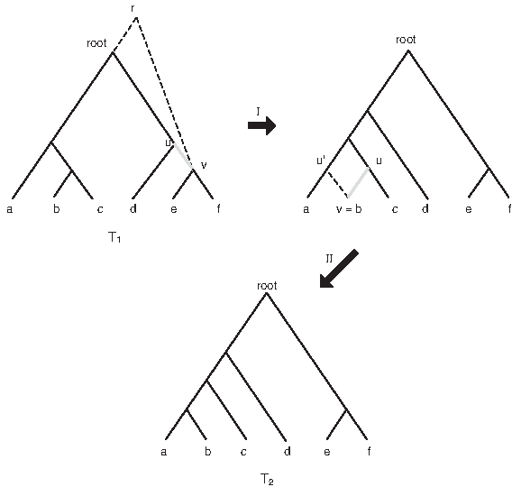
The tree T₁ undergoes two rSPR operations and is transformed into the tree T₂; the d_rSPR(T₁, T₂) = 2. The edges that are removed in the operations are showed in thick grey lines and the edges that are added are shown in dotted lines. In the first operation (I), the subtree restricted to {e, f} is the rSPR subtree and in the second (II), the subtree restricted to {b} is the rSPR subtree.

The d_rSPR distance

For trees T₁ and \documentclass{aastex}\usepackage{amsbsy}\usepackage{amsfonts}\usepackage{amssymb}\usepackage{bm}\usepackage{mathrsfs}\usepackage{pifont}\usepackage{stmaryrd}\usepackage{textcomp}\usepackage{portland,xspace}\usepackage{amsmath,amsxtra}\pagestyle{empty}\DeclareMathSizes{10}{9}{7}{6}\begin{document}$$T_2 \in B (X)$$\end{document} , the minimum number of rSPR operations that transform T₁ into T₂ is denoted by d_rSPR(T₁, T₂). Figure 2 shows a tree that undergoes two rSPR operations (see figure legend for explanation). Note that each of the rSPR operations is reversible, i.e., if T₂ can be transformed from T₁ by a rSPR operation with rSPR subtree S, the tree T₁ can be transformed from T₂ using a rSPR operation with S as the rSPR subtree. Thus, d_rSPR(T₁, T₂) = d_rSPR(T₂, T₁). We use this fact in our main algorithm, where we provide a sequence of operations that transform T₁ into T₂ by collecting some operations that transform T₁ into T₂ and some operations that transform T₂ and T₁. In fact, the d_rSPR is shown in Bordewich and Semple (2004) to be a distance metric. We use this fact in the appendix to show that a new distance metric that we will introduce in this section gives a lower bound for the d_rSPR distance.

Common and differing clusters between trees

For \documentclass{aastex}\usepackage{amsbsy}\usepackage{amsfonts}\usepackage{amssymb}\usepackage{bm}\usepackage{mathrsfs}\usepackage{pifont}\usepackage{stmaryrd}\usepackage{textcomp}\usepackage{portland,xspace}\usepackage{amsmath,amsxtra}\pagestyle{empty}\DeclareMathSizes{10}{9}{7}{6}\begin{document}$$T_1, T_2 \in B (X)$$\end{document} , the clusters that are present in both T₁ and T₂ are called common clusters in T₁ and T₂. We denote the set of all common clusters, including all singleton clusters, in T₁ and T₂ by C(T₁, T₂). The clusters that are present in T₁ but not in T₂ are called (T₁, T₂)-differing clusters in T₁. Recently, a distance measure called Cluster Index between T₁ and T₂, d_CI(T₁, T₂), has been defined in Restrepo et al. (2007) as the number of (T₁, T₂)-differing clusters in T₁, or equivalently in T₂. We note that this measure is related to the symmetric difference distance introduced by Robinson and Foulds (1981; for the definition, see Felsenstein, 2004), even though this has not been pointed out in Restrepo et al. (2007). To see the connection, add a dummy leaf with label “r” to each of T₁ and T₂, adjacent to their roots; then, the symmetric difference distance between the two resulting trees is the same as d_CI(T₁, T₂) (Fig. 3).

FIG. 3.

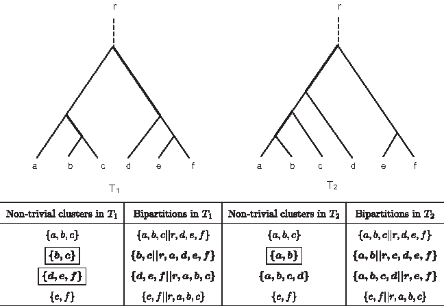
Two trees T₁ and T₂ with the same set of six leaf labels a − f. The non-trivial clusters of T₁ and T₂ are shown in the table. The clusters {a, b, c} and {e, f} are the same in both trees. All other non-trivial clusters are the (T₁, T₂)-differing clusters and (T₂, T₁)-differing clusters (shown in bold type). Cluster {a, b}, {b, c}. {d, e, f} (enclosed in boxes) are the (T₁, T₂) and (T₂, T₁)-minimal differing clusters. There are two (T₁, T₂)-differing clusters, hence d_CI(T₁, T₂) = 2. Also shown in the table are the bipartitions of the leaf set {r, a, b, c, d, e, f} obtained as a result of removing different edges in the tree. The symmetric difference between the trees is the number of bipartitions in one tree that is not in the other (shown in bold type). The edges that create the “differing” bipartitions are highlighted in bold in the trees. Each bipartition is listed by the side of the non-trivial cluster which forms a part of the bipartition. With this correspondence, we notice the conceptual similarity of the symmetric difference distance and the d_CI distance. There are two (T₁, T₂)-minimal differing clusters and one (T₂, T₁)-minimal differing cluster hence d_PCI(T₁, T₂) = max{2, 1} = 2.

Minimal differing clusters between trees

A minimal (T₁, T₂)-differing cluster is a (T₁, T₂)-differing cluster in T₁ that does not contain any other (T₁, T₂)-differing cluster. Figure 3 shows two trees and the differing and minimal differing clusters between them.

We use minimal differing clusters between T₁ and T₂ in our main algorithm. We also define a new distance measure that counts the minimal differing clusters between trees. For {i,j} = {1,2}, let MDC(T_i, T_j) be the set of all minimal (T₁, T₂)-differing clusters. Let \documentclass{aastex}\usepackage{amsbsy}\usepackage{amsfonts}\usepackage{amssymb}\usepackage{bm}\usepackage{mathrsfs}\usepackage{pifont}\usepackage{stmaryrd}\usepackage{textcomp}\usepackage{portland,xspace}\usepackage{amsmath,amsxtra}\pagestyle{empty}\DeclareMathSizes{10}{9}{7}{6}\begin{document}$$m(T_i, T_j) = \mid MDC_Ti(T_i, T_j) \mid$$\end{document} (the number of minimal (T₁, T₂)-differing clusters in T_i). We define the partial cluster index between T₁ and T₂ as d_PCI(T₁, T₂) : = max{m(T₁, T₂), m(T₂, T₁)} (Fig. 3).

We first prove that d_PCI satisfies the mathematical conditions to be called a metric. We use this fact to prove \documentclass{aastex}\usepackage{amsbsy}\usepackage{amsfonts}\usepackage{amssymb}\usepackage{bm}\usepackage{mathrsfs}\usepackage{pifont}\usepackage{stmaryrd}\usepackage{textcomp}\usepackage{portland,xspace}\usepackage{amsmath,amsxtra}\pagestyle{empty}\DeclareMathSizes{10}{9}{7}{6}\begin{document}$$\frac {d_{PCI} (T_1,T_2)} {2} \le \, {d_{rSPR}} (T_1,T_2).$$\end{document}

Lemma 1

d_PCI is a metric in the space of B(X).

Proof 1. To prove that d_PCI is a metric, we need to show that for \documentclass{aastex}\usepackage{amsbsy}\usepackage{amsfonts}\usepackage{amssymb}\usepackage{bm}\usepackage{mathrsfs}\usepackage{pifont}\usepackage{stmaryrd}\usepackage{textcomp}\usepackage{portland,xspace}\usepackage{amsmath,amsxtra}\pagestyle{empty}\DeclareMathSizes{10}{9}{7}{6}\begin{document}$$P, Q, R \in B (X)$$\end{document} , we have

(i) d_PCI(P, Q) ≥ 0 (non-negativity),

(ii) d_PCI(P, Q) = 0 if and only if P = Q (identity of indiscernibles),

(iii) d_PCI(P, Q) = d_PCI(Q, P) (symmetry),

(iv) d_PCI(P, R) ≤ d_PCI(P, Q) + d_PCI (Q, R) (triangle inequality).

*A cluster \documentclass{aastex}\usepackage{amsbsy}\usepackage{amsfonts}\usepackage{amssymb}\usepackage{bm}\usepackage{mathrsfs}\usepackage{pifont}\usepackage{stmaryrd}\usepackage{textcomp}\usepackage{portland,xspace}\usepackage{amsmath,amsxtra}\pagestyle{empty}\DeclareMathSizes{10}{9}{7}{6}\begin{document}$$C \in MDC \ (T_1, T_2)$$\end{document} if and only if C is a (T₁,T₂)-differing cluster in T₁ and any cluster \documentclass{aastex}\usepackage{amsbsy}\usepackage{amsfonts}\usepackage{amssymb}\usepackage{bm}\usepackage{mathrsfs}\usepackage{pifont}\usepackage{stmaryrd}\usepackage{textcomp}\usepackage{portland,xspace}\usepackage{amsmath,amsxtra}\pagestyle{empty}\DeclareMathSizes{10}{9}{7}{6}\begin{document}$$C^\prime \subset C$$\end{document} in T₁ or T₂ belongs to C(T₁, T₂).

This fact will be used throughout the proof for any possible pairs of trees \documentclass{aastex}\usepackage{amsbsy}\usepackage{amsfonts}\usepackage{amssymb}\usepackage{bm}\usepackage{mathrsfs}\usepackage{pifont}\usepackage{stmaryrd}\usepackage{textcomp}\usepackage{portland,xspace}\usepackage{amsmath,amsxtra}\pagestyle{empty}\DeclareMathSizes{10}{9}{7}{6}\begin{document}$$T_1, T_2 \in B (n)$$\end{document} .

(i): Since m(P, Q), m(P, Q) ≥ 0, we have \documentclass{aastex}\usepackage{amsbsy}\usepackage{amsfonts}\usepackage{amssymb}\usepackage{bm}\usepackage{mathrsfs}\usepackage{pifont}\usepackage{stmaryrd}\usepackage{textcomp}\usepackage{portland,xspace}\usepackage{amsmath,amsxtra}\pagestyle{empty}\DeclareMathSizes{10}{9}{7}{6}\begin{document}\begin{align*}d_{PCI} (P, Q) = \max \{m (P, Q), m (Q, P) \} \ge 0.\end{align*}\end{document}

(ii): MDC(P, Q) = φ and MDC(P, Q) = φ if and only if P and Q are identical; i.e., m(P, Q) = 0 and m(P, Q) = 0 if and only if P = Q.

(iii): Since \documentclass{aastex}\usepackage{amsbsy}\usepackage{amsfonts}\usepackage{amssymb}\usepackage{bm}\usepackage{mathrsfs}\usepackage{pifont}\usepackage{stmaryrd}\usepackage{textcomp}\usepackage{portland,xspace}\usepackage{amsmath,amsxtra}\pagestyle{empty}\DeclareMathSizes{10}{9}{7}{6}\begin{document}\begin{align*}\max \{m (P, Q), m (Q, P) \} \quad & = \quad \max \{m (Q, P), m (P, Q) \},\end{align*}\end{document}

we have \documentclass{aastex}\usepackage{amsbsy}\usepackage{amsfonts}\usepackage{amssymb}\usepackage{bm}\usepackage{mathrsfs}\usepackage{pifont}\usepackage{stmaryrd}\usepackage{textcomp}\usepackage{portland,xspace}\usepackage{amsmath,amsxtra}\pagestyle{empty}\DeclareMathSizes{10}{9}{7}{6}\begin{document}\begin{align*}d_{PCI} (P, Q) = d_{PCI} (Q, P).\end{align*}\end{document}

(iv): Without loss of generality, let d_PCI(P,R) = m(P,R). We will give an one-to-one function \documentclass{aastex}\usepackage{amsbsy}\usepackage{amsfonts}\usepackage{amssymb}\usepackage{bm}\usepackage{mathrsfs}\usepackage{pifont}\usepackage{stmaryrd}\usepackage{textcomp}\usepackage{portland,xspace}\usepackage{amsmath,amsxtra}\pagestyle{empty}\DeclareMathSizes{10}{9}{7}{6}\begin{document}$$\Phi: MDC (P, R) \rightarrow MDC (P, Q) \cup MDC (Q, R)$$\end{document} . This will show that \documentclass{aastex}\usepackage{amsbsy}\usepackage{amsfonts}\usepackage{amssymb}\usepackage{bm}\usepackage{mathrsfs}\usepackage{pifont}\usepackage{stmaryrd}\usepackage{textcomp}\usepackage{portland,xspace}\usepackage{amsmath,amsxtra}\pagestyle{empty}\DeclareMathSizes{10}{9}{7}{6}\begin{document}\begin{align*}d_{PCI} (P, R) \le d_{PCI} (P, Q) + d_{PCI} (Q, R)\end{align*}\end{document}

since \documentclass{aastex}\usepackage{amsbsy}\usepackage{amsfonts}\usepackage{amssymb}\usepackage{bm}\usepackage{mathrsfs}\usepackage{pifont}\usepackage{stmaryrd}\usepackage{textcomp}\usepackage{portland,xspace}\usepackage{amsmath,amsxtra}\pagestyle{empty}\DeclareMathSizes{10}{9}{7}{6}\begin{document}\begin{align*}d_{PCI} (P, R) \quad & = \quad \mid MDC (P, R) \mid \quad (by \ assumption), \\ \quad & \le \quad \mid MDC (P, Q) \cup MDC (Q, R) \mid \quad (by \ the \ one \hbox{-} to \hbox{-} one \ function \ \Phi),\end{align*}\end{document}

and since \documentclass{aastex}\usepackage{amsbsy}\usepackage{amsfonts}\usepackage{amssymb}\usepackage{bm}\usepackage{mathrsfs}\usepackage{pifont}\usepackage{stmaryrd}\usepackage{textcomp}\usepackage{portland,xspace}\usepackage{amsmath,amsxtra}\pagestyle{empty}\DeclareMathSizes{10}{9}{7}{6}\begin{document}$$MDC (P, Q) \cap MDC (Q, R) = \phi$$\end{document} (for, clusters in MDC(P, Q) are not in C(Q) and \documentclass{aastex}\usepackage{amsbsy}\usepackage{amsfonts}\usepackage{amssymb}\usepackage{bm}\usepackage{mathrsfs}\usepackage{pifont}\usepackage{stmaryrd}\usepackage{textcomp}\usepackage{portland,xspace}\usepackage{amsmath,amsxtra}\pagestyle{empty}\DeclareMathSizes{10}{9}{7}{6}\begin{document}$$MDC (Q, R) \subseteq C (Q))$$\end{document} ), \documentclass{aastex}\usepackage{amsbsy}\usepackage{amsfonts}\usepackage{amssymb}\usepackage{bm}\usepackage{mathrsfs}\usepackage{pifont}\usepackage{stmaryrd}\usepackage{textcomp}\usepackage{portland,xspace}\usepackage{amsmath,amsxtra}\pagestyle{empty}\DeclareMathSizes{10}{9}{7}{6}\begin{document}\begin{align*}\mid MDC (P, Q) \cup MDC (Q, R) \mid \quad & = \quad \mid MDC (P, Q) \mid + \mid MDC (Q, R) \mid \\ & = \quad m (P, Q) + m (Q, R) \\ & \le \quad d_{PCI} (P, Q) + d_{PCI} (Q, R).\end{align*}\end{document}

Let \documentclass{aastex}\usepackage{amsbsy}\usepackage{amsfonts}\usepackage{amssymb}\usepackage{bm}\usepackage{mathrsfs}\usepackage{pifont}\usepackage{stmaryrd}\usepackage{textcomp}\usepackage{portland,xspace}\usepackage{amsmath,amsxtra}\pagestyle{empty}\DeclareMathSizes{10}{9}{7}{6}\begin{document}$$C \in MDC_P (P, R)$$\end{document} , therefore \documentclass{aastex}\usepackage{amsbsy}\usepackage{amsfonts}\usepackage{amssymb}\usepackage{bm}\usepackage{mathrsfs}\usepackage{pifont}\usepackage{stmaryrd}\usepackage{textcomp}\usepackage{portland,xspace}\usepackage{amsmath,amsxtra}\pagestyle{empty}\DeclareMathSizes{10}{9}{7}{6}\begin{document}$$C \not \in C (R)$$\end{document} . We now define Φ(C) and prove that the Φ is a one-to-one function.

Case (a): Suppose \documentclass{aastex}\usepackage{amsbsy}\usepackage{amsfonts}\usepackage{amssymb}\usepackage{bm}\usepackage{mathrsfs}\usepackage{pifont}\usepackage{stmaryrd}\usepackage{textcomp}\usepackage{portland,xspace}\usepackage{amsmath,amsxtra}\pagestyle{empty}\DeclareMathSizes{10}{9}{7}{6}\begin{document}$$C \not \in C (Q)$$\end{document} . Let \documentclass{aastex}\usepackage{amsbsy}\usepackage{amsfonts}\usepackage{amssymb}\usepackage{bm}\usepackage{mathrsfs}\usepackage{pifont}\usepackage{stmaryrd}\usepackage{textcomp}\usepackage{portland,xspace}\usepackage{amsmath,amsxtra}\pagestyle{empty}\DeclareMathSizes{10}{9}{7}{6}\begin{document}$$C_P \in C (P)$$\end{document} be a cluster of minimal size such that \documentclass{aastex}\usepackage{amsbsy}\usepackage{amsfonts}\usepackage{amssymb}\usepackage{bm}\usepackage{mathrsfs}\usepackage{pifont}\usepackage{stmaryrd}\usepackage{textcomp}\usepackage{portland,xspace}\usepackage{amsmath,amsxtra}\pagestyle{empty}\DeclareMathSizes{10}{9}{7}{6}\begin{document}$$C_P \subseteq C$$\end{document} and \documentclass{aastex}\usepackage{amsbsy}\usepackage{amsfonts}\usepackage{amssymb}\usepackage{bm}\usepackage{mathrsfs}\usepackage{pifont}\usepackage{stmaryrd}\usepackage{textcomp}\usepackage{portland,xspace}\usepackage{amsmath,amsxtra}\pagestyle{empty}\DeclareMathSizes{10}{9}{7}{6}\begin{document}$$C_P \not \in C (Q)$$\end{document} ; it is possible that C_P = C.

Subcase (i): If \documentclass{aastex}\usepackage{amsbsy}\usepackage{amsfonts}\usepackage{amssymb}\usepackage{bm}\usepackage{mathrsfs}\usepackage{pifont}\usepackage{stmaryrd}\usepackage{textcomp}\usepackage{portland,xspace}\usepackage{amsmath,amsxtra}\pagestyle{empty}\DeclareMathSizes{10}{9}{7}{6}\begin{document}$$C_P \in MDC (P, Q)$$\end{document} , let Φ(C) = C_P.

Subcase (ii): If \documentclass{aastex}\usepackage{amsbsy}\usepackage{amsfonts}\usepackage{amssymb}\usepackage{bm}\usepackage{mathrsfs}\usepackage{pifont}\usepackage{stmaryrd}\usepackage{textcomp}\usepackage{portland,xspace}\usepackage{amsmath,amsxtra}\pagestyle{empty}\DeclareMathSizes{10}{9}{7}{6}\begin{document}$$C_P \not \in MDC (P, Q)$$\end{document} , by the minimality of C_P, there exists a \documentclass{aastex}\usepackage{amsbsy}\usepackage{amsfonts}\usepackage{amssymb}\usepackage{bm}\usepackage{mathrsfs}\usepackage{pifont}\usepackage{stmaryrd}\usepackage{textcomp}\usepackage{portland,xspace}\usepackage{amsmath,amsxtra}\pagestyle{empty}\DeclareMathSizes{10}{9}{7}{6}\begin{document}$$C_Q \in C (Q)$$\end{document} such that \documentclass{aastex}\usepackage{amsbsy}\usepackage{amsfonts}\usepackage{amssymb}\usepackage{bm}\usepackage{mathrsfs}\usepackage{pifont}\usepackage{stmaryrd}\usepackage{textcomp}\usepackage{portland,xspace}\usepackage{amsmath,amsxtra}\pagestyle{empty}\DeclareMathSizes{10}{9}{7}{6}\begin{document}$$C_Q \subset C_P$$\end{document} and \documentclass{aastex}\usepackage{amsbsy}\usepackage{amsfonts}\usepackage{amssymb}\usepackage{bm}\usepackage{mathrsfs}\usepackage{pifont}\usepackage{stmaryrd}\usepackage{textcomp}\usepackage{portland,xspace}\usepackage{amsmath,amsxtra}\pagestyle{empty}\DeclareMathSizes{10}{9}{7}{6}\begin{document}$$C_Q \not \in C (P)$$\end{document} . Choose C_Q to be a cluster of minimal size. The following reasonings prove that \documentclass{aastex}\usepackage{amsbsy}\usepackage{amsfonts}\usepackage{amssymb}\usepackage{bm}\usepackage{mathrsfs}\usepackage{pifont}\usepackage{stmaryrd}\usepackage{textcomp}\usepackage{portland,xspace}\usepackage{amsmath,amsxtra}\pagestyle{empty}\DeclareMathSizes{10}{9}{7}{6}\begin{document}$$C_Q \in MDC (Q, R)$$\end{document} :

1. Suppose \documentclass{aastex}\usepackage{amsbsy}\usepackage{amsfonts}\usepackage{amssymb}\usepackage{bm}\usepackage{mathrsfs}\usepackage{pifont}\usepackage{stmaryrd}\usepackage{textcomp}\usepackage{portland,xspace}\usepackage{amsmath,amsxtra}\pagestyle{empty}\DeclareMathSizes{10}{9}{7}{6}\begin{document}$$C^\prime \in C(R)$$\end{document} such that \documentclass{aastex}\usepackage{amsbsy}\usepackage{amsfonts}\usepackage{amssymb}\usepackage{bm}\usepackage{mathrsfs}\usepackage{pifont}\usepackage{stmaryrd}\usepackage{textcomp}\usepackage{portland,xspace}\usepackage{amsmath,amsxtra}\pagestyle{empty}\DeclareMathSizes{10}{9}{7}{6}\begin{document}$$C^\prime \subset C_Q$$\end{document} and \documentclass{aastex}\usepackage{amsbsy}\usepackage{amsfonts}\usepackage{amssymb}\usepackage{bm}\usepackage{mathrsfs}\usepackage{pifont}\usepackage{stmaryrd}\usepackage{textcomp}\usepackage{portland,xspace}\usepackage{amsmath,amsxtra}\pagestyle{empty}\DeclareMathSizes{10}{9}{7}{6}\begin{document}$$C^\prime \not \in C (Q)$$\end{document} . Since \documentclass{aastex}\usepackage{amsbsy}\usepackage{amsfonts}\usepackage{amssymb}\usepackage{bm}\usepackage{mathrsfs}\usepackage{pifont}\usepackage{stmaryrd}\usepackage{textcomp}\usepackage{portland,xspace}\usepackage{amsmath,amsxtra}\pagestyle{empty}\DeclareMathSizes{10}{9}{7}{6}\begin{document}$$C^\prime \subset C$$\end{document} , we have \documentclass{aastex}\usepackage{amsbsy}\usepackage{amsfonts}\usepackage{amssymb}\usepackage{bm}\usepackage{mathrsfs}\usepackage{pifont}\usepackage{stmaryrd}\usepackage{textcomp}\usepackage{portland,xspace}\usepackage{amsmath,amsxtra}\pagestyle{empty}\DeclareMathSizes{10}{9}{7}{6}\begin{document}$$C^\prime \in C (P)$$\end{document} . But \documentclass{aastex}\usepackage{amsbsy}\usepackage{amsfonts}\usepackage{amssymb}\usepackage{bm}\usepackage{mathrsfs}\usepackage{pifont}\usepackage{stmaryrd}\usepackage{textcomp}\usepackage{portland,xspace}\usepackage{amsmath,amsxtra}\pagestyle{empty}\DeclareMathSizes{10}{9}{7}{6}\begin{document}$$C^\prime \subset C_Q \subset C_P$$\end{document} and \documentclass{aastex}\usepackage{amsbsy}\usepackage{amsfonts}\usepackage{amssymb}\usepackage{bm}\usepackage{mathrsfs}\usepackage{pifont}\usepackage{stmaryrd}\usepackage{textcomp}\usepackage{portland,xspace}\usepackage{amsmath,amsxtra}\pagestyle{empty}\DeclareMathSizes{10}{9}{7}{6}\begin{document}$$C^\prime \not \in C (Q)$$\end{document} , a contradiction to the minimality of C_P.

2. Suppose \documentclass{aastex}\usepackage{amsbsy}\usepackage{amsfonts}\usepackage{amssymb}\usepackage{bm}\usepackage{mathrsfs}\usepackage{pifont}\usepackage{stmaryrd}\usepackage{textcomp}\usepackage{portland,xspace}\usepackage{amsmath,amsxtra}\pagestyle{empty}\DeclareMathSizes{10}{9}{7}{6}\begin{document}$$C^\prime \not \in C (Q)$$\end{document} such that \documentclass{aastex}\usepackage{amsbsy}\usepackage{amsfonts}\usepackage{amssymb}\usepackage{bm}\usepackage{mathrsfs}\usepackage{pifont}\usepackage{stmaryrd}\usepackage{textcomp}\usepackage{portland,xspace}\usepackage{amsmath,amsxtra}\pagestyle{empty}\DeclareMathSizes{10}{9}{7}{6}\begin{document}$$C^{\prime \prime} \subset C_Q$$\end{document} and \documentclass{aastex}\usepackage{amsbsy}\usepackage{amsfonts}\usepackage{amssymb}\usepackage{bm}\usepackage{mathrsfs}\usepackage{pifont}\usepackage{stmaryrd}\usepackage{textcomp}\usepackage{portland,xspace}\usepackage{amsmath,amsxtra}\pagestyle{empty}\DeclareMathSizes{10}{9}{7}{6}\begin{document}$$C^{\prime \prime} \not \in C (R)$$\end{document} . But by the minimality of C_Q, we have \documentclass{aastex}\usepackage{amsbsy}\usepackage{amsfonts}\usepackage{amssymb}\usepackage{bm}\usepackage{mathrsfs}\usepackage{pifont}\usepackage{stmaryrd}\usepackage{textcomp}\usepackage{portland,xspace}\usepackage{amsmath,amsxtra}\pagestyle{empty}\DeclareMathSizes{10}{9}{7}{6}\begin{document}$$C^{\prime \prime} \in C (P)$$\end{document} implying \documentclass{aastex}\usepackage{amsbsy}\usepackage{amsfonts}\usepackage{amssymb}\usepackage{bm}\usepackage{mathrsfs}\usepackage{pifont}\usepackage{stmaryrd}\usepackage{textcomp}\usepackage{portland,xspace}\usepackage{amsmath,amsxtra}\pagestyle{empty}\DeclareMathSizes{10}{9}{7}{6}\begin{document}$$C^{\prime \prime} \in C (R)$$\end{document} , a contradiction.

Thus \documentclass{aastex}\usepackage{amsbsy}\usepackage{amsfonts}\usepackage{amssymb}\usepackage{bm}\usepackage{mathrsfs}\usepackage{pifont}\usepackage{stmaryrd}\usepackage{textcomp}\usepackage{portland,xspace}\usepackage{amsmath,amsxtra}\pagestyle{empty}\DeclareMathSizes{10}{9}{7}{6}\begin{document}$$C_Q \in MDC (Q, R)$$\end{document} ; let Φ(C) = C_Q.

Case (b): Suppose \documentclass{aastex}\usepackage{amsbsy}\usepackage{amsfonts}\usepackage{amssymb}\usepackage{bm}\usepackage{mathrsfs}\usepackage{pifont}\usepackage{stmaryrd}\usepackage{textcomp}\usepackage{portland,xspace}\usepackage{amsmath,amsxtra}\pagestyle{empty}\DeclareMathSizes{10}{9}{7}{6}\begin{document}$$C \in C (Q)$$\end{document} .

Subcase (i): Suppose there exists \documentclass{aastex}\usepackage{amsbsy}\usepackage{amsfonts}\usepackage{amssymb}\usepackage{bm}\usepackage{mathrsfs}\usepackage{pifont}\usepackage{stmaryrd}\usepackage{textcomp}\usepackage{portland,xspace}\usepackage{amsmath,amsxtra}\pagestyle{empty}\DeclareMathSizes{10}{9}{7}{6}\begin{document}$$C_Q \in C (Q)$$\end{document} such that C_Q ⊂ C and \documentclass{aastex}\usepackage{amsbsy}\usepackage{amsfonts}\usepackage{amssymb}\usepackage{bm}\usepackage{mathrsfs}\usepackage{pifont}\usepackage{stmaryrd}\usepackage{textcomp}\usepackage{portland,xspace}\usepackage{amsmath,amsxtra}\pagestyle{empty}\DeclareMathSizes{10}{9}{7}{6}\begin{document}$$C_Q \not \in C (P)$$\end{document} . Choose C_Q of a minimal size. Suppose there exists \documentclass{aastex}\usepackage{amsbsy}\usepackage{amsfonts}\usepackage{amssymb}\usepackage{bm}\usepackage{mathrsfs}\usepackage{pifont}\usepackage{stmaryrd}\usepackage{textcomp}\usepackage{portland,xspace}\usepackage{amsmath,amsxtra}\pagestyle{empty}\DeclareMathSizes{10}{9}{7}{6}\begin{document}$$C_P \in C (P)$$\end{document} such that C_P ⊂ C_Q and \documentclass{aastex}\usepackage{amsbsy}\usepackage{amsfonts}\usepackage{amssymb}\usepackage{bm}\usepackage{mathrsfs}\usepackage{pifont}\usepackage{stmaryrd}\usepackage{textcomp}\usepackage{portland,xspace}\usepackage{amsmath,amsxtra}\pagestyle{empty}\DeclareMathSizes{10}{9}{7}{6}\begin{document}$$C_P \not \in C (Q)$$\end{document} . Choose C_P of minimal size. Then by the minimality of C_P and C_Q, we have \documentclass{aastex}\usepackage{amsbsy}\usepackage{amsfonts}\usepackage{amssymb}\usepackage{bm}\usepackage{mathrsfs}\usepackage{pifont}\usepackage{stmaryrd}\usepackage{textcomp}\usepackage{portland,xspace}\usepackage{amsmath,amsxtra}\pagestyle{empty}\DeclareMathSizes{10}{9}{7}{6}\begin{document}$$C_P \in MDC (P, Q)$$\end{document} ; let Φ(C) = C_P. Suppose there does not exist such a C_P, then \documentclass{aastex}\usepackage{amsbsy}\usepackage{amsfonts}\usepackage{amssymb}\usepackage{bm}\usepackage{mathrsfs}\usepackage{pifont}\usepackage{stmaryrd}\usepackage{textcomp}\usepackage{portland,xspace}\usepackage{amsmath,amsxtra}\pagestyle{empty}\DeclareMathSizes{10}{9}{7}{6}\begin{document}$$C_Q \in MDC (Q, R)$$\end{document} , since all clusters in R that are strictly contained in C_Q are clusters in P and therefore clusters in R, and all clusters in C(Q) are common in P and Q by the minimality of C_Q. Let Φ(C) = C_Q.

Subcase (ii): Suppose Subcase (i) does not hold but there exists \documentclass{aastex}\usepackage{amsbsy}\usepackage{amsfonts}\usepackage{amssymb}\usepackage{bm}\usepackage{mathrsfs}\usepackage{pifont}\usepackage{stmaryrd}\usepackage{textcomp}\usepackage{portland,xspace}\usepackage{amsmath,amsxtra}\pagestyle{empty}\DeclareMathSizes{10}{9}{7}{6}\begin{document}$$C_P \in C (P)$$\end{document} such that C_P ⊂ C and \documentclass{aastex}\usepackage{amsbsy}\usepackage{amsfonts}\usepackage{amssymb}\usepackage{bm}\usepackage{mathrsfs}\usepackage{pifont}\usepackage{stmaryrd}\usepackage{textcomp}\usepackage{portland,xspace}\usepackage{amsmath,amsxtra}\pagestyle{empty}\DeclareMathSizes{10}{9}{7}{6}\begin{document}$$C_P \not \in C (Q)$$\end{document} . Choose C_P minimal. Then \documentclass{aastex}\usepackage{amsbsy}\usepackage{amsfonts}\usepackage{amssymb}\usepackage{bm}\usepackage{mathrsfs}\usepackage{pifont}\usepackage{stmaryrd}\usepackage{textcomp}\usepackage{portland,xspace}\usepackage{amsmath,amsxtra}\pagestyle{empty}\DeclareMathSizes{10}{9}{7}{6}\begin{document}$$C_P \in MDC (P, Q)$$\end{document} ; let Φ(C) = C_P.

Subcase (iii): If the above two subcases do not hold, then \documentclass{aastex}\usepackage{amsbsy}\usepackage{amsfonts}\usepackage{amssymb}\usepackage{bm}\usepackage{mathrsfs}\usepackage{pifont}\usepackage{stmaryrd}\usepackage{textcomp}\usepackage{portland,xspace}\usepackage{amsmath,amsxtra}\pagestyle{empty}\DeclareMathSizes{10}{9}{7}{6}\begin{document}$$C \in MDC (Q, R)$$\end{document} since all clusters C′ ⊂ C such that \documentclass{aastex}\usepackage{amsbsy}\usepackage{amsfonts}\usepackage{amssymb}\usepackage{bm}\usepackage{mathrsfs}\usepackage{pifont}\usepackage{stmaryrd}\usepackage{textcomp}\usepackage{portland,xspace}\usepackage{amsmath,amsxtra}\pagestyle{empty}\DeclareMathSizes{10}{9}{7}{6}\begin{document}$$C^{\prime \prime} \in C (P)$$\end{document} satisfies \documentclass{aastex}\usepackage{amsbsy}\usepackage{amsfonts}\usepackage{amssymb}\usepackage{bm}\usepackage{mathrsfs}\usepackage{pifont}\usepackage{stmaryrd}\usepackage{textcomp}\usepackage{portland,xspace}\usepackage{amsmath,amsxtra}\pagestyle{empty}\DeclareMathSizes{10}{9}{7}{6}\begin{document}$$C^{\prime \prime} \in C (R)$$\end{document} , and all C″ ⊂ C(Q) such that \documentclass{aastex}\usepackage{amsbsy}\usepackage{amsfonts}\usepackage{amssymb}\usepackage{bm}\usepackage{mathrsfs}\usepackage{pifont}\usepackage{stmaryrd}\usepackage{textcomp}\usepackage{portland,xspace}\usepackage{amsmath,amsxtra}\pagestyle{empty}\DeclareMathSizes{10}{9}{7}{6}\begin{document}$$C^{\prime \prime} \in C (R)$$\end{document} satisfies \documentclass{aastex}\usepackage{amsbsy}\usepackage{amsfonts}\usepackage{amssymb}\usepackage{bm}\usepackage{mathrsfs}\usepackage{pifont}\usepackage{stmaryrd}\usepackage{textcomp}\usepackage{portland,xspace}\usepackage{amsmath,amsxtra}\pagestyle{empty}\DeclareMathSizes{10}{9}{7}{6}\begin{document}$$C^{\prime \prime} \in C (P)$$\end{document} and therefore \documentclass{aastex}\usepackage{amsbsy}\usepackage{amsfonts}\usepackage{amssymb}\usepackage{bm}\usepackage{mathrsfs}\usepackage{pifont}\usepackage{stmaryrd}\usepackage{textcomp}\usepackage{portland,xspace}\usepackage{amsmath,amsxtra}\pagestyle{empty}\DeclareMathSizes{10}{9}{7}{6}\begin{document}$$C^{\prime \prime} \in C (Q)$$\end{document} ; let Φ(C) = C.

Thus, for each \documentclass{aastex}\usepackage{amsbsy}\usepackage{amsfonts}\usepackage{amssymb}\usepackage{bm}\usepackage{mathrsfs}\usepackage{pifont}\usepackage{stmaryrd}\usepackage{textcomp}\usepackage{portland,xspace}\usepackage{amsmath,amsxtra}\pagestyle{empty}\DeclareMathSizes{10}{9}{7}{6}\begin{document}$$C \in MDC (P, Q)$$\end{document} , we have \documentclass{aastex}\usepackage{amsbsy}\usepackage{amsfonts}\usepackage{amssymb}\usepackage{bm}\usepackage{mathrsfs}\usepackage{pifont}\usepackage{stmaryrd}\usepackage{textcomp}\usepackage{portland,xspace}\usepackage{amsmath,amsxtra}\pagestyle{empty}\DeclareMathSizes{10}{9}{7}{6}\begin{document}\begin{align*}\Phi (C) \in MDC (P, Q) \cup MDC (Q, R).\end{align*}\end{document}

Moreover, \documentclass{aastex}\usepackage{amsbsy}\usepackage{amsfonts}\usepackage{amssymb}\usepackage{bm}\usepackage{mathrsfs}\usepackage{pifont}\usepackage{stmaryrd}\usepackage{textcomp}\usepackage{portland,xspace}\usepackage{amsmath,amsxtra}\pagestyle{empty}\DeclareMathSizes{10}{9}{7}{6}\begin{document}$$\Phi (C) \subseteq C$$\end{document} . Since all clusters in MDC(P, Q) are pairwise disjoint, we note that Φ is a one-to-one function, as required. ▪

Theorem 1

Let T₁ and \documentclass{aastex}\usepackage{amsbsy}\usepackage{amsfonts}\usepackage{amssymb}\usepackage{bm}\usepackage{mathrsfs}\usepackage{pifont}\usepackage{stmaryrd}\usepackage{textcomp}\usepackage{portland,xspace}\usepackage{amsmath,amsxtra}\pagestyle{empty}\DeclareMathSizes{10}{9}{7}{6}\begin{document}$$T_2 \in B (X)$$\end{document} . Then, \documentclass{aastex}\usepackage{amsbsy}\usepackage{amsfonts}\usepackage{amssymb}\usepackage{bm}\usepackage{mathrsfs}\usepackage{pifont}\usepackage{stmaryrd}\usepackage{textcomp}\usepackage{portland,xspace}\usepackage{amsmath,amsxtra}\pagestyle{empty}\DeclareMathSizes{10}{9}{7}{6}\begin{document}\begin{align*}\frac {d_{PCI} (T_1, T_2)} {2} \le d_{rSPR} (T_1, T_2).\end{align*}\end{document}

Proof 2 (Proof by induction). Let k be an integer such that d_rSPR(T₁, T₂) = k.

Suppose k = 1. In this proof, we identify the clusters using the labels specified to them. Figure 4 shows a pair of trees, T₁ and T₂ in which the labels A, B, C, D, X represent common clusters; and if all of A, B, C and D are non-empty, then A ∪ X, A ∪ X ∪ B and C ∪ D are (T₁, T₂)-differing clusters in T₁; and A ∪ B, X ∪ D and C ∪ X ∪ D are (T₁, T₂) clusters of T₂. We also assume that all clusters contained in each of A, B, C, D and X are also common to T₁ and T₂. Then d_rSPR(T₁, T₂) = 1, obtained by an rSPR operation with subtree corresponding to X as the rSPR subtree. To calculate d_PCI(T₁, T₂), consider the clusters in the trees that contain at least one of the clusters A, B, C and D. Note that at least two of A, B, C and D are non-empty, since if three or four of them are empty, then d_rSPR(T₁, T₂) = 0, a contradiction. By exhaustive enumeration, we see that d_PCI(T₁, T₂) = 2 if at least three of A, B, C and D are non-empty and d_PCI(T₁, T₂) = 1 if exactly two of them are non-empty. Thus d_PCI(T₁, T₂) = 1 or 2 if d_rSPR(T₁, T₂) = 1, and the result holds for this case.

FIG. 4.

This figure shows two trees T₁, T₂ with common clusters A, B, C, D and X; all clusters contained in each of them are also assumed to be common. Then d_rSPR(T₁, T₂) = 1 with the subtree corresponding to X as the rSPR subtree.

Now, let us assume that k > 1. There are k rSPR operations between T₁ to T₂ with trees \documentclass{aastex}\usepackage{amsbsy}\usepackage{amsfonts}\usepackage{amssymb}\usepackage{bm}\usepackage{mathrsfs}\usepackage{pifont}\usepackage{stmaryrd}\usepackage{textcomp}\usepackage{portland,xspace}\usepackage{amsmath,amsxtra}\pagestyle{empty}\DeclareMathSizes{10}{9}{7}{6}\begin{document}$$T_1 = S_0, S_1, S_2, \cdots, S_k = T_2$$\end{document} such that \documentclass{aastex}\usepackage{amsbsy}\usepackage{amsfonts}\usepackage{amssymb}\usepackage{bm}\usepackage{mathrsfs}\usepackage{pifont}\usepackage{stmaryrd}\usepackage{textcomp}\usepackage{portland,xspace}\usepackage{amsmath,amsxtra}\pagestyle{empty}\DeclareMathSizes{10}{9}{7}{6}\begin{document}$$d_{rSPR} (S_i, S_{i - 1}) = 1$$\end{document} . for \documentclass{aastex}\usepackage{amsbsy}\usepackage{amsfonts}\usepackage{amssymb}\usepackage{bm}\usepackage{mathrsfs}\usepackage{pifont}\usepackage{stmaryrd}\usepackage{textcomp}\usepackage{portland,xspace}\usepackage{amsmath,amsxtra}\pagestyle{empty}\DeclareMathSizes{10}{9}{7}{6}\begin{document}$$i = 1, 2, \cdots, k$$\end{document} Let us assume that the theorem holds for all tree pairs with d_rSPR less than k. Thus, \documentclass{aastex}\usepackage{amsbsy}\usepackage{amsfonts}\usepackage{amssymb}\usepackage{bm}\usepackage{mathrsfs}\usepackage{pifont}\usepackage{stmaryrd}\usepackage{textcomp}\usepackage{portland,xspace}\usepackage{amsmath,amsxtra}\pagestyle{empty}\DeclareMathSizes{10}{9}{7}{6}\begin{document}\begin{align*}d_{rSPR} (T_1, T_2) = d_{rSPR} (T_1, S_{k - 1}) + d_{rSPR} (S_{k - 1}, T_2), \tag{1}\end{align*}\end{document}

and by Lemma 1 , d_PCI satisfies the triangle inequality, and thus we have \documentclass{aastex}\usepackage{amsbsy}\usepackage{amsfonts}\usepackage{amssymb}\usepackage{bm}\usepackage{mathrsfs}\usepackage{pifont}\usepackage{stmaryrd}\usepackage{textcomp}\usepackage{portland,xspace}\usepackage{amsmath,amsxtra}\pagestyle{empty}\DeclareMathSizes{10}{9}{7}{6}\begin{document}\begin{align*}d_{PCI} (T_1, T_2) \quad & \le \quad d_{PCI} (T_1, S_{k - 1}) + d_{PCI} (S_{k - 1}, T_2) \\ & \le \quad 2 \bigg(\big(d_{rSPR} (T_1, S_{k - 1}) + d_{rSPR} (S_{k - 1}, T_2) \bigg) \quad \ by \ induction \ hypothesis, \\ & = \quad 2 d_{rSPR} (T_1, T_2) \quad by \ {(1)}.\end{align*}\end{document}

2.2. D-Clust: an algorithm to estimate the d_rSPR distance

In this section, we describe our algorithm D-Clust that finds the lower and the upper bounds for the d_rSPR distance and how it finds a sequence of rSPR operations that transform one tree into another.

D-Clust uses a result given by Bordewich and Semple (2004), which suggested an approximation algorithm. We now review this result and algorithm and then describe D-Clust, which improves the accuracy of that approximation.

Bordewich et al. proved that if \documentclass{aastex}\usepackage{amsbsy}\usepackage{amsfonts}\usepackage{amssymb}\usepackage{bm}\usepackage{mathrsfs}\usepackage{pifont}\usepackage{stmaryrd}\usepackage{textcomp}\usepackage{portland,xspace}\usepackage{amsmath,amsxtra}\pagestyle{empty}\DeclareMathSizes{10}{9}{7}{6}\begin{document}$$C \in C (T_1, T_2)$$\end{document} and \documentclass{aastex}\usepackage{amsbsy}\usepackage{amsfonts}\usepackage{amssymb}\usepackage{bm}\usepackage{mathrsfs}\usepackage{pifont}\usepackage{stmaryrd}\usepackage{textcomp}\usepackage{portland,xspace}\usepackage{amsmath,amsxtra}\pagestyle{empty}\DeclareMathSizes{10}{9}{7}{6}\begin{document}$$\overline{C} : \ = X - C$$\end{document} , then \documentclass{aastex}\usepackage{amsbsy}\usepackage{amsfonts}\usepackage{amssymb}\usepackage{bm}\usepackage{mathrsfs}\usepackage{pifont}\usepackage{stmaryrd}\usepackage{textcomp}\usepackage{portland,xspace}\usepackage{amsmath,amsxtra}\pagestyle{empty}\DeclareMathSizes{10}{9}{7}{6}\begin{document}\begin{align*}d_{rSPR} (T_1, T_2) \le d_{rSPR} (T_1 \mid C, T_2 \mid C) + d_{rSPR} (T_1 \mid \overline{C}, T_2 \mid \overline{C}) + 1 \le d_{rSPR} (T_1, T_2) + 1. \tag{2}\end{align*}\end{document}

The above set of inequalities suggests an algorithm that first chooses a common cluster C and breaks the problem into two sub-problems, one of which calculates \documentclass{aastex}\usepackage{amsbsy}\usepackage{amsfonts}\usepackage{amssymb}\usepackage{bm}\usepackage{mathrsfs}\usepackage{pifont}\usepackage{stmaryrd}\usepackage{textcomp}\usepackage{portland,xspace}\usepackage{amsmath,amsxtra}\pagestyle{empty}\DeclareMathSizes{10}{9}{7}{6}\begin{document}$$d_{rSPR} (T_1 \mid C, T_2 \mid C)$$\end{document} and the other calculates \documentclass{aastex}\usepackage{amsbsy}\usepackage{amsfonts}\usepackage{amssymb}\usepackage{bm}\usepackage{mathrsfs}\usepackage{pifont}\usepackage{stmaryrd}\usepackage{textcomp}\usepackage{portland,xspace}\usepackage{amsmath,amsxtra}\pagestyle{empty}\DeclareMathSizes{10}{9}{7}{6}\begin{document}$$d_{rSPR} (T_1 \mid \overline{C}, T_2 \mid \overline{C})$$\end{document} . The process can be repeated recursively until the sub-problems are reduced to calculating distances between identical trees. Since (2) is applied each time the problem subdivides, this procedure gives a lower bound and an upper bound for the distance, with the difference between the bounds equal to the number of subdivisions. The number of subdivisions can be minimized if the clusters with larger cardinalities are examined first, so that the smaller clusters are less likely to be considered for further subdivisions (since the recursive scheme stops at each largest cluster that induces identical subtrees in the trees, thus providing a narrow range between the bounds). We call this approach the APPROX-SPR algorithm. Interestingly, the algorithm RIATA-HGT (Nakhleh et al., 2005) can be seen as a version of APPROX-SPR, which includes, at each recursive step, an additional ingredient of using a set of leaves of maximum size that induce an identical subtree in the trees, in order to identify the transforming operations.

Choosing the common clusters is crucial to stop the recursion as early as possible, thus providing useful heuristics for the distance. In D-Clust, we make use of the minimal differing clusters to identify the appropriate common clusters. For this, we need some additional definitions. For \documentclass{aastex}\usepackage{amsbsy}\usepackage{amsfonts}\usepackage{amssymb}\usepackage{bm}\usepackage{mathrsfs}\usepackage{pifont}\usepackage{stmaryrd}\usepackage{textcomp}\usepackage{portland,xspace}\usepackage{amsmath,amsxtra}\pagestyle{empty}\DeclareMathSizes{10}{9}{7}{6}\begin{document}$$\{r, s \} = \{1, 2 \}$$\end{document} , we call a pair (C′, C″) with \documentclass{aastex}\usepackage{amsbsy}\usepackage{amsfonts}\usepackage{amssymb}\usepackage{bm}\usepackage{mathrsfs}\usepackage{pifont}\usepackage{stmaryrd}\usepackage{textcomp}\usepackage{portland,xspace}\usepackage{amsmath,amsxtra}\pagestyle{empty}\DeclareMathSizes{10}{9}{7}{6}\begin{document}$$C^\prime \in MDC({T_r},{T_s})$$\end{document} and \documentclass{aastex}\usepackage{amsbsy}\usepackage{amsfonts}\usepackage{amssymb}\usepackage{bm}\usepackage{mathrsfs}\usepackage{pifont}\usepackage{stmaryrd}\usepackage{textcomp}\usepackage{portland,xspace}\usepackage{amsmath,amsxtra}\pagestyle{empty}\DeclareMathSizes{10}{9}{7}{6}\begin{document}$$C^{\prime \prime} \in C (T_s)$$\end{document} , as a pair of nested clusters from {T₁, T₂} if \documentclass{aastex}\usepackage{amsbsy}\usepackage{amsfonts}\usepackage{amssymb}\usepackage{bm}\usepackage{mathrsfs}\usepackage{pifont}\usepackage{stmaryrd}\usepackage{textcomp}\usepackage{portland,xspace}\usepackage{amsmath,amsxtra}\pagestyle{empty}\DeclareMathSizes{10}{9}{7}{6}\begin{document}$$C^\prime \subset C^{\prime \prime}$$\end{document} . For a nested pair (C′, C″) of (T₁, T₂), the minimum number of common clusters \documentclass{aastex}\usepackage{amsbsy}\usepackage{amsfonts}\usepackage{amssymb}\usepackage{bm}\usepackage{mathrsfs}\usepackage{pifont}\usepackage{stmaryrd}\usepackage{textcomp}\usepackage{portland,xspace}\usepackage{amsmath,amsxtra}\pagestyle{empty}\DeclareMathSizes{10}{9}{7}{6}\begin{document}$$C_1, C_2, \cdots, C_k \in C (T_1, T_2)$$\end{document} such that \documentclass{aastex}\usepackage{amsbsy}\usepackage{amsfonts}\usepackage{amssymb}\usepackage{bm}\usepackage{mathrsfs}\usepackage{pifont}\usepackage{stmaryrd}\usepackage{textcomp}\usepackage{portland,xspace}\usepackage{amsmath,amsxtra}\pagestyle{empty}\DeclareMathSizes{10}{9}{7}{6}\begin{document}$$C^{\prime \prime} - C \prime = \cup_{i = 1}^k \ C_i$$\end{document} is denoted as d(C′, C″). In the Appendix, we show, using the equation (2), that if d(C′, C″) = k, for a positive integer k and \documentclass{aastex}\usepackage{amsbsy}\usepackage{amsfonts}\usepackage{amssymb}\usepackage{bm}\usepackage{mathrsfs}\usepackage{pifont}\usepackage{stmaryrd}\usepackage{textcomp}\usepackage{portland,xspace}\usepackage{amsmath,amsxtra}\pagestyle{empty}\DeclareMathSizes{10}{9}{7}{6}\begin{document}$$\overline{C} : \ = X - (C^{\prime \prime} - C^{\prime})$$\end{document} , then \documentclass{aastex}\usepackage{amsbsy}\usepackage{amsfonts}\usepackage{amssymb}\usepackage{bm}\usepackage{mathrsfs}\usepackage{pifont}\usepackage{stmaryrd}\usepackage{textcomp}\usepackage{portland,xspace}\usepackage{amsmath,amsxtra}\pagestyle{empty}\DeclareMathSizes{10}{9}{7}{6}\begin{document}\begin{align*}d_{rSPR} (T_1, T_2) - (k - 1) \quad & \le \quad \sum_{i = 1}^k d_{rSPR} (T_1 \mid C_i, T_2 \mid C_i) + d_{rSPR} (T_1 \mid \overline{C}, T_2 \mid \overline{C}) + 1 \\ & \le \quad d_{rSPR} (T_1, T_2). & (3)\end{align*}\end{document}

In other words, we have \documentclass{aastex}\usepackage{amsbsy}\usepackage{amsfonts}\usepackage{amssymb}\usepackage{bm}\usepackage{mathrsfs}\usepackage{pifont}\usepackage{stmaryrd}\usepackage{textcomp}\usepackage{portland,xspace}\usepackage{amsmath,amsxtra}\pagestyle{empty}\DeclareMathSizes{10}{9}{7}{6}\begin{document}\begin{align*}d_{rSPR} (T_1, T_2) \quad & \ge \quad \sum_{i = 1}^k d_{rSPR} (T_1 \mid C_i, T_2 \mid C_i) + d_{rSPR} (T_1 \mid \overline{C}, T_2 \mid \overline{C}) + 1, \rm{and} \\ d_{rSPR} (T_1, T_2) \quad & \le \quad \sum_{i = 1}^k d_{rSPR} (T_1 \mid C_i, T_2 \mid C_i) + d_{rSPR} (T_1 \mid \overline{C}, T_2 \mid \overline{C}) + k. & (4)\end{align*}\end{document}

The main idea in D-Clust consists of: first, finding a pair of nested clusters from {T₁, T₂} such that k = d(C′, C″) is minimized, and then subdividing the problem into k + 1 subproblems of finding each of \documentclass{aastex}\usepackage{amsbsy}\usepackage{amsfonts}\usepackage{amssymb}\usepackage{bm}\usepackage{mathrsfs}\usepackage{pifont}\usepackage{stmaryrd}\usepackage{textcomp}\usepackage{portland,xspace}\usepackage{amsmath,amsxtra}\pagestyle{empty}\DeclareMathSizes{10}{9}{7}{6}\begin{document}$$d_{rSPR} (T_1 \mid C_i, T_2 \mid C_i)$$\end{document} , for \documentclass{aastex}\usepackage{amsbsy}\usepackage{amsfonts}\usepackage{amssymb}\usepackage{bm}\usepackage{mathrsfs}\usepackage{pifont}\usepackage{stmaryrd}\usepackage{textcomp}\usepackage{portland,xspace}\usepackage{amsmath,amsxtra}\pagestyle{empty}\DeclareMathSizes{10}{9}{7}{6}\begin{document}$$i = 1, 2, \cdots, k$$\end{document} and \documentclass{aastex}\usepackage{amsbsy}\usepackage{amsfonts}\usepackage{amssymb}\usepackage{bm}\usepackage{mathrsfs}\usepackage{pifont}\usepackage{stmaryrd}\usepackage{textcomp}\usepackage{portland,xspace}\usepackage{amsmath,amsxtra}\pagestyle{empty}\DeclareMathSizes{10}{9}{7}{6}\begin{document}$$d_{rSPR} (T_1 \mid \overline{C}, T_2 \mid \overline{C})$$\end{document} . This process is continued recursively, with each step providing lower and upper bounds for the subdivision step. The lower and the upper bounds for d_rSPR(T₁, T₂) are respectively computed by adding the lower bounds and the upper bounds of each sub-problem. The pseudocode for D-Clust is given in Algorithm 1 below.

Algorithm 1. D-Clust(T₁, T₂)
Initialize LB : = 0,UB : = 0
Find C(T₁, T₂) and MDC_Ti(T₁, T₂) for \documentclass{aastex}\usepackage{amsbsy}\usepackage{amsfonts}\usepackage{amssymb}\usepackage{bm}\usepackage{mathrsfs}\usepackage{pifont}\usepackage{stmaryrd}\usepackage{textcomp}\usepackage{portland,xspace}\usepackage{amsmath,amsxtra}\pagestyle{empty}\DeclareMathSizes{10}{9}{7}{6}\begin{document}$$i \in \{1, 2 \}$$\end{document}
if T₁ and T₂ are identical then
return [LB, UB]
else
Choose a pair (C′, C″) of nested clusters from opposite trees (T₁, T₂) such that d(C′, C″) = k is minimum
\documentclass{aastex}\usepackage{amsbsy}\usepackage{amsfonts}\usepackage{amssymb}\usepackage{bm}\usepackage{mathrsfs}\usepackage{pifont}\usepackage{stmaryrd}\usepackage{textcomp}\usepackage{portland,xspace}\usepackage{amsmath,amsxtra}\pagestyle{empty}\DeclareMathSizes{10}{9}{7}{6}\begin{document}\begin{align}LB & = \textstyle\sum_{i = 1}^k {\rm D - Clust} (T_1 \mid C_i, T_2 \mid C_i) [LB] + {\rm D - Clust} (T_1 \mid \overline{C}, T_2 \mid \overline{C}) [LB] + 1 \\ UB & = \textstyle\sum_{i = 1}^k {\rm D - Clust} (T_1 \mid C_i, T_2 \mid C_i) [UB] + {\rm D - Clust} (T_1 \mid \overline{C}, T_2 \mid \overline{C}) [UB] + k\end{align}\end{document}
return [LB, UB]
end if

We now show that D-Clust is an extension of APPROX-SPR that narrows the range of values for the actual distance. We first note that the common clusters \documentclass{aastex}\usepackage{amsbsy}\usepackage{amsfonts}\usepackage{amssymb}\usepackage{bm}\usepackage{mathrsfs}\usepackage{pifont}\usepackage{stmaryrd}\usepackage{textcomp}\usepackage{portland,xspace}\usepackage{amsmath,amsxtra}\pagestyle{empty}\DeclareMathSizes{10}{9}{7}{6}\begin{document}$$C_i, i = 1, 2, \cdots, k$$\end{document} considered by D-Clust at each recursive step, are also considered for the subdivisions in APPROX-SPR. To observe this, notice that the smallest common cluster that contains \documentclass{aastex}\usepackage{amsbsy}\usepackage{amsfonts}\usepackage{amssymb}\usepackage{bm}\usepackage{mathrsfs}\usepackage{pifont}\usepackage{stmaryrd}\usepackage{textcomp}\usepackage{portland,xspace}\usepackage{amsmath,amsxtra}\pagestyle{empty}\DeclareMathSizes{10}{9}{7}{6}\begin{document}$$\cup_{i = 1}^k C_i$$\end{document} induces different subtrees in T₁ and T₂ (since the smallest common cluster must contain C′, which is differing between the trees; Fig. 4), and hence APPROX-SPR, through its recursive scheme will have to subdivide the problem for each of \documentclass{aastex}\usepackage{amsbsy}\usepackage{amsfonts}\usepackage{amssymb}\usepackage{bm}\usepackage{mathrsfs}\usepackage{pifont}\usepackage{stmaryrd}\usepackage{textcomp}\usepackage{portland,xspace}\usepackage{amsmath,amsxtra}\pagestyle{empty}\DeclareMathSizes{10}{9}{7}{6}\begin{document}$$C_i, i = 1, 2, \cdots, k$$\end{document} and \documentclass{aastex}\usepackage{amsbsy}\usepackage{amsfonts}\usepackage{amssymb}\usepackage{bm}\usepackage{mathrsfs}\usepackage{pifont}\usepackage{stmaryrd}\usepackage{textcomp}\usepackage{portland,xspace}\usepackage{amsmath,amsxtra}\pagestyle{empty}\DeclareMathSizes{10}{9}{7}{6}\begin{document}$$\overline{C}$$\end{document} . Secondly, note that these k + 1 subdivisions contribute a difference of k in APPROX-SPR, but by (3), only a difference of k − 1 in D-Clust.

Another useful implication of (2) has to do with the inference of the transforming rSPR operations. The inequalities in (2) suggest that a sequence of operations that transform T₁|C into T₂|C, combined with a sequence of operations that transform \documentclass{aastex}\usepackage{amsbsy}\usepackage{amsfonts}\usepackage{amssymb}\usepackage{bm}\usepackage{mathrsfs}\usepackage{pifont}\usepackage{stmaryrd}\usepackage{textcomp}\usepackage{portland,xspace}\usepackage{amsmath,amsxtra}\pagestyle{empty}\DeclareMathSizes{10}{9}{7}{6}\begin{document}$$T_1 \mid \overline{C}$$\end{document} into \documentclass{aastex}\usepackage{amsbsy}\usepackage{amsfonts}\usepackage{amssymb}\usepackage{bm}\usepackage{mathrsfs}\usepackage{pifont}\usepackage{stmaryrd}\usepackage{textcomp}\usepackage{portland,xspace}\usepackage{amsmath,amsxtra}\pagestyle{empty}\DeclareMathSizes{10}{9}{7}{6}\begin{document}$$T_2 \mid \overline{C}$$\end{document} transforms T₁ into T₂, along with possibly an extra operation with T|C as the rSPR tree. In D-Clust, we have a similar situation, where we can describe transforming rSPR operations at each recursive step and the set of all such operations can be compiled into a sequence of operations that transform T₁ into T₂. At each recursive step, D-Clust finds operations that collectively transform a subtree in T₁ into a subtree in T₂. An illustration of two trees with a pair of nested clusters is shown in Figure 5. Notice that k rSPR operations on T₁, each with \documentclass{aastex}\usepackage{amsbsy}\usepackage{amsfonts}\usepackage{amssymb}\usepackage{bm}\usepackage{mathrsfs}\usepackage{pifont}\usepackage{stmaryrd}\usepackage{textcomp}\usepackage{portland,xspace}\usepackage{amsmath,amsxtra}\pagestyle{empty}\DeclareMathSizes{10}{9}{7}{6}\begin{document}$$T_1 \mid C_i, i = 1, 2, \cdots, k$$\end{document} as the rSPR subtrees, transform the subtree \documentclass{aastex}\usepackage{amsbsy}\usepackage{amsfonts}\usepackage{amssymb}\usepackage{bm}\usepackage{mathrsfs}\usepackage{pifont}\usepackage{stmaryrd}\usepackage{textcomp}\usepackage{portland,xspace}\usepackage{amsmath,amsxtra}\pagestyle{empty}\DeclareMathSizes{10}{9}{7}{6}\begin{document}$$T_1 \mid C^{\prime \prime}$$\end{document} into \documentclass{aastex}\usepackage{amsbsy}\usepackage{amsfonts}\usepackage{amssymb}\usepackage{bm}\usepackage{mathrsfs}\usepackage{pifont}\usepackage{stmaryrd}\usepackage{textcomp}\usepackage{portland,xspace}\usepackage{amsmath,amsxtra}\pagestyle{empty}\DeclareMathSizes{10}{9}{7}{6}\begin{document}$$T_2 \mid C^{\prime \prime}$$\end{document} . We observe that these additional operations are those with \documentclass{aastex}\usepackage{amsbsy}\usepackage{amsfonts}\usepackage{amssymb}\usepackage{bm}\usepackage{mathrsfs}\usepackage{pifont}\usepackage{stmaryrd}\usepackage{textcomp}\usepackage{portland,xspace}\usepackage{amsmath,amsxtra}\pagestyle{empty}\DeclareMathSizes{10}{9}{7}{6}\begin{document}$$T \mid C_i, i = 1, 2, \cdots, k$$\end{document} as the subtrees. Furthermore, we can describe the operations as follows: Remove the subtree \documentclass{aastex}\usepackage{amsbsy}\usepackage{amsfonts}\usepackage{amssymb}\usepackage{bm}\usepackage{mathrsfs}\usepackage{pifont}\usepackage{stmaryrd}\usepackage{textcomp}\usepackage{portland,xspace}\usepackage{amsmath,amsxtra}\pagestyle{empty}\DeclareMathSizes{10}{9}{7}{6}\begin{document}$$T_r \mid C_i$$\end{document} from T_r and “regraft” it inside the subgraph induced by C′ to form a tree with the subtree identical to \documentclass{aastex}\usepackage{amsbsy}\usepackage{amsfonts}\usepackage{amssymb}\usepackage{bm}\usepackage{mathrsfs}\usepackage{pifont}\usepackage{stmaryrd}\usepackage{textcomp}\usepackage{portland,xspace}\usepackage{amsmath,amsxtra}\pagestyle{empty}\DeclareMathSizes{10}{9}{7}{6}\begin{document}$$T_s \mid C^{\prime \prime}$$\end{document} . The upper bound of d_rSPR in (4) corresponds to the number of operations that are involved in the subproblems in addition to the k operations described above.

FIG. 5.

In the top two trees (T₁ and T₂), x₁ and x₂ are two leaf labels and C₁,C₂ and C₃ are common clusters in T₁ and T₂. Thus, C′ : = {x₁, x₂} is a minimal differing cluster in T₁ and \documentclass{aastex}\usepackage{amsbsy}\usepackage{amsfonts}\usepackage{amssymb}\usepackage{bm}\usepackage{mathrsfs}\usepackage{pifont}\usepackage{stmaryrd}\usepackage{textcomp}\usepackage{portland,xspace}\usepackage{amsmath,amsxtra}\pagestyle{empty}\DeclareMathSizes{10}{9}{7}{6}\begin{document}$$C^{\prime \prime} : \ = \{x_1, x_2 \} \cup \cup_{i = 1}^kC_i$$\end{document} is a cluster in T₂. The tree at the bottom is obtained after applying 3 rSPR operations on T₁. Notice that these three operations are describable since they transform T₁|C″ into T₂|C″ by placing the subtrees \documentclass{aastex}\usepackage{amsbsy}\usepackage{amsfonts}\usepackage{amssymb}\usepackage{bm}\usepackage{mathrsfs}\usepackage{pifont}\usepackage{stmaryrd}\usepackage{textcomp}\usepackage{portland,xspace}\usepackage{amsmath,amsxtra}\pagestyle{empty}\DeclareMathSizes{10}{9}{7}{6}\begin{document}$$T_1 \mid C_i, i = 1, 2, \cdots, k$$\end{document} “inside” the subtree of T₁ induced by {x₁, x₂}.

In the Appendix, we discuss some implementation details and show that the algorithm runs in O(n⁴) time.

3. Experimental Results

3.1. Performance of D-Clust on tree-pairs with small d_rSPR distances

To test the accuracy of our algorithm, we generated synthetic datasets with specific d_rSPR distances. We first produced 100 random trees in B(n) for each of \documentclass{aastex}\usepackage{amsbsy}\usepackage{amsfonts}\usepackage{amssymb}\usepackage{bm}\usepackage{mathrsfs}\usepackage{pifont}\usepackage{stmaryrd}\usepackage{textcomp}\usepackage{portland,xspace}\usepackage{amsmath,amsxtra}\pagestyle{empty}\DeclareMathSizes{10}{9}{7}{6}\begin{document}$$n \in \{10, 20, \cdots, 110 \}$$\end{document} . For each of these trees T₀, we then produced trees T₁, T₂ and T₃ with d_rSPR(T₀, T_i) = i for i = 1, 2 and 3 by performing random rSPR operations. To generate T_i, we randomly applied i rSPR operations and then used the program SPRDist to verify the distances. In rare cases, SPRDist ran out of memory and did not output any estimates. For these cases, the lower and the upper bounds of our algorithm coincided, thus confirming the exact distance. We then ran the D-Clust algorithm for these pairs of trees. This approach may be extended to tree pairs with d_rSPR > 3. However, with the present implementation of SPRDist, the program crashed for at least 20% of the tree pairs with d_rSPR > 3, especially for trees with more than 30 leaves.

The upper and lower bounds of D-Clust were always equal to 1 for trees with distance 1. For distances 2 and 3, the picture was slightly more complicated. As can be seen from Table 1, the upper bound was typically near the exact distance, whereas the number of tree pairs for which D-Clust was able also to accurately estimate the lower bound, and therefore the exact distance, depended on the number of leaves in the tree and the actual distance. When the number of leaves was relatively small, the lower bound was lower than the actual value, but the bound abruptly became much tighter when the number of leaves increase to ∼50 or more. Thus, the ability of D-Clust to find the exact answer using the equality of the bounds depends on the ratio of the d_rSPR distance to the number of leaves, the lower the ratio the better is the accuracy.

Table 1.

For Each \documentclass{aastex}\usepackage{amsbsy}\usepackage{amsfonts}\usepackage{amssymb}\usepackage{bm}\usepackage{mathrsfs}\usepackage{pifont}\usepackage{stmaryrd}\usepackage{textcomp}\usepackage{portland,xspace}\usepackage{amsmath,amsxtra}\pagestyle{empty}\DeclareMathSizes{10}{9}{7}{6}\begin{document}$$n \in \{10, 20, \cdots, 110 \}$$\end{document} , the Table Shows the Percentage of Tree Pairs with Known d_rSPR Distances of 2 and 3, for which the Upper Bound of D-Clust Was Equal to the Exact Distances, and the Percentage of Tree Pairs for which the Lower and the Upper Bound Coincided

	SPR dist = 2		SPR dist = 3
N tips	% tree pairs with UB = 2	% tree pairs with UB = LB = 2	% tree pairs with UB = 3	% tree pairs with UB = LB = 3
10	99	78	98	37
20	100	98	96	77
30	100	95	98	90
40	100	96	98	94
50	100	95	100	97
60	100	98	99	97
70	100	100	100	97
80	99	98	100	96
90	100	98	100	97
100	100	100	100	99
110	100	98	100	97

Next, we considered the 320 benchmark tree pairs used in Hill et al. (2010) to compare the accuracy of the various algorithms. The dataset was formed by first taking a set of 320 trees and randomly performing certain specific number of rSPR operations on each of them. Tables 2 and 3 contain the results of D-Clust for these tree pairs. SPRDist was used to find the exact distance between the trees (not included) and for rare number of cases (∼10), D-Clust was used to confirm the exact distance. We noticed that the upper bounds of D-Clust match the exact distances for most tree pairs (310), consisting of all pairs with 50 or more leaves. With a very few (∼3) exceptions, a similar trend is followed by the lower bounds. For 382 pairs consisting of almost all the tree pairs with 50 or above leaves, the bounds coincided with the exact distance. Comparing these results with the results given in Hill et al. (2010) for the other algorithms, we conclude that the upper bounds given by D-Clust are close to the actual answer and the estimates given by the other heuristic algorithms; and in some cases, especially when the number of leaves and the distance are large, D-Clust gives the best solution. Furthermore, the lower bounds are equal to the upper bounds in such cases, thus providing the best results when other algorithms either give loose upper bounds and/or fail to compute the distance in reasonable space and time. D-Clust was able to compute the bounds on an average in ∼12 seconds and in less than 150 seconds for each tree pair, using less than 1 GB of RAM.

Table 2.

Results of D-Clust for 320 Tree Pairs

d_rSPR at most	No. of leaves	No. of pairs	Upper	Lower	Both
1	5	10	10	10	10
1	10	10	10	10	10
1	15	10	10	10	10
1	20	10	10	10	10
1	30	10	10	10	10
1	50	10	10	10	10
1	75	10	10	10	10
1	100	10	10	10	10
2	5	10	10	10	10
2	10	10	10	8 (1)	8
2	15	10	10	10	10
2	20	10	9 (2)	9 (1)	9
2	30	10	10	10	10
2	50	10	10	10	10
2	75	10	10	10	10
2	100	10	10	10	10
3	10	10	10	9 (1)	9

Each row presents the result for 10 tree pairs (third column) with the given number of leaves (second column), whose distance is at most the number given in the first column. The fourth column and the fifth column give the number of tree pairs for which the upper and lower bounds respectively of D-Clust matched the exact distance. Shown in the parenthesis in these columns average errors of the bounds for the tree pairs whose respective bounds did not match the exact distance. The sixth column shows the number of tree pairs whose lower and upper bounds both coincided with the exact distance. The contents of the table are continued in Table 3.

Table 3.

Continuation of Table 2

d_rSPR at most	No. of leaves	No. of pairs	Upper	Lower	Both
4	10	10	10	7 (1)	7
4	15	10	8 (1)	7 (1)	6
4	20	10	9 (1)	8 (1)	8
4	30	10	7 (2.6)	9 (1)	7
4	50	10	10	10	10
4	75	10	10	10	10
4	100	10	10	10	10
6	15	10	10	0 (1.3)	0
6	20	10	9 (3)	4 (1.3)	4
6	30	10	8 (4)	7 (2)	7
6	50	10	10	9 (1)	9
6	75	10	10	9 (1)	9
6	100	10	10	10	10
8	100	10	10	9 (1)	9
10	100	10	10	10	10
	Total		310	385	382

3.2. Performance of the bounds of D-Clust for random pairs of trees with unknown d_rSPR distances

In order to empirically determine the differences in values between the lower and upper bounds of D-Clust, we ran the algorithm for random tree pairs. Figure 6 shows the estimated values using both D-Clust and RIATA-HGT. We first observe that in general, the upper bound estimates of D-Clust are close to that of RIATA-HGT, with the estimates given by RIATA-HGT being slightly lower than that for D-Clust. In contrast, D-Clust outputs smaller upper bounds compared to RIATA-HGT for some trees pairs with large number of leaves and large distances between them (data not shown). Secondly, we observe that the lower bounds are very close to the upper bounds for trees with smaller number of leaves, and the upper bounds are about 7-fold larger than the lower bounds. From this, we conclude that D-Clust is currently most useful for computing the actual distance using equality of the bounds for relatively highly similar trees. On the other hand, RIATA-HGT and other approaches can find tight upper bounds efficiently, but are typically unable either to guarantee their solutions or to deliver the transforming operations. In order to improve the accuracy of the future approaches for large distances, it appears to be important to improve the lower bound.

FIG. 6.

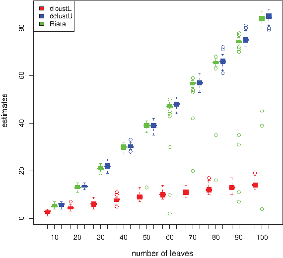
Box plot of the estimates by D-Clust and RIATA-HGT for 100 random pairs of trees for each \documentclass{aastex}\usepackage{amsbsy}\usepackage{amsfonts}\usepackage{amssymb}\usepackage{bm}\usepackage{mathrsfs}\usepackage{pifont}\usepackage{stmaryrd}\usepackage{textcomp}\usepackage{portland,xspace}\usepackage{amsmath,amsxtra}\pagestyle{empty}\DeclareMathSizes{10}{9}{7}{6}\begin{document}$$n \in \{10, 20, \cdots, 100 \}$$\end{document} (number of leaves).

4. Discussion

In this article, we gave a recursive algorithm D-Clust for the lower and upper bound heuristics for the NP-hard problem of computing the rSPR distance between trees. The algorithm runs in O(n⁴) time. We also provided empirical evidence that, in general, the upper bound is comparable to other upper bound heuristics, and that the lower and the upper bounds tend to coincide for the trees with small distances, with particularly good estimates for the trees with large number of leaves. Interestingly, a pair of trees with the large number of leaves and relatively small value of distance between the trees may model a common situation when a species tree and a gene tree, or two gene trees, are compared in search of a horizontal gene transfer event. Indeed, whereas the absolute number of the horizontal gene transfer events in the history of life may have been very large, the distribution of these events across the genomes and gene families may have been skewed, so that the vast majority of gene families appear to have experienced only a low rate of horizontal transfer (Lerat et al., 2005; Glazko et al., 2007; Molina and van Nimwegen, 2008). Thus, D-Clust may perform well for detecting horizontal gene transfer in the majority of gene/protein families. For large distances, the upper bounds are close to other upper bound heuristics, with large range of values between the bounds, suggesting that methods to compute better lower bound heuristics are desirable. Incorporating the D-Clust algorithm in any upper bound heuristic would provide a method for verifying the correctness of the heuristic and to improve the accuracy of calculating the exact distance. D-Clust also gives a sequence of rSPR operations that transform one tree into another tree which would be helpful in keeping track of the subtrees and the operations that are responsible for the differences between the trees.

A R program implementing the D-Clust algorithm is available upon request from one author (L.K.).

5. Appendix

5.1. Empirical distributions of the d_PCI, d_rSPR, and d_CI measures on random trees

The values of d_PCI, d_rSPR and d_CI measures between trees in B(X) all take values from 0 to n − 2, where n is the number of leaves in the trees. To obtain a more quantitative picture of the behavior of d_PCI, d_rSPR and d_CI, we compared these distances between simulated trees. We first generated 1000 pairs of trees with random topology in B(X) with |X| = 10 and calculated d_PCI, d_rSPR and d_CI between each pair of trees. Computing d_CI and d_PCI are straightforward, as they can be found easily by listing the clusters in each tree. To compute d_rSPR, we used the SPRDist program (Wu, 2009). Figure 7 shows the distribution of these distances for the 1000 tree pairs. The distributions of d_PCI and d_rSPR have similar shapes and ranges, with the peak of the former and the latter being, respectively, at 3 and 5, d_PCI being a lower bound for 2d_rSPR distance for any tree pair. In contrast, the distribution of the d_CI values is shifted towards larger values since it counts all differing clusters. A similar trend was observed on all tree pairs for a wide range of n up to 110 (data not shown).

FIG. 7.

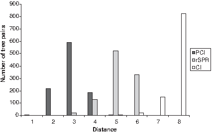
The frequency distributions of d_PCI, d_rSPR, and d_CI measures for 1000 random pairs of trees in B(X), with |X| = 10.

5.2. D-Clust: an algorithm that provides a lower bound and an upper bound for the d_rSPR distance

Given \documentclass{aastex}\usepackage{amsbsy}\usepackage{amsfonts}\usepackage{amssymb}\usepackage{bm}\usepackage{mathrsfs}\usepackage{pifont}\usepackage{stmaryrd}\usepackage{textcomp}\usepackage{portland,xspace}\usepackage{amsmath,amsxtra}\pagestyle{empty}\DeclareMathSizes{10}{9}{7}{6}\begin{document}$$T_1, T_2 \in B (x)$$\end{document} , D-Clust outputs a lower bound (LB) and an upper bound (UB) for the d_rSPR distance between T₁ and T₂.

We now prove the recursion that the algorithm uses. For \documentclass{aastex}\usepackage{amsbsy}\usepackage{amsfonts}\usepackage{amssymb}\usepackage{bm}\usepackage{mathrsfs}\usepackage{pifont}\usepackage{stmaryrd}\usepackage{textcomp}\usepackage{portland,xspace}\usepackage{amsmath,amsxtra}\pagestyle{empty}\DeclareMathSizes{10}{9}{7}{6}\begin{document}$$T \in B (n)$$\end{document} , the set of all leaf labels of T is denoted as L(T). For \documentclass{aastex}\usepackage{amsbsy}\usepackage{amsfonts}\usepackage{amssymb}\usepackage{bm}\usepackage{mathrsfs}\usepackage{pifont}\usepackage{stmaryrd}\usepackage{textcomp}\usepackage{portland,xspace}\usepackage{amsmath,amsxtra}\pagestyle{empty}\DeclareMathSizes{10}{9}{7}{6}\begin{document}$$C \subseteq L (T)$$\end{document} , the subtree of T that consists only C as its set of leaves is denoted as T|C.

Let \documentclass{aastex}\usepackage{amsbsy}\usepackage{amsfonts}\usepackage{amssymb}\usepackage{bm}\usepackage{mathrsfs}\usepackage{pifont}\usepackage{stmaryrd}\usepackage{textcomp}\usepackage{portland,xspace}\usepackage{amsmath,amsxtra}\pagestyle{empty}\DeclareMathSizes{10}{9}{7}{6}\begin{document}$$T_1, T_2 \in B (n)$$\end{document} . Let us assume that the roots of T₁ and T₂ are both labeled as ρ. An agreement forest for (T₁, T₂) is a collection \documentclass{aastex}\usepackage{amsbsy}\usepackage{amsfonts}\usepackage{amssymb}\usepackage{bm}\usepackage{mathrsfs}\usepackage{pifont}\usepackage{stmaryrd}\usepackage{textcomp}\usepackage{portland,xspace}\usepackage{amsmath,amsxtra}\pagestyle{empty}\DeclareMathSizes{10}{9}{7}{6}\begin{document}$$\{S_{\rho}, S_1, S_2, \cdots, S_k \}$$\end{document} , where S_ρ is a rooted tree and \documentclass{aastex}\usepackage{amsbsy}\usepackage{amsfonts}\usepackage{amssymb}\usepackage{bm}\usepackage{mathrsfs}\usepackage{pifont}\usepackage{stmaryrd}\usepackage{textcomp}\usepackage{portland,xspace}\usepackage{amsmath,amsxtra}\pagestyle{empty}\DeclareMathSizes{10}{9}{7}{6}\begin{document}$$S_1, S_2, \cdots, S_k$$\end{document} are rooted binary trees such that the following are satisfied:

(i) The leaf sets \documentclass{aastex}\usepackage{amsbsy}\usepackage{amsfonts}\usepackage{amssymb}\usepackage{bm}\usepackage{mathrsfs}\usepackage{pifont}\usepackage{stmaryrd}\usepackage{textcomp}\usepackage{portland,xspace}\usepackage{amsmath,amsxtra}\pagestyle{empty}\DeclareMathSizes{10}{9}{7}{6}\begin{document}$$L (S_{\rho}), L (S_1), L (S_2), \cdots, L (S_k)$$\end{document} partition L(T₁) ∪ {ρ} and in particular, \documentclass{aastex}\usepackage{amsbsy}\usepackage{amsfonts}\usepackage{amssymb}\usepackage{bm}\usepackage{mathrsfs}\usepackage{pifont}\usepackage{stmaryrd}\usepackage{textcomp}\usepackage{portland,xspace}\usepackage{amsmath,amsxtra}\pagestyle{empty}\DeclareMathSizes{10}{9}{7}{6}\begin{document}$$\rho \in L (S_{\rho})$$\end{document} .

(ii) For all \documentclass{aastex}\usepackage{amsbsy}\usepackage{amsfonts}\usepackage{amssymb}\usepackage{bm}\usepackage{mathrsfs}\usepackage{pifont}\usepackage{stmaryrd}\usepackage{textcomp}\usepackage{portland,xspace}\usepackage{amsmath,amsxtra}\pagestyle{empty}\DeclareMathSizes{10}{9}{7}{6}\begin{document}$$i \in \{\rho, 1, 2, \cdots, k \}$$\end{document} , S_i is isomorphic to T₁|L_i the subtree of T₁ and T₂ each of whose leaf set is L_i.

(iii) The trees in \documentclass{aastex}\usepackage{amsbsy}\usepackage{amsfonts}\usepackage{amssymb}\usepackage{bm}\usepackage{mathrsfs}\usepackage{pifont}\usepackage{stmaryrd}\usepackage{textcomp}\usepackage{portland,xspace}\usepackage{amsmath,amsxtra}\pagestyle{empty}\DeclareMathSizes{10}{9}{7}{6}\begin{document}$$\big \{T_1 \mid L_i : i \in \{\rho, 1, 2, \cdots, k \} \big \}$$\end{document} and \documentclass{aastex}\usepackage{amsbsy}\usepackage{amsfonts}\usepackage{amssymb}\usepackage{bm}\usepackage{mathrsfs}\usepackage{pifont}\usepackage{stmaryrd}\usepackage{textcomp}\usepackage{portland,xspace}\usepackage{amsmath,amsxtra}\pagestyle{empty}\DeclareMathSizes{10}{9}{7}{6}\begin{document}$$\big \{T_2 \mid L_i : i \in \{\rho, 1, 2, \cdots, k \} \big \}$$\end{document} are vertex-disjoint rooted subtrees of T₁ and T₂, respectively.

A maximum-agreement forest (MAF) of (T₁, T₂) is an agreement forest \documentclass{aastex}\usepackage{amsbsy}\usepackage{amsfonts}\usepackage{amssymb}\usepackage{bm}\usepackage{mathrsfs}\usepackage{pifont}\usepackage{stmaryrd}\usepackage{textcomp}\usepackage{portland,xspace}\usepackage{amsmath,amsxtra}\pagestyle{empty}\DeclareMathSizes{10}{9}{7}{6}\begin{document}$$\{S_{\rho}, S_1, S_2, \cdots, S_k \}$$\end{document} in which k is minimized. Hein (Hein et al., 1996) proved that the d_rSPR measure between two trees is one less than the number of trees in a MAF, i.e., d_rSPR(T₁, T₂) = k. In the results below, \documentclass{aastex}\usepackage{amsbsy}\usepackage{amsfonts}\usepackage{amssymb}\usepackage{bm}\usepackage{mathrsfs}\usepackage{pifont}\usepackage{stmaryrd}\usepackage{textcomp}\usepackage{portland,xspace}\usepackage{amsmath,amsxtra}\pagestyle{empty}\DeclareMathSizes{10}{9}{7}{6}\begin{document}$$\overline{C} : \ = X - C$$\end{document} .

Lemma 2

Let (C′, C″) be a pair of nested clusters from {T₁T₂} such that \documentclass{aastex}\usepackage{amsbsy}\usepackage{amsfonts}\usepackage{amssymb}\usepackage{bm}\usepackage{mathrsfs}\usepackage{pifont}\usepackage{stmaryrd}\usepackage{textcomp}\usepackage{portland,xspace}\usepackage{amsmath,amsxtra}\pagestyle{empty}\DeclareMathSizes{10}{9}{7}{6}\begin{document}$$C : \ = C^{\prime \prime} - C^{\prime} \in C (T_1, T_2)$$\end{document} Then, \documentclass{aastex}\usepackage{amsbsy}\usepackage{amsfonts}\usepackage{amssymb}\usepackage{bm}\usepackage{mathrsfs}\usepackage{pifont}\usepackage{stmaryrd}\usepackage{textcomp}\usepackage{portland,xspace}\usepackage{amsmath,amsxtra}\pagestyle{empty}\DeclareMathSizes{10}{9}{7}{6}\begin{document}\begin{align*}d_{rSPR} (T_1, T_2) = d_{rSPR} (T_1 \mid C, T_2 \mid C) + d_{rSPR} (T_1 \mid \overline{C}, T_2 \mid \overline{C}) + 1.\end{align*}\end{document}

Proof 3. By Bordewich and Semple (2004; Theorem 4.1), since C is a common cluster of T₁ and T₂, we have \documentclass{aastex}\usepackage{amsbsy}\usepackage{amsfonts}\usepackage{amssymb}\usepackage{bm}\usepackage{mathrsfs}\usepackage{pifont}\usepackage{stmaryrd}\usepackage{textcomp}\usepackage{portland,xspace}\usepackage{amsmath,amsxtra}\pagestyle{empty}\DeclareMathSizes{10}{9}{7}{6}\begin{document}\begin{align*}d_{rSPR} (T_1, T_2) \,\le \,d_{rSPR} (T_1 \mid C, T_2 \mid C) + d_{rSPR} (T_1 \mid \overline{C}, T_2 \mid \overline{C}) + 1 \le d_{rSPR} (T_1, T_2) + 1.\end{align*}\end{document}

Suppose the second inequality is an equality, then \documentclass{aastex}\usepackage{amsbsy}\usepackage{amsfonts}\usepackage{amssymb}\usepackage{bm}\usepackage{mathrsfs}\usepackage{pifont}\usepackage{stmaryrd}\usepackage{textcomp}\usepackage{portland,xspace}\usepackage{amsmath,amsxtra}\pagestyle{empty}\DeclareMathSizes{10}{9}{7}{6}\begin{document}\begin{align*}d_{rSPR} (T_1 \mid C, T_2 \mid C) + d_{rSPR} (T_1 \mid \overline{C}, T_2 \mid \overline{C}) = d_{rSPR} (T_1, T_2). \tag{5}\end{align*}\end{document}

Let us label the least common ancestor of C as ‘v’ in both T ₁ and T ₂ . Let \documentclass{aastex}\usepackage{amsbsy}\usepackage{amsfonts}\usepackage{amssymb}\usepackage{bm}\usepackage{mathrsfs}\usepackage{pifont}\usepackage{stmaryrd}\usepackage{textcomp}\usepackage{portland,xspace}\usepackage{amsmath,amsxtra}\pagestyle{empty}\DeclareMathSizes{10}{9}{7}{6}\begin{document}\begin{align*}{\cal F}_{\overline{C}} = \{S_{\rho}, S_1, S_2, \cdots, S_{k_1} \}\end{align*}\end{document}

be a MAF of \documentclass{aastex}\usepackage{amsbsy}\usepackage{amsfonts}\usepackage{amssymb}\usepackage{bm}\usepackage{mathrsfs}\usepackage{pifont}\usepackage{stmaryrd}\usepackage{textcomp}\usepackage{portland,xspace}\usepackage{amsmath,amsxtra}\pagestyle{empty}\DeclareMathSizes{10}{9}{7}{6}\begin{document}$$(T_1 \mid \overline{C}, T_2 \mid \overline{C})$$\end{document} , and let \documentclass{aastex}\usepackage{amsbsy}\usepackage{amsfonts}\usepackage{amssymb}\usepackage{bm}\usepackage{mathrsfs}\usepackage{pifont}\usepackage{stmaryrd}\usepackage{textcomp}\usepackage{portland,xspace}\usepackage{amsmath,amsxtra}\pagestyle{empty}\DeclareMathSizes{10}{9}{7}{6}\begin{document}\begin{align*}{\cal F}_C = \{S^{\prime}_v, S^{\prime}_1, S \prime_2, \cdots, S^{\prime}_{k_2} \}\end{align*}\end{document}

be a MAF of (T₁|C, T₂|C). By (5), there exists a \documentclass{aastex}\usepackage{amsbsy}\usepackage{amsfonts}\usepackage{amssymb}\usepackage{bm}\usepackage{mathrsfs}\usepackage{pifont}\usepackage{stmaryrd}\usepackage{textcomp}\usepackage{portland,xspace}\usepackage{amsmath,amsxtra}\pagestyle{empty}\DeclareMathSizes{10}{9}{7}{6}\begin{document}$$a \ i_0 \in \{1, 2, \cdots, k_1 \}$$\end{document} such that \documentclass{aastex}\usepackage{amsbsy}\usepackage{amsfonts}\usepackage{amssymb}\usepackage{bm}\usepackage{mathrsfs}\usepackage{pifont}\usepackage{stmaryrd}\usepackage{textcomp}\usepackage{portland,xspace}\usepackage{amsmath,amsxtra}\pagestyle{empty}\DeclareMathSizes{10}{9}{7}{6}\begin{document}\begin{align*}\{S_{\rho}, S_1, \cdots, S_{i_0 - 1}, S_{i_0} \cup S^{\prime}_v, S_{i_0 + 1}, \cdots, S_{k_1}, S^{\prime}_1, S^{\prime}_2, \cdots S_{k_2} \}\end{align*}\end{document}

is a MAF of (T₁, T₂). Since the cluster C″ contains C in T_j and since C′ is a minimal differing cluster in T_i, we have \documentclass{aastex}\usepackage{amsbsy}\usepackage{amsfonts}\usepackage{amssymb}\usepackage{bm}\usepackage{mathrsfs}\usepackage{pifont}\usepackage{stmaryrd}\usepackage{textcomp}\usepackage{portland,xspace}\usepackage{amsmath,amsxtra}\pagestyle{empty}\DeclareMathSizes{10}{9}{7}{6}\begin{document}$$C \prime \subseteq L (S_{i_0})$$\end{document} . But since C′ is a differing cluster, we conclude that T₁|L(S_i) ∪ L(S′_v) is not isomorphic to T₂|L(S_i) ∪ L(S′_v), a contradiction. The contradiction proves the statement of the lemma.

Theorem 2

Let (C′, C″) be a pair of nested clusters from {T₁, T₂} such that \documentclass{aastex}\usepackage{amsbsy}\usepackage{amsfonts}\usepackage{amssymb}\usepackage{bm}\usepackage{mathrsfs}\usepackage{pifont}\usepackage{stmaryrd}\usepackage{textcomp}\usepackage{portland,xspace}\usepackage{amsmath,amsxtra}\pagestyle{empty}\DeclareMathSizes{10}{9}{7}{6}\begin{document}$$C : \ = C^{\prime \prime} - C^{\prime} = \cup_{i = 1}^k C_i$$\end{document} , where \documentclass{aastex}\usepackage{amsbsy}\usepackage{amsfonts}\usepackage{amssymb}\usepackage{bm}\usepackage{mathrsfs}\usepackage{pifont}\usepackage{stmaryrd}\usepackage{textcomp}\usepackage{portland,xspace}\usepackage{amsmath,amsxtra}\pagestyle{empty}\DeclareMathSizes{10}{9}{7}{6}\begin{document}$$C_i \in C (T_1, T_2)$$\end{document} . Then, \documentclass{aastex}\usepackage{amsbsy}\usepackage{amsfonts}\usepackage{amssymb}\usepackage{bm}\usepackage{mathrsfs}\usepackage{pifont}\usepackage{stmaryrd}\usepackage{textcomp}\usepackage{portland,xspace}\usepackage{amsmath,amsxtra}\pagestyle{empty}\DeclareMathSizes{10}{9}{7}{6}\begin{document}\begin{align*}d_{rSPR} (T_1, T_2) - (k - 1) \quad & \le \quad \sum_{i = 1}^k d_{rSPR} (T_1 \mid C_i, T_2 \mid C_i) + d_{rSPR} (T_1 \mid \overline{C}, T_2 \mid \overline{C}) + 1 \\ & \le \quad d_{rSPR} (T_1, T_2).\end{align*}\end{document}

Proof 4. If k = 1, the statement follows from Lemma 2. Therefore, let us assume that k > 1. By (Bordewich and Semple, 2004, Theorem 4.1), we have \documentclass{aastex}\usepackage{amsbsy}\usepackage{amsfonts}\usepackage{amssymb}\usepackage{bm}\usepackage{mathrsfs}\usepackage{pifont}\usepackage{stmaryrd}\usepackage{textcomp}\usepackage{portland,xspace}\usepackage{amsmath,amsxtra}\pagestyle{empty}\DeclareMathSizes{10}{9}{7}{6}\begin{document}\begin{align*}d_{rSPR} (T_1 \mid C_1, T_2 \mid C_1) + d_{rSPR} (T_1 \mid \overline{C_1}, T_2 \mid \overline{C_1}) \le d_{rSPR} (T_1, T_2). \tag{6}\end{align*}\end{document}

But, by induction hypothesis, we have \documentclass{aastex}\usepackage{amsbsy}\usepackage{amsfonts}\usepackage{amssymb}\usepackage{bm}\usepackage{mathrsfs}\usepackage{pifont}\usepackage{stmaryrd}\usepackage{textcomp}\usepackage{portland,xspace}\usepackage{amsmath,amsxtra}\pagestyle{empty}\DeclareMathSizes{10}{9}{7}{6}\begin{document}\begin{align*}d_{rSPR} (T_1 \mid \overline{C_1}, T_2 \mid \overline{C_1}) - (k - 2) \quad & \le \quad \sum_{i = 2}^k d_{rSPR} (T_1 \mid C_i, T_2 \mid C_i) + d_{rSPR} (T_1 \mid \overline{C}, T_2 \mid \overline{C}) + 1 \\ & \le \quad d_{rSPR} (T_1 \mid \overline{C_1}, T_2 \mid \overline{C_1}). & (7)\end{align*}\end{document}

Substituting the upper and lower bounds of \documentclass{aastex}\usepackage{amsbsy}\usepackage{amsfonts}\usepackage{amssymb}\usepackage{bm}\usepackage{mathrsfs}\usepackage{pifont}\usepackage{stmaryrd}\usepackage{textcomp}\usepackage{portland,xspace}\usepackage{amsmath,amsxtra}\pagestyle{empty}\DeclareMathSizes{10}{9}{7}{6}\begin{document}$$d_{rSPR} (T_1 \mid \overline{C_1}, T_2 \mid \overline{C_1})$$\end{document} in (7) in (6), we get the required result.

5.2.1. Time complexity

Below are some implementation details and a justification for the complexity of O(n⁴) for D-Clust.

The computationally intensive part in each recursive step in D-Clust is to find a pair (C′, C″) of nested clusters from opposite trees (T₁, T₂) such that d(C′, C″) = k is minimum. For this, we need to first find the differing and common clusters, second compute the minimal differing clusters, third list the nested clusters, fourth find the minimum number of common clusters in each pair of nested clusters. For this, we maintain a 3-dimensional array M. In other words, M is a matrix whose entries are lists of leaf labels. The row indices of M corresponds to the clusters of T₁ arranged in an increasing order of the cluster size and the column indices represents the clusters of T₂ arranged in increasing order of the cluster size, and the entries of M contains the set union of the two clusters corresponding to the row and column. Note that each entry of M can be computed in O(n) time and thus it takes O(n³) time to compute the entries of M.

To find the common clusters, it is enough to traverse the entries in M and see if the entries are equal to their corresponding column and row (takes, O(n²) time). The clusters that are not common are differing.

To find minimal differing clusters, the differing clusters are compared with the other clusters in both the trees, thus taking O(n³) time.

To find the nested pairs of clusters, the rows and columns corresponding to each minimal differing cluster C′ can be traversed to find a cluster C″ of minimum size in the opposite tree that contains the cluster. This takes O(n) time for each minimal differing cluster if the lengths of the entries of M are also stored. Since the number of minimal differing clusters is O(n), finding all nested pairs has a complexity of O(n²).

To find the minimum k, for each nested pair (C′, C″ it is enough to traverse the row or column in M corresponding to C″ in the reverse order (bigger common cluster to smaller) to find the common clusters \documentclass{aastex}\usepackage{amsbsy}\usepackage{amsfonts}\usepackage{amssymb}\usepackage{bm}\usepackage{mathrsfs}\usepackage{pifont}\usepackage{stmaryrd}\usepackage{textcomp}\usepackage{portland,xspace}\usepackage{amsmath,amsxtra}\pagestyle{empty}\DeclareMathSizes{10}{9}{7}{6}\begin{document}$$C_1, C_2, \cdots, C_k$$\end{document} such that ∪C_i = C″ − C′. Since the total number of nested pairs is O(n), finding minimum k takes O(n³) time.

Thus, each recursive step has a complexity of O(n³). Since there can be be at most n recursive steps, the complexity of D-Clust is O(n⁴).

An implementation of D-Clust in R can be found at http://sourceforge.net/projects/dclust.

Footnotes

Acknowledgment

We thank Boris Rubinstein for critical reading of this manuscript.

Disclosure Statement

No competing financial interests exist.

References

Baroni

, Grunewald

, Moulton

et al. 2005. Bounding the number of hybridisation events for a consistent evolutionary history. J. Math. Biol., 51:171–182.

Beiko

R.G.

, Hamilton

2006. Phylogenetic identification of lateral genetic transfer events. BMC Evol. Biol., 6:15.

Bordewich

, Semple

2004. On the computational complexity of the rooted subtree prune and regraft distance. Ann. Combin., 8:409–423.

Clauset

, Moore

, Newman

M.E.

2008. Hierarchical structure and the prediction of missing links in networks. Nature, 453:98–101.

Robinson

D.F.

, Foulds

L.R.

1981. Comparison of phylogenetic trees. Math. Biosci., 53:131–147.

Diestel

2005. Graph Theory. Graduate Texts in Mathematics, 173 3rd. Springer: Berlin.

Felsenstein

2004. Inferring Phylogenies. Sinauer Associates Inc.: Sunderland, MA.

Glazko

, Makarenkov

, Liu

et al. 2007. Evolutionary history of bacteriophages with double-stranded dna genomes. Biol. Direct, 2:36.

Goloboff

P.A.

2007. Calculating spr distances between trees. Cladistics, 24:591–697.

10.

Hallett

M.T.

, Lagergren

2001. Efficient algorithms for lateral gene transfer problems. Proc. 5th Annu. Inte. Conf. Comput. Biol, 149–156.

11.

Hein

1990. Reconstructing evolution of sequences subject to recombination using parsimony. Math Biosci., 98:185–200.

12.

Hein

, Jiang

, Wang

et al. 1996. On the complexity of comparing evolutionary trees. Discrete Appl. Math., 71:153–169.

13.

Hill

, Nordstrom

K.J.

, Thollesson

et al. 2010. Sprit: identifying horizontal gene transfer in rooted phylogenetic trees. BMC Evol. Biol., 10:42.

14.

Lerat

, Daubin

, Ochman

et al. 2005. Evolutionary origins of genomic repertoires in bacteria. PLoS Biol., 3:e130.

15.

MacLeod

, Charlebois

R.L.

, Doolittle

et al. 2005. Deduction of probable events of lateral gene transfer through comparison of phylogenetic trees by recursive consolidation and rearrangement. BMC Evol. Biol., 5:27.

16.

Molina

, van Nimwegen

2008. The evolution of domain-content in bacterial genomes. Biol. Direct, 3:51.

17.

Nakhleh

, Ruths

, Wang

L.-S.

2005. RIATA-HGT: a fast and accurate heuristic for reconstructing horizontal gene transfer. Lect. Notes Comput. Sci., 3595:84–93.

18.

Restrepo

, Mesa

, Llanos

E.J.

2007. Three dissimilarity measures to contrast dendrograms. J. Chem. Inf. Model., 47:761–770.

19.

Song

Y.S.

, Hein

2005. Constructing minimal ancestral recombination graphs. J. Comput. Biol., 12:147–169.

20.

Than

, Ruths

, Nakhleh

2008. Phylonet: a software package for analyzing and reconstructing reticulate evolutionary relationships. BMC Bioinform., 9:322.

21.

Wang

, Zhang

2001. Perfect phylogenetic networks with recombination. J. Comput. Biol., 8:69–78.

22.

2009. A practical method for exact computation of subtree prune and regraft distance. Bioinformatics, 25:190–196.

A Polynomial-Time Algorithm Computing Lower and Upper Bounds of the Rooted Subtree Prune and Regraft Distance

Abstract

Abstract

1. Introduction

2. Methods

2.1. Definitions

Descendant and ancestor of a vertex in T

Subtrees of a tree rooted at a vertex

Clusters in a tree

Subtree of a tree induced by a leaf set

SPR operation on a tree

The drSPR distance

Common and differing clusters between trees

Minimal differing clusters between trees

Lemma 1

Theorem 1

2.2. D-Clust: an algorithm to estimate the drSPR distance

3. Experimental Results

3.1. Performance of D-Clust on tree-pairs with small drSPR distances

3.2. Performance of the bounds of D-Clust for random pairs of trees with unknown drSPR distances

4. Discussion

5. Appendix

5.1. Empirical distributions of the dPCI, drSPR, and dCI measures on random trees

5.2. D-Clust: an algorithm that provides a lower bound and an upper bound for the drSPR distance

Lemma 2

Theorem 2

5.2.1. Time complexity

Footnotes

Acknowledgment

Disclosure Statement

References

The d_rSPR distance

2.2. D-Clust: an algorithm to estimate the d_rSPR distance

3.1. Performance of D-Clust on tree-pairs with small d_rSPR distances

3.2. Performance of the bounds of D-Clust for random pairs of trees with unknown d_rSPR distances

5.1. Empirical distributions of the d_PCI, d_rSPR, and d_CI measures on random trees

5.2. D-Clust: an algorithm that provides a lower bound and an upper bound for the d_rSPR distance