Estimating the weight of evidence in forensic genetics is often done in terms of a likelihood ratio, LR. The LR evaluates the probability of the observed evidence under competing hypotheses. Most often, probabilities used in the LR only consider the evidence from the genomic variation identified using polymorphic genetic markers. However, modern typing techniques supply additional quantitative data, which contain very important information about the observed evidence. This is particularly true for cases of DNA mixtures, where more than one individual has contributed to the observed biological stain. This article presents a method for including the quantitative information of short tandem repeat (STR) DNA mixtures in the LR. Also, an efficient algorithmic method for finding the best matching combination of DNA mixture profiles is derived and implemented in an on-line tool for two- and three-person DNA mixtures. Finally, we demonstrate for two-person mixtures how this best matching pair of profiles can be used in estimating the likelihood ratio using importance sampling. The reason for using importance sampling for estimating the likelihood ratio is the often vast number of combinations of profiles needed for the evaluation of the weight of evidence. Online tool is available at http://people.math.aau.dk/∼tvede/dna/.
1. Introduction
When a crime has been committed, biological traces are often found at the scene of the crime. In many cases, more than one individual has contributed to the stain, which is then considered a DNA mixture. The evaluation of DNA mixtures are often complex and laborious, taking experienced case workers lots of time and effort to analyze.
Most modern DNA typing techniques are based upon polymerase chain reaction (PCR) producing millions of copies of the DNA string. The amount of DNA in the PCR vessel pre-PCR is reflected in the concentration of target molecules post-PCR. The targets used in forensic genetics are selected such that they are highly polymorphic (large number of possible alleles), which gives a high power of discrimination. Furthermore, the genetic markers used for forensic purposes are non-coding and should ideally be neutral with respect to selection.
The prevalent technology used in forensic genetics to perform genetic identification uses short tandem repeat (STR) polymorphisms. This method relies on variability in the length of certain repeat motifs in the genome. The STR DNA profile is observed via a so-called electropherogram (EPG), where the alleles are identified as signal peaks above a signal to noise threshold (see Fig. 2 below). For a single person DNA profile, one can observe either one or two peaks referring to the situation, where the DNA profile is either homozygous (identical alleles on both chromosomes) or heterozygous (different alleles on each chromosome). The commercial kits used for identification purposes typically contain between 10 to 15 genetic markers (also called loci: plural for locus). Within each locus, the number of alleles varies from 5 to 20. For the kit (SGM Plus Kit, Applied Biosystems) depicted in Figure 2 below, the labels “D3”, “vWA,” … “FGA” refer to locus names, and the integer values above the locus name correspond to the observed allele types for that particular locus.
It is possible only to observe the cumulative peaks in the EPG. That is, the peak heights are expected to be twice the height for homozygous loci relative to the heterozygous loci, since the two identical alleles doubles the amount of pre-PCR product for the homozygous peaks. This is also true for DNA mixtures where alleles shared by two or more contributors will reflect the contribution from more donors as higher peaks. Hence, for DNA mixtures with two contributors, the number of observable peaks ranges from one to four alleles depending on the particular profiles in the mixture.
The kit used for STR typing comprises a set of loci,
\documentclass{aastex}
\usepackage{amsbsy}
\usepackage{amsfonts}
\usepackage{amssymb}
\usepackage{bm}
\usepackage{mathrsfs}
\usepackage{pifont}
\usepackage{stmaryrd}
\usepackage{textcomp}
\usepackage{portland, xspace}
\usepackage{amsmath, amsxtra}
\pagestyle{empty}
\DeclareMathSizes {10} {9} {7} {6}
\begin{document}
$${ \cal S}$$
\end{document}, used for discrimination. For an arbitrary two-person mixture, the number of possible combinations are given by
\documentclass{aastex}
\usepackage{amsbsy}
\usepackage{amsfonts}
\usepackage{amssymb}
\usepackage{bm}
\usepackage{mathrsfs}
\usepackage{pifont}
\usepackage{stmaryrd}
\usepackage{textcomp}
\usepackage{portland, xspace}
\usepackage{amsmath, amsxtra}
\pagestyle{empty}
\DeclareMathSizes {10} {9} {7} {6}
\begin{document}
$$1^{S_1}7^{S_2}12^{S_3}6^{S_4}$$
\end{document}, where Si is the number of loci with i observations and
\documentclass{aastex}
\usepackage{amsbsy}
\usepackage{amsfonts}
\usepackage{amssymb}
\usepackage{bm}
\usepackage{mathrsfs}
\usepackage{pifont}
\usepackage{stmaryrd}
\usepackage{textcomp}
\usepackage{portland, xspace}
\usepackage{amsmath, amsxtra}
\pagestyle{empty}
\DeclareMathSizes {10} {9} {7} {6}
\begin{document}
$$S = \sum \nolimits_{i = 1}^4 S_i$$
\end{document}, is the total number of loci used for discrimination, i.e., S is the size of
\documentclass{aastex}
\usepackage{amsbsy}
\usepackage{amsfonts}
\usepackage{amssymb}
\usepackage{bm}
\usepackage{mathrsfs}
\usepackage{pifont}
\usepackage{stmaryrd}
\usepackage{textcomp}
\usepackage{portland, xspace}
\usepackage{amsmath, amsxtra}
\pagestyle{empty}
\DeclareMathSizes {10} {9} {7} {6}
\begin{document}
$${ \cal S}$$
\end{document}. The numbers 1, 7, 12, and 6 comes from the number of possible combinations (Table 1) when observing 1, 2, 3, and 4 alleles, respectively.
Possible Combinations in a Two-Person Mixture with One to Four Alleles
Alleles
Possible combinations
a
(aa, aa)
a, b
(aa, ab)
(aa, bb)
(ab, aa)
(ab, ab)
(ab, bb)
(bb, ab)
(bb, aa)
a, b, c
(aa, bc)
(ab, ac)
(ab, bc)
(ab, cc)
(ac, ab)
(ac, bb)
(ac, bc)
(bb, ac)
(bc, ab)
(bc, ac)
(bc, aa)
(cc, ab)
a, b, c, d
(ab, cd)
(ac, bd)
(ad, bc)
(bc, ad)
(bd, ac)
(cd, ab)
In most cases, this leads to an intractable number of combinations. However, using the quantitative STR data (peak heights and peak areas), the number of plausible combinations often decreases substantially. In this article, we develop a statistical model for STR DNA mixtures. The statistical model is intended to measure the agreement between the expected peak intensities for a proposed combination of DNA profiles and the actual observed peak intensities. Hence, we use an objective criterion to discriminate among the possible combinations in Table 1.
In order to incorporate the peak intensities in the likelihood ratio (LR), we first demonstrate how to find a best matching pair of profiles for a given two-person mixture using an efficient algorithmic approach. This algorithm iteratively builds up a best matching combination of profiles using the statistical model for the peak intensities. The algorithm has been implemented in a free online tool available at the first author's website (http://people.math.aau.dk/∼tvede/dna/). The statistical model and algorithmic construction are different from previously proposed methods for DNA mixture separation (Perlin and Szabady, 2001; Wang et al., 2006).
The inclusion of the quantitative information in the LR is done by assigning a weight to each combination of DNA profiles consistent with the observed STR types. The weight reflects the probability of observing the observed peak intensities given a specific combination of profiles. The denominator in the LR will in most cases yield a sum over an intractable number of combination. By sampling “close” to the best matching combination returned by the algorithm, we show how importance sampling may be used to estimate the LR.
2. Data
The model is based on exploration of controlled experiments of two-person mixtures conducted at The Section of Forensic Genetics, Department of Forensic Medicine, Faculty of Health Sciences, University of Copenhagen, Denmark. From the data exploration, it is evident that the mean and covariance structure of the peak areas must satisfy proportionality of:
• peak areas and peak heights,
• peak area and amount of DNA in the mixture,
• the mean and variance of the peak areas.
These assumptions are supported elsewhere (Figs. 1 and 2 in Tvedebrink et al., 2010). The experiments consisted of pairwise two-person mixtures in various mixture ratios of the four profiles in Table 2. The data were prepared as described in Tvedebrink et al. (2009).
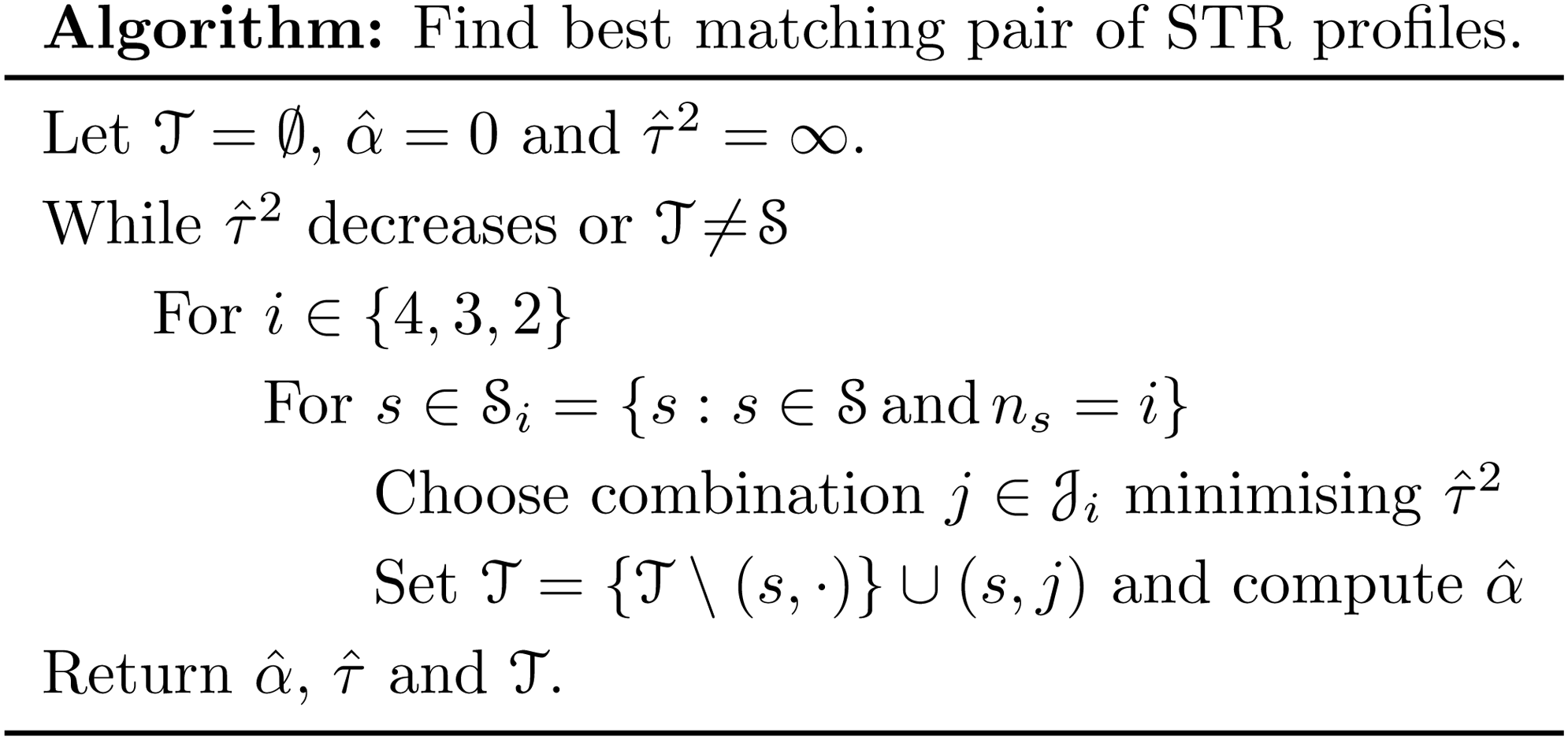
Greedy algorithm for finding a pair of profiles (locally) maximizing the likelihood of (1).
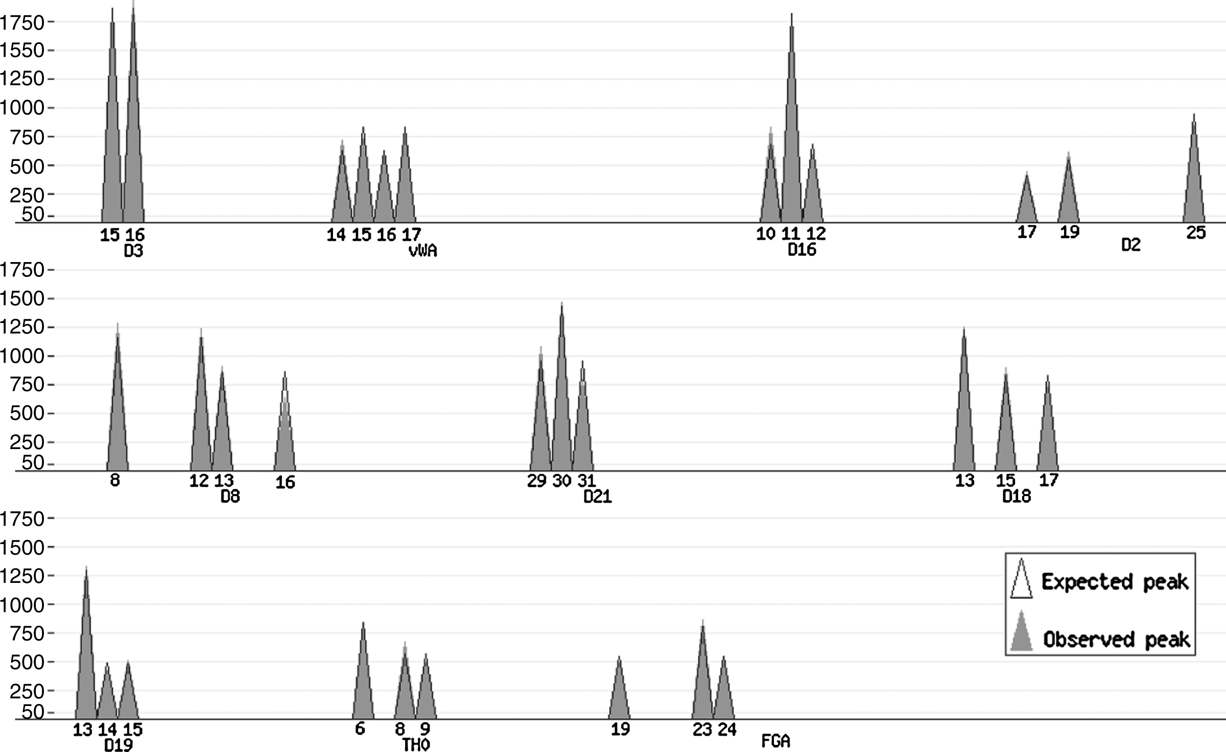
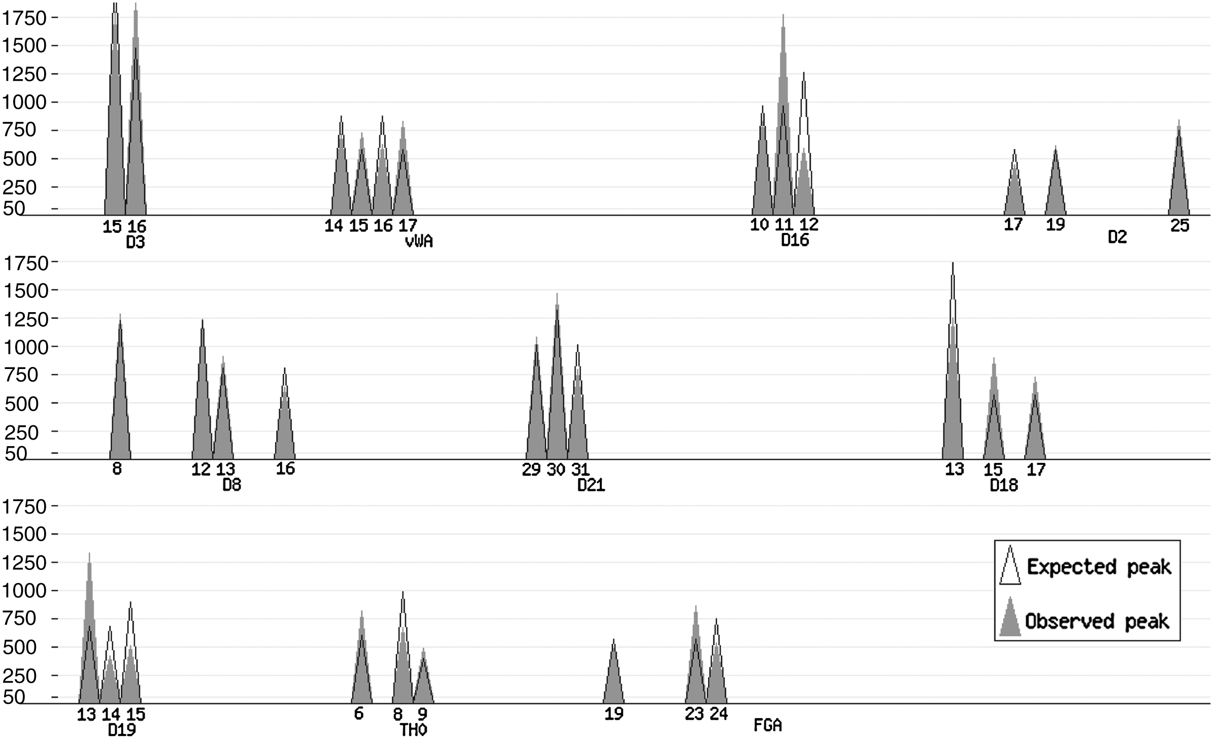
Plot produced by the on-line implementation of the algorithm (http://people.math.aau.dk/∼tvede/dna/—sample data file “Paper case”). The observed peaks, ▴, are based on data from Table 4, and the expected peaks, ▵, assuming a mixture of the best matching pair of STR profiles (Table 5). The observed and expected peaks coincide for nearly all peaks.
The Four STR Profiles Used in the Controlled Pairwise Two-Person Mixture Experiments
D3
vWA
D16
D2
D8
D21
D18
D19
TH0
FGA
A
14,18
17,19
12,14
20,24
10,13
30.2,32.2
13,13
12,13
8,9
20,22
B
15,16
14,16
10,12
17,25
13,16
30,30
13,13
14,15
6,9
19,23
C
15,16
15,17
11,11
19,25
8,12
29,31
15,17
13,13
6,8
23,24
D
16,19
15,17
10,12
23,25
13,13
28,30
12,16
13,15
6,7
20,23
3. Modeling Peak Areas of a Two-Person Mixture
For the search of a pair of best matching profiles to be feasible, we assume the peak areas of the various loci to be conditionally independent given the loci area sums, A+. Performing the inference conditioned on A+ satisfy the reasoning of Cox (1958) as A+ is an ancillary statistic for the mixture ratio, i.e. A+ is fixed for all values of the mixture ratio. Furthermore, we assume that the peak areas are multivariate normal distributed with conditional mean vector,
\documentclass{aastex}
\usepackage{amsbsy}
\usepackage{amsfonts}
\usepackage{amssymb}
\usepackage{bm}
\usepackage{mathrsfs}
\usepackage{pifont}
\usepackage{stmaryrd}
\usepackage{textcomp}
\usepackage{portland, xspace}
\usepackage{amsmath, amsxtra}
\pagestyle{empty}
\DeclareMathSizes {10} {9} {7} {6}
\begin{document}
$${\mathbb E} ( \textbf{\textit{A}}_s \mid A_{s , + } )$$
\end{document}, and covariance matrix,
\documentclass{aastex}
\usepackage{amsbsy}
\usepackage{amsfonts}
\usepackage{amssymb}
\usepackage{bm}
\usepackage{mathrsfs}
\usepackage{pifont}
\usepackage{stmaryrd}
\usepackage{textcomp}
\usepackage{portland, xspace}
\usepackage{amsmath, amsxtra}
\pagestyle{empty}
\DeclareMathSizes {10} {9} {7} {6}
\begin{document}
$${\mathbb C}{ \rm ov} ( \textbf{\textit{A}}_s \mid A_{s , + } )$$
\end{document}, defined as
\documentclass{aastex}
\usepackage{amsbsy}
\usepackage{amsfonts}
\usepackage{amssymb}
\usepackage{bm}
\usepackage{mathrsfs}
\usepackage{pifont}
\usepackage{stmaryrd}
\usepackage{textcomp}
\usepackage{portland, xspace}
\usepackage{amsmath, amsxtra}
\pagestyle{empty}
\DeclareMathSizes {10} {9} {7} {6}
\begin{document}
\begin{align*}
{\mathbb E} (\textbf {\textit {A}} _s \mid A_ {s , +}) & = [\alpha
\textbf {\textit {P}} _ {s , 1} + (1 - \alpha) \textbf {\textit
{P}} _ {s , 2}] \frac {A_ {s , +}} {2} \quad {\rm and} \\ {\mathbb
C} {\rm ov} (\textbf {\textit {A}} _s \mid A_ {s , +}) & = \tau^2
C_s {\rm diag} (\textbf {\textit {h}} _s) C_s^ {\top}, \tag {1}
\end{align*}
\end{document}
where α denotes the proportion with which person 1 contributes to the mixture, and
\documentclass{aastex}
\usepackage{amsbsy}
\usepackage{amsfonts}
\usepackage{amssymb}
\usepackage{bm}
\usepackage{mathrsfs}
\usepackage{pifont}
\usepackage{stmaryrd}
\usepackage{textcomp}
\usepackage{portland, xspace}
\usepackage{amsmath, amsxtra}
\pagestyle{empty}
\DeclareMathSizes {10} {9} {7} {6}
\begin{document}
$$C_s = I_{n_s} - n_s^{ - 1}\textbf{\textit{1}}_{n_s}\textbf{\textit{1}}_{n_s}^{ \top}$$
\end{document} with ns, 1 ≤ ns ≤ 4, being the number of observed peaks at locus s. Note that α is supposed to be common to all loci. The definition of the covariance matrix is close to the ordinary covariance when conditioning on the vector sum. However, as the variance of the peak area is assumed proportional to the mean, we use the diagonal matrix diag(hs), where hs is the associated peak heights on locus s, to obtain weighted observations that stabilise the variance. Furthermore, τ2 is a common variance parameter for all loci,
\documentclass{aastex}
\usepackage{amsbsy}
\usepackage{amsfonts}
\usepackage{amssymb}
\usepackage{bm}
\usepackage{mathrsfs}
\usepackage{pifont}
\usepackage{stmaryrd}
\usepackage{textcomp}
\usepackage{portland, xspace}
\usepackage{amsmath, amsxtra}
\pagestyle{empty}
\DeclareMathSizes {10} {9} {7} {6}
\begin{document}
$$s \in { \cal S}$$
\end{document}.
The Ps,k-vector is a vector of indicators taking values 0, 1 or 2 referring to the number of copies that person k has of each allele in the mixture on locus s. For example, if the two individuals contributing to the mixture have genotypes (10,12) and (14,14), respectively, we will have Ps,1 = (1, 1, 0)⊤ and Ps,2 = (0, 0, 2)⊤. Assuming no chromosomal anomalies, each individual carries two alleles at each locus which implies the sum of Ps,k to be 2 for all k.
The model presented here is different from, for example, the ones of Cowell et al. (2007a,b) and Curran (2008), who both take a Bayesian approach. The model of Cowell et al. (2007a) assumes the peak heights to be gamma-distributed to ensure proportionality of the mean and variance, whereas Cowell et al. (2007b) assumes normality of the peak heights with parameters chosen to ensure proportionality of mean and variance. As mentioned in Curran (2008), the model of Cowell et al. (2007a) makes a crude adjustment for a repeat number effect, which is no longer relevant. In Curran (2008), the peak heights are assumed multivariate normal, but here no attempt is done in order to ensure proportionality of the mean and variance. Furthermore, by conditioning on the peak area sums within each locus we acknowledge the strong inter-locus correlation. In addition to the methods based on statistical models, there are several methods that rely on heuristics and guidelines (Gill et al., 1998, 2006; Clayton et al., 1998; Perlin and Szabady, 2001; Bill et al., 2005; Wang et al., 2006). Cowell et al. (2007b) gives a nice review of most of these methods in their introductory section.
4. Finding Best Matching Pair of Profiles
In order to find the most likely pair of profiles matching the observed mixture under the assumptions made by the model, one can decrease the number of possibilities using the following arguments. Let the observed peak areas within each locus, s, be sorted such that
\documentclass{aastex}
\usepackage{amsbsy}
\usepackage{amsfonts}
\usepackage{amssymb}
\usepackage{bm}
\usepackage{mathrsfs}
\usepackage{pifont}
\usepackage{stmaryrd}
\usepackage{textcomp}
\usepackage{portland, xspace}
\usepackage{amsmath, amsxtra}
\pagestyle{empty}
\DeclareMathSizes {10} {9} {7} {6}
\begin{document}
$$A_{s , ( 1 ) } < \cdots < A_{s , ( n_s ) }$$
\end{document}, and assume that DNA1 < DNA2, where DNAk is the amount of DNA contributed by person k.
Then, for a locus with four observed peaks (ns = 4), the only likely pair of profiles given the model relate the alleles with peak areas (As,(1), As,(2)) and (As,(3), As,(4)) to person 1 and person 2, respectively. For loci with one observation (ns = 1), the two individuals need both to be homozygotic for the observed allele, while for two (ns = 2) or three observations (ns = 3), the possible profiles are listed in Table 3 (the notation
\documentclass{aastex}
\usepackage{amsbsy}
\usepackage{amsfonts}
\usepackage{amssymb}
\usepackage{bm}
\usepackage{mathrsfs}
\usepackage{pifont}
\usepackage{stmaryrd}
\usepackage{textcomp}
\usepackage{portland, xspace}
\usepackage{amsmath, amsxtra}
\pagestyle{empty}
\DeclareMathSizes {10} {9} {7} {6}
\begin{document}
$${ \cal J}_2$$
\end{document} and
\documentclass{aastex}
\usepackage{amsbsy}
\usepackage{amsfonts}
\usepackage{amssymb}
\usepackage{bm}
\usepackage{mathrsfs}
\usepackage{pifont}
\usepackage{stmaryrd}
\usepackage{textcomp}
\usepackage{portland, xspace}
\usepackage{amsmath, amsxtra}
\pagestyle{empty}
\DeclareMathSizes {10} {9} {7} {6}
\begin{document}
$${ \cal J}_3$$
\end{document} is used in Section 4.1).
Possible Profiles for Loci with Two and Three Observations
In Table 3, Ps,1 and Ps,2 refers to the profiles of person 1 and person 2 on the particular locus s, respectively, and the cell values to the number of alleles associated with the profiles. The reason for not considering the three and eight other combinations for loci with two and three observations (Table 1), respectively, is that, for any of these combinations, one of the four combinations listed in Table 3 will be more likely under the model assumptions, i.e., have a better fit to the observed data. For example, Ps,1 = (0, 2)⊤ and Ps,2 = (2,0)⊤ would be unlikely as we assumed person 1 to have the lowest contribution and the second area to be the larger.
Discarding the information from peak areas and only using combinatorics, the numbers of possible pairs of profiles for loci with two, three, and four observations are 7, 12, and 6, respectively. Thus, using the assumptions of the model, we decrease the number of profiles which needs to be examined in order to find the most likely profiles forming the observed mixture.
We assume the peak areas to be normally distributed with conditional means and covariances as specified in (1). Due to the conditional independence of the loci, the overall estimates of α and τ2 are found as sums over the loci. Let
\documentclass{aastex}
\usepackage{amsbsy}
\usepackage{amsfonts}
\usepackage{amssymb}
\usepackage{bm}
\usepackage{mathrsfs}
\usepackage{pifont}
\usepackage{stmaryrd}
\usepackage{textcomp}
\usepackage{portland, xspace}
\usepackage{amsmath, amsxtra}
\pagestyle{empty}
\DeclareMathSizes {10} {9} {7} {6}
\begin{document}
$$W_s = C_s{ \rm diag} ( \textbf{\textit{h}}_s ) C_s^{ \top}$$
\end{document}, then we can write the conditional distribution as
\documentclass{aastex}
\usepackage{amsbsy}
\usepackage{amsfonts}
\usepackage{amssymb}
\usepackage{bm}
\usepackage{mathrsfs}
\usepackage{pifont}
\usepackage{stmaryrd}
\usepackage{textcomp}
\usepackage{portland, xspace}
\usepackage{amsmath, amsxtra}
\pagestyle{empty}
\DeclareMathSizes {10} {9} {7} {6}
\begin{document}
$$\textbf{\textit{A}}_s \mid \textbf{\textit{A}}_{s , + } \sim {\cal N}_{n_s} ( \alpha \textbf{\textit{x}}_0^s - \textbf{\textit{x}}_1^s , \tau^2W_s )$$
\end{document}, where
\documentclass{aastex}
\usepackage{amsbsy}
\usepackage{amsfonts}
\usepackage{amssymb}
\usepackage{bm}
\usepackage{mathrsfs}
\usepackage{pifont}
\usepackage{stmaryrd}
\usepackage{textcomp}
\usepackage{portland, xspace}
\usepackage{amsmath, amsxtra}
\pagestyle{empty}
\DeclareMathSizes {10} {9} {7} {6}
\begin{document}
$$\textbf{\textit{x}}_0^s = ( \textbf{\textit{P}}_{s , 1} - \textbf{\textit{P}}_{s , 2} ) A_{s , + } / 2$$
\end{document} and
\documentclass{aastex}
\usepackage{amsbsy}
\usepackage{amsfonts}
\usepackage{amssymb}
\usepackage{bm}
\usepackage{mathrsfs}
\usepackage{pifont}
\usepackage{stmaryrd}
\usepackage{textcomp}
\usepackage{portland, xspace}
\usepackage{amsmath, amsxtra}
\pagestyle{empty}
\DeclareMathSizes {10} {9} {7} {6}
\begin{document}
$$\textbf{\textit{x}}_1^s = \textbf{\textit{P}}_{s , 2}A_{s , + } / 2$$
\end{document} are the terms of the mean, linear and constant in α, respectively. Solving the likelihood equation with respect to α and τ2 yield the unbiased estimators
\documentclass{aastex}
\usepackage{amsbsy}
\usepackage{amsfonts}
\usepackage{amssymb}
\usepackage{bm}
\usepackage{mathrsfs}
\usepackage{pifont}
\usepackage{stmaryrd}
\usepackage{textcomp}
\usepackage{portland, xspace}
\usepackage{amsmath, amsxtra}
\pagestyle{empty}
\DeclareMathSizes {10} {9} {7} {6}
\begin{document}
\begin{align*}
\hat {\alpha} & = \frac {\sum_ {s \in {\cal S}} \textbf {\textit {x}} { _0^s} ^ {\top} W_s^ {-} (\textbf {\textit {A}} _s - x_1^s )} {\sum_ {s \in {\cal S}} \textbf {\textit {x}} {_0^s} ^ {\top} W_s^ {-} x_0^s} \quad {\rm and} \\ \hat {\tau} ^2 & = N^ {- 1} \sum_ {s \in {\cal S}} (\textbf {\textit {A}} _s - \hat {\alpha} \textbf {\textit {x}} _0^s - \textbf {\textit {x} } _1^s) ^ {\top} W_s^ {-} (\textbf {\textit {A}} _s - \hat {\alpha} \textbf {\textit {x}} _0^s - \textbf {\textit {x}} _1^s ), \tag {2}
\end{align*}
\end{document}
where
\documentclass{aastex}
\usepackage{amsbsy}
\usepackage{amsfonts}
\usepackage{amssymb}
\usepackage{bm}
\usepackage{mathrsfs}
\usepackage{pifont}
\usepackage{stmaryrd}
\usepackage{textcomp}
\usepackage{portland, xspace}
\usepackage{amsmath, amsxtra}
\pagestyle{empty}
\DeclareMathSizes {10} {9} {7} {6}
\begin{document}
$$N = n_{ + } - S - 1 = \sum \nolimits_{s \in { \cal S}} ( n_s - 1 ) - 1$$
\end{document} and
\documentclass{aastex}
\usepackage{amsbsy}
\usepackage{amsfonts}
\usepackage{amssymb}
\usepackage{bm}
\usepackage{mathrsfs}
\usepackage{pifont}
\usepackage{stmaryrd}
\usepackage{textcomp}
\usepackage{portland, xspace}
\usepackage{amsmath, amsxtra}
\pagestyle{empty}
\DeclareMathSizes {10} {9} {7} {6}
\begin{document}
$$W_s^{ - }$$
\end{document} is the generalized inverse of Ws. We have to use the generalized inverse of Ws as Ws has the rank ns − 1. An approximation to this model assumes that the precision matrix,
\documentclass{aastex}
\usepackage{amsbsy}
\usepackage{amsfonts}
\usepackage{amssymb}
\usepackage{bm}
\usepackage{mathrsfs}
\usepackage{pifont}
\usepackage{stmaryrd}
\usepackage{textcomp}
\usepackage{portland, xspace}
\usepackage{amsmath, amsxtra}
\pagestyle{empty}
\DeclareMathSizes {10} {9} {7} {6}
\begin{document}
$$\tau^{ - 2}W_s^{ - 1}$$
\end{document}, is given by
\documentclass{aastex}
\usepackage{amsbsy}
\usepackage{amsfonts}
\usepackage{amssymb}
\usepackage{bm}
\usepackage{mathrsfs}
\usepackage{pifont}
\usepackage{stmaryrd}
\usepackage{textcomp}
\usepackage{portland, xspace}
\usepackage{amsmath, amsxtra}
\pagestyle{empty}
\DeclareMathSizes {10} {9} {7} {6}
\begin{document}
$$\tau^{ - 2}C_s{ \rm diag} ( \textbf{\textit{h}}_s ) ^{ - 1}C_s^{ \top}$$
\end{document}. Hence, we have a closed form expression for the inverse covariance matrix yielding simple expressions for the estimators of α and τ2,
\documentclass{aastex}
\usepackage{amsbsy}
\usepackage{amsfonts}
\usepackage{amssymb}
\usepackage{bm}
\usepackage{mathrsfs}
\usepackage{pifont}
\usepackage{stmaryrd}
\usepackage{textcomp}
\usepackage{portland, xspace}
\usepackage{amsmath, amsxtra}
\pagestyle{empty}
\DeclareMathSizes {10} {9} {7} {6}
\begin{document}
\begin{align*}
\tilde { \alpha } & = \frac { \sum_ { s \in { \cal S } } \sum_ { i
= 1 } ^ { n_s } x_ { 0 , i } ^s ( A_ { s , i } - x_ { 1 , i } ^s )
h^ { - 1 } _ { s , i } } { \sum_ { s \in { \cal S } } \sum_ { i =
1 } ^ { n_s } { x_ { 0 , i } ^s } ^2h^ { - 1 } _ { s , i } } \quad
{ \rm and } \\ \tilde { \tau } ^2 & = N^ { - 1 } \sum_ { s \in {
\cal S } } \sum_ { i = 1 } ^ { n_s } ( A_ { s , i } - \tilde {
\alpha } x_ { 0 , i } ^s - x_ { 1 , i } ^s ) ^2h^ { - 1 } _ { s ,
i } ,
\end{align*}
\end{document}
where
\documentclass{aastex}
\usepackage{amsbsy}
\usepackage{amsfonts}
\usepackage{amssymb}
\usepackage{bm}
\usepackage{mathrsfs}
\usepackage{pifont}
\usepackage{stmaryrd}
\usepackage{textcomp}
\usepackage{portland, xspace}
\usepackage{amsmath, amsxtra}
\pagestyle{empty}
\DeclareMathSizes {10} {9} {7} {6}
\begin{document}
$$A_{s , i , } h_{s , i , }x_{0 , i}^s$$
\end{document} and
\documentclass{aastex}
\usepackage{amsbsy}
\usepackage{amsfonts}
\usepackage{amssymb}
\usepackage{bm}
\usepackage{mathrsfs}
\usepackage{pifont}
\usepackage{stmaryrd}
\usepackage{textcomp}
\usepackage{portland, xspace}
\usepackage{amsmath, amsxtra}
\pagestyle{empty}
\DeclareMathSizes {10} {9} {7} {6}
\begin{document}
$$x_{1 , i}^s$$
\end{document} are the i'th components of the respective bold faced vectors. We denote the unbiased maximum likelihood estimates for the two models as (
\documentclass{aastex}
\usepackage{amsbsy}
\usepackage{amsfonts}
\usepackage{amssymb}
\usepackage{bm}
\usepackage{mathrsfs}
\usepackage{pifont}
\usepackage{stmaryrd}
\usepackage{textcomp}
\usepackage{portland, xspace}
\usepackage{amsmath, amsxtra}
\pagestyle{empty}
\DeclareMathSizes {10} {9} {7} {6}
\begin{document}
$$\hat{ \alpha} , \hat{ \tau}$$
\end{document}) and (
\documentclass{aastex}
\usepackage{amsbsy}
\usepackage{amsfonts}
\usepackage{amssymb}
\usepackage{bm}
\usepackage{mathrsfs}
\usepackage{pifont}
\usepackage{stmaryrd}
\usepackage{textcomp}
\usepackage{portland, xspace}
\usepackage{amsmath, amsxtra}
\pagestyle{empty}
\DeclareMathSizes {10} {9} {7} {6}
\begin{document}
$$\tilde{ \alpha} , \tilde{ \tau}$$
\end{document}), respectively. The latter version is what is implemented in an on-line tool as discussed in Section 4.2.
In addition to the estimate of α, we are also interested in determining a confidence interval for α. The conditional variance of
\documentclass{aastex}
\usepackage{amsbsy}
\usepackage{amsfonts}
\usepackage{amssymb}
\usepackage{bm}
\usepackage{mathrsfs}
\usepackage{pifont}
\usepackage{stmaryrd}
\usepackage{textcomp}
\usepackage{portland, xspace}
\usepackage{amsmath, amsxtra}
\pagestyle{empty}
\DeclareMathSizes {10} {9} {7} {6}
\begin{document}
$$\hat{ \alpha}$$
\end{document} given A+ is found using the covariance operator on both sides of (2),
\documentclass{aastex}
\usepackage{amsbsy}
\usepackage{amsfonts}
\usepackage{amssymb}
\usepackage{bm}
\usepackage{mathrsfs}
\usepackage{pifont}
\usepackage{stmaryrd}
\usepackage{textcomp}
\usepackage{portland, xspace}
\usepackage{amsmath, amsxtra}
\pagestyle{empty}
\DeclareMathSizes {10} {9} {7} {6}
\begin{document}
\begin{align*}
{\mathbb V} {\rm ar} (\hat {\alpha} \mid \textbf {\textit {A}} _ {+} ) & = \frac {{\mathbb C} {\rm ov} \left(\sum_ {s \in {\cal S}} \textbf {\textit {x}} _0^s { } ^ {\top} W_s^ - (\textbf {\textit {A}} _s - \textbf {\textit {x}} _1^s) \big| \textbf {\textit {A}} _ {+} \right)} {\left(\sum_ {s \in { \cal S}} \textbf {\textit {x}} _0^s { } ^ {\top} W_s^ - \textbf {\textit {x } } _0^s \right)^2} \\ & = \frac { \sum_ {s \in {\cal S}} \textbf {\textit {x} } _0^s { } ^ {\top} W_s^ - { \mathbb C } { \rm ov } ( \textbf { \textit { A } } _s \mid \textbf { \textit { A } } _ { + } ) W_s^ - \textbf { \textit { x } } _0^s } { ( \sum_ { s \in { \cal S } } \textbf { \textit { x } } _0^s { } ^ { \top } W_s^ - \textbf { \textit { x } } _0^s ) ^2 } \\ & = \tau^2 \left(\sum_ { s \in { s } } \textbf { \textit { x } } _0^s { } ^ { \top } W_s^ - \textbf { \textit { x } } _0^s \right)^ { - 1 } , \tag {3}
\end{align*}
\end{document}
where we, from the first to second equality, used the conditional independence of As and At given A+, and second to third properties of the covariance together with the expression of
\documentclass{aastex}
\usepackage{amsbsy}
\usepackage{amsfonts}
\usepackage{amssymb}
\usepackage{bm}
\usepackage{mathrsfs}
\usepackage{pifont}
\usepackage{stmaryrd}
\usepackage{textcomp}
\usepackage{portland, xspace}
\usepackage{amsmath, amsxtra}
\pagestyle{empty}
\DeclareMathSizes {10} {9} {7} {6}
\begin{document}
$${\mathbb C}{ \rm ov} ( \textbf{\textit{A}}_s \mid \textbf{\textit{A}}_{ + } )$$
\end{document} in (1). The confidence interval of α given A+ is then given by
\documentclass{aastex}
\usepackage{amsbsy}
\usepackage{amsfonts}
\usepackage{amssymb}
\usepackage{bm}
\usepackage{mathrsfs}
\usepackage{pifont}
\usepackage{stmaryrd}
\usepackage{textcomp}
\usepackage{portland, xspace}
\usepackage{amsmath, amsxtra}
\pagestyle{empty}
\DeclareMathSizes {10} {9} {7} {6}
\begin{document}
\begin{align*}
{ \bf CI } _ { \beta } ( { \alpha } ) = \hat { \alpha } \pm t_ { 1
- \beta / 2 , N } \frac { \hat { \tau } } { \sqrt { \sum_ { s \in
{ \cal S } } \textbf { \textit { x } } _0^s { } ^ { \top } W_s^ -
\textbf { \textit { x } } _0^s } } ,
\end{align*}
\end{document}
where t1 − β/2,N is the critical value on significance level β for a t-distribution with N = n+ − S − 1 degrees of freedom. A similar confidence interval using the (
\documentclass{aastex}
\usepackage{amsbsy}
\usepackage{amsfonts}
\usepackage{amssymb}
\usepackage{bm}
\usepackage{mathrsfs}
\usepackage{pifont}
\usepackage{stmaryrd}
\usepackage{textcomp}
\usepackage{portland, xspace}
\usepackage{amsmath, amsxtra}
\pagestyle{empty}
\DeclareMathSizes {10} {9} {7} {6}
\begin{document}
$$\tilde{ \alpha} , \tilde{ \tau}$$
\end{document})-estimates is obtained by inserting the (
\documentclass{aastex}
\usepackage{amsbsy}
\usepackage{amsfonts}
\usepackage{amssymb}
\usepackage{bm}
\usepackage{mathrsfs}
\usepackage{pifont}
\usepackage{stmaryrd}
\usepackage{textcomp}
\usepackage{portland, xspace}
\usepackage{amsmath, amsxtra}
\pagestyle{empty}
\DeclareMathSizes {10} {9} {7} {6}
\begin{document}
$$\tilde{ \alpha} , \tilde{ \tau}$$
\end{document})-estimates instead of (
\documentclass{aastex}
\usepackage{amsbsy}
\usepackage{amsfonts}
\usepackage{amssymb}
\usepackage{bm}
\usepackage{mathrsfs}
\usepackage{pifont}
\usepackage{stmaryrd}
\usepackage{textcomp}
\usepackage{portland, xspace}
\usepackage{amsmath, amsxtra}
\pagestyle{empty}
\DeclareMathSizes {10} {9} {7} {6}
\begin{document}
$$\hat{ \alpha} , \hat{ \tau}$$
\end{document}) and replacing W− with W−1. From the expression of CIβ(α), it is obvious that a small τ-estimate decreases the width of the confidence interval and thus increases the trust in the estimated mixture proportion.
4.1. Greedy algorithm
This model was used in an algorithm for finding the most likely pair of profiles contributing to an observed mixture where the STR profiles of both individuals were assumed unknown. First, define the set
\documentclass{aastex}
\usepackage{amsbsy}
\usepackage{amsfonts}
\usepackage{amssymb}
\usepackage{bm}
\usepackage{mathrsfs}
\usepackage{pifont}
\usepackage{stmaryrd}
\usepackage{textcomp}
\usepackage{portland, xspace}
\usepackage{amsmath, amsxtra}
\pagestyle{empty}
\DeclareMathSizes {10} {9} {7} {6}
\begin{document}
$${ \cal J} = \{ { \cal J}_1 , \ldots , { \cal J}_4 \} $$
\end{document}, where
\documentclass{aastex}
\usepackage{amsbsy}
\usepackage{amsfonts}
\usepackage{amssymb}
\usepackage{bm}
\usepackage{mathrsfs}
\usepackage{pifont}
\usepackage{stmaryrd}
\usepackage{textcomp}
\usepackage{portland, xspace}
\usepackage{amsmath, amsxtra}
\pagestyle{empty}
\DeclareMathSizes {10} {9} {7} {6}
\begin{document}
$${ \cal J}_i$$
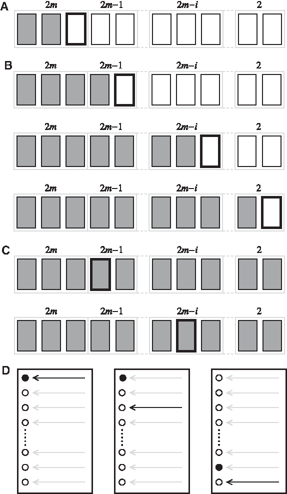
\end{document} is the set of plausible profiles for loci with ns = i. These sets were defined in Section 4 (Table 3). The pseudo code for a greedy algorithm finding a pair of profiles (locally) maximising the likelihood of the model specified by (1) is given in Figure 1. A greedy algorithm is any algorithm that solves a problem by making the locally optimum choice at each stage with the hope of finding the global optimum. A graphical representation of the algorithm is given in Figure 7 below for a general number of contributors, m. The algorithm works with both (
\documentclass{aastex}
\usepackage{amsbsy}
\usepackage{amsfonts}
\usepackage{amssymb}
\usepackage{bm}
\usepackage{mathrsfs}
\usepackage{pifont}
\usepackage{stmaryrd}
\usepackage{textcomp}
\usepackage{portland, xspace}
\usepackage{amsmath, amsxtra}
\pagestyle{empty}
\DeclareMathSizes {10} {9} {7} {6}
\begin{document}
$$\hat{ \alpha} , \hat{ \tau}$$
\end{document}) or (
\documentclass{aastex}
\usepackage{amsbsy}
\usepackage{amsfonts}
\usepackage{amssymb}
\usepackage{bm}
\usepackage{mathrsfs}
\usepackage{pifont}
\usepackage{stmaryrd}
\usepackage{textcomp}
\usepackage{portland, xspace}
\usepackage{amsmath, amsxtra}
\pagestyle{empty}
\DeclareMathSizes {10} {9} {7} {6}
\begin{document}
$$\tilde{ \alpha} , \tilde{ \tau}$$
\end{document}) as estimates of (α, τ).
The greedy algorithm initiates by estimating α based on a locus s with four present alleles. The loci of
\documentclass{aastex}
\usepackage{amsbsy}
\usepackage{amsfonts}
\usepackage{amssymb}
\usepackage{bm}
\usepackage{mathrsfs}
\usepackage{pifont}
\usepackage{stmaryrd}
\usepackage{textcomp}
\usepackage{portland, xspace}
\usepackage{amsmath, amsxtra}
\pagestyle{empty}
\DeclareMathSizes {10} {9} {7} {6}
\begin{document}
$${ \cal S}_4$$
\end{document} contain full information on the mixture ratio, α, and are thus used for assessing this quantity. In succession, the loci with three and two (
\documentclass{aastex}
\usepackage{amsbsy}
\usepackage{amsfonts}
\usepackage{amssymb}
\usepackage{bm}
\usepackage{mathrsfs}
\usepackage{pifont}
\usepackage{stmaryrd}
\usepackage{textcomp}
\usepackage{portland, xspace}
\usepackage{amsmath, amsxtra}
\pagestyle{empty}
\DeclareMathSizes {10} {9} {7} {6}
\begin{document}
$${ \cal S}_3$$
\end{document} and
\documentclass{aastex}
\usepackage{amsbsy}
\usepackage{amsfonts}
\usepackage{amssymb}
\usepackage{bm}
\usepackage{mathrsfs}
\usepackage{pifont}
\usepackage{stmaryrd}
\usepackage{textcomp}
\usepackage{portland, xspace}
\usepackage{amsmath, amsxtra}
\pagestyle{empty}
\DeclareMathSizes {10} {9} {7} {6}
\begin{document}
$${ \cal S}_2$$
\end{document}, respectively) observations are analyzed and the combination with the smallest contribution to τ and best concordance to the previously determined mixture proportion is chosen. The set
\documentclass{aastex}
\usepackage{amsbsy}
\usepackage{amsfonts}
\usepackage{amssymb}
\usepackage{bm}
\usepackage{mathrsfs}
\usepackage{pifont}
\usepackage{stmaryrd}
\usepackage{textcomp}
\usepackage{portland, xspace}
\usepackage{amsmath, amsxtra}
\pagestyle{empty}
\DeclareMathSizes {10} {9} {7} {6}
\begin{document}
$${ \cal T}$$
\end{document} contains a list of the optimal combinations on previously visited loci and is updated after each iteration. On termination, the greedy algorithm returns the best matching pair of profiles together with the estimates of α and τ. The algorithm is designed to perform calculations and decisions similar to those of a forensic geneticist when analyzing a two-person mixture.
The optimization problem is complicated since the inputs of the function that we are interested in minimizing depend on each other,
\documentclass{aastex}
\usepackage{amsbsy}
\usepackage{amsfonts}
\usepackage{amssymb}
\usepackage{bm}
\usepackage{mathrsfs}
\usepackage{pifont}
\usepackage{stmaryrd}
\usepackage{textcomp}
\usepackage{portland, xspace}
\usepackage{amsmath, amsxtra}
\pagestyle{empty}
\DeclareMathSizes {10} {9} {7} {6}
\begin{document}
$$f ( \alpha , ( \textbf{\textit{P}}_{s , 1} , \textbf{\textit{P}}_{s , 2} ) _{s \in { \cal S}} ) = \sum \nolimits_{s \in { \cal S}}D_s$$
\end{document}, where
\documentclass{aastex}
\usepackage{amsbsy}
\usepackage{amsfonts}
\usepackage{amssymb}
\usepackage{bm}
\usepackage{mathrsfs}
\usepackage{pifont}
\usepackage{stmaryrd}
\usepackage{textcomp}
\usepackage{portland, xspace}
\usepackage{amsmath, amsxtra}
\pagestyle{empty}
\DeclareMathSizes {10} {9} {7} {6}
\begin{document}
$$D_s = ( \textbf{\textit{A}}_s - \alpha \textbf{\textit{x}}_0^s - \textbf{\textit{x}}_1^s ) ^{ \top}W_s^{ - } ( \textbf{\textit{A}}_s - \alpha \textbf{\textit{x}}_0^s - \textbf{\textit{x}}_1^s )$$
\end{document}. Here, f denotes the object function and
\documentclass{aastex}
\usepackage{amsbsy}
\usepackage{amsfonts}
\usepackage{amssymb}
\usepackage{bm}
\usepackage{mathrsfs}
\usepackage{pifont}
\usepackage{stmaryrd}
\usepackage{textcomp}
\usepackage{portland, xspace}
\usepackage{amsmath, amsxtra}
\pagestyle{empty}
\DeclareMathSizes {10} {9} {7} {6}
\begin{document}
$$( \textbf{\textit{P}}_{s , 1 , } \textbf{\textit{P}}_{s , 2} ) _{s \in { \cal S}}$$
\end{document} the set of possible combinations for all loci,
\documentclass{aastex}
\usepackage{amsbsy}
\usepackage{amsfonts}
\usepackage{amssymb}
\usepackage{bm}
\usepackage{mathrsfs}
\usepackage{pifont}
\usepackage{stmaryrd}
\usepackage{textcomp}
\usepackage{portland, xspace}
\usepackage{amsmath, amsxtra}
\pagestyle{empty}
\DeclareMathSizes {10} {9} {7} {6}
\begin{document}
$$s \in { \cal S}$$
\end{document}. It is easy to see that, for a fixed α, we can minimize Ds for each locus s by choosing the combination yielding the smallest square distance. Similarly, fixing the combinations for all loci, α is estimated using (2). However, from the construction of the greedy algorithm, the algorithm chooses the combination that minimizes τ2 for locus s given α and the configurations on loci previously visited loci,
\documentclass{aastex}
\usepackage{amsbsy}
\usepackage{amsfonts}
\usepackage{amssymb}
\usepackage{bm}
\usepackage{mathrsfs}
\usepackage{pifont}
\usepackage{stmaryrd}
\usepackage{textcomp}
\usepackage{portland, xspace}
\usepackage{amsmath, amsxtra}
\pagestyle{empty}
\DeclareMathSizes {10} {9} {7} {6}
\begin{document}
$$t \in \{ { \cal T} \setminus s \} $$
\end{document}. This ensures locally optimal solutions, and for most practical purposes, the algorithm returns a global maximum. One should note that, when the algorithm recovers the best matching pair of profiles, we still need to consider all profiles close to these profiles consistent with the evidence for likelihood ratio evaluation (for further details, see Section 5).
4.2. On-line implementation
The greedy algorithm of Figure 1 together with the methods for evaluating the goodness of fit for a given pair of profiles are implemented in an online application. The on-line implementation applies the (
\documentclass{aastex}
\usepackage{amsbsy}
\usepackage{amsfonts}
\usepackage{amssymb}
\usepackage{bm}
\usepackage{mathrsfs}
\usepackage{pifont}
\usepackage{stmaryrd}
\usepackage{textcomp}
\usepackage{portland, xspace}
\usepackage{amsmath, amsxtra}
\pagestyle{empty}
\DeclareMathSizes {10} {9} {7} {6}
\begin{document}
$$\tilde{ \alpha} , \tilde{ \tau}$$
\end{document})-estimates when finding the best matching pair of profiles. The two-person (and three-person) mixture separator is available online at the first author's website (http://people.math.aau.dk/∼tvede/dna/). The script can plot the expected and observed peak areas for visual inspection of the fit (Fig. 2).
The script allows for user uploads of csv-files containing information about loci, alleles, peak heights, and peak areas. The loci implemented are those contained in the SGM Plus and Identifiler kits (Applied Biosystems) excluding amelogenin.
Apart from finding the best matching pair of unknown profiles, the user can specify a suspect profile, and the script finds the best matching unknown profile for two-person mixtures.
4.2.1. Example of a two-person mixture separation
We demonstrate the algorithm and implementation on data from a controlled experiment conducted at the Section of Forensic Genetics, Department of Forensic Medicine, Faculty of Health Sciences, University of Copenhagen, Denmark. The data are presented in Table 4 together with information on the true profiles of the mixture (denoted by ∘ and •).
Data Used in Demonstrating the Algorithm
Locus
Allele
Height
Area
Locus
Allele
Height
Area
D3
15
∘ •
1802
15410
D21
29
•
1073
9454
D3
16
∘ •
1939
16282
D21
30
∘
1469
12828
vWA
14
∘
712
6128
D21
31
•
798
6992
vWA
15
•
725
6620
D18
13
∘
1247
12302
vWA
16
∘
626
5637
D18
15
•
899
9104
vWA
17
•
830
7362
D18
17
•
726
7549
D16
10
∘
824
7910
D19
13
•
1332
10534
D16
11
•
1772
17231
D19
14
∘
416
3478
D16
12
∘
586
6101
D19
15
∘
504
3968
D2
17
∘
434
4558
TH0
6
∘ •
820
6739
D2
19
•
612
6563
TH0
8
•
668
5573
D2
25
∘ •
843
9257
TH0
9
∘
486
4004
D8
8
•
1284
10782
FGA
19
∘
490
4415
D8
12
•
1232
10359
FGA
23
∘•
865
7968
D8
13
∘
903
7891
FGA
24
•
527
5036
D8
16
∘
638
5291
The ∘ and • represents profile 1 and 2, respectively.
The algorithm found that the two profiles of Table 5 are the best matching pair of profiles. The profiles are consistent with the true profiles of the mixture except for loci TH0 and FGA. In Figure 2, we have plotted the data from Table 4 (solid cones, ▴) together with the best matching pair of profiles as listed in Table 5.
Best Matching Pair of Profiles for the Data inTable 4
Locus
D3
vWA
D16
D2
D8
D21
D18
D19
TH0
FGA
Minor
15,16
14,16
10,12
17,25
13,16
30,30
13,13
14,15
6,6
23,23
Major
15,16
15,17
11,11
19,25
8,12
29,31
15,17
13,13
8,9
19,24
This pair of profiles is pictured in Figure 2 as the expected peaks.
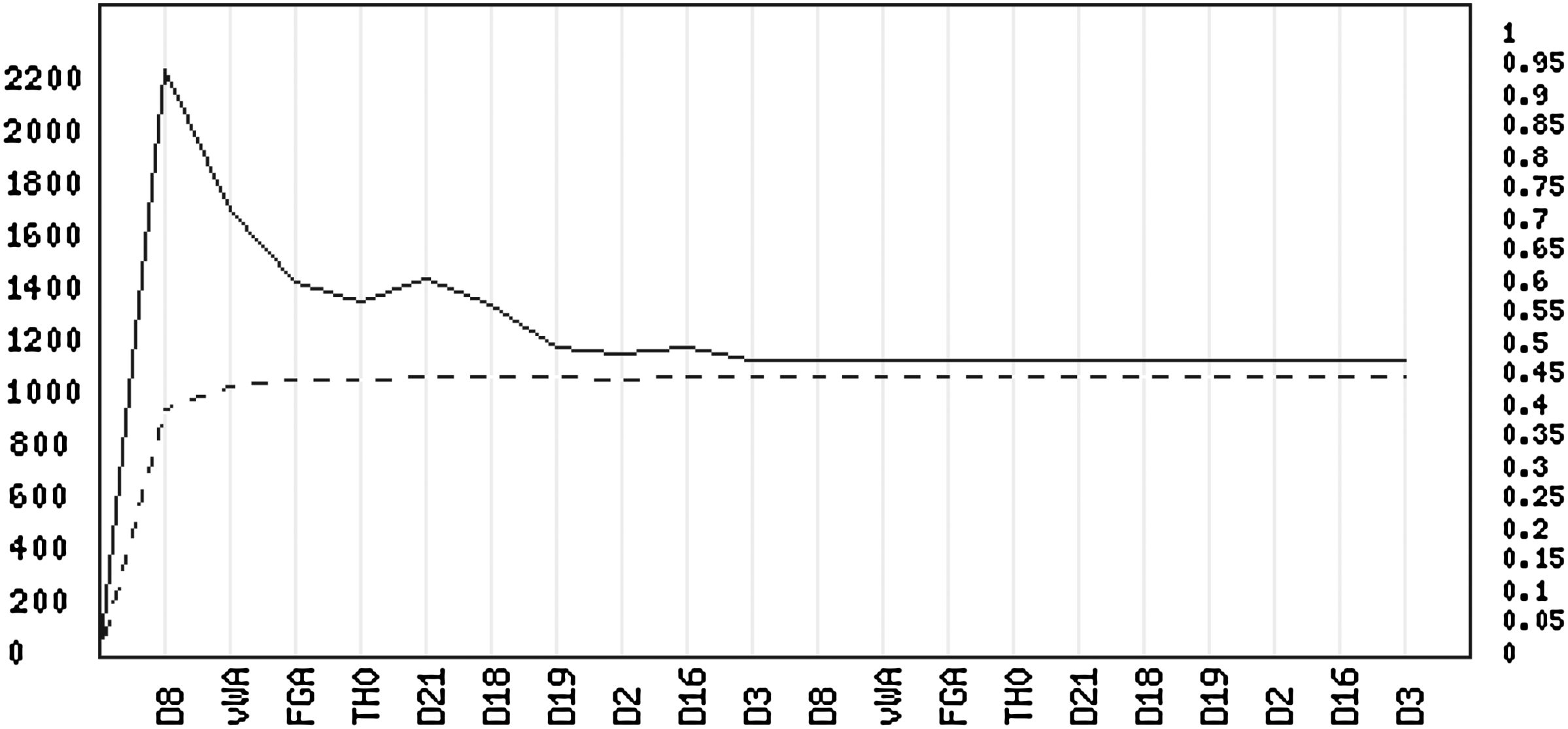
In Figure 3, the traces of the parameter estimates of α (dashed) and τ2 (solid) are plotted for each successive iteration, with the final parameter estimates being
\documentclass{aastex}
\usepackage{amsbsy}
\usepackage{amsfonts}
\usepackage{amssymb}
\usepackage{bm}
\usepackage{mathrsfs}
\usepackage{pifont}
\usepackage{stmaryrd}
\usepackage{textcomp}
\usepackage{portland, xspace}
\usepackage{amsmath, amsxtra}
\pagestyle{empty}
\DeclareMathSizes {10} {9} {7} {6}
\begin{document}
$$\tilde{ \alpha} = 0.43$$
\end{document} (95%-CI: [0.40; 0.45]) and
\documentclass{aastex}
\usepackage{amsbsy}
\usepackage{amsfonts}
\usepackage{amssymb}
\usepackage{bm}
\usepackage{mathrsfs}
\usepackage{pifont}
\usepackage{stmaryrd}
\usepackage{textcomp}
\usepackage{portland, xspace}
\usepackage{amsmath, amsxtra}
\pagestyle{empty}
\DeclareMathSizes {10} {9} {7} {6}
\begin{document}
$$\tilde{ \tau}^2 = 1134.04$$
\end{document}. Evaluating the mixture of the true profiles (marked by ∘ and • in Table 4), the α estimate is almost unchanged (
\documentclass{aastex}
\usepackage{amsbsy}
\usepackage{amsfonts}
\usepackage{amssymb}
\usepackage{bm}
\usepackage{mathrsfs}
\usepackage{pifont}
\usepackage{stmaryrd}
\usepackage{textcomp}
\usepackage{portland, xspace}
\usepackage{amsmath, amsxtra}
\pagestyle{empty}
\DeclareMathSizes {10} {9} {7} {6}
\begin{document}
$$\tilde{ \alpha} = 0.42$$
\end{document}), but with an increase in
\documentclass{aastex}
\usepackage{amsbsy}
\usepackage{amsfonts}
\usepackage{amssymb}
\usepackage{bm}
\usepackage{mathrsfs}
\usepackage{pifont}
\usepackage{stmaryrd}
\usepackage{textcomp}
\usepackage{portland, xspace}
\usepackage{amsmath, amsxtra}
\pagestyle{empty}
\DeclareMathSizes {10} {9} {7} {6}
\begin{document}
$$\tilde{ \tau}^2$$
\end{document} to 1266.34 indicating a slightly worse fit.
Trace of the parameter estimates of α (dashed/right ordinate labels) and τ2 (solid/left ordinate labels). The plot is produced by the on-line tool available at http://people.math.aau.dk/∼tvede/dna/.
The fact that a combination different from the true one has a better fit indicates that there are multiple explanations of the trace since it is a 1:1-mixture (α close to 0.5). However, the difference in τ2-estimates for the two combinations will only have a minor influence in the evaluation of the evidence.
4.3. Dropping non-fitting loci
In some cases, the stain may be contaminated, and it may be subject to drop-in or drop-out. Drop-ins are allelic peaks present in the DNA profile not belonging to the true profiles. Drop-ins may occur at random (contamination) or by more systematic mechanisms such as stuttering or pull-up effects. Stutters are caused by artefacts in the polymerase chain reaction resulting in an increase of peak intensities typically in the allelic position before the true peaks. Pull-up effects are manifested as an increase of true peaks caused by overlap of the spectra of the light emitted from the various fluorochromes, which are detected by a CCD camera in the data generating process (Butler, 2005). Drop-outs are allelic peaks of the true profiles that are absent in the DNA profile due to, for example, low amount of DNA or degradation of the DNA. In such cases, the observed peak heights and peak areas no longer originates solely from a two-person mixture. Hence, the proportionalities of Section 1 need no longer to be satisfied, and the mean structure of (1) may not explain the observed peak heights and peak areas in all loci.
We use an F-test approach to evaluate whether any of the included loci
\documentclass{aastex}
\usepackage{amsbsy}
\usepackage{amsfonts}
\usepackage{amssymb}
\usepackage{bm}
\usepackage{mathrsfs}
\usepackage{pifont}
\usepackage{stmaryrd}
\usepackage{textcomp}
\usepackage{portland, xspace}
\usepackage{amsmath, amsxtra}
\pagestyle{empty}
\DeclareMathSizes {10} {9} {7} {6}
\begin{document}
$$s \in { \cal S}$$
\end{document} has significant unexpected balances due to, for example, stutters, degradation, or contamination. The purpose is to return a list of loci in which the hypothesis of a two-person mixture can be supported.
For each locus, the contribution to τ2 is computed by Ds, which we assume to follow a
\documentclass{aastex}
\usepackage{amsbsy}
\usepackage{amsfonts}
\usepackage{amssymb}
\usepackage{bm}
\usepackage{mathrsfs}
\usepackage{pifont}
\usepackage{stmaryrd}
\usepackage{textcomp}
\usepackage{portland, xspace}
\usepackage{amsmath, amsxtra}
\pagestyle{empty}
\DeclareMathSizes {10} {9} {7} {6}
\begin{document}
$$\chi_{n_s - 1}^2$$
\end{document}-distribution. Hence, to test whether any locus contributes significantly to the overall variance, τ2, we evaluate for each locus
\documentclass{aastex}
\usepackage{amsbsy}
\usepackage{amsfonts}
\usepackage{amssymb}
\usepackage{bm}
\usepackage{mathrsfs}
\usepackage{pifont}
\usepackage{stmaryrd}
\usepackage{textcomp}
\usepackage{portland, xspace}
\usepackage{amsmath, amsxtra}
\pagestyle{empty}
\DeclareMathSizes {10} {9} {7} {6}
\begin{document}
$$s \in { \cal S}$$
\end{document} the ratio
\documentclass{aastex}
\usepackage{amsbsy}
\usepackage{amsfonts}
\usepackage{amssymb}
\usepackage{bm}
\usepackage{mathrsfs}
\usepackage{pifont}
\usepackage{stmaryrd}
\usepackage{textcomp}
\usepackage{portland, xspace}
\usepackage{amsmath, amsxtra}
\pagestyle{empty}
\DeclareMathSizes {10} {9} {7} {6}
\begin{document}
\begin{align*}
\frac { ( n_s - 1 ) ^ { - 1 } D_s } { ( n_ { + } - S - n_s - 1 ) ^
{ - 1 } \sum_ { t \in \ { { \cal S } \setminus s \ } } D_t } \sim
F_ { ( n_s - 1 ) , ( n_ + - S - n_s - 1 ) } ,
\end{align*}
\end{document}
where F(ν1),(ν2) is an F-distribution with ν1 numerator and ν2 denominator degrees of freedom. Since we perform this test for all loci, we make a Bonferroni-correction to compensate for multiple testing. We apply this procedure successively and drop the most significant locus (if any) until no locus has a significant test-value. This facility is also available in the on-line implementation.
If the variance contribution from multiple loci is large, the test-value will not indicate any significant locus as the overall noise of the sample is large or may be a mixture of more than two individuals. This will result in large values for the overall τ2.
5. Likelihood Ratio
Let
\documentclass{aastex}
\usepackage{amsbsy}
\usepackage{amsfonts}
\usepackage{amssymb}
\usepackage{bm}
\usepackage{mathrsfs}
\usepackage{pifont}
\usepackage{stmaryrd}
\usepackage{textcomp}
\usepackage{portland, xspace}
\usepackage{amsmath, amsxtra}
\pagestyle{empty}
\DeclareMathSizes {10} {9} {7} {6}
\begin{document}
$${ \cal G}$$
\end{document} be the DNA profile of the crime stain, and GS and
\documentclass{aastex}
\usepackage{amsbsy}
\usepackage{amsfonts}
\usepackage{amssymb}
\usepackage{bm}
\usepackage{mathrsfs}
\usepackage{pifont}
\usepackage{stmaryrd}
\usepackage{textcomp}
\usepackage{portland, xspace}
\usepackage{amsmath, amsxtra}
\pagestyle{empty}
\DeclareMathSizes {10} {9} {7} {6}
\begin{document}
$$G_{U_i}$$
\end{document} the profiles of the suspect and unknown contributor i, respectively. Furthermore, the evidence,
\documentclass{aastex}
\usepackage{amsbsy}
\usepackage{amsfonts}
\usepackage{amssymb}
\usepackage{bm}
\usepackage{mathrsfs}
\usepackage{pifont}
\usepackage{stmaryrd}
\usepackage{textcomp}
\usepackage{portland, xspace}
\usepackage{amsmath, amsxtra}
\pagestyle{empty}
\DeclareMathSizes {10} {9} {7} {6}
\begin{document}
$${ \cal E}$$
\end{document}, consists of both quantitative information (peak heights and areas),
\documentclass{aastex}
\usepackage{amsbsy}
\usepackage{amsfonts}
\usepackage{amssymb}
\usepackage{bm}
\usepackage{mathrsfs}
\usepackage{pifont}
\usepackage{stmaryrd}
\usepackage{textcomp}
\usepackage{portland, xspace}
\usepackage{amsmath, amsxtra}
\pagestyle{empty}
\DeclareMathSizes {10} {9} {7} {6}
\begin{document}
$${ \cal Q}$$
\end{document}, and the genetic crime stain (allelic information),
\documentclass{aastex}
\usepackage{amsbsy}
\usepackage{amsfonts}
\usepackage{amssymb}
\usepackage{bm}
\usepackage{mathrsfs}
\usepackage{pifont}
\usepackage{stmaryrd}
\usepackage{textcomp}
\usepackage{portland, xspace}
\usepackage{amsmath, amsxtra}
\pagestyle{empty}
\DeclareMathSizes {10} {9} {7} {6}
\begin{document}
$${ \cal G}$$
\end{document}. The probability
\documentclass{aastex}
\usepackage{amsbsy}
\usepackage{amsfonts}
\usepackage{amssymb}
\usepackage{bm}
\usepackage{mathrsfs}
\usepackage{pifont}
\usepackage{stmaryrd}
\usepackage{textcomp}
\usepackage{portland, xspace}
\usepackage{amsmath, amsxtra}
\pagestyle{empty}
\DeclareMathSizes {10} {9} {7} {6}
\begin{document}
$$P ( { \cal E} \mid H )$$
\end{document} factories as
\documentclass{aastex}
\usepackage{amsbsy}
\usepackage{amsfonts}
\usepackage{amssymb}
\usepackage{bm}
\usepackage{mathrsfs}
\usepackage{pifont}
\usepackage{stmaryrd}
\usepackage{textcomp}
\usepackage{portland, xspace}
\usepackage{amsmath, amsxtra}
\pagestyle{empty}
\DeclareMathSizes {10} {9} {7} {6}
\begin{document}
$$P ( { \cal Q} , { \cal G} \mid H ) = P ( { \cal Q} \mid { \cal G} , H ) P ( { \cal G} \mid H )$$
\end{document} using the definition of conditional probabilities. Since
\documentclass{aastex}
\usepackage{amsbsy}
\usepackage{amsfonts}
\usepackage{amssymb}
\usepackage{bm}
\usepackage{mathrsfs}
\usepackage{pifont}
\usepackage{stmaryrd}
\usepackage{textcomp}
\usepackage{portland, xspace}
\usepackage{amsmath, amsxtra}
\pagestyle{empty}
\DeclareMathSizes {10} {9} {7} {6}
\begin{document}
$${ \cal Q}$$
\end{document} is a continuous stochastic variable, we use the likelihood of our model,
\documentclass{aastex}
\usepackage{amsbsy}
\usepackage{amsfonts}
\usepackage{amssymb}
\usepackage{bm}
\usepackage{mathrsfs}
\usepackage{pifont}
\usepackage{stmaryrd}
\usepackage{textcomp}
\usepackage{portland, xspace}
\usepackage{amsmath, amsxtra}
\pagestyle{empty}
\DeclareMathSizes {10} {9} {7} {6}
\begin{document}
$$L ( \textbf { \textit { A } } \mid G^ { \prime } , G^ { \prime \prime } ) = \prod \nolimits_ { s \in { \cal S } } \ { \mid W_s \mid ^ { - 1 / 2 } \exp ( - \frac { 1 } { 2 } D_s ) \ } $$
\end{document}, to evaluate
\documentclass{aastex}
\usepackage{amsbsy}
\usepackage{amsfonts}
\usepackage{amssymb}
\usepackage{bm}
\usepackage{mathrsfs}
\usepackage{pifont}
\usepackage{stmaryrd}
\usepackage{textcomp}
\usepackage{portland, xspace}
\usepackage{amsmath, amsxtra}
\pagestyle{empty}
\DeclareMathSizes {10} {9} {7} {6}
\begin{document}
$$P ( { \cal Q} \mid { \cal G} , H )$$
\end{document}, where the hypothesis H involves profiles G′ and G″.
Let
\documentclass{aastex}
\usepackage{amsbsy}
\usepackage{amsfonts}
\usepackage{amssymb}
\usepackage{bm}
\usepackage{mathrsfs}
\usepackage{pifont}
\usepackage{stmaryrd}
\usepackage{textcomp}
\usepackage{portland, xspace}
\usepackage{amsmath, amsxtra}
\pagestyle{empty}
\DeclareMathSizes {10} {9} {7} {6}
\begin{document}
$${ \cal C}_p = \{ G_U : ( G_S , G_U ) \equiv { \cal G} \} $$
\end{document} be the set of unknown profiles that together with GS are consistent with
\documentclass{aastex}
\usepackage{amsbsy}
\usepackage{amsfonts}
\usepackage{amssymb}
\usepackage{bm}
\usepackage{mathrsfs}
\usepackage{pifont}
\usepackage{stmaryrd}
\usepackage{textcomp}
\usepackage{portland, xspace}
\usepackage{amsmath, amsxtra}
\pagestyle{empty}
\DeclareMathSizes {10} {9} {7} {6}
\begin{document}
$${ \cal G}$$
\end{document}, then
\documentclass{aastex}
\usepackage{amsbsy}
\usepackage{amsfonts}
\usepackage{amssymb}
\usepackage{bm}
\usepackage{mathrsfs}
\usepackage{pifont}
\usepackage{stmaryrd}
\usepackage{textcomp}
\usepackage{portland, xspace}
\usepackage{amsmath, amsxtra}
\pagestyle{empty}
\DeclareMathSizes {10} {9} {7} {6}
\begin{document}
$$P ( { \cal G} \mid G_S , G_U ) = 1$$
\end{document} for
\documentclass{aastex}
\usepackage{amsbsy}
\usepackage{amsfonts}
\usepackage{amssymb}
\usepackage{bm}
\usepackage{mathrsfs}
\usepackage{pifont}
\usepackage{stmaryrd}
\usepackage{textcomp}
\usepackage{portland, xspace}
\usepackage{amsmath, amsxtra}
\pagestyle{empty}
\DeclareMathSizes {10} {9} {7} {6}
\begin{document}
$$G_U \in { \cal C}_p$$
\end{document} and 0 otherwise, i.e.,
\documentclass{aastex}
\usepackage{amsbsy}
\usepackage{amsfonts}
\usepackage{amssymb}
\usepackage{bm}
\usepackage{mathrsfs}
\usepackage{pifont}
\usepackage{stmaryrd}
\usepackage{textcomp}
\usepackage{portland, xspace}
\usepackage{amsmath, amsxtra}
\pagestyle{empty}
\DeclareMathSizes {10} {9} {7} {6}
\begin{document}
$${ \cal C}_p$$
\end{document} is the set of possible unknowns under Hp. Similarly, let
\documentclass{aastex}
\usepackage{amsbsy}
\usepackage{amsfonts}
\usepackage{amssymb}
\usepackage{bm}
\usepackage{mathrsfs}
\usepackage{pifont}
\usepackage{stmaryrd}
\usepackage{textcomp}
\usepackage{portland, xspace}
\usepackage{amsmath, amsxtra}
\pagestyle{empty}
\DeclareMathSizes {10} {9} {7} {6}
\begin{document}
$${ \cal C}_d = \{ ( G_{U_1} , G_{U_2} ) : ( G_{U_1} , G_{U_2} ) \equiv { \cal G} \} $$
\end{document} be the set of two unknown profiles consistent with
\documentclass{aastex}
\usepackage{amsbsy}
\usepackage{amsfonts}
\usepackage{amssymb}
\usepackage{bm}
\usepackage{mathrsfs}
\usepackage{pifont}
\usepackage{stmaryrd}
\usepackage{textcomp}
\usepackage{portland, xspace}
\usepackage{amsmath, amsxtra}
\pagestyle{empty}
\DeclareMathSizes {10} {9} {7} {6}
\begin{document}
$${ \cal G}$$
\end{document}, i.e., possible pairs of profiles under Hd. This partitioning of the set of profiles is equivalent to Assumption 2 in Evett et al. (1998). The
\documentclass{aastex}
\usepackage{amsbsy}
\usepackage{amsfonts}
\usepackage{amssymb}
\usepackage{bm}
\usepackage{mathrsfs}
\usepackage{pifont}
\usepackage{stmaryrd}
\usepackage{textcomp}
\usepackage{portland, xspace}
\usepackage{amsmath, amsxtra}
\pagestyle{empty}
\DeclareMathSizes {10} {9} {7} {6}
\begin{document}
$$LR = P ( { \cal E} \mid H_p ) / P ( { \cal E} \mid H_d )$$
\end{document} can be formed as:
\documentclass{aastex}
\usepackage{amsbsy}
\usepackage{amsfonts}
\usepackage{amssymb}
\usepackage{bm}
\usepackage{mathrsfs}
\usepackage{pifont}
\usepackage{stmaryrd}
\usepackage{textcomp}
\usepackage{portland, xspace}
\usepackage{amsmath, amsxtra}
\pagestyle{empty}
\DeclareMathSizes {10} {9} {7} {6}
\begin{document}
\begin{align*}
LR = \frac { \sum \limits_ { G_U \in { \cal C } _p } L ( \textbf {
\textit { A } } \mid G_S , G_U ) P ( G_U ) } { \sum \limits_ { (
G_ { U_1 } , G_ { U_2 } ) \in { \cal C } _d } L ( \textbf {
\textit { A } } \mid G_ { U_1 } , G_ { U_2 } ) P ( G_ { U_1 } , G_
{ U_2 } ) } . \tag { 4 }
\end{align*}
\end{document}
The P(G) is the profile probability as applied in the regular likelihood ratio (Evett and Weir, 1998), where P(G) may be computed using the θ-correction (Nichols and Balding, 1991; Buckleton et al., 2005). The expression in (4) is similar to equations (5) and (6) of Evett et al. (1998), who made a Bayesian formulation of the LR for DNA mixtures.
If a case includes a victim with profile GV, the set
\documentclass{aastex}
\usepackage{amsbsy}
\usepackage{amsfonts}
\usepackage{amssymb}
\usepackage{bm}
\usepackage{mathrsfs}
\usepackage{pifont}
\usepackage{stmaryrd}
\usepackage{textcomp}
\usepackage{portland, xspace}
\usepackage{amsmath, amsxtra}
\pagestyle{empty}
\DeclareMathSizes {10} {9} {7} {6}
\begin{document}
$${ \cal C}_p = \{ ( G_S , G_V ) \equiv { \cal G} \} $$
\end{document} only contain one element, (GS, GV ). Hence, the likelihood ratio simplifies further
\documentclass{aastex}
\usepackage{amsbsy}
\usepackage{amsfonts}
\usepackage{amssymb}
\usepackage{bm}
\usepackage{mathrsfs}
\usepackage{pifont}
\usepackage{stmaryrd}
\usepackage{textcomp}
\usepackage{portland, xspace}
\usepackage{amsmath, amsxtra}
\pagestyle{empty}
\DeclareMathSizes {10} {9} {7} {6}
\begin{document}
\begin{align*}
LR = \frac { L ( \textbf { \textit { A } } \mid G_S , G_V ) } {
\sum \limits_ { G_U \in { \cal C } _d } L ( \textbf { \textit { A
} } \mid G_V , G_U ) P ( G_U ) } ,
\end{align*}
\end{document}
where for this simpler case
\documentclass{aastex}
\usepackage{amsbsy}
\usepackage{amsfonts}
\usepackage{amssymb}
\usepackage{bm}
\usepackage{mathrsfs}
\usepackage{pifont}
\usepackage{stmaryrd}
\usepackage{textcomp}
\usepackage{portland, xspace}
\usepackage{amsmath, amsxtra}
\pagestyle{empty}
\DeclareMathSizes {10} {9} {7} {6}
\begin{document}
$${ \cal C}_d = \{ G_U : ( G_V , G_U ) \equiv { \cal G} \} $$
\end{document}.
In some cases, the value of L(A|GS, GV ) may be very much lower than the likelihood value for the pair of best matching profiles. This indicates that it is inappropriate to assume that the evidence is a mixture of GS and GV - even though the profiles (GS, GV) are consistent with
\documentclass{aastex}
\usepackage{amsbsy}
\usepackage{amsfonts}
\usepackage{amssymb}
\usepackage{bm}
\usepackage{mathrsfs}
\usepackage{pifont}
\usepackage{stmaryrd}
\usepackage{textcomp}
\usepackage{portland, xspace}
\usepackage{amsmath, amsxtra}
\pagestyle{empty}
\DeclareMathSizes {10} {9} {7} {6}
\begin{document}
$${ \cal G}$$
\end{document}.
The sums involved in the evaluation of the likelihood ratio will often involve an intractable number of terms depending on the number of loci and number of observed peaks in each locus. As the inclusion of all possible combinations is infeasible, we need at least to include combinations with a numerical impact on the likelihood ratio for the approximation of the true likelihood ratio to be satisfactory for forensic use.
The best matching pair of profiles will provide an estimate of the mixture proportion α. The expected peak areas in Table 6 (expressed in terms of α) indicate that alternative combinations need to have an α-estimate close to the estimate of the best matching pair in order to have a reasonable fit. We exploit this result when defining our proposal distribution in the section on importance sampling.
Expected Peak Areas for a Two-Person Mixture (Expressed in Terms ofα)
ns
Observed alleles
Combinations
Expected peak areas in terms of α
1
a4
(aa, aa)
(2) × As,+/2
2
a3b
(aa, ab)
(1 + α,1 − α) × As,+/2
(ab, aa)
(2 − α, α) × As,+/2
a2b2
(aa, bb)
(2α, 2(1 − α)) × As,+/2
(ab, ab)
(1, 1) × As,+/2
3
a2bc
(aa, bc)
(2α, 1 − α, 1 − α) × As,+/2
(ab, ac)
(1, α,1 − α) × As,+/2
(bc, aa)
(2(1 − α), α, α) × As,+/2
4
abcd
(ab, cd)
(α, α, 1 − α, 1 − α) × As,+/2
(ac, bd)
(α,1 − α, α, 1 − α) × As,+/2
The list is minimal such that equivalent combinations up to numeration of alleles are avoided. The expected peak areas are ordered by lexicographic order of the allele designation.
6. Importance Sampling of the Likelihood Ratio
An exact assessment of the weight of evidence comprises evaluation of every term of the numerator and denominator of (4). However, this is infeasible and other methods of evaluating the evidence need to be considered. In this section, we show how importance sampling can be used, for estimation of the weight of evidence by assigning weights to the individual combinations.
Let
\documentclass{aastex}
\usepackage{amsbsy}
\usepackage{amsfonts}
\usepackage{amssymb}
\usepackage{bm}
\usepackage{mathrsfs}
\usepackage{pifont}
\usepackage{stmaryrd}
\usepackage{textcomp}
\usepackage{portland, xspace}
\usepackage{amsmath, amsxtra}
\pagestyle{empty}
\DeclareMathSizes {10} {9} {7} {6}
\begin{document}
$${ \cal C}_d = \{ ( G_{U_1} , G_{U_2} ) \equiv { \cal G} \} $$
\end{document}, and G = (G′, G″) refer to a pair of profiles (G′, G″). The expression of
\documentclass{aastex}
\usepackage{amsbsy}
\usepackage{amsfonts}
\usepackage{amssymb}
\usepackage{bm}
\usepackage{mathrsfs}
\usepackage{pifont}
\usepackage{stmaryrd}
\usepackage{textcomp}
\usepackage{portland, xspace}
\usepackage{amsmath, amsxtra}
\pagestyle{empty}
\DeclareMathSizes {10} {9} {7} {6}
\begin{document}
$$P ( { \cal E} \mid H_d )$$
\end{document} can be interpreted as a expectation of
\documentclass{aastex}
\usepackage{amsbsy}
\usepackage{amsfonts}
\usepackage{amssymb}
\usepackage{bm}
\usepackage{mathrsfs}
\usepackage{pifont}
\usepackage{stmaryrd}
\usepackage{textcomp}
\usepackage{portland, xspace}
\usepackage{amsmath, amsxtra}
\pagestyle{empty}
\DeclareMathSizes {10} {9} {7} {6}
\begin{document}
$${ \cal Q}$$
\end{document} with respect to the probability measure P on
\documentclass{aastex}
\usepackage{amsbsy}
\usepackage{amsfonts}
\usepackage{amssymb}
\usepackage{bm}
\usepackage{mathrsfs}
\usepackage{pifont}
\usepackage{stmaryrd}
\usepackage{textcomp}
\usepackage{portland, xspace}
\usepackage{amsmath, amsxtra}
\pagestyle{empty}
\DeclareMathSizes {10} {9} {7} {6}
\begin{document}
$${ \cal G}$$
\end{document}:
\documentclass{aastex}
\usepackage{amsbsy}
\usepackage{amsfonts}
\usepackage{amssymb}
\usepackage{bm}
\usepackage{mathrsfs}
\usepackage{pifont}
\usepackage{stmaryrd}
\usepackage{textcomp}
\usepackage{portland, xspace}
\usepackage{amsmath, amsxtra}
\pagestyle{empty}
\DeclareMathSizes {10} {9} {7} {6}
\begin{document}
\begin{align*}
P ( { \cal E} \mid H_d ) = \sum_{G \in { \cal C}_d} L (
\textbf{\textit{A}} \mid \textbf{\textit{G}} ) P (
\textbf{\textit{G}} ) = {\mathbb E} ( h ( { \cal E} ) ; P ) .
\tag{5}
\end{align*}
\end{document}
Hence, simulating combinations G from
\documentclass{aastex}
\usepackage{amsbsy}
\usepackage{amsfonts}
\usepackage{amssymb}
\usepackage{bm}
\usepackage{mathrsfs}
\usepackage{pifont}
\usepackage{stmaryrd}
\usepackage{textcomp}
\usepackage{portland, xspace}
\usepackage{amsmath, amsxtra}
\pagestyle{empty}
\DeclareMathSizes {10} {9} {7} {6}
\begin{document}
$${ \cal G}$$
\end{document} with respect to P may be used to estimate
\documentclass{aastex}
\usepackage{amsbsy}
\usepackage{amsfonts}
\usepackage{amssymb}
\usepackage{bm}
\usepackage{mathrsfs}
\usepackage{pifont}
\usepackage{stmaryrd}
\usepackage{textcomp}
\usepackage{portland, xspace}
\usepackage{amsmath, amsxtra}
\pagestyle{empty}
\DeclareMathSizes {10} {9} {7} {6}
\begin{document}
$$P ( { \cal E} \mid H_d )$$
\end{document}. However, simulation with respect to P does not take the quantitative evidence,
\documentclass{aastex}
\usepackage{amsbsy}
\usepackage{amsfonts}
\usepackage{amssymb}
\usepackage{bm}
\usepackage{mathrsfs}
\usepackage{pifont}
\usepackage{stmaryrd}
\usepackage{textcomp}
\usepackage{portland, xspace}
\usepackage{amsmath, amsxtra}
\pagestyle{empty}
\DeclareMathSizes {10} {9} {7} {6}
\begin{document}
$${ \cal Q}$$
\end{document}, into account and will thus yield a poor estimate of
\documentclass{aastex}
\usepackage{amsbsy}
\usepackage{amsfonts}
\usepackage{amssymb}
\usepackage{bm}
\usepackage{mathrsfs}
\usepackage{pifont}
\usepackage{stmaryrd}
\usepackage{textcomp}
\usepackage{portland, xspace}
\usepackage{amsmath, amsxtra}
\pagestyle{empty}
\DeclareMathSizes {10} {9} {7} {6}
\begin{document}
$$P ( { \cal E} \mid H_d )$$
\end{document} due to the possible larger numerical impact from L(A|G) compared to P(G) in (4). To handle this, we use importance sampling based on the “marginal” likelihood values of each combination.
Let
\documentclass{aastex}
\usepackage{amsbsy}
\usepackage{amsfonts}
\usepackage{amssymb}
\usepackage{bm}
\usepackage{mathrsfs}
\usepackage{pifont}
\usepackage{stmaryrd}
\usepackage{textcomp}
\usepackage{portland, xspace}
\usepackage{amsmath, amsxtra}
\pagestyle{empty}
\DeclareMathSizes {10} {9} {7} {6}
\begin{document}
$$q ( \textbf{\textit{G}} ) = \prod \nolimits_{s \in { \cal S}}q_s ( \textbf{\textit{G}}_s )$$
\end{document}, where
\documentclass{aastex}
\usepackage{amsbsy}
\usepackage{amsfonts}
\usepackage{amssymb}
\usepackage{bm}
\usepackage{mathrsfs}
\usepackage{pifont}
\usepackage{stmaryrd}
\usepackage{textcomp}
\usepackage{portland, xspace}
\usepackage{amsmath, amsxtra}
\pagestyle{empty}
\DeclareMathSizes {10} {9} {7} {6}
\begin{document}
$$\textbf{\textit{G}}_s = ( G_s^{ \prime} , G_s^{ \prime \prime} )$$
\end{document} is the profiles on locus s and
\documentclass{aastex}
\usepackage{amsbsy}
\usepackage{amsfonts}
\usepackage{amssymb}
\usepackage{bm}
\usepackage{mathrsfs}
\usepackage{pifont}
\usepackage{stmaryrd}
\usepackage{textcomp}
\usepackage{portland, xspace}
\usepackage{amsmath, amsxtra}
\pagestyle{empty}
\DeclareMathSizes {10} {9} {7} {6}
\begin{document}
\begin{align*}
q_s ( \textbf { \textit { G } } _s ) = \frac { L ( \textbf {
\textit { A } } \mid \textbf { \textit { G } } _ { s , } \hat {
\textbf { \textit { G } } } _ { - s } ) P ( \textbf { \textit { G
} } _s ) } { \sum_ { i = 1 } ^ { N_s } L ( \textbf { \textit { A }
} \mid \textbf { \textit { G } } _ { s , i , } \hat { \textbf {
\textit { G } } } _ { - s } ) P ( \textbf { \textit { G } } _ { s
, i } ) , } \tag { 6 }
\end{align*}
\end{document}
where Ns is the number of combinations for the observed number of alleles,
\documentclass{aastex}
\usepackage{amsbsy}
\usepackage{amsfonts}
\usepackage{amssymb}
\usepackage{bm}
\usepackage{mathrsfs}
\usepackage{pifont}
\usepackage{stmaryrd}
\usepackage{textcomp}
\usepackage{portland, xspace}
\usepackage{amsmath, amsxtra}
\pagestyle{empty}
\DeclareMathSizes {10} {9} {7} {6}
\begin{document}
$$( \textbf{\textit{G}}_{s , } \hat{\textbf{\textit{G}}}_{ - s} )$$
\end{document} is the particular combination on locus s merged with the best matching combination,
\documentclass{aastex}
\usepackage{amsbsy}
\usepackage{amsfonts}
\usepackage{amssymb}
\usepackage{bm}
\usepackage{mathrsfs}
\usepackage{pifont}
\usepackage{stmaryrd}
\usepackage{textcomp}
\usepackage{portland, xspace}
\usepackage{amsmath, amsxtra}
\pagestyle{empty}
\DeclareMathSizes {10} {9} {7} {6}
\begin{document}
$$\hat{\textbf{\textit{G}}}$$
\end{document}, in the remaining loci,
\documentclass{aastex}
\usepackage{amsbsy}
\usepackage{amsfonts}
\usepackage{amssymb}
\usepackage{bm}
\usepackage{mathrsfs}
\usepackage{pifont}
\usepackage{stmaryrd}
\usepackage{textcomp}
\usepackage{portland, xspace}
\usepackage{amsmath, amsxtra}
\pagestyle{empty}
\DeclareMathSizes {10} {9} {7} {6}
\begin{document}
$$t \in \{ { \cal S} \setminus s \} $$
\end{document}, and the sum in the denominator is over all possible combinations, Ns, in locus s merge with the best matching combination in the remaining loci. Hence,
\documentclass{aastex}
\usepackage{amsbsy}
\usepackage{amsfonts}
\usepackage{amssymb}
\usepackage{bm}
\usepackage{mathrsfs}
\usepackage{pifont}
\usepackage{stmaryrd}
\usepackage{textcomp}
\usepackage{portland, xspace}
\usepackage{amsmath, amsxtra}
\pagestyle{empty}
\DeclareMathSizes {10} {9} {7} {6}
\begin{document}
$$L ( \textbf{\textit{A}} \mid \textbf{\textit{G}}_{s , } \hat{\textbf{\textit{G}}}_{ - s} )$$
\end{document} is called the “marginal” likelihood as it gives the likelihood for the particular combination on locus s with the combinations on the remaining loci identical to the best matching pair of profiles. Furthermore, the denominator of (6) is a constant, Bs, for each locus. Using this proposal distribution,
\documentclass{aastex}
\usepackage{amsbsy}
\usepackage{amsfonts}
\usepackage{amssymb}
\usepackage{bm}
\usepackage{mathrsfs}
\usepackage{pifont}
\usepackage{stmaryrd}
\usepackage{textcomp}
\usepackage{portland, xspace}
\usepackage{amsmath, amsxtra}
\pagestyle{empty}
\DeclareMathSizes {10} {9} {7} {6}
\begin{document}
$$P ( { \cal E} \mid H_d )$$
\end{document} may be expressed as an expectation with respect to q,
\documentclass{aastex}
\usepackage{amsbsy}
\usepackage{amsfonts}
\usepackage{amssymb}
\usepackage{bm}
\usepackage{mathrsfs}
\usepackage{pifont}
\usepackage{stmaryrd}
\usepackage{textcomp}
\usepackage{portland, xspace}
\usepackage{amsmath, amsxtra}
\pagestyle{empty}
\DeclareMathSizes {10} {9} {7} {6}
\begin{document}
\begin{align*}
P ( { \cal E } \mid H_d ) = \sum_ { \textbf { \textit { G } } \in
{ \cal C } _d } L ( \textbf { \textit { A } } \mid \textbf {
\textit { G } } ) \frac { P ( \textbf { \textit { G } } ) } { q (
\textbf { \textit { G } } ) } q ( \textbf { \textit { G } } ) = {
\mathbb E } ( h ( { \cal E } ) W ( { \cal E } ) ;q ) ,
\end{align*}
\end{document}
where
\documentclass{aastex}
\usepackage{amsbsy}
\usepackage{amsfonts}
\usepackage{amssymb}
\usepackage{bm}
\usepackage{mathrsfs}
\usepackage{pifont}
\usepackage{stmaryrd}
\usepackage{textcomp}
\usepackage{portland, xspace}
\usepackage{amsmath, amsxtra}
\pagestyle{empty}
\DeclareMathSizes {10} {9} {7} {6}
\begin{document}
$$W ( { \cal E} ) = P ( \textbf{\textit{G}} / q ( \textbf{\textit{G}} )$$
\end{document} is the importance weight. Since
\documentclass{aastex}
\usepackage{amsbsy}
\usepackage{amsfonts}
\usepackage{amssymb}
\usepackage{bm}
\usepackage{mathrsfs}
\usepackage{pifont}
\usepackage{stmaryrd}
\usepackage{textcomp}
\usepackage{portland, xspace}
\usepackage{amsmath, amsxtra}
\pagestyle{empty}
\DeclareMathSizes {10} {9} {7} {6}
\begin{document}
$$P ( \textbf{\textit{G}} ) = \prod_{s \in { \cal S}} P ( \textbf{\textit{G}}_s )$$
\end{document} and
\documentclass{aastex}
\usepackage{amsbsy}
\usepackage{amsfonts}
\usepackage{amssymb}
\usepackage{bm}
\usepackage{mathrsfs}
\usepackage{pifont}
\usepackage{stmaryrd}
\usepackage{textcomp}
\usepackage{portland, xspace}
\usepackage{amsmath, amsxtra}
\pagestyle{empty}
\DeclareMathSizes {10} {9} {7} {6}
\begin{document}
$$B = \prod \nolimits_{s \in { \cal S}}B_s$$
\end{document}, the ratio of L(A|G)P(G)/q(G) is nearly constant:
\documentclass{aastex}
\usepackage{amsbsy}
\usepackage{amsfonts}
\usepackage{amssymb}
\usepackage{bm}
\usepackage{mathrsfs}
\usepackage{pifont}
\usepackage{stmaryrd}
\usepackage{textcomp}
\usepackage{portland, xspace}
\usepackage{amsmath, amsxtra}
\pagestyle{empty}
\DeclareMathSizes {10} {9} {7} {6}
\begin{document}
\begin{align*}
\frac { \frac { L ( \textbf { \textit { A } } \mid \textbf {
\textit { G } } ) P ( \textbf { \textit { G } } ) } { \prod_ { s
\in { \cal S } } \ { L ( \textbf { \textit { A } } \mid \textbf {
\textit { G } } _ { s , } \hat { \textbf { \textit { G } } } _ { -
s } ) P ( \textbf { \textit { G } } _s ) \ } } } { \prod_ { s \in
{ \cal S } } B_s } = \frac { L ( \textbf { \textit { A } } \mid
\textbf { \textit { G } } ) B } { \prod \limits_ { s \in { \cal S
} } L ( \textbf { \textit { A } } \mid \textbf { \textit { G } } _
{ s , } \hat { \textbf { \textit { G } } } _ { - s } ) } ,
\end{align*}
\end{document}
where the product in the denominator in many cases is a good approximation to L(A|G). This constantness of
\documentclass{aastex}
\usepackage{amsbsy}
\usepackage{amsfonts}
\usepackage{amssymb}
\usepackage{bm}
\usepackage{mathrsfs}
\usepackage{pifont}
\usepackage{stmaryrd}
\usepackage{textcomp}
\usepackage{portland, xspace}
\usepackage{amsmath, amsxtra}
\pagestyle{empty}
\DeclareMathSizes {10} {9} {7} {6}
\begin{document}
$$h ( { \cal E} ) W ( { \cal E} )$$
\end{document} improves the performance of importance sampling and reduces the number of samples needed for results with low variance (Robert and Casella, 2004).
In order to estimate
\documentclass{aastex}
\usepackage{amsbsy}
\usepackage{amsfonts}
\usepackage{amssymb}
\usepackage{bm}
\usepackage{mathrsfs}
\usepackage{pifont}
\usepackage{stmaryrd}
\usepackage{textcomp}
\usepackage{portland, xspace}
\usepackage{amsmath, amsxtra}
\pagestyle{empty}
\DeclareMathSizes {10} {9} {7} {6}
\begin{document}
$$P ( { \cal E} \mid H_d )$$
\end{document}, we draw combinations
\documentclass{aastex}
\usepackage{amsbsy}
\usepackage{amsfonts}
\usepackage{amssymb}
\usepackage{bm}
\usepackage{mathrsfs}
\usepackage{pifont}
\usepackage{stmaryrd}
\usepackage{textcomp}
\usepackage{portland, xspace}
\usepackage{amsmath, amsxtra}
\pagestyle{empty}
\DeclareMathSizes {10} {9} {7} {6}
\begin{document}
$$\textbf{\textit{G}}_i , i = 1 , \ldots , M$$
\end{document}, from q(G) and compute the Monte Carlo estimate,
\documentclass{aastex}
\usepackage{amsbsy}
\usepackage{amsfonts}
\usepackage{amssymb}
\usepackage{bm}
\usepackage{mathrsfs}
\usepackage{pifont}
\usepackage{stmaryrd}
\usepackage{textcomp}
\usepackage{portland, xspace}
\usepackage{amsmath, amsxtra}
\pagestyle{empty}
\DeclareMathSizes {10} {9} {7} {6}
\begin{document}
\begin{align*}
\hat { P } ( { \cal E } \mid H_d ) = \frac { 1 } { M } \sum_ { i =
1 } ^M L ( \textbf { \textit { A } } \mid \textbf { \textit { G }
} _i ) W ( \textbf { \textit { G } } _i ) , \quad \textbf {
\textit { G } } _i \sim q ( \textbf { \textit { G } } ) ,
\end{align*}
\end{document}
where W(Gi) = P(Gi)/q(Gi) are the importance weights.
The estimate is unbiased as the terms are independently simulated from q(G) and all have expectation
\documentclass{aastex}
\usepackage{amsbsy}
\usepackage{amsfonts}
\usepackage{amssymb}
\usepackage{bm}
\usepackage{mathrsfs}
\usepackage{pifont}
\usepackage{stmaryrd}
\usepackage{textcomp}
\usepackage{portland, xspace}
\usepackage{amsmath, amsxtra}
\pagestyle{empty}
\DeclareMathSizes {10} {9} {7} {6}
\begin{document}
$${\mathbb E} ( h ( { \cal E} ) W ( { \cal E} ) ; q ) = P ( { \cal E} \mid H_d )$$
\end{document}. For the variance of
\documentclass{aastex}
\usepackage{amsbsy}
\usepackage{amsfonts}
\usepackage{amssymb}
\usepackage{bm}
\usepackage{mathrsfs}
\usepackage{pifont}
\usepackage{stmaryrd}
\usepackage{textcomp}
\usepackage{portland, xspace}
\usepackage{amsmath, amsxtra}
\pagestyle{empty}
\DeclareMathSizes {10} {9} {7} {6}
\begin{document}
$$\hat{P} ( { \cal E} \mid H_d )$$
\end{document}, we compute
\documentclass{aastex}
\usepackage{amsbsy}
\usepackage{amsfonts}
\usepackage{amssymb}
\usepackage{bm}
\usepackage{mathrsfs}
\usepackage{pifont}
\usepackage{stmaryrd}
\usepackage{textcomp}
\usepackage{portland, xspace}
\usepackage{amsmath, amsxtra}
\pagestyle{empty}
\DeclareMathSizes {10} {9} {7} {6}
\begin{document}
\begin{align*}
{ \mathbb V } { \rm ar } ( \hat { P } ( { \cal E } \mid H_d ) ) =
\frac { 1 } { M - 1 } \sum_ { i = 1 } ^M \left\{ [ L ( \textbf {
\textit { A } } \mid \textbf { \textit { G } } _i ) w ( \textbf {
\textit { G } } _i ) ] ^2 - \hat { P } ( { \cal E } \mid H_d ) ^2
\right\} .
\end{align*}
\end{document}
The numerator of
\documentclass{aastex}
\usepackage{amsbsy}
\usepackage{amsfonts}
\usepackage{amssymb}
\usepackage{bm}
\usepackage{mathrsfs}
\usepackage{pifont}
\usepackage{stmaryrd}
\usepackage{textcomp}
\usepackage{portland, xspace}
\usepackage{amsmath, amsxtra}
\pagestyle{empty}
\DeclareMathSizes {10} {9} {7} {6}
\begin{document}
$$LR , P ( { \cal E} \mid H_d )$$
\end{document}, can be handled similarly taking into consideration that we are summing over a restricted set of combinations,
\documentclass{aastex}
\usepackage{amsbsy}
\usepackage{amsfonts}
\usepackage{amssymb}
\usepackage{bm}
\usepackage{mathrsfs}
\usepackage{pifont}
\usepackage{stmaryrd}
\usepackage{textcomp}
\usepackage{portland, xspace}
\usepackage{amsmath, amsxtra}
\pagestyle{empty}
\DeclareMathSizes {10} {9} {7} {6}
\begin{document}
$${ \cal C}_p$$
\end{document}, all including the suspect's profile,
\documentclass{aastex}
\usepackage{amsbsy}
\usepackage{amsfonts}
\usepackage{amssymb}
\usepackage{bm}
\usepackage{mathrsfs}
\usepackage{pifont}
\usepackage{stmaryrd}
\usepackage{textcomp}
\usepackage{portland, xspace}
\usepackage{amsmath, amsxtra}
\pagestyle{empty}
\DeclareMathSizes {10} {9} {7} {6}
\begin{document}
$${ \cal C}_p = \{ G_U : ( G_S , G_U ) \equiv { \cal G} \} $$
\end{document}. The greedy algorithm of Figure 1 is also applicable when specifying a suspect. We only need another ordering of the observations and a different set of
\documentclass{aastex}
\usepackage{amsbsy}
\usepackage{amsfonts}
\usepackage{amssymb}
\usepackage{bm}
\usepackage{mathrsfs}
\usepackage{pifont}
\usepackage{stmaryrd}
\usepackage{textcomp}
\usepackage{portland, xspace}
\usepackage{amsmath, amsxtra}
\pagestyle{empty}
\DeclareMathSizes {10} {9} {7} {6}
\begin{document}
$${ \cal J}$$
\end{document}-matrices using the extra information of the suspect's profile. This implies that there exists a best matching combination,
\documentclass{aastex}
\usepackage{amsbsy}
\usepackage{amsfonts}
\usepackage{amssymb}
\usepackage{bm}
\usepackage{mathrsfs}
\usepackage{pifont}
\usepackage{stmaryrd}
\usepackage{textcomp}
\usepackage{portland, xspace}
\usepackage{amsmath, amsxtra}
\pagestyle{empty}
\DeclareMathSizes {10} {9} {7} {6}
\begin{document}
$$\hat{\textbf{\textit{G}}}^{ ( S ) }$$
\end{document}, in
\documentclass{aastex}
\usepackage{amsbsy}
\usepackage{amsfonts}
\usepackage{amssymb}
\usepackage{bm}
\usepackage{mathrsfs}
\usepackage{pifont}
\usepackage{stmaryrd}
\usepackage{textcomp}
\usepackage{portland, xspace}
\usepackage{amsmath, amsxtra}
\pagestyle{empty}
\DeclareMathSizes {10} {9} {7} {6}
\begin{document}
$${ \cal C}_p$$
\end{document} having the same properties as
\documentclass{aastex}
\usepackage{amsbsy}
\usepackage{amsfonts}
\usepackage{amssymb}
\usepackage{bm}
\usepackage{mathrsfs}
\usepackage{pifont}
\usepackage{stmaryrd}
\usepackage{textcomp}
\usepackage{portland, xspace}
\usepackage{amsmath, amsxtra}
\pagestyle{empty}
\DeclareMathSizes {10} {9} {7} {6}
\begin{document}
$$\hat{\textbf{\textit{G}}}$$
\end{document} for the unrestricted set,
\documentclass{aastex}
\usepackage{amsbsy}
\usepackage{amsfonts}
\usepackage{amssymb}
\usepackage{bm}
\usepackage{mathrsfs}
\usepackage{pifont}
\usepackage{stmaryrd}
\usepackage{textcomp}
\usepackage{portland, xspace}
\usepackage{amsmath, amsxtra}
\pagestyle{empty}
\DeclareMathSizes {10} {9} {7} {6}
\begin{document}
$${ \cal C}_d$$
\end{document}. Hence, importance sampling may also be used in estimating
\documentclass{aastex}
\usepackage{amsbsy}
\usepackage{amsfonts}
\usepackage{amssymb}
\usepackage{bm}
\usepackage{mathrsfs}
\usepackage{pifont}
\usepackage{stmaryrd}
\usepackage{textcomp}
\usepackage{portland, xspace}
\usepackage{amsmath, amsxtra}
\pagestyle{empty}
\DeclareMathSizes {10} {9} {7} {6}
\begin{document}
$$P ( { \cal E} \mid H_p )$$
\end{document} with similar formulae as those for estimating
\documentclass{aastex}
\usepackage{amsbsy}
\usepackage{amsfonts}
\usepackage{amssymb}
\usepackage{bm}
\usepackage{mathrsfs}
\usepackage{pifont}
\usepackage{stmaryrd}
\usepackage{textcomp}
\usepackage{portland, xspace}
\usepackage{amsmath, amsxtra}
\pagestyle{empty}
\DeclareMathSizes {10} {9} {7} {6}
\begin{document}
$$P ( { \cal E} \mid H_d )$$
\end{document}.
6.1. Example of estimating LR using importance sampling
The best matching pair of profiles for the data in Table 4 was found in Table 5, and was used for estimating q(G) and the constant B. In the computations, we assumed uniform distributions of the allele probabilities. Table 7 lists the profile of a fictive suspect, GS, together with the unknown profile maximizing the likelihood with GS fixed. This pair plays the role of
\documentclass{aastex}
\usepackage{amsbsy}
\usepackage{amsfonts}
\usepackage{amssymb}
\usepackage{bm}
\usepackage{mathrsfs}
\usepackage{pifont}
\usepackage{stmaryrd}
\usepackage{textcomp}
\usepackage{portland, xspace}
\usepackage{amsmath, amsxtra}
\pagestyle{empty}
\DeclareMathSizes {10} {9} {7} {6}
\begin{document}
$$\hat{\textbf{\textit{G}}}^{ ( S ) }$$
\end{document} in this example. In Figure 4, the observed, ▴, and expected peak heights, ▵, assuming a mixture of these profiles are plotted.
Plot of the observed peaks, ▴, and the expected peaks, ▵, assuming a mixture of the suspect and best matching unknown (STR profiles of Table 7).
Suspect's STR Profile Together with Best Matching STR Profile of an Unknown Person
Locus
D3
vWA
D16
D2
D8
D21
D18
D19
TH0
FGA
Suspect
16,16
15,17
11,11
25,25
13,16
30,30
15,17
15,15
8,9
24,24
Unknown
15,15
14,16
10,12
17,19
8,12
29,31
13,13
13,14
6,6
19,23
In order to verify the validity of our methodology and implementation of the importance sampler, we limited our data to include only loci on the blue fluorescent dye band (D3, vWA, D16, and D2). The total number of possible combinations for the blue loci is 7112261 = 6, 048, and it is therefore possible to compute the correct value of
\documentclass{aastex}
\usepackage{amsbsy}
\usepackage{amsfonts}
\usepackage{amssymb}
\usepackage{bm}
\usepackage{mathrsfs}
\usepackage{pifont}
\usepackage{stmaryrd}
\usepackage{textcomp}
\usepackage{portland, xspace}
\usepackage{amsmath, amsxtra}
\pagestyle{empty}
\DeclareMathSizes {10} {9} {7} {6}
\begin{document}
$$P ( { \cal E} \mid H_d ) = 0.481335 \times 10^{ - 10}$$
\end{document}. For the suspect's profile specified in Table 7, locus D3 is the only blue locus for which it is possible to alter the unknown profile and still have consistency with
\documentclass{aastex}
\usepackage{amsbsy}
\usepackage{amsfonts}
\usepackage{amssymb}
\usepackage{bm}
\usepackage{mathrsfs}
\usepackage{pifont}
\usepackage{stmaryrd}
\usepackage{textcomp}
\usepackage{portland, xspace}
\usepackage{amsmath, amsxtra}
\pagestyle{empty}
\DeclareMathSizes {10} {9} {7} {6}
\begin{document}
$${ \cal G}$$
\end{document}. Hence, there are only two terms in the
\documentclass{aastex}
\usepackage{amsbsy}
\usepackage{amsfonts}
\usepackage{amssymb}
\usepackage{bm}
\usepackage{mathrsfs}
\usepackage{pifont}
\usepackage{stmaryrd}
\usepackage{textcomp}
\usepackage{portland, xspace}
\usepackage{amsmath, amsxtra}
\pagestyle{empty}
\DeclareMathSizes {10} {9} {7} {6}
\begin{document}
$$P ( { \cal E} \mid H_d )$$
\end{document} when restricting the analysis to the blue dye band.
In order to evaluate the performance of the importance sampler, we computed 1,000 estimates of
\documentclass{aastex}
\usepackage{amsbsy}
\usepackage{amsfonts}
\usepackage{amssymb}
\usepackage{bm}
\usepackage{mathrsfs}
\usepackage{pifont}
\usepackage{stmaryrd}
\usepackage{textcomp}
\usepackage{portland, xspace}
\usepackage{amsmath, amsxtra}
\pagestyle{empty}
\DeclareMathSizes {10} {9} {7} {6}
\begin{document}
$$P ( { \cal E} \mid H_d )$$
\end{document} each based on 10,000 samples. The estimates are plotted together with the correct value in the histogram of Figure 5. The distribution of the estimates tends to be skew for this particular example, but with most of the estimates close to the true value of
\documentclass{aastex}
\usepackage{amsbsy}
\usepackage{amsfonts}
\usepackage{amssymb}
\usepackage{bm}
\usepackage{mathrsfs}
\usepackage{pifont}
\usepackage{stmaryrd}
\usepackage{textcomp}
\usepackage{portland, xspace}
\usepackage{amsmath, amsxtra}
\pagestyle{empty}
\DeclareMathSizes {10} {9} {7} {6}
\begin{document}
$$P ( { \cal E} \mid H_d )$$
\end{document}.
Histogram of 1,000 estimates of
\documentclass{aastex}
\usepackage{amsbsy}
\usepackage{amsfonts}
\usepackage{amssymb}
\usepackage{bm}
\usepackage{mathrsfs}
\usepackage{pifont}
\usepackage{stmaryrd}
\usepackage{textcomp}
\usepackage{portland, xspace}
\usepackage{amsmath, amsxtra}
\pagestyle{empty}
\DeclareMathSizes {10} {9} {7} {6}
\begin{document}
$$P ( { \cal E} \mid H_d )$$
\end{document} each based on 10,000 samples.
7. Results
The algorithm was tested on data from 71 controlled two-person mixtures with known profiles. Hence, it was possible to validate the suggested profiles returned by the separation algorithm. Table 8 summarizes the comparisons with the best matching pair of profiles and the true mixture profiles.
Detailed Summary Table with the Number of Correctly Separated Loci, x, Stratified by Mixture Ratio
Cases with both profiles correct in x of 10 loci
Cases with major profile correct in x of 10 loci
Cases with minor profile correct in x of 10 loci
Ratio
3
4
5
6
7
8
9
10
3
4
5
6
7
8
9
10
3
4
5
6
7
8
9
10
1:1
1
3
0
2
2
2
1
0
1
2
1
2
2
2
1
0
1
3
0
2
2
2
1
0
1:2
0
0
0
0
2
5
7
8
0
0
0
0
0
2
8
12
0
0
0
0
2
4
8
8
1:4
0
0
0
1
3
2
6
7
0
0
0
0
0
0
0
19
0
0
0
1
3
2
6
7
1:8
0
0
0
2
5
4
0
4
0
0
0
0
0
0
0
15
0
0
0
2
5
4
0
4
1:16
0
0
1
0
0
0
0
3
0
0
0
0
0
0
0
4
0
0
1
0
0
0
0
3
Total
1
3
1
5
12
13
14
22
1
2
1
2
2
4
9
50
1
3
1
5
12
12
15
22
From the bottom row of Table 8, we see that the separation algorithm returned the true mixture profiles as the best matching combination 22 times. The number of cases where one (14 cases), two (13 cases), or three (12 cases) loci were wrongly separated were almost the same. In five cases, half or less of the loci were correctly separated.
In 50 cases, the true major profile was correctly identified, and in another 13, there was inconsistency in at most two loci between the major profile of the best matching pair and the true major profile. Furthermore, Table 8 shows that the eight remaining cases with incorrect identification of the major profile had mixture ratio 1:1. Hence, in these cases, there were no obvious major profiles as the amounts of DNA contributed were (almost) equal. Furthermore, for 1:1-mixtures, there are many pairs of profiles yielding similar goodness of fit to the observed peak intensities, which previously was exemplified in Section 4.2.1. The algorithm is less successful in identification of the minor profile. However, in most cases, the minor profile was separated correctly in seven or more loci.
In addition to the 71 DNA mixtures from controlled experiments, the separation algorithm was used to separate 64 two-person DNA mixtures from real crime cases. For each of the 64 crime cases the laboratory had two reference samples that were consistent with the observed stain. Three experienced forensic geneticists tried to identify both the major and minor profiles of the mixture without knowing the true profiles of the mixture for each mixture (blinded experiment). In Table 9, the results from the separation using the separation algorithm is compared to those of the forensic geneticists.
Comparison of the Performance of the Separation Algorithm and Forensic Geneticists
Geneticists
Algorithm
Correct loci
Minor
Major
Minor
Major
10
8
31
16
36
9
16
8
16
9
8
13
8
14
5
7
13
4
10
6
6
6
7
1
2
5
3
2
3
2
4
2
2
2
2
3
2
1
2
2
2
0
0
0
0
1
1
1
0
0
The counts show the number of loci with the minor and major profiles correctly identified.
The total number of correctly separated mixtures was 16 for the separation algorithm and 8 for the forensic geneticists. The samples where the minor contributor were correctly identified in all loci also had the major component correct (Table 9). As for the controlled experiments, the success rate was dependent by the mixture ratio, with number of correctly separated loci decreasing as α increased towards 0.5.
Furthermore, it should be noted that the forensic geneticists were forced to call some pairs of profiles resulting in some inconclusive statements. That is, the forensic geneticists were forced to deduce major and minor profiles in cases where the regular protocol of the laboratory would not support the separation of profiles.
8. Discussion
Using the quantitative information from STR DNA analysis in terms of peak intensities is presently the only way to separate STR mixture results. Based on a statistical model, we developed a simple greedy algorithm for finding the best matching pair of profiles.
Our model is based on a few assumptions that are widely accepted among forensic geneticists. The statistical model made it possible to make objective comparisons of various combinations by evaluating the likelihood values. From the normal distribution assumption, this value is computed by τ−N, which implies that the lower τ estimate, the better concordance between observed and expected peaks.
Importance sampling was used in order to estimate the likelihood ratio since this becomes computationally difficult when
\documentclass{aastex}
\usepackage{amsbsy}
\usepackage{amsfonts}
\usepackage{amssymb}
\usepackage{bm}
\usepackage{mathrsfs}
\usepackage{pifont}
\usepackage{stmaryrd}
\usepackage{textcomp}
\usepackage{portland, xspace}
\usepackage{amsmath, amsxtra}
\pagestyle{empty}
\DeclareMathSizes {10} {9} {7} {6}
\begin{document}
$$7^{S_2}12^{S_3}6^{S_4}$$
\end{document} terms need to be evaluated in the numerator of the LR with
\documentclass{aastex}
\usepackage{amsbsy}
\usepackage{amsfonts}
\usepackage{amssymb}
\usepackage{bm}
\usepackage{mathrsfs}
\usepackage{pifont}
\usepackage{stmaryrd}
\usepackage{textcomp}
\usepackage{portland, xspace}
\usepackage{amsmath, amsxtra}
\pagestyle{empty}
\DeclareMathSizes {10} {9} {7} {6}
\begin{document}
$$H_d : ( G_{U_1} , G_{U_2} )$$
\end{document}. The method showed to be efficient, and future work will consist of implementation of sampling schemes that explore more of the sample space.
9. Conclusion
By using the greedy algorithm of Section 4.1, we demonstrated that it is possible to automate the separation of DNA mixtures. However, due to the assumption of no occurrence of drop-out or stutters, the model may be too simple for more complicated cases. Hence, this methodology is applicable to cases where the analysis today is standard but time-consuming. This allows the forensic geneticists to focus on more complex crime cases.
Future work comprises the development of a methodology for handling drop-outs and stutters. Since stutters are profile independent (stutters from parental peaks are constant for all alleged combinations of profiles), it is possible to remove stutters from the data prior to separation and interpretation. Allowing for drop-outs while finding a best matching pair of profiles is also possible. Using the methodology of Tvedebrink et al. (2009), the probability of drop-out,
\documentclass{aastex}
\usepackage{amsbsy}
\usepackage{amsfonts}
\usepackage{amssymb}
\usepackage{bm}
\usepackage{mathrsfs}
\usepackage{pifont}
\usepackage{stmaryrd}
\usepackage{textcomp}
\usepackage{portland, xspace}
\usepackage{amsmath, amsxtra}
\pagestyle{empty}
\DeclareMathSizes {10} {9} {7} {6}
\begin{document}
$$P ( D \mid \hat{H} )$$
\end{document}, is assessed conditioned on a given profile.
10. Appendix
A. The general case with m contributors
In the general case with m contributors to the mixed stain, our method can be generalized by assuming the mixture proportions
\documentclass{aastex}
\usepackage{amsbsy}
\usepackage{amsfonts}
\usepackage{amssymb}
\usepackage{bm}
\usepackage{mathrsfs}
\usepackage{pifont}
\usepackage{stmaryrd}
\usepackage{textcomp}
\usepackage{portland, xspace}
\usepackage{amsmath, amsxtra}
\pagestyle{empty}
\DeclareMathSizes {10} {9} {7} {6}
\begin{document}
$$\alpha_1 , \ldots , \alpha_m$$
\end{document} to be strictly increasing,
\documentclass{aastex}
\usepackage{amsbsy}
\usepackage{amsfonts}
\usepackage{amssymb}
\usepackage{bm}
\usepackage{mathrsfs}
\usepackage{pifont}
\usepackage{stmaryrd}
\usepackage{textcomp}
\usepackage{portland, xspace}
\usepackage{amsmath, amsxtra}
\pagestyle{empty}
\DeclareMathSizes {10} {9} {7} {6}
\begin{document}
\begin{align*}
\alpha_1 < \cdots < \alpha_{m - 1} < \alpha_m = 1 - \alpha_{ + } ,
\alpha_{ + } = \sum_{i = 1}^{m - 1} \alpha_i. \tag{7}
\end{align*}
\end{document}
The conditional covariance structure is the same as specified in (1), where the conditional mean is:
\documentclass{aastex}
\usepackage{amsbsy}
\usepackage{amsfonts}
\usepackage{amssymb}
\usepackage{bm}
\usepackage{mathrsfs}
\usepackage{pifont}
\usepackage{stmaryrd}
\usepackage{textcomp}
\usepackage{portland, xspace}
\usepackage{amsmath, amsxtra}
\pagestyle{empty}
\DeclareMathSizes {10} {9} {7} {6}
\begin{document}
\begin{align*}
{ \mathbb E } ( \textbf { \textit { A } } _s \mid A_ { s , + } ) & = \frac { A_ { s , + } } { 2 } \left[ \sum_ { i = 1 } ^ { m - 1 } \alpha_i\textbf { \textit { P } } _ { s , i } + \textbf { \textit { P } } _ { s , m } \left( 1 - \sum_ { i = 1 } ^ { m - 1 } \alpha_i \right) \right] \\ & = X_ { s , m } + \sum_ { i = 1 } ^ { m - 1 } \alpha_i X_ { s , i , } \tag { 8 }
\end{align*}
\end{document}
where
\documentclass{aastex}
\usepackage{amsbsy}
\usepackage{amsfonts}
\usepackage{amssymb}
\usepackage{bm}
\usepackage{mathrsfs}
\usepackage{pifont}
\usepackage{stmaryrd}
\usepackage{textcomp}
\usepackage{portland, xspace}
\usepackage{amsmath, amsxtra}
\pagestyle{empty}
\DeclareMathSizes {10} {9} {7} {6}
\begin{document}
$$X_{s , i} = ( \textbf{\textit{P}}_{s , i} - \textbf{\textit{P}}_{s , m} ) A_{s , + } / 2$$
\end{document} for
\documentclass{aastex}
\usepackage{amsbsy}
\usepackage{amsfonts}
\usepackage{amssymb}
\usepackage{bm}
\usepackage{mathrsfs}
\usepackage{pifont}
\usepackage{stmaryrd}
\usepackage{textcomp}
\usepackage{portland, xspace}
\usepackage{amsmath, amsxtra}
\pagestyle{empty}
\DeclareMathSizes {10} {9} {7} {6}
\begin{document}
$$i = 1 , \ldots , m - 1$$
\end{document} and Xs,m = Ps,mAs,+/2. In order to find the MLE of
\documentclass{aastex}
\usepackage{amsbsy}
\usepackage{amsfonts}
\usepackage{amssymb}
\usepackage{bm}
\usepackage{mathrsfs}
\usepackage{pifont}
\usepackage{stmaryrd}
\usepackage{textcomp}
\usepackage{portland, xspace}
\usepackage{amsmath, amsxtra}
\pagestyle{empty}
\DeclareMathSizes {10} {9} {7} {6}
\begin{document}
$$\alpha = ( \alpha_i ) _{i = 1}^{m - 1}$$
\end{document}, we solve the likelihood equations for
\documentclass{aastex}
\usepackage{amsbsy}
\usepackage{amsfonts}
\usepackage{amssymb}
\usepackage{bm}
\usepackage{mathrsfs}
\usepackage{pifont}
\usepackage{stmaryrd}
\usepackage{textcomp}
\usepackage{portland, xspace}
\usepackage{amsmath, amsxtra}
\pagestyle{empty}
\DeclareMathSizes {10} {9} {7} {6}
\begin{document}
$$\ell {\alpha}, \tau^2; (\textbf{\textit{A}}_s ) _{s \in {\cal S}})$$
\end{document} with respect to α. This implies that the MLE of α is:
\documentclass{aastex}
\usepackage{amsbsy}
\usepackage{amsfonts}
\usepackage{amssymb}
\usepackage{bm}
\usepackage{mathrsfs}
\usepackage{pifont}
\usepackage{stmaryrd}
\usepackage{textcomp}
\usepackage{portland, xspace}
\usepackage{amsmath, amsxtra}
\pagestyle{empty}
\DeclareMathSizes {10} {9} {7} {6}
\begin{document}
\begin{align*}
\hat{ \alpha} = \left( \sum_{s \in { \cal S}} X_s^{ \top}W_s^{ -
}X_s \right) ^{ - 1} \left( \sum_{s \in { \cal S}} X_s^{
\top}W_s^{ - } ( \textbf{\textit{A}}_s - X_{s , m} ) \right) .
\end{align*}
\end{document}
The greedy algorithm of Figure 1 needs only a few modifications to be applicable to the general case. Most important is the specification of the number of contributors, m. This needs to be decided before running the algorithm. For the algorithm to be successful, there should preferably be at least one locus with 2m peaks as this increases the confidence in the estimate
\documentclass{aastex}
\usepackage{amsbsy}
\usepackage{amsfonts}
\usepackage{amssymb}
\usepackage{bm}
\usepackage{mathrsfs}
\usepackage{pifont}
\usepackage{stmaryrd}
\usepackage{textcomp}
\usepackage{portland, xspace}
\usepackage{amsmath, amsxtra}
\pagestyle{empty}
\DeclareMathSizes {10} {9} {7} {6}
\begin{document}
$$\hat{alpha}$$
\end{document}.
Furthermore, it is necessary to check if the
\documentclass{aastex}
\usepackage{amsbsy}
\usepackage{amsfonts}
\usepackage{amssymb}
\usepackage{bm}
\usepackage{mathrsfs}
\usepackage{pifont}
\usepackage{stmaryrd}
\usepackage{textcomp}
\usepackage{portland, xspace}
\usepackage{amsmath, amsxtra}
\pagestyle{empty}
\DeclareMathSizes {10} {9} {7} {6}
\begin{document}
$$\hat{alpha}$$
\end{document}-estimate satisfies the inequalities of (7) for each combination. In Table 10, we list fictive data together with two combinations, both implying a perfect fit. Both matrices are valid as the orders in the α-sum columns satisfy the condition (7). However, for Combination 1, the estimate
\documentclass{aastex}
\usepackage{amsbsy}
\usepackage{amsfonts}
\usepackage{amssymb}
\usepackage{bm}
\usepackage{mathrsfs}
\usepackage{pifont}
\usepackage{stmaryrd}
\usepackage{textcomp}
\usepackage{portland, xspace}
\usepackage{amsmath, amsxtra}
\pagestyle{empty}
\DeclareMathSizes {10} {9} {7} {6}
\begin{document}
$$\hat{alpha}_1 = ( 0.2 , 0.45 )$$
\end{document} does not satisfies (7) while the estimate for Combination
\documentclass{aastex}
\usepackage{amsbsy}
\usepackage{amsfonts}
\usepackage{amssymb}
\usepackage{bm}
\usepackage{mathrsfs}
\usepackage{pifont}
\usepackage{stmaryrd}
\usepackage{textcomp}
\usepackage{portland, xspace}
\usepackage{amsmath, amsxtra}
\pagestyle{empty}
\DeclareMathSizes {10} {9} {7} {6}
\begin{document}
$$2 \hat{alpha}_2 = ( 0.2 , 0.35 )$$
\end{document} does. Hence, Combination 2 is chosen over Combination 1.
Fictive Data Showing the Importance of Ensuring (7) is Satisfied
Combination 1
Combination 2
Area
P1
P2
P3
α-sum
P1
P2
P3
α-sum
200
1
0
0
α1
1
0
0
α1
450
0
1
0
α2
0
0
1
1 − α+
550
1
0
1
1 − α2
1
1
0
α1 + α2
800
0
1
1
1 − α1
0
1
1
1 − α1
In Figure 7, the greedy algorithm of Figure 6 is described by a diagram emphasizing the various steps in the procedure of finding the best matching combination.
Greedy algorithm for finding a set of profiles (locally) maximizing the likelihood of (8).
Diagram describing the greedy algorithm for resolving DNA mixtures. The shaded boxes show the loci previously visited by the algorithm. The bold lined box shows the current locus under investigation.
In step A, the parameters α and τ are estimated using only the loci with 2m observed peaks. Step B determines the profile combination (see step D) on the current locus that minimizes τ given the combinations on the already visited loci. The algorithm visits the blocks of loci with equal numbers of observed alleles in decreasing order:
\documentclass{aastex}
\usepackage{amsbsy}
\usepackage{amsfonts}
\usepackage{amssymb}
\usepackage{bm}
\usepackage{mathrsfs}
\usepackage{pifont}
\usepackage{stmaryrd}
\usepackage{textcomp}
\usepackage{portland, xspace}
\usepackage{amsmath, amsxtra}
\pagestyle{empty}
\DeclareMathSizes {10} {9} {7} {6}
\begin{document}
$$2m - 1, \ldots, 2$$
\end{document}. If any of the blocks is empty, the algorithms skips forward to the next nonempty block. The order within each block of loci with 2m − i observed peaks is arbitrary. When reaching the last locus, the combination and estimates of α and τ are saved.
In step C, the algorithm visits each locus searching for a combination that might decrease τ with all remaining loci combinations fixed. If τ is non-changed, the algorithm stops. Otherwise, step C is looped until a fixed τ-value is obtained. On termination, the algorithm returns the combination and estimates of α and τ.
Step D pictures that, for each locus with less than 2m peaks, there are several combinations of profiles that need to be investigated. In the figure, each ∘ depicts a combination and • symbolises the current optimal configuration. The black arrow shows which combination is currently tested. When all the combinations are tested the one with smallest τ is returned.
Footnotes
Acknowledgments
We thank Dr. Jakob Larsen and Dr. Frederik Torp Petersen (both from the Section of Forensic Genetics, Department of Forensic Medicine, Faculty of Health Sciences, University of Copenhagen, Denmark) for their assistance in manually analyzing the DNA mixtures from real crime cases.
Disclosure Statement
No competing financial interests exist.
References
1.
BillM., GillP.D., CurranJ.et al.2005. PENDULUM—a guideline-based approach to the interpretation of STR mixtures. Forensic Sci. Int., 148:181–189.
ButlerJ.M.2005. Forensic DNA Typing: Biology, Technology, and Genetics of STR Markers, 2nd. Elsevier Academic Press: Burlington, MA.
4.
ClaytonT.M., WhitakerJ.P., SparkesR.et al.1998. Analysis and interpretation of mixed forensic stains using DNA STR profiling. Forensic Sci. Int., 91:55–70.
5.
CowellR.G., LauritzenS.L., MorteraJ.2007a. A gamma model for DNA mixture analyses. Bayesian Anal., 2:333–348.
6.
CowellR.G., LauritzenS.L., MorteraJ.2007b. Identification and separation of DNA mixtures using peak area information. Forensic Sci. Int., 166:28–34.
7.
CoxD.R.1958. Some problems connected with statistical inference. Ann. Math. Stat., 29:357–372.
8.
CurranJ.2008. A MCMC method for resolving two person mixtures. Sci. Justice, 48:168–177.
9.
EvettI., WeirB.1998. Interpreting DNA Evidence: Statistical Genetics for Forensic Scientists. Sinauer Associates: Sunderland, MA.
10.
EvettI.W., GillP.D., LambertJ.A.1998. Taking account of peak areas when interpreting mixed DNA profiles. J. Forensic Sci., 43:62–69.
11.
GillP.D., BrennerC.H., BuckletonJ.S.et al.2006. DNA commission of the international society of forensic genetics: recommendations on the interpretation of mixtures. Forensic Sci. Int., 160:90–101.
NicholsR.A., BaldingD.J.1991. Effects of population structure on DNA fingerprint analysis in forensic science. Heredity, 66:297–302.
14.
PerlinM.W., SzabadyB.2001. Linear mixture analysis: a mathematical approach to resolving mixed DNA samples. J. Forensic Sci., 46:1372–1378.
15.
RobertC.P., CasellaG. 2004. Monte Carlo Statistical Methods, 2nd. Springer: New York.
16.
TvedebrinkT., EriksenP.S., MogensenH.S.et al.2009. Estimating the probability of allelic drop-out of STR alleles in forensic genetics. Forensic Sci. Int., 3:222–226.
17.
TvedebrinkT., EriksenP.S., MogensenH.S.et al.2010. Evaluating the weight of evidence by using quantitative short tandem repeat data in DNA mixtures. J. R. Stat. Soc. Ser. C. Appl. Stat., 59:855–874.
18.
WangT., XueN., BirdwellJ.D.2006. Least-square deconvolution: a framework for interpreting short tandem repeat mixtures. J. Forensic Sci., 51:1284–1297.