There have been many widely used genome rearrangement models, such as reversals, Hannenhalli-Pevzner (HP), and double-cut and join. Though each one can be precisely defined, the general notion of a model remains undefined. In this paper, we give a formal set-theoretic definition, which allows us to investigate and prove relationships between distances under various existing and new models. Among our results is that sorting in the HP model is equivalent to sorting in the reversal model when the initial and final genomes are linear uni-chromosomal. We also initiate the formal study of single-cut operations by giving a linear time algorithm for the distance problem under a new single-cut and join model.
1. Introduction
Dobzhansky and Sturtevant (1938) first noticed that the pattern of large scale rare events, called genome rearrangements, can serve as an indicator of the evolutionary distance between two species.With the pioneering work of Sankoff and colleagues to formulate the question of evolutionary distance in purely combinatorial terms (Sankoff et al., 1990; Sankoff, 1992), the mathematical study of genome rearrangements was initiated. Here, the evolutionary distance is determined as the smallest number of rearrangements needed to transform one genome (abstracted as a gene-order) into another. This has given rise to numerous combinatorial problems, including distance, median, aliquoting, and halving problems, which are used to build phylogenetic trees and infer other kinds of evolutionary properties.
An underlying challenge of such approaches is to define an appropriate model, which specifies the kinds of rearrangements allowed. On one hand, the model should be as accurate as possible, including all the possible underlying biological events and weights which reflect their likelihood. On the other, answering questions like the median or distance can be computationally intractable for many models. The trade-offs between these, as well as other, considerations decide which rearrangement model is best suited for the desired type of analysis.
Though the ideas of genomes and rearrangements are inherently biological, they require precise mathematical definitions for the purposes of combinatorial analysis. Earlier definitions of genomes as signed permutations did not generalize well to genomes with duplicates, but recently a more general set-theoretic definition in terms of adjacencies has become used (Bergeron et al., 2006). However, though particular models, like hp (Hannenhalli and Pevzner, 1995a) or dcj (Yancopoulos et al., 2005), have their own precise definitions, the notion of a model, in general, remains undefined. In this article, we give such a definition and show how current rearrangement models can be defined within our framework. This allows us to investigate and prove things about the relationship between sorting distances under different models, which we present in combination with what is already known to give an exposition of current results.
Recently, it was observed by Bergeron et al. (2008) that most of the events in some parsimonious evolution scenarios between human and mouse were operations which cut the genome in only one place, such as fusions, fissions, semi-translocations, and affix reversals (reversals which include a telomere). Such scenarios have applicability to the breakpoint reuse debate (Alekseyev and Pevzner, 2007a; Pevzner and Tesler, 2003; Sankoff and Trinh, 2005; Bergeron et al., 2008) since they can suggest a low rate of reuse. In this article, we initiate the formal study of such single-cut operations by giving a linear time algorithm to find the minimum distance under a new single-cut and join (scj) model1 and using it to determine the scj distance between the human and several other organisms.
2. Preliminaries
We begin by giving the standard definition of a genome, consistent with Bergeron et al. (2006). We represent the genes by a finite subset of the natural numbers, \documentclass{aastex}\usepackage{amsbsy}\usepackage{amsfonts}\usepackage{amssymb}\usepackage{bm}\usepackage{mathrsfs}\usepackage{pifont}\usepackage{stmaryrd}\usepackage{textcomp}\usepackage{portland, xspace}\usepackage{amsmath, amsxtra}\pagestyle{empty}\DeclareMathSizes{10}{9}{7}{6}\begin{document}$$N \subset {\mathbb N}$$\end{document}. For a gene \documentclass{aastex}\usepackage{amsbsy}\usepackage{amsfonts}\usepackage{amssymb}\usepackage{bm}\usepackage{mathrsfs}\usepackage{pifont}\usepackage{stmaryrd}\usepackage{textcomp}\usepackage{portland, xspace}\usepackage{amsmath, amsxtra}\pagestyle{empty}\DeclareMathSizes{10}{9}{7}{6}\begin{document}$$g \in N$$\end{document}, there is a corresponding head gh and tail gt,which are together referred to as the extremities of g. The set of all extremities of all genes in N is called Next. The set {p, q},where p and q are extremities, is called an adjacency. We denote by Nadj the set of all possible adjacencies of N. The one-element set {p}, where p is an extremity, is called a telomere. We denote by Ntel the set of all possible telomeres of N. Telomeres and adjacencies are collectively referred to as points. A genome\documentclass{aastex}\usepackage{amsbsy}\usepackage{amsfonts}\usepackage{amssymb}\usepackage{bm}\usepackage{mathrsfs}\usepackage{pifont}\usepackage{stmaryrd}\usepackage{textcomp}\usepackage{portland, xspace}\usepackage{amsmath, amsxtra}\pagestyle{empty}\DeclareMathSizes{10}{9}{7}{6}\begin{document}$$G \subseteq N_{\rm adj} \cup N_{\rm tel}$$\end{document} is a set of points such that each extremity of a gene appears exactly once2:
\documentclass{aastex}\usepackage{amsbsy}\usepackage{amsfonts}\usepackage{amssymb}\usepackage{bm}\usepackage{mathrsfs}\usepackage{pifont}\usepackage{stmaryrd}\usepackage{textcomp}\usepackage{portland, xspace}\usepackage{amsmath, amsxtra}\pagestyle{empty}\DeclareMathSizes{10}{9}{7}{6}\begin{document}\begin{align*}\bigcup_{x \in G} x = N_{\rm ext}\ \hbox{and for all} \ x , y \in G , x \cap y = \emptyset.\end{align*}\end{document}
For example, the genome G = {{1t}, {1h, 2h}, {2t, 3h}, {3t, 4t}, {4h}} is defined on the set of genes {1, 2, 3, 4}. For brevity, we will sometimes use signed permutation notation to describe a uni-chromosomal linear genome; for example, the same genome can be written as as G = (1, −2, −3, 4). However, this is just a shorthand notation and the underlying representation of the genome is always as a set of points. We denote by N(G) the set of genes underlying the genome G. Finally, we define \documentclass{aastex}\usepackage{amsbsy}\usepackage{amsfonts}\usepackage{amssymb}\usepackage{bm}\usepackage{mathrsfs}\usepackage{pifont}\usepackage{stmaryrd}\usepackage{textcomp}\usepackage{portland, xspace}\usepackage{amsmath, amsxtra}\pagestyle{empty}\DeclareMathSizes{10}{9}{7}{6}\begin{document}$${\mathcal G}$$\end{document} to be the set of all possible genomes over all possible gene sets.
Though this definition of a genome does not immediately reflect the notion of chromosomes or gene-orders, these are reflected as properties of the genome graph. Given a genome G, its genome graph is an undirected graph whose vertices are exactly the points of G. The edges are exactly the genes of G, where edge g connects the two vertices that contain the extremities of g (this may be a loop). It is easy to show that the genome graph is a collection of cycles and paths (Bergeron et al., 2006).
We can now define a chromosome as a connected component in the genome graph. We also say that a sequence of extremities \documentclass{aastex}\usepackage{amsbsy}\usepackage{amsfonts}\usepackage{amssymb}\usepackage{bm}\usepackage{mathrsfs}\usepackage{pifont}\usepackage{stmaryrd}\usepackage{textcomp}\usepackage{portland, xspace}\usepackage{amsmath, amsxtra}\pagestyle{empty}\DeclareMathSizes{10}{9}{7}{6}\begin{document}$$p_1, \ldots, p_m$$\end{document} is ordered if there exists a path which traverses the vertices associated with the extremities in the given order. Note that questions like the number of chromosomes, whether two genes lie on the same chromosome, or whether extremities are ordered, can all be answered in linear time by constructing and analyzing the genome graph.
Another useful graph is the adjacency graph (Bergeron et al., 2006). For two genomes A and B, AG(A, B) is an undirected, bipartite multi-graph whose vertices are the points of A and B. For each \documentclass{aastex}\usepackage{amsbsy}\usepackage{amsfonts}\usepackage{amssymb}\usepackage{bm}\usepackage{mathrsfs}\usepackage{pifont}\usepackage{stmaryrd}\usepackage{textcomp}\usepackage{portland, xspace}\usepackage{amsmath, amsxtra}\pagestyle{empty}\DeclareMathSizes{10}{9}{7}{6}\begin{document}$$x \in A$$\end{document} and \documentclass{aastex}\usepackage{amsbsy}\usepackage{amsfonts}\usepackage{amssymb}\usepackage{bm}\usepackage{mathrsfs}\usepackage{pifont}\usepackage{stmaryrd}\usepackage{textcomp}\usepackage{portland, xspace}\usepackage{amsmath, amsxtra}\pagestyle{empty}\DeclareMathSizes{10}{9}{7}{6}\begin{document}$$y \in B$$\end{document} there are |x ∩ y| edges between x and y. It is not difficult to show that this graph is a vertex-disjoint collection of paths and even-cycles and can be constructed in linear time (Bergeron et al., 2006). We denote by Cs(A, B), Cl(A, B), and I(A, B) the number of short cycles (length two), long cycles (length greater than 2), and odd paths in AG(A, B), respectively. We use the term A-path to refer to a path that has at least one endpoint in A, and BB-path (respectively, AA-path) to one with both endpoints in B (respectively, A).
3. Models, Operations, and Events
We now present a formal treatment of rearrangement models, beginning with the main definition:
Definition 1 (Rearrangement Models, Operations and Events)
A rearrangement operation (also called a model) is a binary relation\documentclass{aastex}\usepackage{amsbsy}\usepackage{amsfonts}\usepackage{amssymb}\usepackage{bm}\usepackage{mathrsfs}\usepackage{pifont}\usepackage{stmaryrd}\usepackage{textcomp}\usepackage{portland, xspace}\usepackage{amsmath, amsxtra}\pagestyle{empty}\DeclareMathSizes{10}{9}{7}{6}\begin{document}$${\mathcal R} \subseteq {\mathcal G} \times {\mathcal G}$$\end{document}. A rearrangement event is a pair\documentclass{aastex}\usepackage{amsbsy}\usepackage{amsfonts}\usepackage{amssymb}\usepackage{bm}\usepackage{mathrsfs}\usepackage{pifont}\usepackage{stmaryrd}\usepackage{textcomp}\usepackage{portland, xspace}\usepackage{amsmath, amsxtra}\pagestyle{empty}\DeclareMathSizes{10}{9}{7}{6}\begin{document}$$R = (G_1 , G_2) \in {\mathcal G} \times {\mathcal G}$$\end{document}. Alternatively, we can treat R as a function in the standard way of viewing relations as functions. Namely,\documentclass{aastex}\usepackage{amsbsy}\usepackage{amsfonts}\usepackage{amssymb}\usepackage{bm}\usepackage{mathrsfs}\usepackage{pifont}\usepackage{stmaryrd}\usepackage{textcomp}\usepackage{portland, xspace}\usepackage{amsmath, amsxtra}\pagestyle{empty}\DeclareMathSizes{10}{9}{7}{6}\begin{document}$$R : {\mathcal G} \cup \{ \emptyset \} \longrightarrow {\mathcal G} \cup \{ \emptyset \} $$\end{document}where R(C) = G2if C = G1and R(C) = ∅ otherwise. We say that R is an\documentclass{aastex}\usepackage{amsbsy}\usepackage{amsfonts}\usepackage{amssymb}\usepackage{bm}\usepackage{mathrsfs}\usepackage{pifont}\usepackage{stmaryrd}\usepackage{textcomp}\usepackage{portland, xspace}\usepackage{amsmath, amsxtra}\pagestyle{empty}\DeclareMathSizes{10}{9}{7}{6}\begin{document}$${\mathcal R}$$\end{document}event if\documentclass{aastex}\usepackage{amsbsy}\usepackage{amsfonts}\usepackage{amssymb}\usepackage{bm}\usepackage{mathrsfs}\usepackage{pifont}\usepackage{stmaryrd}\usepackage{textcomp}\usepackage{portland, xspace}\usepackage{amsmath, amsxtra}\pagestyle{empty}\DeclareMathSizes{10}{9}{7}{6}\begin{document}$$R \in {\mathcal R}$$\end{document}.
For example, if we have genes {1,2,3} and a genome G = {{1h}, {1t, 2h}, {2t},{3h}, {3t}}, then a possible event is R = (G, {{1h}, {1t, 2h}, {2t, 3h}, {3t}}). This event has the effect of fusing the two chromosomes of G. On the other hand, a fusion operation \documentclass{aastex}\usepackage{amsbsy}\usepackage{amsfonts}\usepackage{amssymb}\usepackage{bm}\usepackage{mathrsfs}\usepackage{pifont}\usepackage{stmaryrd}\usepackage{textcomp}\usepackage{portland, xspace}\usepackage{amsmath, amsxtra}\pagestyle{empty}\DeclareMathSizes{10}{9}{7}{6}\begin{document}$${\mathcal R}$$\end{document} is given by the set of all pairs (G1, G2) such that there exist extremities \documentclass{aastex}\usepackage{amsbsy}\usepackage{amsfonts}\usepackage{amssymb}\usepackage{bm}\usepackage{mathrsfs}\usepackage{pifont}\usepackage{stmaryrd}\usepackage{textcomp}\usepackage{portland, xspace}\usepackage{amsmath, amsxtra}\pagestyle{empty}\DeclareMathSizes{10}{9}{7}{6}\begin{document}$$p, q \in N (G_1)_{\rm ext}$$\end{document} and \documentclass{aastex}\usepackage{amsbsy}\usepackage{amsfonts}\usepackage{amssymb}\usepackage{bm}\usepackage{mathrsfs}\usepackage{pifont}\usepackage{stmaryrd}\usepackage{textcomp}\usepackage{portland, xspace}\usepackage{amsmath, amsxtra}\pagestyle{empty}\DeclareMathSizes{10}{9}{7}{6}\begin{document}$$G_2 \cup \{ \{p \} , \{q \} \} = G_1 \cup \{ \{p , q \} \} $$\end{document}. It is easy to see that R is an \documentclass{aastex}\usepackage{amsbsy}\usepackage{amsfonts}\usepackage{amssymb}\usepackage{bm}\usepackage{mathrsfs}\usepackage{pifont}\usepackage{stmaryrd}\usepackage{textcomp}\usepackage{portland, xspace}\usepackage{amsmath, amsxtra}\pagestyle{empty}\DeclareMathSizes{10}{9}{7}{6}\begin{document}$${\mathcal R}$$\end{document}-event. Thus the operation \documentclass{aastex}\usepackage{amsbsy}\usepackage{amsfonts}\usepackage{amssymb}\usepackage{bm}\usepackage{mathrsfs}\usepackage{pifont}\usepackage{stmaryrd}\usepackage{textcomp}\usepackage{portland, xspace}\usepackage{amsmath, amsxtra}\pagestyle{empty}\DeclareMathSizes{10}{9}{7}{6}\begin{document}$${\mathcal R}$$\end{document} captures the general notion of a fusion as a type of rearrangement, while the event R captures this particular instance of a fusion. Most current literature does not make a formal distinction between types of rearrangements (which we call operations) and their particular instances (which we call events), but this is necessary for defining the notion of a rearrangement model.
Current literature often makes the informal distinction between models, such as dcj or hp, and operations, such as reversals or fusions. Operations are considered more biologically atomic, with a model being a combination of these atomic operations. Here, we maintain this notational consistency; however, we note that the terms model and operation are mathematically equivalent.
In this article, we focus on the double-cut and join (dcj) model and its subsets (referred to as submodels in the context of models).
Definition 2 (DCJ)
Let G1and G2be two genomes with equal gene content, i.e. N(G1) = N(G2). Then\documentclass{aastex}\usepackage{amsbsy}\usepackage{amsfonts}\usepackage{amssymb}\usepackage{bm}\usepackage{mathrsfs}\usepackage{pifont}\usepackage{stmaryrd}\usepackage{textcomp}\usepackage{portland, xspace}\usepackage{amsmath, amsxtra}\pagestyle{empty}\DeclareMathSizes{10}{9}{7}{6}\begin{document}$$(G_1 , G_2) \in \hbox{\sc DCJ}$$\end{document}if and only if there exist extremities p, q, r, s such that one of the following holds:
(a)\documentclass{aastex}\usepackage{amsbsy}\usepackage{amsfonts}\usepackage{amssymb}\usepackage{bm}\usepackage{mathrsfs}\usepackage{pifont}\usepackage{stmaryrd}\usepackage{textcomp}\usepackage{portland, xspace}\usepackage{amsmath, amsxtra}\pagestyle{empty}\DeclareMathSizes{10}{9}{7}{6}\begin{document}$$G_2 \cup \{ \{p , q \} , \{r , s \} \} = G_1 \cup \{ \{p , r \} , \{q , s \} \} $$\end{document}
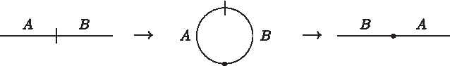
This definition is equivalent to the one given by Yancopoulos et al. (2005) and Bergeron et al. (2006). A more intuitive interpretation of, for example, (a), is that the event cuts both adjacencies {p, q} and {r, s} in G1 and replaces them with the adjacencies {p, r} and {q, s} in G2.
Note that an event that satisfies one of the conditions (b)-(d) of the dcj model only cuts the genome in one place. These events define the submodel of dcj called single-cut and join (scj), which we will study in Section 8. We will also consider restrictions of models so that they only deal with linear, circular, and/or uni-chromosomal genomes:
Definition 3
Given a model M, let
\documentclass{aastex}\usepackage{amsbsy}\usepackage{amsfonts}\usepackage{amssymb}\usepackage{bm}\usepackage{mathrsfs}\usepackage{pifont}\usepackage{stmaryrd}\usepackage{textcomp}\usepackage{portland, xspace}\usepackage{amsmath, amsxtra}\pagestyle{empty}\DeclareMathSizes{10}{9}{7}{6}\begin{document}$$M_{\rm lin} = \{ (G_1 , G_2) \mid (G_1 , G_2) \in M \ and \ G_1 \ and \ G_2 \ are \ linear \} .$$\end{document}
\documentclass{aastex}\usepackage{amsbsy}\usepackage{amsfonts}\usepackage{amssymb}\usepackage{bm}\usepackage{mathrsfs}\usepackage{pifont}\usepackage{stmaryrd}\usepackage{textcomp}\usepackage{portland, xspace}\usepackage{amsmath, amsxtra}\pagestyle{empty}\DeclareMathSizes{10}{9}{7}{6}\begin{document}$$M_{\rm uni} = \{ (G_1 , G_2) \mid (G_1 , G_2) \in M \ and \ G_1 \ and \ G_2 \ are \ uni \hbox{- }chromosomal \} .$$\end{document}
\documentclass{aastex}\usepackage{amsbsy}\usepackage{amsfonts}\usepackage{amssymb}\usepackage{bm}\usepackage{mathrsfs}\usepackage{pifont}\usepackage{stmaryrd}\usepackage{textcomp}\usepackage{portland, xspace}\usepackage{amsmath, amsxtra}\pagestyle{empty}\DeclareMathSizes{10}{9}{7}{6}\begin{document}$$M_{\rm circ} = \{ (G_1 , G_2) \mid (G_1 , G_2) \in M \ and \ G_1 \ and \ G_2 \ are \ circular \} .$$\end{document}
There are many questions one can ask within any model, including sorting, distance, median, halving, or aliquoting. We will focus on the sorting and distance problems here:
Definition 4 (Sorting Sequence and Distance)
A sequence of events\documentclass{aastex}\usepackage{amsbsy}\usepackage{amsfonts}\usepackage{amssymb}\usepackage{bm}\usepackage{mathrsfs}\usepackage{pifont}\usepackage{stmaryrd}\usepackage{textcomp}\usepackage{portland, xspace}\usepackage{amsmath, amsxtra}\pagestyle{empty}\DeclareMathSizes{10}{9}{7}{6}\begin{document}$$R_2 , \ldots , R_m$$\end{document}sorts G1into G2if\documentclass{aastex}\usepackage{amsbsy}\usepackage{amsfonts}\usepackage{amssymb}\usepackage{bm}\usepackage{mathrsfs}\usepackage{pifont}\usepackage{stmaryrd}\usepackage{textcomp}\usepackage{portland, xspace}\usepackage{amsmath, amsxtra}\pagestyle{empty}\DeclareMathSizes{10}{9}{7}{6}\begin{document}$$G_2 = R_m (\ldots (R_1 (G_1)))$$\end{document}. The sorting distance between G1and G2under a model\documentclass{aastex}\usepackage{amsbsy}\usepackage{amsfonts}\usepackage{amssymb}\usepackage{bm}\usepackage{mathrsfs}\usepackage{pifont}\usepackage{stmaryrd}\usepackage{textcomp}\usepackage{portland, xspace}\usepackage{amsmath, amsxtra}\pagestyle{empty}\DeclareMathSizes{10}{9}{7}{6}\begin{document}$${\mathcal R}$$\end{document}, denoted by\documentclass{aastex}\usepackage{amsbsy}\usepackage{amsfonts}\usepackage{amssymb}\usepackage{bm}\usepackage{mathrsfs}\usepackage{pifont}\usepackage{stmaryrd}\usepackage{textcomp}\usepackage{portland, xspace}\usepackage{amsmath, amsxtra}\pagestyle{empty}\DeclareMathSizes{10}{9}{7}{6}\begin{document}$$d_{\mathcal R} (G_1 , G_2)$$\end{document}, is the length of a shortest sorting sequence such that all Ri are\documentclass{aastex}\usepackage{amsbsy}\usepackage{amsfonts}\usepackage{amssymb}\usepackage{bm}\usepackage{mathrsfs}\usepackage{pifont}\usepackage{stmaryrd}\usepackage{textcomp}\usepackage{portland, xspace}\usepackage{amsmath, amsxtra}\pagestyle{empty}\DeclareMathSizes{10}{9}{7}{6}\begin{document}$${\mathcal R}$$\end{document}events. If such a sequence does not exist then we say\documentclass{aastex}\usepackage{amsbsy}\usepackage{amsfonts}\usepackage{amssymb}\usepackage{bm}\usepackage{mathrsfs}\usepackage{pifont}\usepackage{stmaryrd}\usepackage{textcomp}\usepackage{portland, xspace}\usepackage{amsmath, amsxtra}\pagestyle{empty}\DeclareMathSizes{10}{9}{7}{6}\begin{document}$$d_{\mathcal R} (G_1 , G_2) = \infty$$\end{document}. We say an\documentclass{aastex}\usepackage{amsbsy}\usepackage{amsfonts}\usepackage{amssymb}\usepackage{bm}\usepackage{mathrsfs}\usepackage{pifont}\usepackage{stmaryrd}\usepackage{textcomp}\usepackage{portland, xspace}\usepackage{amsmath, amsxtra}\pagestyle{empty}\DeclareMathSizes{10}{9}{7}{6}\begin{document}$${\mathcal R}$$\end{document}-event R is\documentclass{aastex}\usepackage{amsbsy}\usepackage{amsfonts}\usepackage{amssymb}\usepackage{bm}\usepackage{mathrsfs}\usepackage{pifont}\usepackage{stmaryrd}\usepackage{textcomp}\usepackage{portland, xspace}\usepackage{amsmath, amsxtra}\pagestyle{empty}\DeclareMathSizes{10}{9}{7}{6}\begin{document}$${\mathcal R}$$\end{document}-sorting with respect to G1and G2if\documentclass{aastex}\usepackage{amsbsy}\usepackage{amsfonts}\usepackage{amssymb}\usepackage{bm}\usepackage{mathrsfs}\usepackage{pifont}\usepackage{stmaryrd}\usepackage{textcomp}\usepackage{portland, xspace}\usepackage{amsmath, amsxtra}\pagestyle{empty}\DeclareMathSizes{10}{9}{7}{6}\begin{document}$$d_{\mathcal R} (R (G_1) , G_2) = d_{\mathcal R} (G_1 , G_2) - 1$$\end{document}.
Given two genomes, we can either find a shortest sorting sequence or just the sorting distance. Since the number of possible events in each step is polynomial, if we have a polynomial time algorithm for distance, then we also have one for sorting (Hannenhalli and Pevzner, 1999). That is why when discussing poly-time complexity, we will focus only on the distance problem. Note however that the precise complexities may differ, as for example is the case for the reversal model, where the distance can be computed in linear time (Bader et al., 2001) while the best-known sorting algorithms have worst-case time complexity \documentclass{aastex}\usepackage{amsbsy}\usepackage{amsfonts}\usepackage{amssymb}\usepackage{bm}\usepackage{mathrsfs}\usepackage{pifont}\usepackage{stmaryrd}\usepackage{textcomp}\usepackage{portland, xspace}\usepackage{amsmath, amsxtra}\pagestyle{empty}\DeclareMathSizes{10}{9}{7}{6}\begin{document}$$O (n^{3 / 2} \sqrt{\log n})$$\end{document} (Tannier et al., 2007).
4. Submodels of Double-Cut and Join
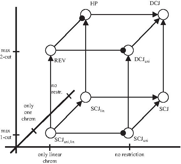
Motivated by the variety of biological systems, many distinct rearrangement models have been studied. These models differ in several aspects, spanning a whole space of genome rearrangement models. The three most relevant dimensions of this space are (i) the number of chromosomes a genome may have, (ii) the shape that the chromosomes may have (i.e., linear or circular), and (iii) the maximum number of chromosome cuts (and joins) an operation may perform.3 This three-dimensional space is visualized in Figure 1. Each of the corners of the cube are formally defined by deriving a submodel from either dcj or scj using the linear and/or uni-chromosomal restrictions. For example, hp = dcjlin. One can also think of these models in terms of the operations they allow, which is shown in Table 1.
The space of dcj genome rearrangement submodels and their relationships, as given in Sections 5 and 6. Not shown in the cube are circular-only models, which are the topic of Section 7. An arrow on an edge from M to M′ indicates that M′ is stronger than M. An edge between M and M′ with a circular ending at M′ indicates that M′ and M are weakly-equivalent, though there are genomes sortable under M′ but not under M.
Models and Elementary Operations
Model
Operation
dcj
hp
scj
scjlin
(scjuni)lin
proper translocation
•
•
semi translocation
•
•
•
•
path fission fusion
•
•
•
•
excision integration
•
reversal
•
•
○
○
○
circularization linearization
•
•
cycle fission fusion
•
○
A Description of Some of the Models in Terms of the Elementary Operations Defined by Bergeron et al. (2006). A dark bullet means that the operation is fully contained in the model, no bullet means that the operation is disjoint with the model, and an empty bullet means that some but not all of the operation is contained in the model. Furthermore, each model is precisely the union of the operations specified by the bullets.
Of the corners of the cube visualized in Figure 1, some are of particular interest and thus have been studied more than others. The first model to be studied was the rev model, where the only allowed operation was the reversal. The biological motivation for this model goes back to Nadeau and Taylor (1984) and it was first formally modeled by Sankoff (1992). The first polynomial-time algorithm for computing the reversal distance and solving the reversal model was given by Hannenhalli and Pevzner (1995b). In the same year, Hannenhalli and Pevzner (1995a) also looked at a model where multiple linear chromosomes are allowed, as is often the case in eukaryotic genomes. After its authors, the resulting model is called the hp model. A combination of work showed that the distance under hp can be computed in poly-time (Hannenhalli and Pevzner, 1995a; Tesler, 2002; Ozery-Flato and Shamir, 2003; Jean and Nikolski, 2007; Bergeron et al., 2009).
A more recently introduced model is the double-cut and join (dcj), which encompasses all events that can be achieved by first cutting the genome in up to two places, and then rejoining them in different combinations (Yancopoulos et al., 2005). Though such a model is less biologically realistic than the hp model, there are fast algorithms for solving it (Bergeron et al., 2006) which have made it useful as an efficient approximation for the hp distance (Adam and Sankoff, 2008; Lin and Moret, 2008; Mixtacki, 2008). The dcj model is a superset of all the other models in the cube, and is thus the most general.
The rev, hp, and dcj models are all double-cut models, in that they allow for the cutting of the genome in two places. However, one can also consider models where only one cut is allowed. These make up the bottom plane of the cube, with the most general of these being the already defined scj model. These models have not yet been studied, since they are quite restrictive. However, we became aware of their relevance when we looked at certain rearrangement scenarios in eukaryotic evolution. In particular, while studying rearrangement scenarios between human and mouse with a minimum number of breakpoint reuses, Bergeron et al. (2008) observed that most of the events (213 out of 246) were single-cut (186 semi-translocations and affix reversals, 15 fissions and 12 fusions). This observation raised our interest in studying scj and its submodels.
In Section 8, we give a linear time algorithm for the sorting distance in the scj model. When restricted to linear chromosomes (scjlin), we have the single-cut equivalent of the hp model, allowing fissions, fusions, semi-translocations, and affix reversals. The complexity of this model is unknown. The even more restrictive (scjuni)lin model consists of only affix reversals, which reverse a prefix/suffix of a chromosome, and is the single-cut equivalent of the rev model. There is a simple 2-approximation algorithm for the sorting distance, which increases the number of short cycles by at least one every two steps. However, the complexity of the problem remains open. It is related to the problem of sorting burnt pancakes (Gates and Papadimitiou, 1979; Cohen and Blum, 1995), which is similar except that the chromosome has an orientation and only prefix reversals are allowed. The complexity of this problem is also open.
5. Sorting Distance Relationships
In this section, we study the relationship between sorting distances under the various models represented in the cube of Figure 1. For example, if you compare two models that are connected by an edge of the cube, then the one that is furthest from the origin is, in some sense, at least as strong as the closer one. Some models, however, are strictly stronger than others. Of course, it is clear from the definitions that, for example, a multi-chromosomal genome can be sorted by scj and cannot be sorted by scjuni. However, we are interested if there are genomes which can be sorted by both models, but with fewer steps in one than the other. Formally, we define:
Definition 5 (Strong)
A model M is as strong as a model M′ if for all genomes G1and G2, dM(G1,G2) ≤ dM′(G1, G2). Furthermore, M is stronger than M′ if it is as strong as M′ and there exist two genomes G1and G2such that dM(G1, G2) <dM′(G1, G2)<∞.
We start with an easy observation and its immediate corollary:
Lemma 1 (Submodel Lemma)
For any two models,\documentclass{aastex}\usepackage{amsbsy}\usepackage{amsfonts}\usepackage{amssymb}\usepackage{bm}\usepackage{mathrsfs}\usepackage{pifont}\usepackage{stmaryrd}\usepackage{textcomp}\usepackage{portland, xspace}\usepackage{amsmath, amsxtra}\pagestyle{empty}\DeclareMathSizes{10}{9}{7}{6}\begin{document}$$M^{\prime} \subseteq M$$\end{document}if and only if M is as strong as M′.
Proof
For the only if direction it is enough to observe that any sorting sequence under M′ is by definition also a sorting sequence under M. For the if direction, let (G1, G2) be an element of M′. Then, dM(G1, G2) = dM′(G1, G2) = 1, and hence \documentclass{aastex}\usepackage{amsbsy}\usepackage{amsfonts}\usepackage{amssymb}\usepackage{bm}\usepackage{mathrsfs}\usepackage{pifont}\usepackage{stmaryrd}\usepackage{textcomp}\usepackage{portland, xspace}\usepackage{amsmath, amsxtra}\pagestyle{empty}\DeclareMathSizes{10}{9}{7}{6}\begin{document}$$(G_1, G_2) \in M$$\end{document}. ▪
Corollary 2
dcjis as strong asscj, and for all models M, M is as strong as Mlinand Muni.
We first study if the restriction to linear or uni-chromosomal genomes makes the dcj or scj models stronger.
Let G1 = (1, 3, 2) and G2 = (1, 2, 3). Since Corollary 2 shows that “as strong as” already holds for each of the above relationships, it suffices to show that
We can sort G1 into G2 using two scj events. First, we make an excision by replacing points {1h, 3t} and {2h} with {1h} and {2h, 3t}. Second, we make an integration by replacing points {1h} and {3h, 2t} with {1h, 2t} and {3h}. However, there does not exist a sorting sequence of length two under either scjlin, scjuni, or dcjuni models, though the genomes are clearly sortable under all these models. ▪
To complete the picture, it is already known that there are genomes that are sortable in hp but require more steps than in dcj (for an example, see Bergeron et al., 2009), so dcj is stronger than hp.
We next look if the flexibility of double-cut operations makes the models in the top plane more powerful than their respective counterparts in the bottom plane. There is a simple example that answers this question in the affirmative.
Lemma 4
We have that
revis stronger than (scjuni)lin
hpis stronger thanscjlin
dcjuniis stronger thanscjuni
dcjis stronger thanscj.
Proof
Let G1 = (1, −2, 3) and G2 = (1, 2, 3). The Submodel Lemma shows that “as strong as” already holds for each of the above relationships, so it suffices to show that
We can sort G1 into G2 using just one event in the rev model, while there is no single scj event that does this. However, G1 is sortable into G2 using affix reversals (i.e. (scjuni)lin). The lemma follows by applying the Submodel Lemma.
We now compare (scjuni)lin with scjlin and show that the flexibility to create additional chromosomes in intermediate steps adds power when we are restricted to single-cut operations and linear genomes.
Lemma 5
scjlinis stronger than (scjuni)lin.
Proof
Corollary 2 implies scjlin is as strong as (scjuni)lin. We show that for genomes G1 = (1, −2, −3, 4) and G2 = (1, 2, 3, 4),
\documentclass{aastex}\usepackage{amsbsy}\usepackage{amsfonts}\usepackage{amssymb}\usepackage{bm}\usepackage{mathrsfs}\usepackage{pifont}\usepackage{stmaryrd}\usepackage{textcomp}\usepackage{portland, xspace}\usepackage{amsmath, amsxtra}\pagestyle{empty}\DeclareMathSizes{10}{9}{7}{6}\begin{document}\begin{align*}d_{\hbox{\sc scj}_{\rm lin}} (G_1 , G_2) < d_{(\hbox{\sc scj}_{\rm uni}) _{\rm lin}} (G_1 , G_2) < \infty.\end{align*}\end{document}
There exists a sorting sequence of length 4 under scjlin that makes a fission between −2 and −3, two affix reversals of genes 2 and 3, respectively, and a final fusion. However, one can verify that using only affix reversals the sorting distance is at least five, while six affix reversals suffice. ▪
In some cases, however, additional flexibility does not make a model stronger. Consider the scjuni model, which differs from the (scjuni)lin model in that, besides affix reversals, it allows the circularization and linearization of the chromosome. This obviously allows sorting a linear chromosome into a circular one, something that (scjuni)lin does not allow. However, for genomes that are sortable under both models, we will show that circularization/linearization cannot help to decrease the distance. We capture this relationship using the following definition:
Definition 6 (Weak Equivalence)
Two models M and M′ are weakly equivalent if, for all genomes G1and G2, if dM(G1, G2) < ∞ and dM′(G1, G2) < ∞ , then dM(G1, G2) = dM′(G1, G2).
We now study the models of Figure 1 which are weakly equivalent. We prove that circularizations and linearizations in a uni-chromosomal environment do not add power to either the scj or the dcj models.
Lemma 6
scjuniand (scjuni)linare weakly equivalent.
Proof
The condition that G1 is sortable into G2 under both scjuni and (scjuni)lin is equivalent to the condition that G1 and G2 are both uni-chromosomal linear genomes. We thus need to show that for two such genomes,
\documentclass{aastex}\usepackage{amsbsy}\usepackage{amsfonts}\usepackage{amssymb}\usepackage{bm}\usepackage{mathrsfs}\usepackage{pifont}\usepackage{stmaryrd}\usepackage{textcomp}\usepackage{portland, xspace}\usepackage{amsmath, amsxtra}\pagestyle{empty}\DeclareMathSizes{10}{9}{7}{6}\begin{document}\begin{align*}d_{\hbox{\sc scj}_{\rm uni}} (G_1 , G_2) = d_{(\hbox{\sc scj}_{\rm uni}) _{\rm lin}} (G_1 , G_2).\end{align*}\end{document}
We show that for any optimal scjuni sorting sequence that creates a circular chromosome in an intermediate step, there exists a sorting sequence of equal length without a circular chromosome. Since the only scj operation that can be performed on a uni-chromosomal circular genome is to linearize it, we know that every circularization is immediately followed by a linearization. Thus, w.l.o.g. the situation can be described as an exchange of a prefix A and a suffix B:
However, the same effect can be achieved by two affix reversals, namely first reversing A and then B:
▪
A similar situation occurs when we add circularization and linearization to the reversal model, though the proof is more involved:
Lemma 7
dcjuniandrevare we weakly equivalent
Proof
The condition that G1 is sortable into G2 under both dcjuni and rev is equivalent to the condition that G1 and G2 are both uni-chromosomal linear genomes. We need to show that for this type of genomes,
\documentclass{aastex}\usepackage{amsbsy}\usepackage{amsfonts}\usepackage{amssymb}\usepackage{bm}\usepackage{mathrsfs}\usepackage{pifont}\usepackage{stmaryrd}\usepackage{textcomp}\usepackage{portland, xspace}\usepackage{amsmath, amsxtra}\pagestyle{empty}\DeclareMathSizes{10}{9}{7}{6}\begin{document}\begin{align*}d_{\hbox{\sc dcj}_{\rm uni}} (G_1 , G_2) = d_{\hbox{\sc rev}} (G_1 , G_2).\end{align*}\end{document}
Consider an optimal dcjuni sorting sequence S that has the smallest possible number of circularizations. We show, by contradiction, that this number is zero, proving the lemma. Let L be the genome prior to the first circularization, let C be the one right after it, let C′ be the genome right before the first linearization, and let L′ be the one right after it. Let d be the length of the sorting sequence between C and C′ (these must be reversals).
We will apply Theorem 3.2 from Meidanis et al. (2000), which states that the reversal distance between any two circular chromosomes (C and C′ in our case) is the same as the reversal distance between their linearizations, if they share a telomere. If L and L′ share a telomere, then there is a sorting sequence with shorter length that replaces d + 2 events between them with d reversals, which contradicts the optimality of S.
Suppose w.l.o.g that the two telomeres of L are {p} and {s}, that {q} is a telomere in L′, that {q,r} is an adjacency in L, and p, q, r, s are ordered in L. We can perform two reversals on L, the first one replacing {p} and {q,r} with {q} and {p,r}, and the second replacing {p,r} and {s} with {p,s} and {r}. The effect on the genome graph can be visualized as follows:
Note that circularizing the resulting genome, L″ yields genome C, and L″ shares a telomere with L′. Therefore, by the theorem, there exist d reversals that sort L″ into L′. We can then get a new sorting sequence that replaces the d + 2 events between L and L′ with the two reversals described above followed by d reversals given by the theorem of Meidanis et al. (2000). This sorting sequence has the same length as S but has one less circularization, a contradiction. ▪
The results of this section are compactly summarized in Figure 1 by marking the endpoints on the edges of the cube. There remains one edge whose relationship we have not yet categorized, which is the question of whether the hp model is stronger than the rev model, or, in other words, whether there exist uni-chromosomal linear genomes that require less steps to sort under hp than under rev. In Section 6, we will prove that the two models are weakly equivalent. Note that this is not trivial, because under hp we can split chromosomes in intermediate steps, which proved to make scjlin stronger than (scjuni)lin (Lemma 5). In fact, the weak equivalence of hp and rev is a curious asymmetry in the cube, since the power to create multiple chromosomes in intermediate steps makes all the other models in the back plane stronger than their counterparts in the front.
The Submodel Lemma implies other results which we have not explicitly stated but that can be deduced by looking at the transitive relationship between the edges. For instance, there are genomes that are sortable under scjuni that require less steps under scjlin. Additionally some models which are not subsets of each other (like scj and hp) are incomparable. That is, there are genomes that are sortable under scj but require less steps under hp, and there are other genomes for which the opposite holds. The examples of (1, 3, 2) and (1, −2, 3) are sufficient to prove incomparability of scj with rev and with hp.
6. The hp and rev Models are Weakly Equivalent
There has been a rich theory developed to study sorting distances under hp which we will make use of in this section (Bergeron et al., 2009). One of its main results is that when sorting A into B, one should consider the case of whether A contains a so-called unoriented component or not. When there is an unoriented component, there is always an hp-sorting event that is a translocation or a reversal (if the genome is uni-chromosomal this must be a reversal). In the other case, the hp distance turns out to be exactly the dcj distance, which has been completely characterized in terms of the effect of sorting operations on the adjacency graph AG(A, B). Formally, we can restate the known results as follows:
Lemma 8
(Bergeron et al., 2009, 2006). Let A and B be two uni-chromosomal genomes sortable in thehpmodel. At least one of the following holds:
(a) There exists a reversal which ishp-sorting from A to B.
(b) For anyhp-event, we have that it ishp-sorting from A to B if and only if it either increases the number of cycles in AG(A,B) by one or the number of odd paths by two.
Lemma 8 now allows us to prove the main theorem that hp and rev are weakly equivalent. Our approach is to show that one can in all cases find a reversal which is hp-sorting.
Theorem 9
For any two uni-chromosomal linear genomes A and B,\documentclass{aastex}\usepackage{amsbsy}\usepackage{amsfonts}\usepackage{amssymb}\usepackage{bm}\usepackage{mathrsfs}\usepackage{pifont}\usepackage{stmaryrd}\usepackage{textcomp}\usepackage{portland, xspace}\usepackage{amsmath, amsxtra}\pagestyle{empty}\DeclareMathSizes{10}{9}{7}{6}\begin{document}\begin{align*}d_{\hbox{\sc hp}} (A,B) = d_{\hbox{\sc rev}} (A,B).\end{align*}\end{document}
Proof
It is sufficient to show that there exists a reversal-event on A that is hp-sorting. Assume for the sake of contradiction that property (a) of Lemma 8 does not hold and there is no such reversal. Then any hp-sorting event from A to B must be a fission, since all other hp events require multiple chromosomes. Denote by F such a fission-event. The effect of a fission on the adjacency graph AG(A, B) is to either turn a cycle into an even path or split a path in two. Since a fission can never increase the number of cycles, property (b) of Lemma 8 implies that F increases the number of odd paths by two. This can only happen if the vertex split by F lies on an even path, and, therefore, the adjacency graph must contain an even path. Since A and B are both uni-chromosomal linear, there are exactly four telomeres and hence exactly two paths. If one of the paths is even so must be the other one, and hence there must be one AA-path and one BB-path.
Let x = {p} be a telomere of A, let y = {q,r} be any A-adjacency that lies on the BB-path, and suppose without loss of generality that p, q, r are ordered. We can define an event that reverses the interval between x and y. Formally, let \documentclass{aastex}\usepackage{amsbsy}\usepackage{amsfonts}\usepackage{amssymb}\usepackage{bm}\usepackage{mathrsfs}\usepackage{pifont}\usepackage{stmaryrd}\usepackage{textcomp}\usepackage{portland, xspace}\usepackage{amsmath, amsxtra}\pagestyle{empty}\DeclareMathSizes{10}{9}{7}{6}\begin{document}$$R = (A, A \setminus \{ \{p\}, \{q, r\}\} \cup \{\{p, r\}, \{q\}\})$$\end{document}. The effect of R on the adjacency graph is to change the two even paths into two odd paths. Therefore, R is an hp-sorting reversal-event by property (b) of Lemma 8, contradicting our assumption that property (a) does not hold. ▪
7. Circular-Only Models
In this section, we consider restricting dcj and its sub-models so that they only contain circular chromosomes. As with linearity, we consider the effects of the circularity restriction in combination with the other two dimensions of the cube of Figure 1: the number of chromosomes and the number of allowed cuts. First, we consider the restriction of circularity on the full dcj model, and show that when the initial and final genomes are circular, no optimal dcj sorting sequence will contain any linear chromosomes.
Lemma 10
Let A and B be two circular genomes, and let R be adcj-sorting event on A. Then\documentclass{aastex}\usepackage{amsbsy}\usepackage{amsfonts}\usepackage{amssymb}\usepackage{bm}\usepackage{mathrsfs}\usepackage{pifont}\usepackage{stmaryrd}\usepackage{textcomp}\usepackage{portland, xspace}\usepackage{amsmath, amsxtra}\pagestyle{empty}\DeclareMathSizes{10}{9}{7}{6}\begin{document}$$R \in \hbox{\sc dcj}_{\rm circ}$$\end{document}.
Proof
Since circular genomes do not contain any telomeres, R cannot act on telomeres of A, and so either case (a) or case (d) of Definition 2 holds. Suppose for the sake of contradiction that case (d) holds, and that an adjacency {p, q} is replaced by two telomeres {p} and {q}. Because all the connected components of AG (A, B) are cycles and not paths, the effect of R is to replace a cycle by an even path. The distance under the dcj model (Bergeron et al., 2006) is
\documentclass{aastex}\usepackage{amsbsy}\usepackage{amsfonts}\usepackage{amssymb}\usepackage{bm}\usepackage{mathrsfs}\usepackage{pifont}\usepackage{stmaryrd}\usepackage{textcomp}\usepackage{portland, xspace}\usepackage{amsmath, amsxtra}\pagestyle{empty}\DeclareMathSizes{10}{9}{7}{6}\begin{document}\begin{align*}d_{\hbox{\sc dcj}} (A, B) = \mid N (A) \mid - I(A, B)/2 - C_s(A,B) - C_l(A, B) .\end{align*}\end{document}
Therefore, R actually increases the dcj distance and cannot be dcj-sorting, a contradiction. Hence, case (a) must hold, and since in this case R(A) \ A does not contain any telomeres, R(A) is also a circular genome. ▪
Corollary 11
dcjcircanddcjare weakly equivalent.
Corollary 12
(dcjuni)circanddcjuniare weakly equivalent.
As far as applying the circularity restriction to the scj model, observe that any scj-event defined on a circular genome destroys circularity of one chromosome; thus, scjcirc = ∅.
8. Single-Cut and Join
We have already motivated the study of the sorting distance under the scj model, and in this section we give a linear time algorithm to compute it. Let A and B be two arbitrary genomes with the same underlying set of genes, N. We will use the following potential function in our analysis:
\documentclass{aastex}\usepackage{amsbsy}\usepackage{amsfonts}\usepackage{amssymb}\usepackage{bm}\usepackage{mathrsfs}\usepackage{pifont}\usepackage{stmaryrd}\usepackage{textcomp}\usepackage{portland, xspace}\usepackage{amsmath, amsxtra}\pagestyle{empty}\DeclareMathSizes{10}{9}{7}{6}\begin{document}\begin{align*}\Phi (A, B) = \mid N \mid - I (A, B)/2 - C_s(A, B) + C_l (A, B).\end{align*}\end{document}
First, we show that the potential function is 0 if and only if the two genomes are the same:
Lemma 13
A = B if and only if Φ(A, B) = 0.
Proof
The only if direction follows trivially from the definition of the adjacency graph. The if direction follows from a simple counting argument. Let a be the number of adjacencies in A, and t be the number of telomeres. By definition, a + t/2 = |N|. Since each short cycle accounts for one adjacency of A, and each odd path accounts for one telomere of A, we have that Cs(A, B) + I(A, B)/2 ≤ a + t/2 = |N|. Therefore, for the equality of the lemma to hold, we must have Cl(A, B) = 0, Cs(A, B) = a, and I(A, B) = t. Furthermore, since each of the a + t A-vertices is part of only one path or cycle (but not both) and each of the a cycles and t paths contains at least one vertex, the length of each path must be one. Since AG(A, B) contains only paths of length 1 and short cycles, we conclude that the points of A must be the same as the points of B. ▪
We can show using simple case analysis that Φ can decrease by at most one after any single event.
Lemma 14
For allscjevents R, Φ(R(A), B) − Φ(A, B) ≥ − 1.
Proof
We prove this statement for each of the three cases of the scj definition. Consider case (b) of the definition, where \documentclass{aastex}\usepackage{amsbsy}\usepackage{amsfonts}\usepackage{amssymb}\usepackage{bm}\usepackage{mathrsfs}\usepackage{pifont}\usepackage{stmaryrd}\usepackage{textcomp}\usepackage{portland, xspace}\usepackage{amsmath, amsxtra}\pagestyle{empty}\DeclareMathSizes{10}{9}{7}{6}\begin{document}$$B \cup \{ \{p, q \}, \{r \}\} = A \cup \{ \{p, r \}, \{q \}\}$$\end{document}. Suppose that {p, q} belong to a cycle in AG(A). The effect of the event on the adjacency graph is to combine a cycle and a path (the one ending in {r}) into a single path. The parity of the new path is the same as that of the old one because all cycles are even, so there is no change in the number of odd paths. Also, the number of long cycles decreased by at most one and the number of short cycles did not increase, proving the lower bound. If on the other hand, {p,q} belong to a path, then the effect of the event is interchange the parts of two paths. If the old paths had different parities, then so will the new ones, and if the old paths had the same parities, so will the new ones. Since no cycles are affected, this implies the lower bound.
Now consider case (c), where \documentclass{aastex}\usepackage{amsbsy}\usepackage{amsfonts}\usepackage{amssymb}\usepackage{bm}\usepackage{mathrsfs}\usepackage{pifont}\usepackage{stmaryrd}\usepackage{textcomp}\usepackage{portland, xspace}\usepackage{amsmath, amsxtra}\pagestyle{empty}\DeclareMathSizes{10}{9}{7}{6}\begin{document}$$B \cup \{ \{q\}, \{r\}\} = A \cup \{ \{q, r\} \} $$\end{document}. This has the effect of merging the vertices {q} and {r} in AG(A, B). If the vertices lie on the same path in AG(A, B), then the path must be even, and the new graph will have this path removed and one new cycle created, proving the lower bound. If the vertices lie on different paths, then the event has the effect of merging the two paths. Since this cannot increase the number of odd paths, the lower bound holds.
For the final case (d), \documentclass{aastex}\usepackage{amsbsy}\usepackage{amsfonts}\usepackage{amssymb}\usepackage{bm}\usepackage{mathrsfs}\usepackage{pifont}\usepackage{stmaryrd}\usepackage{textcomp}\usepackage{portland, xspace}\usepackage{amsmath, amsxtra}\pagestyle{empty}\DeclareMathSizes{10}{9}{7}{6}\begin{document}$$B \cup \{ \{q, r \} \} = A \cup \{ \{q \}, \{r \} \} $$\end{document}. The effect of the event is to split the vertex {q,r} in AG(A, B). If this vertex is part of a cycle, then the number of long cycles decreases by at most one, and the number of short cycles does not increase. Since the new path will be even, the lower bound holds.
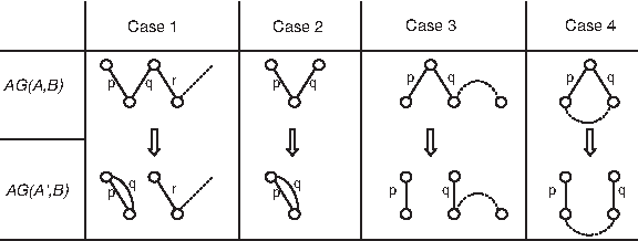
Combined with the fact that Φ cannot be negative, this gives a lower bound of Φ(A, B) on the sorting distance. We now consider Algorithm 1, whose cases are also illustrated in Figure 2. ▪
Algorithm for sorting under scj
whileA ≠ Bdo
if there exists an A-path P with length ≥ 3 then
Let p, q, r be the first three edges (from an arbitrary A end of P).
Let \documentclass{aastex}\usepackage{amsbsy}\usepackage{amsfonts}\usepackage{amssymb}\usepackage{bm}\usepackage{mathrsfs}\usepackage{pifont}\usepackage{stmaryrd}\usepackage{textcomp}\usepackage{portland, xspace}\usepackage{amsmath, amsxtra}\pagestyle{empty}\DeclareMathSizes{10}{9}{7}{6}\begin{document}$$A^{\prime} = A \setminus \{ \{p \}, \{q, r \} \} \cup \{ \{r \}, \{p, q \} \} $$\end{document}.
else if there exists an A-path P with length of 2 then
Algorithm 1 terminates and outputs anscjsorting sequence of length Φ(A, B).
Proof
First, we observe that one of the cases always applies since if A ≠ B then there must be at least one path of length greater than one or a long cycle. One can also verify that in each case, (A, A′) is an scj event. Finally, we show that Φ(A′, B) − Φ(A, B) = − 1:
Case 1: A short cycle is created and the length of P decreases by two.
Case 2: An even path (P) is removed and a short cycle is created.
Case 3: An even path (P) is replaced by two odd paths.
Case 4: A long cycle is replaced by an even path.
▪
Thus, we have
Theorem 16
dscj(A, B) = Φ(A, B) = |N| − I(A, B)/2 − Cs(A, B) + Cl(A, B).
Corollary 17
dscj(A, B) is computable in O(|N|) time.
Note the similarity to the formula for the dcj distance (Bergeron et al., 2006):
\documentclass{aastex}\usepackage{amsbsy}\usepackage{amsfonts}\usepackage{amssymb}\usepackage{bm}\usepackage{mathrsfs}\usepackage{pifont}\usepackage{stmaryrd}\usepackage{textcomp}\usepackage{portland, xspace}\usepackage{amsmath, amsxtra}\pagestyle{empty}\DeclareMathSizes{10}{9}{7}{6}\begin{document}\begin{align*}d_{\hbox{\sc dcj}} (A, B) = \mid N \mid - I(A, B)/2 - C_s(A, B) - C_l(A, B)\end{align*}\end{document}
Thus, the difference between the scj and dcj distances is 2Cl(A, B), i.e. twice the number of long cycles in the adjacency graph.
9. Experimental Results
We performed six different comparisons, all with respect to the human. In the first, we took the 281 synteny blocks of the mouse-human comparison done by Pevzner and Tesler (2003). In the other five, we used the 1359 synteny blocks of the chimp, rhesus monkey, mouse, rat, and dog used by Ma et al. (2006). For each comparison, we computed the scj, dcj, and hp distances. The hp distance was computed using GRIMM (Tesler, 2002). The results are shown in Table 2.
Rearrangement Distances under Different Models from Different Organisms to the Human
One immediately sees that the scj scenarios are far from parsimonious relative to the hp model. However, we stress that the goal of the scj model is to explore the importance of double-cut operations in evolution, and not to be a realistic evolutionary model. It can be an indicator of how many double-cut operations are really an advantage and how many are just an alternative that can be avoided. For example, consider that the difference between the hp and scj distances is 150% in the chimp-human comparison, and 60% in the mouse(Ma et al., 2006)-human comparison. This might suggest that somehow single-cut operations play a lesser part in the chimp-human evolution than in the mouse-human evolution. We also notice that the ratio of the scj to hp distance in the mouse-human comparison is much lower (1.2 vs. 1.6) using the synteny blocks of Pevzner and Tesler (2003) than using the synteny blocks of Ma et al. (2006). This suggests the sensitivity of this kind of breakpoint reuse analysis to synteny block partition.
In Section 5, we showed that there exist genomes for which the scj distance is smaller than the hp distance (for example 1,3,2). However, in all the experimental results, the hp distance is always much smaller. This suggests that the scj operations not allowed by hp, such as excisions, integrations, circularizations, and linearizations, are infrequent relative to fissions, fusions, translocations, and reversals.
10. Conclusion
In this article, we gave a formal set-theoretic definition of rearrangement models and operations, and used it to compare the power of various submodels of dcj with uni-chromosomal and/or linear/circular restrictions. We hope that the formal foundation for the notion of models will eventually lead to further insights into their relationships.
We also initiated the formal study of single-cut operations by giving a linear time algorithm for computing the distance under a new single-cut and join model. Many interesting algorithmic questions remain open, including the complexity of sorting using linear scj operations, and sorting using affix reversals.
Footnotes
Acknowledgments
P.M. would like to thank Allan Borodin and Michael Brudno for useful discussions. Most of the work was done while P.M. was a member of the International NRW Graduate School in Bioinformatics and Genome Research, and the AG Genominformatik group at Bielefeld, while being additionally funded by a German Academic Exchange Service (DAAD) Research Grant. P.M. gratefully acknowledges the support of these organizations. A preliminary version of some of these results appeared under the same title in RECOMB-CG (LNBI 5817, pp. 84–97, 2009).
Disclosure Statement
No competing financial interests exist.
1
Note that here scj refers to single-cut and join, as opposed to single-cut or join which was recently introduced by Feijão and Meidanis ().
2
Though this article focuses on genomes without duplicate genes, this definition could be extended to the more general case by treating the set of genes and its corresponding derivatives as multi-sets, including the genome.
3
In this article, we focus on double and single-cut operations. However, more general k-cut operations have also been considered (Alekseyev and Pevzner, ).
References
1.
AdamZ., SankoffD.2008. The ABCs of MGR with DCJ. Evol. Bioinform., 4:69–74.
2.
AlekseyevM.A., PevznerP.A.2007a. Are there rearrangement hotspots in the human genome?PLoS Comput. Biol., 3:e209.
3.
AlekseyevM.A., PevznerP.A.2007b. Whole genome duplications, multi-break rearrangements, and genome halving problem. Proc. SODA, 665–679.
4.
BaderD.A., MoretB.M.E., YanM.2001. A linear-time algorithm for computing inversion distance between signed permutations with an experimental study. J. Comput. Biol., 8:483–491.
5.
BergeronA., MixtackiJ., StoyeJ.2006. A unifying view of genome rearrangements. Lect. Notes Bioinform., 4175:163–173.
6.
BergeronA., MixtackiJ., StoyeJ.2008. On computing the breakpoint reuse rate in rearrangement scenarios. Lect. Notes Bioinform., 5267:226–240.
7.
BergeronA., MixtackiJ., StoyeJ.2009. A new linear time algorithm to compute the genomic distance via the double cut and join distance. Theor. Comput. Sci., 410:5300–5316.
8.
CohenD.S., BlumM.1995. On the problem of sorting burnt pancakes. Discr. Appl. Math., 61:105–120.
9.
DobzhanskyT., SturtevantA.H.1938. Inversions in the chromosomes of Drosophila Pseudoobscura. Genetics, 23:28–64.
10.
FeijãoP., MeidanisJ.2009. SCJ: A novel rearrangement operation for which sorting, genome median and genome halving problems are easy. Lect. Notes Bioinform., 5724:85–96.
11.
GatesW., PapadimitiouC.1979. Bounds for sorting by prefix reversals. Discr. Math., 27:47–57.
12.
HannenhalliS., PevznerP.A.1995a. Transforming men into mice (polynomial algorithm for genomic distance problem)Proc. FOCS 1995, 581–592.
13.
HannenhalliS., PevznerP.A.1995b. Transforming cabbage into turnip: polynomial algorithm for sorting signed permutations by reversals. Proc. STOC 1995, 178–189.
14.
HannenhalliS., PevznerP.A.1999. Transforming cabbage into turnip: polynomial algorithm for sorting signed permutations by reversals. J. ACM, 46:1–27.
15.
JeanG., NikolskiM.2007. Genome rearrangements: a correct algorithm for optimal capping. Inf. Process. Lett., 104:14–20.
16.
LinY., MoretB.M.E.2008. Estimating true evolutionary distances under the DCJ model. Bioinformatics, 24:i114–i122.
17.
MaJ., ZhangL., SuhB.B.et al.2006. Reconstructing contiguous regions of an ancestral genome. Genome Res., 16:1557–1565.
18.
MeidanisJ., WalterM.E.M.T., DiasZ.2000. Reversal distance of signed circular chromosomes. Technical report IC–00-23. Institute of Computing, University of Campinas.
NadeauJ.H., TaylorB.A.1984. Lengths of chromosomal segments conserved since divergence of man and mouse. Proc. Natl. Acad. Sci. USA, 81:814–818.
21.
Ozery-FlatoM., ShamirR.2003. Two notes on genome rearrangements. J. Bioinf. Comput. Biol., 1:71–94.
22.
PevznerP.A., TeslerG.2003. Transforming men into mice: the Nadeau-Taylor chromosomal breakage model revisited. Proc. RECOMB 2003, 247–256.
23.
SankoffD.1992. Edit distances for genome comparison based on non-local operations. Lect. Notes Comput. Sci., 644:121–135.
24.
SankoffD., TrinhP.2005. Chromosomal breakpoint reuse in genome sequence rearrangement. J. Comput. Biol., 12:812–821.
25.
SankoffD., CedergrenR., AbelY.1990. Genomic divergence through gene rearrangement. 428–438DoolittleR.F.Molecular Evolution: Computer Analysis of Protein and Nucleic Acid Sequences. Volume 183. Meth. Enzymol.Academic Press: San Diego.
26.
TannierE., BergeronA., SagotM.-F.2007. Advances on sorting by reversals. Discr. Appl. Math., 155:881–888.
27.
TeslerG.2002. Efficient algorithms for multichromosomal genome rearrangements. J. Comput. Syst. Sci., 65:587–609.
28.
YancopoulosS., AttieO., FriedbergR.2005. Efficient sorting of genomic permutations by translocation, inversion and block interchange. Bioinformatics, 21:3340–3346.