Methods for inferring species trees from sets of gene trees need to account for the possibility of discordance among the gene trees. Assuming that discordance is caused by incomplete lineage sorting, species tree estimates can be obtained by finding those species trees that minimize the number of “deep” coalescence events required for a given collection of gene trees. Efficient algorithms now exist for applying the minimizing-deep-coalescence (MDC) criterion, and simulation experiments have demonstrated its promising performance. However, it has also been noted from simulation results that the MDC criterion is not always guaranteed to infer the correct species tree estimate. In this article, we investigate the consistency of the MDC criterion. Using the multipscies coalescent model, we show that there are indeed anomaly zones for the MDC criterion for asymmetric four-taxon species tree topologies, and for all species tree topologies with five or more taxa.
1. Introduction
It is well known that, for a variety of reasons such as horizontal gene transfer, gene duplication and loss, and incomplete lineage sorting, gene trees can differ from each other and from the species tree along whose branches they have evolved (Degnan and Rosenberg, 2009; Maddison, 1997; Nichols, 2001). Consequently, methods for inferring species trees from sets of gene trees need to consider gene tree discordance in order to obtain reliable estimates.
Approaches to resolving the species tree/gene tree discordance problem in phylogenetic inference can be classified as either nonparametric (e.g., democratic vote, consensus, and parsimony-based) or parametric (e.g., likelihood and Bayesian). In general, nonparametric methods are faster than parametric methods, and hence they are computationally preferable for analyzing large datasets. One of the main concerns about these methods, however, is their potential for inconsistency. Under a specific model for the evolution of gene trees along the branches of species trees, a method is consistent if for each collection of values of the model parameters—the species tree topology and its branch lengths—the method produces a correct estimate of the species tree in the limit as the number of sampled gene trees goes to infinity. Recently, inconsistency results have been reported for several nonparametric methods, including democratic vote and several consensus methods. For example, Degnan and Rosenberg (2006) have shown that for asymmeric species trees with four leaves and for any species tree with at least five leaves, there exist species tree branch lengths such that the most likely gene tree topology under the multispecies coalescent model (Degnan and Rosenberg, 2009), the “democratic vote” topology, differs from the species tree topology. The greedy consensus method, which reconstructs the species tree by sequentially adding the most frequent clade compatible with all previously included clades, and which is not based specifically on coalescent principles, has also been proven to be inconsistent (Degnan et al., 2009). In contrast, several methods for inferring species trees from gene trees that make use of elements of the coalescent model, such as STAR (Liu et al., 2009), STEAC (Liu et al., 2009), and GLASS (Liu et al., 2010; Mossel and Roch, 2010), have been shown to be consistent under the multispecies coalescent model.
Maddison (1997) introduced a parsimony criterion for inferring species trees from gene trees by minimizing deep coalescences (MDC), and several exact algorithms and heuristics for implementing this criterion have recently been developed (Bansal et al., 2010; Than and Nakhleh, 2009). Unlike the democratic vote or greedy consensus methods, which provide algorithms for inferring species trees from collections of gene trees without taking into account the process by which the gene trees have been produced, the MDC criterion relies on an understanding of the specific nature of the way in which incomplete lineage sorting occurs. Thus, it is a natural candidate for species tree inference when discordance among gene trees is caused by incomplete lineage sorting. Simulation studies have suggested a high degree of accuracy of species tree estimates obtained by this criterion (Maddison and Knowles, 2006; Than and Nakhleh, 2009).
As noted by Than and Nakhleh (2009), however, it has been observed that in some cases, the MDC criterion does not reconstruct the correct species tree. As no theoretical results concerning consistency properties of the criterion have yet been reported, in this paper we investigate whether it is consistent under the multispecies coalescent model. We show that if gene lineages have evolved according to the multispecies coalescent model, then the MDC criterion is inconsistent. In other words, for certain combinations of species tree topologies and branch lengths, the MDC criterion infers an incorrect species tree topology in the limit as the number of sampled genes increases without bound.
2. The Minimizing-Deep-Coalescence Criterion
Although a variety of reasons can explain why gene trees can disagree with the species tree that contains them, we assume throughout this article that incomplete lineage sorting, or deep coalescence, is the only source for the discordance. Looking backward in time, the discordance between a gene tree and a species tree occurs because gene lineages can persist deeper than speciation events, providing opportunities for them to coalesce in an order different from the order of speciation events.
2.1. The deep coalescence cost
To measure the severity of the topological disagreement between a gene tree and a species tree, we use the deep coalescence cost, first introduced by Maddison (1997). Given a binary, rooted gene tree T and species tree S on a taxon set X, the deep coalescence cost for reconciling T within S is computed as follows. Each node v of T is mapped to its most recent common ancestor (MRCA) node in S, that is, the most recent node in S whose descendant leaf set (in S) contains all of the descendant leaves of v in T (Fig. 1). For each internal branch e of S, let xlS(T, e) be the number of gene lineages at the “top” of branch e minus 1; xlS(T, e) is also called the number of “extra” lineages in e. The deep coalescence cost for reconciling T within S is defined as
\documentclass{aastex}
\usepackage{amsbsy}
\usepackage{amsfonts}
\usepackage{amssymb}
\usepackage{bm}
\usepackage{mathrsfs}
\usepackage{pifont}
\usepackage{stmaryrd}
\usepackage{textcomp}
\usepackage{portland, xspace}
\usepackage{amsmath, amsxtra}
\pagestyle{empty}
\DeclareMathSizes {10} {9} {7} {6}
\begin{document}
\begin{align*}
\alpha (T , S) = \sum_{e \in \mathring{E}(S)} {\rm xl}_{S} (T , e),
\tag{2.1}
\end{align*}
\end{document}
where
\documentclass{aastex}
\usepackage{amsbsy}
\usepackage{amsfonts}
\usepackage{amssymb}
\usepackage{bm}
\usepackage{mathrsfs}
\usepackage{pifont}
\usepackage{stmaryrd}
\usepackage{textcomp}
\usepackage{portland, xspace}
\usepackage{amsmath, amsxtra}
\pagestyle{empty}
\DeclareMathSizes {10} {9} {7} {6}
\begin{document}
$${\mathop E \limits^ \circ} (S)$$\end{document} is the set of internal branches in S.
Computing the deep coalescence cost. Gene tree T is fitted onto species tree S according to a most recent common ancestor (MRCA) mapping. In the figure, mappings between leaves are omitted, and for clearer illustration of how T is reconciled within S, the MRCAs of the internal nodes of T are placed along the branches of S rather than at internal nodes of S. The labels u′, v′, and w′ refer to specific nodes of S. In this example, the minimizing-deep-coalescence (MDC) cost for T and S, α(T, S), is two, the total number of extra lineages in all the branches of S.
It is possible to compute the number of extra lineages in an internal branch e of S without using an MRCA mapping between the nodes of T and the nodes of S (Theorem 2 of Than and Nakhleh, 2009). For an internal branch e of the species tree S, let CS(e) be the label set of the leaves under e (i.e., CS(e) is the set of leaf labels for the cluster induced by e). A subtree t of T whose leaf set is contained in CS(e) is maximal with respect to e if it is not a proper subtree of another subtree t′ of T whose leaf set is also contained in CS(e). If k is the number of maximal subtrees of T with respect to e, then the number of extra lineages in e is
\documentclass{aastex}
\usepackage{amsbsy}
\usepackage{amsfonts}
\usepackage{amssymb}
\usepackage{bm}
\usepackage{mathrsfs}
\usepackage{pifont}
\usepackage{stmaryrd}
\usepackage{textcomp}
\usepackage{portland, xspace}
\usepackage{amsmath, amsxtra}
\pagestyle{empty}
\DeclareMathSizes {10} {9} {7} {6}
\begin{document}
\begin{align*}
{ \rm xl}_{S} ( T , e ) = k - 1. \tag{2.2}
\end{align*}
\end{document}
For example, Figure 1 illustrates that there is one extra lineage in the branch (u′, v′) of the species tree topology S. We can also obtain this result by noting that (u′, v′) induces the cluster of leaf labels C = {a, b, c, d}. There are two subtrees of T whose leaf sets are subsets of C, and that are maximal with respect to the branch (u′, v′): t1 = (a, (b, c)) and t2 = (d). Consequently, from Eq. (2.2) we obtain that the number of extra lineages in (u′, v′) is 1.
Suppose that we are given a collection G of binary, rooted gene trees on label set X. Denoting by R(X) the set of all possible binary, rooted trees on X, then for each candidate species tree S′ in R(X), we compute the deep coalescence cost for reconciling all gene trees in G within S′ by evaluating the sum
\documentclass{aastex}
\usepackage{amsbsy}
\usepackage{amsfonts}
\usepackage{amssymb}
\usepackage{bm}
\usepackage{mathrsfs}
\usepackage{pifont}
\usepackage{stmaryrd}
\usepackage{textcomp}
\usepackage{portland, xspace}
\usepackage{amsmath, amsxtra}
\pagestyle{empty}
\DeclareMathSizes {10} {9} {7} {6}
\begin{document}
\begin{align*}
\alpha ( G , S^{ \prime} ) = \sum_{T \in G} \alpha ( T , S^{ \prime} ) , \tag{2.3}
\end{align*}
\end{document}
where α(T, S′) is calculated using Eq. (2.1). Under the MDC criterion, a tree in R(X) whose deep coalescence cost, defined by Eq. (2.3), is the smallest among those of all trees in R(X) is taken as an estimate of the true species tree S. Note that more than one tree can be tied with the smallest deep coalescence cost, and in this case, the MDC criterion randomly chooses one of them as an estimate of S. Efficient algorithms exist for identifying optimal trees under the MDC criterion for a collection of gene trees (Bansal et al., 2010; Than and Nakhleh, 2009).
2.2. An observation about collections of deep coalescence costs
Given two trees in R(X) that have the same unlabeled topology,
\documentclass{aastex}
\usepackage{amsbsy}
\usepackage{amsfonts}
\usepackage{amssymb}
\usepackage{bm}
\usepackage{mathrsfs}
\usepackage{pifont}
\usepackage{stmaryrd}
\usepackage{textcomp}
\usepackage{portland, xspace}
\usepackage{amsmath, amsxtra}
\pagestyle{empty}
\DeclareMathSizes {10} {9} {7} {6}
\begin{document}
$$S_1^{\prime}$$\end{document} and
\documentclass{aastex}
\usepackage{amsbsy}
\usepackage{amsfonts}
\usepackage{amssymb}
\usepackage{bm}
\usepackage{mathrsfs}
\usepackage{pifont}
\usepackage{stmaryrd}
\usepackage{textcomp}
\usepackage{portland, xspace}
\usepackage{amsmath, amsxtra}
\pagestyle{empty}
\DeclareMathSizes {10} {9} {7} {6}
\begin{document}
$$S_2^{\prime}$$\end{document}, let us compare
\documentclass{aastex}
\usepackage{amsbsy}
\usepackage{amsfonts}
\usepackage{amssymb}
\usepackage{bm}
\usepackage{mathrsfs}
\usepackage{pifont}
\usepackage{stmaryrd}
\usepackage{textcomp}
\usepackage{portland, xspace}
\usepackage{amsmath, amsxtra}
\pagestyle{empty}
\DeclareMathSizes {10} {9} {7} {6}
\begin{document}
$$\{\alpha (T , S_1^{\prime}) \mid T \in R (X)\}$$\end{document} and
\documentclass{aastex}
\usepackage{amsbsy}
\usepackage{amsfonts}
\usepackage{amssymb}
\usepackage{bm}
\usepackage{mathrsfs}
\usepackage{pifont}
\usepackage{stmaryrd}
\usepackage{textcomp}
\usepackage{portland, xspace}
\usepackage{amsmath, amsxtra}
\pagestyle{empty}
\DeclareMathSizes {10} {9} {7} {6}
\begin{document}
$$\{\alpha (T , S_2^{\prime}) \mid T \in R (X)\}$$\end{document}, the collections of deep coalescence costs for reconciling all trees in R(X) within
\documentclass{aastex}
\usepackage{amsbsy}
\usepackage{amsfonts}
\usepackage{amssymb}
\usepackage{bm}
\usepackage{mathrsfs}
\usepackage{pifont}
\usepackage{stmaryrd}
\usepackage{textcomp}
\usepackage{portland, xspace}
\usepackage{amsmath, amsxtra}
\pagestyle{empty}
\DeclareMathSizes {10} {9} {7} {6}
\begin{document}
$$S_1^{\prime}$$\end{document} and
\documentclass{aastex}
\usepackage{amsbsy}
\usepackage{amsfonts}
\usepackage{amssymb}
\usepackage{bm}
\usepackage{mathrsfs}
\usepackage{pifont}
\usepackage{stmaryrd}
\usepackage{textcomp}
\usepackage{portland, xspace}
\usepackage{amsmath, amsxtra}
\pagestyle{empty}
\DeclareMathSizes {10} {9} {7} {6}
\begin{document}
$$S_2^{\prime}$$\end{document}, respectively. Because
\documentclass{aastex}
\usepackage{amsbsy}
\usepackage{amsfonts}
\usepackage{amssymb}
\usepackage{bm}
\usepackage{mathrsfs}
\usepackage{pifont}
\usepackage{stmaryrd}
\usepackage{textcomp}
\usepackage{portland, xspace}
\usepackage{amsmath, amsxtra}
\pagestyle{empty}
\DeclareMathSizes {10} {9} {7} {6}
\begin{document}
$$S_1^{\prime}$$\end{document} and
\documentclass{aastex}
\usepackage{amsbsy}
\usepackage{amsfonts}
\usepackage{amssymb}
\usepackage{bm}
\usepackage{mathrsfs}
\usepackage{pifont}
\usepackage{stmaryrd}
\usepackage{textcomp}
\usepackage{portland, xspace}
\usepackage{amsmath, amsxtra}
\pagestyle{empty}
\DeclareMathSizes {10} {9} {7} {6}
\begin{document}
$$S_2^{\prime}$$\end{document} have the same unlabeled topology, there exists a permutation π of the taxon set X such that the leaves of
\documentclass{aastex}
\usepackage{amsbsy}
\usepackage{amsfonts}
\usepackage{amssymb}
\usepackage{bm}
\usepackage{mathrsfs}
\usepackage{pifont}
\usepackage{stmaryrd}
\usepackage{textcomp}
\usepackage{portland, xspace}
\usepackage{amsmath, amsxtra}
\pagestyle{empty}
\DeclareMathSizes {10} {9} {7} {6}
\begin{document}
$$S_1^{\prime}$$\end{document} can be relabeled according to π to obtain
\documentclass{aastex}
\usepackage{amsbsy}
\usepackage{amsfonts}
\usepackage{amssymb}
\usepackage{bm}
\usepackage{mathrsfs}
\usepackage{pifont}
\usepackage{stmaryrd}
\usepackage{textcomp}
\usepackage{portland, xspace}
\usepackage{amsmath, amsxtra}
\pagestyle{empty}
\DeclareMathSizes {10} {9} {7} {6}
\begin{document}
$$S_2^{\prime}$$\end{document}. Denoting by π(T), for
\documentclass{aastex}
\usepackage{amsbsy}
\usepackage{amsfonts}
\usepackage{amssymb}
\usepackage{bm}
\usepackage{mathrsfs}
\usepackage{pifont}
\usepackage{stmaryrd}
\usepackage{textcomp}
\usepackage{portland, xspace}
\usepackage{amsmath, amsxtra}
\pagestyle{empty}
\DeclareMathSizes {10} {9} {7} {6}
\begin{document}
$$T \in R (X)$$\end{document}, the tree obtained from T by applying π to its leaves (so that by our choice of π,
\documentclass{aastex}
\usepackage{amsbsy}
\usepackage{amsfonts}
\usepackage{amssymb}
\usepackage{bm}
\usepackage{mathrsfs}
\usepackage{pifont}
\usepackage{stmaryrd}
\usepackage{textcomp}
\usepackage{portland, xspace}
\usepackage{amsmath, amsxtra}
\pagestyle{empty}
\DeclareMathSizes {10} {9} {7} {6}
\begin{document}
$$\pi (S_1^{\prime} ) = S_2^{\prime}$$\end{document}), we have the following facts:
If the leaves of both T and
\documentclass{aastex}
\usepackage{amsbsy}
\usepackage{amsfonts}
\usepackage{amssymb}
\usepackage{bm}
\usepackage{mathrsfs}
\usepackage{pifont}
\usepackage{stmaryrd}
\usepackage{textcomp}
\usepackage{portland, xspace}
\usepackage{amsmath, amsxtra}
\pagestyle{empty}
\DeclareMathSizes {10} {9} {7} {6}
\begin{document}
$$S_1^{\prime}$$\end{document} are relabeled using π, then the MRCA mapping between the nodes of T and
\documentclass{aastex}
\usepackage{amsbsy}
\usepackage{amsfonts}
\usepackage{amssymb}
\usepackage{bm}
\usepackage{mathrsfs}
\usepackage{pifont}
\usepackage{stmaryrd}
\usepackage{textcomp}
\usepackage{portland, xspace}
\usepackage{amsmath, amsxtra}
\pagestyle{empty}
\DeclareMathSizes {10} {9} {7} {6}
\begin{document}
$$S_1^{\prime}$$\end{document} remains unchanged, and hence
\documentclass{aastex}
\usepackage{amsbsy}
\usepackage{amsfonts}
\usepackage{amssymb}
\usepackage{bm}
\usepackage{mathrsfs}
\usepackage{pifont}
\usepackage{stmaryrd}
\usepackage{textcomp}
\usepackage{portland, xspace}
\usepackage{amsmath, amsxtra}
\pagestyle{empty}
\DeclareMathSizes {10} {9} {7} {6}
\begin{document}
$$\alpha (T , S_1^{\prime}) = \alpha (\pi (T) , \pi (S_1^{\prime})) = \alpha (\pi (T) , S_2^{\prime})$$\end{document}.
Because π is a permutation of X, π(T1) ≠ π(T2) if T1 ≠ T2. Moreover, because R(X) is the set of all rooted, binary trees on X,
\documentclass{aastex}
\usepackage{amsbsy}
\usepackage{amsfonts}
\usepackage{amssymb}
\usepackage{bm}
\usepackage{mathrsfs}
\usepackage{pifont}
\usepackage{stmaryrd}
\usepackage{textcomp}
\usepackage{portland, xspace}
\usepackage{amsmath, amsxtra}
\pagestyle{empty}
\DeclareMathSizes {10} {9} {7} {6}
\begin{document}
$$\{\pi (T) \mid T \in R (X)\}= R (X)$$\end{document}.
These facts imply that
\documentclass{aastex}
\usepackage{amsbsy}
\usepackage{amsfonts}
\usepackage{amssymb}
\usepackage{bm}
\usepackage{mathrsfs}
\usepackage{pifont}
\usepackage{stmaryrd}
\usepackage{textcomp}
\usepackage{portland, xspace}
\usepackage{amsmath, amsxtra}
\pagestyle{empty}
\DeclareMathSizes {10} {9} {7} {6}
\begin{document}
$$\{\alpha (T , S_1^{\prime}) \mid T \in R (X)\} $$\end{document} is equal to
\documentclass{aastex}
\usepackage{amsbsy}
\usepackage{amsfonts}
\usepackage{amssymb}
\usepackage{bm}
\usepackage{mathrsfs}
\usepackage{pifont}
\usepackage{stmaryrd}
\usepackage{textcomp}
\usepackage{portland, xspace}
\usepackage{amsmath, amsxtra}
\pagestyle{empty}
\DeclareMathSizes {10} {9} {7} {6}
\begin{document}
$$\{\alpha ( \pi ( T ) , S_2^{ \prime} ) \mid T \in R ( X ) \} $$\end{document}, which is in turn equal to
\documentclass{aastex}
\usepackage{amsbsy}
\usepackage{amsfonts}
\usepackage{amssymb}
\usepackage{bm}
\usepackage{mathrsfs}
\usepackage{pifont}
\usepackage{stmaryrd}
\usepackage{textcomp}
\usepackage{portland, xspace}
\usepackage{amsmath, amsxtra}
\pagestyle{empty}
\DeclareMathSizes {10} {9} {7} {6}
\begin{document}
$$\{\alpha ( T , S_2^{ \prime} ) \mid T \in R ( X ) \} $$\end{document}.
This observation can be further refined. Note that a tree in R(X) can never be transformed into another tree of different unlabeled topology simply by relabeling its leaves according to a permutation π of X. Therefore, if R(X) is partitioned into subsets
\documentclass{aastex}
\usepackage{amsbsy}
\usepackage{amsfonts}
\usepackage{amssymb}
\usepackage{bm}
\usepackage{mathrsfs}
\usepackage{pifont}
\usepackage{stmaryrd}
\usepackage{textcomp}
\usepackage{portland, xspace}
\usepackage{amsmath, amsxtra}
\pagestyle{empty}
\DeclareMathSizes {10} {9} {7} {6}
\begin{document}
$$R_1 , R_2 , \ldots$$\end{document} of trees having the same unlabeled topology, then for each
\documentclass{aastex}
\usepackage{amsbsy}
\usepackage{amsfonts}
\usepackage{amssymb}
\usepackage{bm}
\usepackage{mathrsfs}
\usepackage{pifont}
\usepackage{stmaryrd}
\usepackage{textcomp}
\usepackage{portland, xspace}
\usepackage{amsmath, amsxtra}
\pagestyle{empty}
\DeclareMathSizes {10} {9} {7} {6}
\begin{document}
$$i = 1 , 2 , \ldots , \{\pi ( T ) \mid T \in R_i \} = R_i$$\end{document}. Thus,
\documentclass{aastex}
\usepackage{amsbsy}
\usepackage{amsfonts}
\usepackage{amssymb}
\usepackage{bm}
\usepackage{mathrsfs}
\usepackage{pifont}
\usepackage{stmaryrd}
\usepackage{textcomp}
\usepackage{portland, xspace}
\usepackage{amsmath, amsxtra}
\pagestyle{empty}
\DeclareMathSizes {10} {9} {7} {6}
\begin{document}
$$\{\alpha ( T , S_1^{ \prime} ) \mid T \in R_i \} = \{ \alpha ( T , S_2^{ \prime} ) \mid T \in R_i \} $$\end{document} for any two tree topologies
\documentclass{aastex}
\usepackage{amsbsy}
\usepackage{amsfonts}
\usepackage{amssymb}
\usepackage{bm}
\usepackage{mathrsfs}
\usepackage{pifont}
\usepackage{stmaryrd}
\usepackage{textcomp}
\usepackage{portland, xspace}
\usepackage{amsmath, amsxtra}
\pagestyle{empty}
\DeclareMathSizes {10} {9} {7} {6}
\begin{document}
$$S_1^{ \prime}$$\end{document} and
\documentclass{aastex}
\usepackage{amsbsy}
\usepackage{amsfonts}
\usepackage{amssymb}
\usepackage{bm}
\usepackage{mathrsfs}
\usepackage{pifont}
\usepackage{stmaryrd}
\usepackage{textcomp}
\usepackage{portland, xspace}
\usepackage{amsmath, amsxtra}
\pagestyle{empty}
\DeclareMathSizes {10} {9} {7} {6}
\begin{document}
$$S_2^{ \prime}$$\end{document} that have the same unlabeled topology. This refined observation, that the collection of deep coalescence costs of all gene trees having a given unlabeled topology is dependent only on the species tree's unlabeled topology, is used in the next section in the proof of the inconsistency of the MDC criterion.
3. Inconsistency of the MDC Criterion
Let S be a binary, rooted species tree on a taxon label set X, and let λ be the vector of the lengths of branches of S. The branch lengths are positive, and are measured in coalescent time units. We assume that gene lineages have evolved along the branches of S following the multispecies coalescent model (Degnan and Rosenberg, 2009). We further assume that one gene lineage is sampled in each species, so that a gene tree and species tree have the same number of lineages, and that gene trees are independent and known with certainty. Under the multispecies coalescent model, the probability of observing a gene tree
\documentclass{aastex}
\usepackage{amsbsy}
\usepackage{amsfonts}
\usepackage{amssymb}
\usepackage{bm}
\usepackage{mathrsfs}
\usepackage{pifont}
\usepackage{stmaryrd}
\usepackage{textcomp}
\usepackage{portland, xspace}
\usepackage{amsmath, amsxtra}
\pagestyle{empty}
\DeclareMathSizes {10} {9} {7} {6}
\begin{document}
$$T \in R ( X )$$\end{document} given the species tree S, Pr(T | S, λ), can be computed using a formula of Degnan and Salter (2005).
For a collection G of binary, rooted gene trees on X, the MDC criterion chooses as an estimate of the species tree S a tree whose deep coalescence cost, defined by Eq. (2.3), is the smallest among those of all trees in R(X). Because the number of gene trees in G is fixed for a given collection G, it is equivalent for the MDC criterion to choose among all trees S′ in R(X) a tree with the smallest mean deep coalescence cost, defined as α(G, S′)/|G|. By the strong law of large numbers, as the number of sampled gene trees in G goes to infinity, the mean α(G, S′)/|G| approaches with probability 1 the expected value
\documentclass{aastex}
\usepackage{amsbsy}
\usepackage{amsfonts}
\usepackage{amssymb}
\usepackage{bm}
\usepackage{mathrsfs}
\usepackage{pifont}
\usepackage{stmaryrd}
\usepackage{textcomp}
\usepackage{portland, xspace}
\usepackage{amsmath, amsxtra}
\pagestyle{empty}
\DeclareMathSizes {10} {9} {7} {6}
\begin{document}
\begin{align*}
\overline{ \alpha}_{S , { \boldsymbol \lambda}} ( S^{ \prime} ) =
\sum_{T \in R ( X ) } \Pr ( T \mid S , { \boldsymbol \lambda} )
\alpha ( T , S^{ \prime} ). \tag{3.1}
\end{align*}
\end{document}
Therefore, in the limit where |G| goes to infinity, a species tree candidate S* with the smallest expected value
\documentclass{aastex}
\usepackage{amsbsy}
\usepackage{amsfonts}
\usepackage{amssymb}
\usepackage{bm}
\usepackage{mathrsfs}
\usepackage{pifont}
\usepackage{stmaryrd}
\usepackage{textcomp}
\usepackage{portland, xspace}
\usepackage{amsmath, amsxtra}
\pagestyle{empty}
\DeclareMathSizes {10} {9} {7} {6}
\begin{document}
$$\overline{ \alpha}_{S , { \bf \lambda}} ( S^{*} )$$\end{document} is chosen as an estimate of the species tree S. We call this tree the asymptotic MDC tree, following the terminology in Degnan et al. (2009). If there is only one asymptotic MDC tree S*, and S* differs from S, then the MDC criterion produces an incorrect estimate of S as the number of gene trees increases without bound; that is, the MDC criterion is not statistically consistent. If there is more than one asymptotic MDC tree, we also say that the MDC criterion is not statistically consistent, because in this case it simply randomly picks one of these trees as an estimate of S.
3.1. Trees with three leaves
We first consider trees that have only three leaves. There are three possible labeled rooted, binary trees with three leaves a, b, and c: S1 = T1 = ((a, b), c), S2 = T2 = ((a, c), b), and S3 = T3 = ((b, c), a). Here, for convenience, we refer to these trees as T1, T2, and T3 when using them as gene trees, and as S1, S2, and S3 when using them as species trees. These trees differ only in a permutation of the leaf labels. Therefore, to study the consistency of the MDC criterion, it is sufficient to consider the case in which the true species tree topology is S1. That is, we can assume the species tree (with branch lengths) is (S1, λ) = ((a, b): x, c), where x is the positive length in coalescent time units of the only internal branch of S1.
The probabilities of observing the gene trees T1, T2, and T3 are Pr(T1 | S1, λ) = 1 − 2e−x/3 and Pr(T2 | S1, λ) = Pr(T3 | S1, λ) = e−x/3, respectively (Hudson, 1983; Pamilo and Nei, 1988; Tajima, 1983). It is easy to check that α(T1, S1) = 0 and α(T2, S1) = α(T3, S1) = 1. Using Eq. (3.1), we have
\documentclass{aastex}
\usepackage{amsbsy}
\usepackage{amsfonts}
\usepackage{amssymb}
\usepackage{bm}
\usepackage{mathrsfs}
\usepackage{pifont}
\usepackage{stmaryrd}
\usepackage{textcomp}
\usepackage{portland, xspace}
\usepackage{amsmath, amsxtra}
\pagestyle{empty}
\DeclareMathSizes {10} {9} {7} {6}
\begin{document}
$$\overline{ \alpha}_{S_1 , { \bf \lambda}} ( S_1 ) = 2e^{ - x} / 3$$\end{document}. Similarly, we have
\documentclass{aastex}
\usepackage{amsbsy}
\usepackage{amsfonts}
\usepackage{amssymb}
\usepackage{bm}
\usepackage{mathrsfs}
\usepackage{pifont}
\usepackage{stmaryrd}
\usepackage{textcomp}
\usepackage{portland, xspace}
\usepackage{amsmath, amsxtra}
\pagestyle{empty}
\DeclareMathSizes {10} {9} {7} {6}
\begin{document}
$$\overline{ \alpha}_{S_1 , { \bf \lambda}} ( S_2 ) = \overline{ \alpha}_{S_1 , { \bf \lambda}} ( S_3 ) = 1 - e^{ - x} / 3$$\end{document}. Clearly, for positive x, 2e−x/3 < 1 − e−x/3, implying that S1 is the only asymptotic MDC tree. Hence, the MDC criterion is statistically consistent for trees with three leaves.
3.2. Trees with four leaves
There are 15 labeled rooted, binary trees on four leaves. This collection of trees can be divided into a set of symmetric trees,
\documentclass{aastex}
\usepackage{amsbsy}
\usepackage{amsfonts}
\usepackage{amssymb}
\usepackage{bm}
\usepackage{mathrsfs}
\usepackage{pifont}
\usepackage{stmaryrd}
\usepackage{textcomp}
\usepackage{portland, xspace}
\usepackage{amsmath, amsxtra}
\pagestyle{empty}
\DeclareMathSizes {10} {9} {7} {6}
\begin{document}
$$R_1 = \{ T_1 , \ldots , T_3 \} $$\end{document}, and a set of asymmetric trees,
\documentclass{aastex}
\usepackage{amsbsy}
\usepackage{amsfonts}
\usepackage{amssymb}
\usepackage{bm}
\usepackage{mathrsfs}
\usepackage{pifont}
\usepackage{stmaryrd}
\usepackage{textcomp}
\usepackage{portland, xspace}
\usepackage{amsmath, amsxtra}
\pagestyle{empty}
\DeclareMathSizes {10} {9} {7} {6}
\begin{document}
$$R_2 = \{ T_4 , \ldots , T_{15} \} $$\end{document} (Table 1). For convenience, we refer to the ith tree,
\documentclass{aastex}
\usepackage{amsbsy}
\usepackage{amsfonts}
\usepackage{amssymb}
\usepackage{bm}
\usepackage{mathrsfs}
\usepackage{pifont}
\usepackage{stmaryrd}
\usepackage{textcomp}
\usepackage{portland, xspace}
\usepackage{amsmath, amsxtra}
\pagestyle{empty}
\DeclareMathSizes {10} {9} {7} {6}
\begin{document}
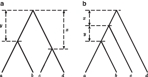
$$i = 1 , \ldots , 15$$\end{document}, as Ti when using it as a gene tree, and as Si when using it as a species tree. Similarly to the case of trees with three leaves, it is sufficient for us to consider only one labeling for each unlabeled species tree topology. We assume that the species tree is either (S1, λ) = ((a, b): y, (c, d): x) or (S4, λ) = (((a, b): y, c): x, d), where x and y are the positive lengths in coalescent time units of the two internal branches (Fig. 2).
Symmetric (a) and asymmetric (b) rooted, binary trees with leaf labels a, b, c, and d.
Probabilities and Deep Coalescence Costs for Reconciling Each of the 15 Rooted, Binary Gene Trees with Leaf Labels a, b, c, and d, Given Either the Species Tree (S1, λ) = ((a, b): y, (c, d): x) or (S4, λ) = (((a, b): y, c): x, d)
Our investigation of the consistency of the MDC criterion for symmetric and asymmetric species trees (S1, λ) and (S4, λ) makes use of the rearrangement inequality, which states that given two sequences of real numbers
\documentclass{aastex}
\usepackage{amsbsy}
\usepackage{amsfonts}
\usepackage{amssymb}
\usepackage{bm}
\usepackage{mathrsfs}
\usepackage{pifont}
\usepackage{stmaryrd}
\usepackage{textcomp}
\usepackage{portland, xspace}
\usepackage{amsmath, amsxtra}
\pagestyle{empty}
\DeclareMathSizes {10} {9} {7} {6}
\begin{document}
$$a_1 \leq \cdots \leq a_n$$\end{document} and
\documentclass{aastex}
\usepackage{amsbsy}
\usepackage{amsfonts}
\usepackage{amssymb}
\usepackage{bm}
\usepackage{mathrsfs}
\usepackage{pifont}
\usepackage{stmaryrd}
\usepackage{textcomp}
\usepackage{portland, xspace}
\usepackage{amsmath, amsxtra}
\pagestyle{empty}
\DeclareMathSizes {10} {9} {7} {6}
\begin{document}
$$b_1 \geq \cdots \geq b_n$$\end{document}, the inequality
\documentclass{aastex}
\usepackage{amsbsy}
\usepackage{amsfonts}
\usepackage{amssymb}
\usepackage{bm}
\usepackage{mathrsfs}
\usepackage{pifont}
\usepackage{stmaryrd}
\usepackage{textcomp}
\usepackage{portland, xspace}
\usepackage{amsmath, amsxtra}
\pagestyle{empty}
\DeclareMathSizes {10} {9} {7} {6}
\begin{document}
\begin{align*}
a_1b_1 + \cdots + a_nb_n \leq a_{ \pi ( 1 ) }b_1 + \cdots + a_{ \pi ( n ) }b_n \tag{3.2}
\end{align*}
\end{document}
holds for any permutation π of
\documentclass{aastex}
\usepackage{amsbsy}
\usepackage{amsfonts}
\usepackage{amssymb}
\usepackage{bm}
\usepackage{mathrsfs}
\usepackage{pifont}
\usepackage{stmaryrd}
\usepackage{textcomp}
\usepackage{portland, xspace}
\usepackage{amsmath, amsxtra}
\pagestyle{empty}
\DeclareMathSizes {10} {9} {7} {6}
\begin{document}
$$\{ 1 , \ldots , n \} $$\end{document} (Hardy et al., 1934). Note that if a1 is strictly smaller than each of
\documentclass{aastex}
\usepackage{amsbsy}
\usepackage{amsfonts}
\usepackage{amssymb}
\usepackage{bm}
\usepackage{mathrsfs}
\usepackage{pifont}
\usepackage{stmaryrd}
\usepackage{textcomp}
\usepackage{portland, xspace}
\usepackage{amsmath, amsxtra}
\pagestyle{empty}
\DeclareMathSizes {10} {9} {7} {6}
\begin{document}
$$a_2 , \ldots , a_n$$\end{document} and b1 is strictly greater than each of
\documentclass{aastex}
\usepackage{amsbsy}
\usepackage{amsfonts}
\usepackage{amssymb}
\usepackage{bm}
\usepackage{mathrsfs}
\usepackage{pifont}
\usepackage{stmaryrd}
\usepackage{textcomp}
\usepackage{portland, xspace}
\usepackage{amsmath, amsxtra}
\pagestyle{empty}
\DeclareMathSizes {10} {9} {7} {6}
\begin{document}
$$b_2 , \ldots , b_n$$\end{document}, then for any permutation π such that the equality in Eq. (3.2) holds, it is necessary that π(1) = 1 (and so a1 = aπ(1)). For otherwise, let π(1) = i > 1, and let π(j) = 1 for some j > 1. Because a1 < ai and b1 > bj, (a1b1 + aibj) − (aib1 + a1bj) = (a1 − ai)(b1 − bj) < 0. But this leads to a contradiction because the permutation π′ in which π′(1) = 1, π′(j) = i, and π′(k) = π(k) for k ≠ 1 and k ≠ j produces a sum
\documentclass{aastex}
\usepackage{amsbsy}
\usepackage{amsfonts}
\usepackage{amssymb}
\usepackage{bm}
\usepackage{mathrsfs}
\usepackage{pifont}
\usepackage{stmaryrd}
\usepackage{textcomp}
\usepackage{portland, xspace}
\usepackage{amsmath, amsxtra}
\pagestyle{empty}
\DeclareMathSizes {10} {9} {7} {6}
\begin{document}
$$\sum_{k = 1}^{n} a_{ \pi^{ \prime} ( k ) }b_k$$\end{document} strictly smaller than the smallest sum
\documentclass{aastex}
\usepackage{amsbsy}
\usepackage{amsfonts}
\usepackage{amssymb}
\usepackage{bm}
\usepackage{mathrsfs}
\usepackage{pifont}
\usepackage{stmaryrd}
\usepackage{textcomp}
\usepackage{portland, xspace}
\usepackage{amsmath, amsxtra}
\pagestyle{empty}
\DeclareMathSizes {10} {9} {7} {6}
\begin{document}
$$\sum_{k = 1}^{n}a_kb_k$$\end{document}.
In the proof below, the rearrangement inequality is applied to the list of probabilities (considered as {bi}) and the list of deep coalescence costs (considered as {ai}) of the 15 gene trees. As observed in Section 2.2, if two species tree candidates S and S′ have the same unlabeled topology, then
\documentclass{aastex}
\usepackage{amsbsy}
\usepackage{amsfonts}
\usepackage{amssymb}
\usepackage{bm}
\usepackage{mathrsfs}
\usepackage{pifont}
\usepackage{stmaryrd}
\usepackage{textcomp}
\usepackage{portland, xspace}
\usepackage{amsmath, amsxtra}
\pagestyle{empty}
\DeclareMathSizes {10} {9} {7} {6}
\begin{document}
$$\{ \alpha ( T , S ) \mid T \in R_1 \} = \{ \alpha ( T , S^{ \prime} ) \mid T \in R_1 \} $$\end{document} and
\documentclass{aastex}
\usepackage{amsbsy}
\usepackage{amsfonts}
\usepackage{amssymb}
\usepackage{bm}
\usepackage{mathrsfs}
\usepackage{pifont}
\usepackage{stmaryrd}
\usepackage{textcomp}
\usepackage{portland, xspace}
\usepackage{amsmath, amsxtra}
\pagestyle{empty}
\DeclareMathSizes {10} {9} {7} {6}
\begin{document}
$$\{ \alpha ( T , S ) \mid T \in R_2 \} = \{ \alpha ( T , S^{ \prime} ) \mid T \in R_2 \} $$\end{document}. Therefore, the rearrangement inequality can be applied separately in R1 and R2 to the probabilities and deep coalescence costs of gene trees.
3.2.1. Symmetric species trees
Given that the true species tree is (S1, λ), the probabilities of the 15 gene trees were computed by Rosenberg (2002), and they are reproduced in the second column of Table 1. The deep coalescence costs for reconciling each of the 15 gene trees within S1 are also given in Table 1. It can be observed from the table that Pr(T2 | S1, λ) = Pr(T3 | S1, λ), Pr(T4 | S1, λ) = Pr(T5 | S1, λ), Pr(T6 | S1, λ) = Pr(T7 | S1, λ), and
\documentclass{aastex}
\usepackage{amsbsy}
\usepackage{amsfonts}
\usepackage{amssymb}
\usepackage{bm}
\usepackage{mathrsfs}
\usepackage{pifont}
\usepackage{stmaryrd}
\usepackage{textcomp}
\usepackage{portland, xspace}
\usepackage{amsmath, amsxtra}
\pagestyle{empty}
\DeclareMathSizes {10} {9} {7} {6}
\begin{document}
$$\Pr ( T_8 \mid S_1 , { \bf \lambda} ) = \cdots = \Pr ( T_{15} \mid S_1 , { \bf \lambda} )$$\end{document}. Plugging the probability values and deep coalescence costs into Eq. (3.1), we have
\documentclass{aastex}
\usepackage{amsbsy}
\usepackage{amsfonts}
\usepackage{amssymb}
\usepackage{bm}
\usepackage{mathrsfs}
\usepackage{pifont}
\usepackage{stmaryrd}
\usepackage{textcomp}
\usepackage{portland, xspace}
\usepackage{amsmath, amsxtra}
\pagestyle{empty}
\DeclareMathSizes {10} {9} {7} {6}
\begin{document}
\begin{align*}
\overline{\alpha}_{S_1 , {\lambda}} (S_1) & = \sum_{i = 1}^{15}
\Pr (T_i \mid S_1 , {\lambda}) \alpha (T_i , S_1)
\\ & = \sum_{i = 1}^3 \Pr (T_i \mid S_1 , {\lambda} ) \alpha
(T_i , S_1) + \sum_{i = 4}^{15} \Pr (T_i \mid S_1 , {\lambda})
\alpha (T_i , S_1) \tag{3.3}
\end{align*}
\end{document}
\documentclass{aastex}
\usepackage{amsbsy}
\usepackage{amsfonts}
\usepackage{amssymb}
\usepackage{bm}
\usepackage{mathrsfs}
\usepackage{pifont}
\usepackage{stmaryrd}
\usepackage{textcomp}
\usepackage{portland, xspace}
\usepackage{amsmath, amsxtra}
\pagestyle{empty}
\DeclareMathSizes {10} {9} {7} {6}
\begin{document}
\begin{align*}
= 4 \Pr ( T_2 \mid S_1 , {\lambda}) + 2 \Pr (T_4 \mid S_1 ,
{\lambda}) + 2 \Pr (T_6 \mid S_1 , {\lambda}) + 16 \Pr (T_8 \mid
S_1 , {\lambda}) \quad \tag{3.4}
\end{align*}
\end{document}
Let S′ be a species tree candidate different from S1. We aim to prove that
\documentclass{aastex}
\usepackage{amsbsy}
\usepackage{amsfonts}
\usepackage{amssymb}
\usepackage{bm}
\usepackage{mathrsfs}
\usepackage{pifont}
\usepackage{stmaryrd}
\usepackage{textcomp}
\usepackage{portland, xspace}
\usepackage{amsmath, amsxtra}
\pagestyle{empty}
\DeclareMathSizes {10} {9} {7} {6}
\begin{document}
$$\overline{ \alpha}_{S_1 , { \bf \lambda}} ( S_1 ) < \overline{ \alpha}_{S_1 , { \bf \lambda}}( S^{ \prime} )$$\end{document}. There are two subcases to consider: S′ is symmetric, and S′ is asymmetric.
TreeS′ is symmetric. For gene trees in R1, it can be seen seen from Table 1 that Pr(T1 | S1, λ) > Pr(T2 | S1, λ) = Pr(T3 | S1, λ). In fact, Pr(T1 | S1, λ) is the largest probability among the 15 probability values
\documentclass{aastex}
\usepackage{amsbsy}
\usepackage{amsfonts}
\usepackage{amssymb}
\usepackage{bm}
\usepackage{mathrsfs}
\usepackage{pifont}
\usepackage{stmaryrd}
\usepackage{textcomp}
\usepackage{portland, xspace}
\usepackage{amsmath, amsxtra}
\pagestyle{empty}
\DeclareMathSizes {10} {9} {7} {6}
\begin{document}
$$\Pr ( T_1 \mid S_1 , { \bf \lambda} ) , \ldots , \Pr ( T_{15} \mid S_1 , { \bf \lambda} )$$\end{document}, so that the democratic vote method is consistent for symmetric species trees with four leaves (Degnan and Rosenberg, 2006). We also have α(T1, S1) = 0 < α(T2, S1) = α(T3, S1) = 2. Moreover, because S1 and S′ have the same unlabeled topology, the list {α(Ti, S′), i = 1, 2, 3} is a permutation of {α(Ti, S1), i = 1, 2, 3}. Applying the rearrangement inequality to the lists {α(Ti, S1), i = 1, 2, 3} and {Pr(Ti | S1, λ), i = 1, 2, 3}, we have
\documentclass{aastex}
\usepackage{amsbsy}
\usepackage{amsfonts}
\usepackage{amssymb}
\usepackage{bm}
\usepackage{mathrsfs}
\usepackage{pifont}
\usepackage{stmaryrd}
\usepackage{textcomp}
\usepackage{portland, xspace}
\usepackage{amsmath, amsxtra}
\pagestyle{empty}
\DeclareMathSizes {10} {9} {7} {6}
\begin{document}
\begin{align*}
\sum_{i = 1}^3 \Pr ( T_i \mid S_1 , { \boldsymbol \lambda} )
\alpha ( T_i , S_1 ) \leq \sum_{i = 1}^3 \Pr ( T_i \mid S_1 , {
\boldsymbol \lambda} ) \alpha ( T_i , S^{ \prime} ). \tag{3.5}
\end{align*}
\end{document}
For gene trees in R2, one can check from Table 1 that
\documentclass{aastex}
\usepackage{amsbsy}
\usepackage{amsfonts}
\usepackage{amssymb}
\usepackage{bm}
\usepackage{mathrsfs}
\usepackage{pifont}
\usepackage{stmaryrd}
\usepackage{textcomp}
\usepackage{portland, xspace}
\usepackage{amsmath, amsxtra}
\pagestyle{empty}
\DeclareMathSizes {10} {9} {7} {6}
\begin{document}
$$T_4 , \ldots , T_7$$\end{document} all have probabilities greater than those of
\documentclass{aastex}
\usepackage{amsbsy}
\usepackage{amsfonts}
\usepackage{amssymb}
\usepackage{bm}
\usepackage{mathrsfs}
\usepackage{pifont}
\usepackage{stmaryrd}
\usepackage{textcomp}
\usepackage{portland, xspace}
\usepackage{amsmath, amsxtra}
\pagestyle{empty}
\DeclareMathSizes {10} {9} {7} {6}
\begin{document}
$$T_8 , \ldots , T_{15}$$\end{document}, while their deep coalescence costs (for reconciling within S1) are smaller. Trees S1 and S′ have the same unlabeled topology, and hence the list
\documentclass{aastex}
\usepackage{amsbsy}
\usepackage{amsfonts}
\usepackage{amssymb}
\usepackage{bm}
\usepackage{mathrsfs}
\usepackage{pifont}
\usepackage{stmaryrd}
\usepackage{textcomp}
\usepackage{portland, xspace}
\usepackage{amsmath, amsxtra}
\pagestyle{empty}
\DeclareMathSizes {10} {9} {7} {6}
\begin{document}
$$\{ \alpha ( T_i , S^{ \prime} ) , i = 4 , \ldots , 15 \} $$\end{document} is a permutation of
\documentclass{aastex}
\usepackage{amsbsy}
\usepackage{amsfonts}
\usepackage{amssymb}
\usepackage{bm}
\usepackage{mathrsfs}
\usepackage{pifont}
\usepackage{stmaryrd}
\usepackage{textcomp}
\usepackage{portland, xspace}
\usepackage{amsmath, amsxtra}
\pagestyle{empty}
\DeclareMathSizes {10} {9} {7} {6}
\begin{document}
$$\{ \alpha ( T_i , S ) , i = 4 , \ldots , 15 \} $$\end{document}. We again apply the rearrangement inequality to the lists
\documentclass{aastex}
\usepackage{amsbsy}
\usepackage{amsfonts}
\usepackage{amssymb}
\usepackage{bm}
\usepackage{mathrsfs}
\usepackage{pifont}
\usepackage{stmaryrd}
\usepackage{textcomp}
\usepackage{portland, xspace}
\usepackage{amsmath, amsxtra}
\pagestyle{empty}
\DeclareMathSizes {10} {9} {7} {6}
\begin{document}
$$\{ \alpha ( T_i , S_1 ) , i = 4 , \ldots , 15 \} $$\end{document} and
\documentclass{aastex}
\usepackage{amsbsy}
\usepackage{amsfonts}
\usepackage{amssymb}
\usepackage{bm}
\usepackage{mathrsfs}
\usepackage{pifont}
\usepackage{stmaryrd}
\usepackage{textcomp}
\usepackage{portland, xspace}
\usepackage{amsmath, amsxtra}
\pagestyle{empty}
\DeclareMathSizes {10} {9} {7} {6}
\begin{document}
$$\{ \Pr ( T_i \mid S_1 , { \bf \lambda} ) , i = 4 , \ldots , 15 \} $$\end{document}, obtaining
\documentclass{aastex}
\usepackage{amsbsy}
\usepackage{amsfonts}
\usepackage{amssymb}
\usepackage{bm}
\usepackage{mathrsfs}
\usepackage{pifont}
\usepackage{stmaryrd}
\usepackage{textcomp}
\usepackage{portland, xspace}
\usepackage{amsmath, amsxtra}
\pagestyle{empty}
\DeclareMathSizes {10} {9} {7} {6}
\begin{document}
\begin{align*}
\sum_{i = 4}^{15} \Pr ( T_i \mid S_1 , { \boldsymbol \lambda} )
\alpha ( T_i , S_1 ) \leq \sum_{i = 4}^{15} \Pr ( T_i \mid S_1 , {
\boldsymbol \lambda} ) \alpha ( T_i , S^{ \prime} ). \tag{3.6}
\end{align*}
\end{document}
From Eqs. (3.3), (3.5), and (3.6), we have
\documentclass{aastex}
\usepackage{amsbsy}
\usepackage{amsfonts}
\usepackage{amssymb}
\usepackage{bm}
\usepackage{mathrsfs}
\usepackage{pifont}
\usepackage{stmaryrd}
\usepackage{textcomp}
\usepackage{portland, xspace}
\usepackage{amsmath, amsxtra}
\pagestyle{empty}
\DeclareMathSizes {10} {9} {7} {6}
\begin{document}
$$\overline{ \alpha}_{S_1 , { \bf \lambda}} ( S_1 ) \leq \overline{ \alpha}_{S_1 , { \bf \lambda}} ( S^{ \prime} )$$\end{document}. Further, if
\documentclass{aastex}
\usepackage{amsbsy}
\usepackage{amsfonts}
\usepackage{amssymb}
\usepackage{bm}
\usepackage{mathrsfs}
\usepackage{pifont}
\usepackage{stmaryrd}
\usepackage{textcomp}
\usepackage{portland, xspace}
\usepackage{amsmath, amsxtra}
\pagestyle{empty}
\DeclareMathSizes {10} {9} {7} {6}
\begin{document}
$$\overline{ \alpha}_{S_1 , { \bf \lambda}} ( S_1 ) = \overline{ \alpha}_{S_1 , { \bf \lambda}} ( S^{ \prime} )$$\end{document}, then it is necessary that the equality in Eq. (3.5) holds. However, Pr(T1 | S1, λ) is strictly greater than Pr(T2 | S1, λ) and Pr(T3 | S1, λ), while α(T1, S1) is strictly smaller than α(T2, S1) and α(T3, S1). Using the equality condition in the rearrangement inequality, the equality in Eq. (3.5) holds only when α(T1, S′) = α(T1, S1) = 0, which is true only if S′ = S1. Therefore,
\documentclass{aastex}
\usepackage{amsbsy}
\usepackage{amsfonts}
\usepackage{amssymb}
\usepackage{bm}
\usepackage{mathrsfs}
\usepackage{pifont}
\usepackage{stmaryrd}
\usepackage{textcomp}
\usepackage{portland, xspace}
\usepackage{amsmath, amsxtra}
\pagestyle{empty}
\DeclareMathSizes {10} {9} {7} {6}
\begin{document}
$$\overline{ \alpha}_{S_1 , { \bf \lambda}} ( S_1 ) < \overline{ \alpha}_{S_1 , { \bf \lambda}} ( S^{ \prime} )$$\end{document} for any symmetric species tree candidate S′ ≠ S1.
TreeS′ is asymmetric. In this case, S′ and S4 have the same unlabeled topology, and so the lists {α(Ti, S′), i = 1, 2, 3} and
\documentclass{aastex}
\usepackage{amsbsy}
\usepackage{amsfonts}
\usepackage{amssymb}
\usepackage{bm}
\usepackage{mathrsfs}
\usepackage{pifont}
\usepackage{stmaryrd}
\usepackage{textcomp}
\usepackage{portland, xspace}
\usepackage{amsmath, amsxtra}
\pagestyle{empty}
\DeclareMathSizes {10} {9} {7} {6}
\begin{document}
$$\{ \alpha ( T_i , S^{ \prime} ) , i = 4 , \ldots , 15 \} $$\end{document} are permutations of {α(Ti, S4), i = 1, 2, 3} and
\documentclass{aastex}
\usepackage{amsbsy}
\usepackage{amsfonts}
\usepackage{amssymb}
\usepackage{bm}
\usepackage{mathrsfs}
\usepackage{pifont}
\usepackage{stmaryrd}
\usepackage{textcomp}
\usepackage{portland, xspace}
\usepackage{amsmath, amsxtra}
\pagestyle{empty}
\DeclareMathSizes {10} {9} {7} {6}
\begin{document}
$$\{ \alpha ( T_i , S_4 ) , i = 4 , \ldots , 15 \} $$\end{document}, respectively. From Table 1, notice that α(T1, S4) = 1 < α(T2, S4) = α(T3, S4) = 2. Applying the rearrangement inequality to the lists {α(Ti, S4), i = 1, 2, 3} and {Pr(Ti | S1, λ), i = 1, 2, 3}, we have
\documentclass{aastex}
\usepackage{amsbsy}
\usepackage{amsfonts}
\usepackage{amssymb}
\usepackage{bm}
\usepackage{mathrsfs}
\usepackage{pifont}
\usepackage{stmaryrd}
\usepackage{textcomp}
\usepackage{portland, xspace}
\usepackage{amsmath, amsxtra}
\pagestyle{empty}
\DeclareMathSizes {10} {9} {7} {6}
\begin{document}
\begin{align*}
\sum_{i = 1}^3 \Pr ( T_i \mid S_1 , { \boldsymbol \lambda} )
\alpha ( T_i , S^{ \prime} ) \geq \Pr ( T_1 \mid S_1 , {
\boldsymbol \lambda} ) + 4 \Pr ( T_2 \mid S_1 , { \boldsymbol
\lambda} ). \tag{3.7}
\end{align*}
\end{document}
For gene trees in R2, the four smallest values among
\documentclass{aastex}
\usepackage{amsbsy}
\usepackage{amsfonts}
\usepackage{amssymb}
\usepackage{bm}
\usepackage{mathrsfs}
\usepackage{pifont}
\usepackage{stmaryrd}
\usepackage{textcomp}
\usepackage{portland, xspace}
\usepackage{amsmath, amsxtra}
\pagestyle{empty}
\DeclareMathSizes {10} {9} {7} {6}
\begin{document}
$$\alpha ( T_4 , S_4 ) , \ldots , \alpha ( T_{15} , S_4 )$$\end{document} are smaller than or equal to 1, while the remaining eight values are at least 2. We have also noticed above that
\documentclass{aastex}
\usepackage{amsbsy}
\usepackage{amsfonts}
\usepackage{amssymb}
\usepackage{bm}
\usepackage{mathrsfs}
\usepackage{pifont}
\usepackage{stmaryrd}
\usepackage{textcomp}
\usepackage{portland, xspace}
\usepackage{amsmath, amsxtra}
\pagestyle{empty}
\DeclareMathSizes {10} {9} {7} {6}
\begin{document}
$$T_4 , \ldots , T_7$$\end{document} all have probabilities greater than the probabilities of
\documentclass{aastex}
\usepackage{amsbsy}
\usepackage{amsfonts}
\usepackage{amssymb}
\usepackage{bm}
\usepackage{mathrsfs}
\usepackage{pifont}
\usepackage{stmaryrd}
\usepackage{textcomp}
\usepackage{portland, xspace}
\usepackage{amsmath, amsxtra}
\pagestyle{empty}
\DeclareMathSizes {10} {9} {7} {6}
\begin{document}
$$T_8 , \ldots , T_{15}$$\end{document}. However, the relative order between Pr(T4 | S1, λ) = Pr(T5 | S1, λ) and Pr(T6 | S1, λ) = Pr(T7 | S1, λ) depends on the branch lengths x and y. Assuming that Pr(T4 | S1, λ) ≥ Pr(T6 | S1, λ), then
\documentclass{aastex}
\usepackage{amsbsy}
\usepackage{amsfonts}
\usepackage{amssymb}
\usepackage{bm}
\usepackage{mathrsfs}
\usepackage{pifont}
\usepackage{stmaryrd}
\usepackage{textcomp}
\usepackage{portland, xspace}
\usepackage{amsmath, amsxtra}
\pagestyle{empty}
\DeclareMathSizes {10} {9} {7} {6}
\begin{document}
\begin{align*}
\sum_{i = 4}^{15} \Pr ( T_i \mid S_1 , { \boldsymbol \lambda} )
\alpha ( T_i , S^{ \prime} ) \geq \Pr ( T_4 \mid S_1 , {
\boldsymbol \lambda} ) + 2 \Pr ( T_6 \mid S_1 , { \boldsymbol
\lambda} ) + 22 \Pr ( T_8 \mid S_1 , { \boldsymbol \lambda} ) ,
\tag{3.8}
\end{align*}\end{document}
It is straightforward to check that Eq. (3.9) and (3.10) are always greater than zero for all positive x and y. Consequently,
\documentclass{aastex}
\usepackage{amsbsy}
\usepackage{amsfonts}
\usepackage{amssymb}
\usepackage{bm}
\usepackage{mathrsfs}
\usepackage{pifont}
\usepackage{stmaryrd}
\usepackage{textcomp}
\usepackage{portland, xspace}
\usepackage{amsmath, amsxtra}
\pagestyle{empty}
\DeclareMathSizes {10} {9} {7} {6}
\begin{document}
$$\overline{ \alpha}_{S_1 , { \bf \lambda}} ( S_1 ) < \overline{ \alpha}_{S_1 , { \bf \lambda}} ( S^{ \prime} )$$
\end{document} for all asymmetric S′.
Whether the species tree candidate S′ is asymmetric or symmetric, if S′ ≠ S1, then
\documentclass{aastex}
\usepackage{amsbsy}
\usepackage{amsfonts}
\usepackage{amssymb}
\usepackage{bm}
\usepackage{mathrsfs}
\usepackage{pifont}
\usepackage{stmaryrd}
\usepackage{textcomp}
\usepackage{portland, xspace}
\usepackage{amsmath, amsxtra}
\pagestyle{empty}
\DeclareMathSizes {10} {9} {7} {6}
\begin{document}
$$\overline{ \alpha}_{S_1 , { \bf \lambda}} ( S_1 ) < \overline{ \alpha}_{S_1 , { \bf \lambda}} ( S^{ \prime} )$$
\end{document}. Therefore, in the case of four-taxon, symmetric species trees, the unique asymptotic MDC tree matches the species tree topology. The MDC criterion is statistically consistent in this case.
3.2.2. Asymmetric species trees
Our treatment for the case of the asymmetric species tree (S4, λ) = (((a, b): y, c): x, d) is similar to the treatment for the symmetric species tree S1 in Section 3.2.1. The probabilities of the 15 gene trees
\documentclass{aastex}
\usepackage{amsbsy}
\usepackage{amsfonts}
\usepackage{amssymb}
\usepackage{bm}
\usepackage{mathrsfs}
\usepackage{pifont}
\usepackage{stmaryrd}
\usepackage{textcomp}
\usepackage{portland, xspace}
\usepackage{amsmath, amsxtra}
\pagestyle{empty}
\DeclareMathSizes {10} {9} {7} {6}
\begin{document}
$$T_1 , \ldots , T_{15}$$
\end{document} given the species tree S4, computed by Rosenberg (2002), are reproduced in the fourth column of Table 1. Again, there are two subcases to consider, depending on whether the species tree candidate S′ is asymmetric or symmetric.
TreeS′ is asymmetric. For gene trees in R1, Pr(T1 | S4, λ) > Pr(T2 | S4, λ) = Pr(T3 | S4, λ), while α(T1, S4) = 1 < α(T2, S4) = α(T3, S4) = 2. Also, because S′ and S4 have the same unlabeled tree topology, the list {α(Ti, S′), i = 1, 2, 3} is a permutation of {α(Ti, S4), i = 1, 2, 3}. By using the rearrangement inequality, we have
\documentclass{aastex}
\usepackage{amsbsy}
\usepackage{amsfonts}
\usepackage{amssymb}
\usepackage{bm}
\usepackage{mathrsfs}
\usepackage{pifont}
\usepackage{stmaryrd}
\usepackage{textcomp}
\usepackage{portland, xspace}
\usepackage{amsmath, amsxtra}
\pagestyle{empty}
\DeclareMathSizes {10} {9} {7} {6}
\begin{document}
\begin{align*}
\sum_{i = 1}^3 \Pr ( T_i \mid S_4 , { \boldsymbol \lambda} )
\alpha ( T_i , S_4 ) \leq \sum_{i = 1}^3 \Pr ( T_i \mid S_4 , {
\boldsymbol \lambda} ) \alpha ( T_i , S^{ \prime} ). \tag{3.11}
\end{align*}
\end{document}
For gene trees in R2, we make three observations about their probabilities:
However, ey > 1 for positive y, while the left hand side is always smaller than 1 because
\documentclass{aastex}
\usepackage{amsbsy}
\usepackage{amsfonts}
\usepackage{amssymb}
\usepackage{bm}
\usepackage{mathrsfs}
\usepackage{pifont}
\usepackage{stmaryrd}
\usepackage{textcomp}
\usepackage{portland, xspace}
\usepackage{amsmath, amsxtra}
\pagestyle{empty}
\DeclareMathSizes {10} {9} {7} {6}
\begin{document}
\begin{align*}
\frac { 2 } { 3 } - \frac { 1 } { 2 } e^ { - x } - \frac { 1 } { 6 } e^ { - 3x } - ( 1 - e^ { - x } ) = - \frac { ( e^ { - x } - 1 ) ^2 ( e^ { - x } + 2 ) } { 6 } ,
\end{align*}
\end{document}
which is smaller than zero for all positive x. We note that although the relative order of Pr(T5 | S4, λ) and Pr(T8 | S4, λ) depends on x and y, this is not important as the deep coalescence costs for reconciling either T5 or T8 within S4 have the same value, 1.
As for the deep coalescence costs of gene trees in R2, α(T4, S4) = 0 < α(T5, S4) = α(T8, S4) = α(T9, S4) = 1 < α(T12, S4) = α(T13, S4) = 2, while for each of the remaining six trees, the cost is 3. Based on the relative orders of the probabilities Pr(Ti | S4, λ) and deep coalescence costs α(Ti, S4), by using the rearrangement inequality, we have
\documentclass{aastex}
\usepackage{amsbsy}
\usepackage{amsfonts}
\usepackage{amssymb}
\usepackage{bm}
\usepackage{mathrsfs}
\usepackage{pifont}
\usepackage{stmaryrd}
\usepackage{textcomp}
\usepackage{portland, xspace}
\usepackage{amsmath, amsxtra}
\pagestyle{empty}
\DeclareMathSizes {10} {9} {7} {6}
\begin{document}
\begin{align*}
\sum_{i = 4}^{15} \Pr ( T_i \mid S_4 , { \boldsymbol \lambda} )
\alpha ( T_i , S_4 ) \leq \sum_{i = 4}^{15} \Pr ( T_i \mid S_4 , {
\boldsymbol \lambda} ) \alpha ( T_i , S^{ \prime} ). \tag{3.12}
\end{align*}\end{document}
Equations (3.11) and (3.12) imply that
\documentclass{aastex}
\usepackage{amsbsy}
\usepackage{amsfonts}
\usepackage{amssymb}
\usepackage{bm}
\usepackage{mathrsfs}
\usepackage{pifont}
\usepackage{stmaryrd}
\usepackage{textcomp}
\usepackage{portland, xspace}
\usepackage{amsmath, amsxtra}
\pagestyle{empty}
\DeclareMathSizes {10} {9} {7} {6}
\begin{document}
$$\overline{ \alpha}_{S_4 , { \bf \lambda}} ( S_4 ) \leq \overline{ \alpha}_{S_4 , { \bf \lambda}} ( S^{ \prime} )$$\end{document} for any asymmetric species tree candidate S′. If
\documentclass{aastex}
\usepackage{amsbsy}
\usepackage{amsfonts}
\usepackage{amssymb}
\usepackage{bm}
\usepackage{mathrsfs}
\usepackage{pifont}
\usepackage{stmaryrd}
\usepackage{textcomp}
\usepackage{portland, xspace}
\usepackage{amsmath, amsxtra}
\pagestyle{empty}
\DeclareMathSizes {10} {9} {7} {6}
\begin{document}
$$\overline{ \alpha}_{S_4 , { \bf \lambda}} ( S_4 ) = \overline{ \alpha}_{S_4 , { \bf \lambda}} ( S^{ \prime} )$$
\end{document}, then equality must hold in Eq. (3.12). Because Pr(T4 | S4, λ) is strictly greater than the probabilities of other gene trees in R2, while α(T4, S4) is strictly smaller than their deep coalescence costs, the equality in Eq. (3.12) holds only when α(T4, S′) = α(T4, S4) = 0, which in turn holds only when S′ = S4. Therefore, for any asymmetric species tree candidate
\documentclass{aastex}
\usepackage{amsbsy}
\usepackage{amsfonts}
\usepackage{amssymb}
\usepackage{bm}
\usepackage{mathrsfs}
\usepackage{pifont}
\usepackage{stmaryrd}
\usepackage{textcomp}
\usepackage{portland, xspace}
\usepackage{amsmath, amsxtra}
\pagestyle{empty}
\DeclareMathSizes {10} {9} {7} {6}
\begin{document}
$$S^\prime \neq S_4 , \overline{ \alpha}_{S_4 , { \bf \lambda}} ( S_4 ) < \overline{ \alpha}_{S_4 , { \bf \lambda}} ( S^{ \prime} )$$\end{document}.
TreeS′ is symmetric. There are three symmetric species tree candidates—S1, S2, and S3—and we consider each one of them in turn:
Because we assume species tree branch lengths are positive, in order for a positive value of y to satisfy Eq. (3.13) or Eq. (3.14), the right hand sides of Eq. (3.13) and Eq. (3.14) must be positive. Both of these requirements yield the same condition:
\documentclass{aastex}
\usepackage{amsbsy}
\usepackage{amsfonts}
\usepackage{amssymb}
\usepackage{bm}
\usepackage{mathrsfs}
\usepackage{pifont}
\usepackage{stmaryrd}
\usepackage{textcomp}
\usepackage{portland, xspace}
\usepackage{amsmath, amsxtra}
\pagestyle{empty}
\DeclareMathSizes {10} {9} {7} {6}
\begin{document}
\begin{align*}
18e^{3x} - 21e^{2x} - 4 < 0. \tag{3.15}
\end{align*}
\end{document}
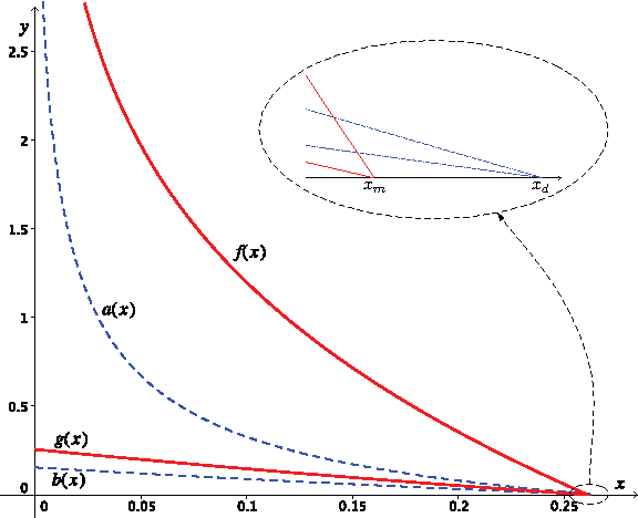
In addition, it is straightforward to verify that when Eq. (3.15) holds, f (x) > g(x).
Figure 3 shows the plots of f (x) and g(x). To the right of the curve f (x) in the figure, neither Eq. (3.13) nor Eq. (3.14) is satisfied, and the species tree S4 is the asymptotic MDC tree. To the left of this curve, Eq. (3.13) holds, implying that αS4,λ(S4) is not the smallest, and therefore, S4 cannot be the asymptotic MDC tree. More precisely,
If 0 ≤ f (x) < y or if x is greater than or equal to the root xm ≈ 0.2612 of Eq. (3.15), then the asymptotic MDC tree is the species tree S4;
If 0 ≤ g(x) < y < f (x), then S1 is the only species tree candidate that has expected deep coalescence cost smaller than that of S4;
If 0 < y ≤ g(x), then the trees S1, S2, and S3 all have expected deep coalescence cost smaller than that of S4.
Anomaly zones of the minimizing-deep-coalescence (MDC) criterion for asymmetric species trees with four leaves. In the region bounded by y = g(x) and the two axes, there are three candidate species trees with lower expected deep coalescence costs than the true species tree, while in the region bounded by the y-axis, y = g(x) and y = f(x), there is one such anomalous candidate species tree. In this figure, the anomaly zones of the democratic vote method, defined by a(x) and b(x), are shown in dashed lines. The definitions of branch lengths x and y appear in Figure 2b.
We also note that in the boundary case where y = f (x) > 0, both S1 and S4 have the same expected deep coalescence cost. In the limit in which the number of gene trees goes to infinity, the MDC criterion considers S1 and S4 equally good, and so we also say that the MDC criterion is not statistically consistent in this case.
Because f (x) approaches infinity as x approaches zero, for any given y, we can always make x small enough so that Eq. (3.13) holds. In other words, we can set x sufficiently small so that the species tree S4 is not the asymptotic MDC tree. In addition, when y < g(0) ≈ 0.2559, we can always choose sufficiently small x so that Eq. (3.14) holds, giving all three species tree candidates S1, S2, and S3 smaller expected deep coalescence cost than the species tree S4. Thus, for very small x, the MDC criterion is very likely to infer an incorrect estimate of the true species tree. The effects of x and y on the MDC criterion are similar to their effects on the democratic vote method (Degnan and Rosenberg, 2006).
Figure 3 also plots the anomaly zones of the democratic vote method, defined by functions
\documentclass{aastex}
\usepackage{amsbsy}
\usepackage{amsfonts}
\usepackage{amssymb}
\usepackage{bm}
\usepackage{mathrsfs}
\usepackage{pifont}
\usepackage{stmaryrd}
\usepackage{textcomp}
\usepackage{portland, xspace}
\usepackage{amsmath, amsxtra}
\pagestyle{empty}
\DeclareMathSizes {10} {9} {7} {6}
\begin{document}
$$a ( x ) = \ln \Big( \frac { 2 } { 3 } + \frac { 3e^ { 2x } - 2 } { 18 ( e^ { 3x } - e^ { 2x } ) } \Big)$$
\end{document} and
\documentclass{aastex}
\usepackage{amsbsy}
\usepackage{amsfonts}
\usepackage{amssymb}
\usepackage{bm}
\usepackage{mathrsfs}
\usepackage{pifont}
\usepackage{stmaryrd}
\usepackage{textcomp}
\usepackage{portland, xspace}
\usepackage{amsmath, amsxtra}
\pagestyle{empty}
\DeclareMathSizes {10} {9} {7} {6}
\begin{document}
$$b ( x ) = \ln \Big( \frac { 2 } { 3 } + \frac { 5e^ { 2x } - 2 }
{ 6 ( 3e^ { 3x } - 2e^ { 2x } ) } \Big)$$
\end{document} (Degnan and Rosenberg, 2006). Similar to the MDC criterion, the space of branch lengths x and y is also divided into three regions. To the right of the curve a(x) in the figure, the democratic vote method is statistically consistent, that is, the most frequent gene tree has the same labeled topology as the species tree. In the region bounded by a(x) and b(x), there is exactly one labeled topology different from the species tree with higher probability than a matching gene tree. In the region below b(x), there are three anomalous gene tree topologies.
It is interesting to see that the anomaly zones of the MDC criterion are larger than those of the democratic vote method. The largest value such that the MDC criterion is inconsistent when both branch lengths have the same value is x = y ≈ 0.2215, whereas the corresponding length for the democratic vote is x = y ≈ 0.1569 (Degnan and Rosenberg, 2006). However, it is not the case that a(x) and b(x) are always smaller than f (x) and g(x) (Fig. 3). The functions a(x) and b(x) intersect with the x-axis at xd ≈ 0.2654, while f (x) = g(x) = 0 at xm ≈ 0.2612. In the region bounded by the x-axis and the curves f (x) and a(x), the MDC criterion is consistent, whereas the democratic vote method is not consistent.
Remarks. It is possible to obtain the consistency properties of the MDC criterion on trees with four leaves by an exhaustive approach, that is, by directly computing the expected deep coalescence cost for every species tree candidate and comparing it with the corresponding cost of the parametric species tree. However, our approach using the rearrangement inequality provides a more concise proof that gives us some insight into the anomaly zones of the MDC criterion. As we have shown, only asymmetric species trees can produce anomalous candidate trees, which are symmetric. Intuitively, both for true species trees that are symmetric and for those that are asymmetric, the probabilities and deep coalescence costs of gene trees in each of the sets R1 and R2 are monotonic, but in opposite order. Therefore, by the rearrangement inequality, a candidate species tree that has the same unlabeled topology as the true species tree cannot have a smaller expected deep coalescence cost. This reasoning explains why the true species tree and anomalous candidate species trees must have different unlabeled topologies.
3.3. Trees with five or more leaves
We prove in this section that for any species tree topology with at least five leaves, there always exists a set of branch lengths that makes the MDC criterion infer the incorrect species tree topology in the limit as the number of sampled gene trees goes to infinity. Our approach is to make certain branches long enough to force the species tree to behave like an asymmetric four-leaf tree. For a rooted, binary (species) tree with at least five leaves, the longest path from its root to one of its leaves must have length at least three, for otherwise it cannot have more than four leaves. Call this path the “main” path in the tree, and consider the remaining parts of the tree as four subtrees
\documentclass{aastex}
\usepackage{amsbsy}
\usepackage{amsfonts}
\usepackage{amssymb}
\usepackage{bm}
\usepackage{mathrsfs}
\usepackage{pifont}
\usepackage{stmaryrd}
\usepackage{textcomp}
\usepackage{portland, xspace}
\usepackage{amsmath, amsxtra}
\pagestyle{empty}
\DeclareMathSizes {10} {9} {7} {6}
\begin{document}
$$A_1 , \ldots , A_4$$
\end{document} attached to this path (Fig. 4). None of these subtrees can be empty, although one or more of these subtrees (but not all) can each be a single leaf. If all internal branches of these subtrees, along with the four branches labeled
\documentclass{aastex}
\usepackage{amsbsy}
\usepackage{amsfonts}
\usepackage{amssymb}
\usepackage{bm}
\usepackage{mathrsfs}
\usepackage{pifont}
\usepackage{stmaryrd}
\usepackage{textcomp}
\usepackage{portland, xspace}
\usepackage{amsmath, amsxtra}
\pagestyle{empty}
\DeclareMathSizes {10} {9} {7} {6}
\begin{document}
$$e_1 , \ldots , e_4$$
\end{document}, are arbitrarily long, then these subtrees can be “collapsed” into single leaves, resulting in an asymmetric four-leaf tree. Because we have already shown in Section 3.2.2 that such a species tree can mislead the MDC criterion, this reduction implies that the MDC criterion is also statistically inconsistent for trees with at least five leaves.
A tree with at least five leaves (left), illustrating the embedded structure of an asymmetric four-leaf tree (right). The path with length at least three between the root and some leaf is shown with a thick line. Each of the triangles, representing taxon groups, contains at least one leaf.
This argument can be made more rigorous as follows. If S has five or more leaves, then S has the same structure as the tree on the left in Figure 4, that is, S is obtained from S4 = (((a, b), c), d) by substituting leaves a, b, c, and d with nonempty subtrees
\documentclass{aastex}
\usepackage{amsbsy}
\usepackage{amsfonts}
\usepackage{amssymb}
\usepackage{bm}
\usepackage{mathrsfs}
\usepackage{pifont}
\usepackage{stmaryrd}
\usepackage{textcomp}
\usepackage{portland, xspace}
\usepackage{amsmath, amsxtra}
\pagestyle{empty}
\DeclareMathSizes {10} {9} {7} {6}
\begin{document}
$$A_1 , \ldots , A_4$$
\end{document}, respectively. For each
\documentclass{aastex}
\usepackage{amsbsy}
\usepackage{amsfonts}
\usepackage{amssymb}
\usepackage{bm}
\usepackage{mathrsfs}
\usepackage{pifont}
\usepackage{stmaryrd}
\usepackage{textcomp}
\usepackage{portland, xspace}
\usepackage{amsmath, amsxtra}
\pagestyle{empty}
\DeclareMathSizes {10} {9} {7} {6}
\begin{document}
$$i = 1 , \ldots , 15$$\end{document}, let
\documentclass{aastex}
\usepackage{amsbsy}
\usepackage{amsfonts}
\usepackage{amssymb}
\usepackage{bm}
\usepackage{mathrsfs}
\usepackage{pifont}
\usepackage{stmaryrd}
\usepackage{textcomp}
\usepackage{portland, xspace}
\usepackage{amsmath, amsxtra}
\pagestyle{empty}
\DeclareMathSizes {10} {9} {7} {6}
\begin{document}
$$S_i^{ \prime} = T_i^{ \prime}$$\end{document} be the tree obtained from the corresponding Si = Ti in Table 1 using the same substitutions. Let hi be a valid coalescent history for reconciling the four-leaf gene tree Ti within S4. The coalescent history is a list of coalescence events along with a list of species tree internal branches (including the branch prior to the root of the species tree) on which they occur (Degnan and Salter, 2005; Rosenberg, 2007; Than et al., 2007). From hi, we create a coalescent history
\documentclass{aastex}
\usepackage{amsbsy}
\usepackage{amsfonts}
\usepackage{amssymb}
\usepackage{bm}
\usepackage{mathrsfs}
\usepackage{pifont}
\usepackage{stmaryrd}
\usepackage{textcomp}
\usepackage{portland, xspace}
\usepackage{amsmath, amsxtra}
\pagestyle{empty}
\DeclareMathSizes {10} {9} {7} {6}
\begin{document}
$$h_i^{ \prime}$$\end{document} for reconciling the gene tree
\documentclass{aastex}
\usepackage{amsbsy}
\usepackage{amsfonts}
\usepackage{amssymb}
\usepackage{bm}
\usepackage{mathrsfs}
\usepackage{pifont}
\usepackage{stmaryrd}
\usepackage{textcomp}
\usepackage{portland, xspace}
\usepackage{amsmath, amsxtra}
\pagestyle{empty}
\DeclareMathSizes {10} {9} {7} {6}
\begin{document}
$$T_i^{ \prime}$$\end{document} within S. We require that
\documentclass{aastex}
\usepackage{amsbsy}
\usepackage{amsfonts}
\usepackage{amssymb}
\usepackage{bm}
\usepackage{mathrsfs}
\usepackage{pifont}
\usepackage{stmaryrd}
\usepackage{textcomp}
\usepackage{portland, xspace}
\usepackage{amsmath, amsxtra}
\pagestyle{empty}
\DeclareMathSizes {10} {9} {7} {6}
\begin{document}
$$h_i^{ \prime}$$\end{document} satisfy the following two conditions:
In each internal branch of subtrees
\documentclass{aastex}
\usepackage{amsbsy}
\usepackage{amsfonts}
\usepackage{amssymb}
\usepackage{bm}
\usepackage{mathrsfs}
\usepackage{pifont}
\usepackage{stmaryrd}
\usepackage{textcomp}
\usepackage{portland, xspace}
\usepackage{amsmath, amsxtra}
\pagestyle{empty}
\DeclareMathSizes {10} {9} {7} {6}
\begin{document}
$$A_1 , \ldots , A_4$$\end{document}, as well as in each of the branches labeled
\documentclass{aastex}
\usepackage{amsbsy}
\usepackage{amsfonts}
\usepackage{amssymb}
\usepackage{bm}
\usepackage{mathrsfs}
\usepackage{pifont}
\usepackage{stmaryrd}
\usepackage{textcomp}
\usepackage{portland, xspace}
\usepackage{amsmath, amsxtra}
\pagestyle{empty}
\DeclareMathSizes {10} {9} {7} {6}
\begin{document}
$$e_1 , \ldots , e_4$$\end{document} in Figure 4, there is exactly one coalescence event. This implies that in each internal branch of
\documentclass{aastex}
\usepackage{amsbsy}
\usepackage{amsfonts}
\usepackage{amssymb}
\usepackage{bm}
\usepackage{mathrsfs}
\usepackage{pifont}
\usepackage{stmaryrd}
\usepackage{textcomp}
\usepackage{portland, xspace}
\usepackage{amsmath, amsxtra}
\pagestyle{empty}
\DeclareMathSizes {10} {9} {7} {6}
\begin{document}
$$A_1 , \ldots , A_4$$\end{document} and in each branch
\documentclass{aastex}
\usepackage{amsbsy}
\usepackage{amsfonts}
\usepackage{amssymb}
\usepackage{bm}
\usepackage{mathrsfs}
\usepackage{pifont}
\usepackage{stmaryrd}
\usepackage{textcomp}
\usepackage{portland, xspace}
\usepackage{amsmath, amsxtra}
\pagestyle{empty}
\DeclareMathSizes {10} {9} {7} {6}
\begin{document}
$$e_1 , \ldots , e_4$$\end{document}, exactly two gene lineages enter, and they coalesce into one lineage.
Denoting the single gene lineages in
\documentclass{aastex}
\usepackage{amsbsy}
\usepackage{amsfonts}
\usepackage{amssymb}
\usepackage{bm}
\usepackage{mathrsfs}
\usepackage{pifont}
\usepackage{stmaryrd}
\usepackage{textcomp}
\usepackage{portland, xspace}
\usepackage{amsmath, amsxtra}
\pagestyle{empty}
\DeclareMathSizes {10} {9} {7} {6}
\begin{document}
$$e_1 , \ldots , e_4$$\end{document} respectively as
\documentclass{aastex}
\usepackage{amsbsy}
\usepackage{amsfonts}
\usepackage{amssymb}
\usepackage{bm}
\usepackage{mathrsfs}
\usepackage{pifont}
\usepackage{stmaryrd}
\usepackage{textcomp}
\usepackage{portland, xspace}
\usepackage{amsmath, amsxtra}
\pagestyle{empty}
\DeclareMathSizes {10} {9} {7} {6}
\begin{document}
$$g_1 , \ldots , g_4$$\end{document}, we can think of them as gene lineages a, b, c, and d in S4. We now require that the lineages
\documentclass{aastex}
\usepackage{amsbsy}
\usepackage{amsfonts}
\usepackage{amssymb}
\usepackage{bm}
\usepackage{mathrsfs}
\usepackage{pifont}
\usepackage{stmaryrd}
\usepackage{textcomp}
\usepackage{portland, xspace}
\usepackage{amsmath, amsxtra}
\pagestyle{empty}
\DeclareMathSizes {10} {9} {7} {6}
\begin{document}
$$g_1 , \ldots , g_4$$\end{document} coalesce on the branches
\documentclass{aastex}
\usepackage{amsbsy}
\usepackage{amsfonts}
\usepackage{amssymb}
\usepackage{bm}
\usepackage{mathrsfs}
\usepackage{pifont}
\usepackage{stmaryrd}
\usepackage{textcomp}
\usepackage{portland, xspace}
\usepackage{amsmath, amsxtra}
\pagestyle{empty}
\DeclareMathSizes {10} {9} {7} {6}
\begin{document}
$$e_y^{ \prime}$$\end{document},
\documentclass{aastex}
\usepackage{amsbsy}
\usepackage{amsfonts}
\usepackage{amssymb}
\usepackage{bm}
\usepackage{mathrsfs}
\usepackage{pifont}
\usepackage{stmaryrd}
\usepackage{textcomp}
\usepackage{portland, xspace}
\usepackage{amsmath, amsxtra}
\pagestyle{empty}
\DeclareMathSizes {10} {9} {7} {6}
\begin{document}
$$e_x^{ \prime}$$\end{document}, and
\documentclass{aastex}
\usepackage{amsbsy}
\usepackage{amsfonts}
\usepackage{amssymb}
\usepackage{bm}
\usepackage{mathrsfs}
\usepackage{pifont}
\usepackage{stmaryrd}
\usepackage{textcomp}
\usepackage{portland, xspace}
\usepackage{amsmath, amsxtra}
\pagestyle{empty}
\DeclareMathSizes {10} {9} {7} {6}
\begin{document}
$$e_r^{ \prime}$$\end{document} of the species tree S in the same pattern as a, b, c, and d coalesce on the branches ey, ex, and er of S4. Here, we attach the branches
\documentclass{aastex}
\usepackage{amsbsy}
\usepackage{amsfonts}
\usepackage{amssymb}
\usepackage{bm}
\usepackage{mathrsfs}
\usepackage{pifont}
\usepackage{stmaryrd}
\usepackage{textcomp}
\usepackage{portland, xspace}
\usepackage{amsmath, amsxtra}
\pagestyle{empty}
\DeclareMathSizes {10} {9} {7} {6}
\begin{document}
$$e_r^{ \prime}$$\end{document} and er of infinite length to the roots of S and S4 to accommodate coalescence events that occur prior to these root nodes.
It is easy to see that
\documentclass{aastex}
\usepackage{amsbsy}
\usepackage{amsfonts}
\usepackage{amssymb}
\usepackage{bm}
\usepackage{mathrsfs}
\usepackage{pifont}
\usepackage{stmaryrd}
\usepackage{textcomp}
\usepackage{portland, xspace}
\usepackage{amsmath, amsxtra}
\pagestyle{empty}
\DeclareMathSizes {10} {9} {7} {6}
\begin{document}
$$h_i^{ \prime}$$\end{document} formed in this way is indeed a valid coalescent history for reconciling the gene tree
\documentclass{aastex}
\usepackage{amsbsy}
\usepackage{amsfonts}
\usepackage{amssymb}
\usepackage{bm}
\usepackage{mathrsfs}
\usepackage{pifont}
\usepackage{stmaryrd}
\usepackage{textcomp}
\usepackage{portland, xspace}
\usepackage{amsmath, amsxtra}
\pagestyle{empty}
\DeclareMathSizes {10} {9} {7} {6}
\begin{document}
$$T_i^{ \prime}$$\end{document} within the species tree S. Let λ and λ′ be the vectors of the lengths of branches of S4 and S, repsectively. We give the branches ex of S4 and
\documentclass{aastex}
\usepackage{amsbsy}
\usepackage{amsfonts}
\usepackage{amssymb}
\usepackage{bm}
\usepackage{mathrsfs}
\usepackage{pifont}
\usepackage{stmaryrd}
\usepackage{textcomp}
\usepackage{portland, xspace}
\usepackage{amsmath, amsxtra}
\pagestyle{empty}
\DeclareMathSizes {10} {9} {7} {6}
\begin{document}
$$e_x^{ \prime}$$\end{document} of S length x, and the branches ey of S4 and
\documentclass{aastex}
\usepackage{amsbsy}
\usepackage{amsfonts}
\usepackage{amssymb}
\usepackage{bm}
\usepackage{mathrsfs}
\usepackage{pifont}
\usepackage{stmaryrd}
\usepackage{textcomp}
\usepackage{portland, xspace}
\usepackage{amsmath, amsxtra}
\pagestyle{empty}
\DeclareMathSizes {10} {9} {7} {6}
\begin{document}
$$e_y^{ \prime}$$\end{document} of S length y. We next claim that for any given
\documentclass{aastex}
\usepackage{amsbsy}
\usepackage{amsfonts}
\usepackage{amssymb}
\usepackage{bm}
\usepackage{mathrsfs}
\usepackage{pifont}
\usepackage{stmaryrd}
\usepackage{textcomp}
\usepackage{portland, xspace}
\usepackage{amsmath, amsxtra}
\pagestyle{empty}
\DeclareMathSizes {10} {9} {7} {6}
\begin{document}
$$\epsilon > 0$$\end{document}, we can always make the internal branches of
\documentclass{aastex}
\usepackage{amsbsy}
\usepackage{amsfonts}
\usepackage{amssymb}
\usepackage{bm}
\usepackage{mathrsfs}
\usepackage{pifont}
\usepackage{stmaryrd}
\usepackage{textcomp}
\usepackage{portland, xspace}
\usepackage{amsmath, amsxtra}
\pagestyle{empty}
\DeclareMathSizes {10} {9} {7} {6}
\begin{document}
$$A_1 , \ldots , A_4$$\end{document} and the branches
\documentclass{aastex}
\usepackage{amsbsy}
\usepackage{amsfonts}
\usepackage{amssymb}
\usepackage{bm}
\usepackage{mathrsfs}
\usepackage{pifont}
\usepackage{stmaryrd}
\usepackage{textcomp}
\usepackage{portland, xspace}
\usepackage{amsmath, amsxtra}
\pagestyle{empty}
\DeclareMathSizes {10} {9} {7} {6}
\begin{document}
$$e_1 , \ldots , e_4$$\end{document} long enough so that
\documentclass{aastex}
\usepackage{amsbsy}
\usepackage{amsfonts}
\usepackage{amssymb}
\usepackage{bm}
\usepackage{mathrsfs}
\usepackage{pifont}
\usepackage{stmaryrd}
\usepackage{textcomp}
\usepackage{portland, xspace}
\usepackage{amsmath, amsxtra}
\pagestyle{empty}
\DeclareMathSizes {10} {9} {7} {6}
\begin{document}
\begin{align*}
\rho \Pr ( h_i ) \leq \Pr ( h_i^{ \prime} ) \leq \Pr ( h_i ) , \tag{3.16}
\end{align*}\end{document}
The probability
\documentclass{aastex}
\usepackage{amsbsy}
\usepackage{amsfonts}
\usepackage{amssymb}
\usepackage{bm}
\usepackage{mathrsfs}
\usepackage{pifont}
\usepackage{stmaryrd}
\usepackage{textcomp}
\usepackage{portland, xspace}
\usepackage{amsmath, amsxtra}
\pagestyle{empty}
\DeclareMathSizes {10} {9} {7} {6}
\begin{document}
$$\Pr ( h_i^{ \prime} )$$\end{document} is the product of the probability for each internal branch of S and the branch
\documentclass{aastex}
\usepackage{amsbsy}
\usepackage{amsfonts}
\usepackage{amssymb}
\usepackage{bm}
\usepackage{mathrsfs}
\usepackage{pifont}
\usepackage{stmaryrd}
\usepackage{textcomp}
\usepackage{portland, xspace}
\usepackage{amsmath, amsxtra}
\pagestyle{empty}
\DeclareMathSizes {10} {9} {7} {6}
\begin{document}
$$e_r^{ \prime}$$\end{document} that the coalescence events occur consistently with the gene tree
\documentclass{aastex}
\usepackage{amsbsy}
\usepackage{amsfonts}
\usepackage{amssymb}
\usepackage{bm}
\usepackage{mathrsfs}
\usepackage{pifont}
\usepackage{stmaryrd}
\usepackage{textcomp}
\usepackage{portland, xspace}
\usepackage{amsmath, amsxtra}
\pagestyle{empty}
\DeclareMathSizes {10} {9} {7} {6}
\begin{document}
$$T_i^{ \prime}$$\end{document} (Degnan and Salter, 2005). In other words, if we denote by p(e) the probability for the branch e that the coalescence events occurring along e are consistent with the gene tree T, then we can express
\documentclass{aastex}
\usepackage{amsbsy}
\usepackage{amsfonts}
\usepackage{amssymb}
\usepackage{bm}
\usepackage{mathrsfs}
\usepackage{pifont}
\usepackage{stmaryrd}
\usepackage{textcomp}
\usepackage{portland, xspace}
\usepackage{amsmath, amsxtra}
\pagestyle{empty}
\DeclareMathSizes {10} {9} {7} {6}
\begin{document}
$$\Pr ( h_i^{ \prime} )$$\end{document} as
\documentclass{aastex}
\usepackage{amsbsy}
\usepackage{amsfonts}
\usepackage{amssymb}
\usepackage{bm}
\usepackage{mathrsfs}
\usepackage{pifont}
\usepackage{stmaryrd}
\usepackage{textcomp}
\usepackage{portland, xspace}
\usepackage{amsmath, amsxtra}
\pagestyle{empty}
\DeclareMathSizes {10} {9} {7} {6}
\begin{document}
\begin{align*}
\Pr ( h_i^{ \prime} ) = \Bigg( \prod_{k = 1}^4 p ( e_k ) \prod_{e \in { \mathop E \limits^ \circ } ( A_k ) } p ( e ) \Bigg) p ( e_y^{ \prime} ) p ( e_x^{ \prime} ) p ( e_r^{ \prime} ) ,
\end{align*}\end{document}
where
\documentclass{aastex}
\usepackage{amsbsy}
\usepackage{amsfonts}
\usepackage{amssymb}
\usepackage{bm}
\usepackage{mathrsfs}
\usepackage{pifont}
\usepackage{stmaryrd}
\usepackage{textcomp}
\usepackage{portland, xspace}
\usepackage{amsmath, amsxtra}
\pagestyle{empty}
\DeclareMathSizes {10} {9} {7} {6}
\begin{document}
$${ \mathop E \limits^ \circ } ( A_k )$$\end{document} is the set of the internal branches of the subtree Ak,
\documentclass{aastex}
\usepackage{amsbsy}
\usepackage{amsfonts}
\usepackage{amssymb}
\usepackage{bm}
\usepackage{mathrsfs}
\usepackage{pifont}
\usepackage{stmaryrd}
\usepackage{textcomp}
\usepackage{portland, xspace}
\usepackage{amsmath, amsxtra}
\pagestyle{empty}
\DeclareMathSizes {10} {9} {7} {6}
\begin{document}
$$k = 1 , \ldots , 4$$\end{document}; if Ak is a single-leaf subtree, then
\documentclass{aastex}
\usepackage{amsbsy}
\usepackage{amsfonts}
\usepackage{amssymb}
\usepackage{bm}
\usepackage{mathrsfs}
\usepackage{pifont}
\usepackage{stmaryrd}
\usepackage{textcomp}
\usepackage{portland, xspace}
\usepackage{amsmath, amsxtra}
\pagestyle{empty}
\DeclareMathSizes {10} {9} {7} {6}
\begin{document}
$${ \mathop E \limits^ \circ } ( A_k )$$\end{document} is empty and we use the convention that
\documentclass{aastex}
\usepackage{amsbsy}
\usepackage{amsfonts}
\usepackage{amssymb}
\usepackage{bm}
\usepackage{mathrsfs}
\usepackage{pifont}
\usepackage{stmaryrd}
\usepackage{textcomp}
\usepackage{portland, xspace}
\usepackage{amsmath, amsxtra}
\pagestyle{empty}
\DeclareMathSizes {10} {9} {7} {6}
\begin{document}
$$\prod_{e \in { \mathop E \limits^ \circ } ( A_k ) } p ( e ) = 1$$\end{document}. Because the probability for two lineages to coalesce on a branch e of length λe is 1 − exp(−λe) (Hudson, 1983; Tajima, 1983), we have
\documentclass{aastex}
\usepackage{amsbsy}
\usepackage{amsfonts}
\usepackage{amssymb}
\usepackage{bm}
\usepackage{mathrsfs}
\usepackage{pifont}
\usepackage{stmaryrd}
\usepackage{textcomp}
\usepackage{portland, xspace}
\usepackage{amsmath, amsxtra}
\pagestyle{empty}
\DeclareMathSizes {10} {9} {7} {6}
\begin{document}
\begin{align*}
p ( e_k ) \prod_{e \in { \mathop E \limits^ \circ } ( A_k ) } p ( e ) = ( 1 - \exp ( - \lambda_{e_k} ) ) \prod_{e \in { \mathop E \limits^ \circ} ( A_k ) } ( 1 - \exp ( - \lambda_e ) ) ,
\end{align*}\end{document}
Our next step is to use Eq. (3.16) to derive the lower and upper bounds of the probability of observing the gene tree
\documentclass{aastex}
\usepackage{amsbsy}
\usepackage{amsfonts}
\usepackage{amssymb}
\usepackage{bm}
\usepackage{mathrsfs}
\usepackage{pifont}
\usepackage{stmaryrd}
\usepackage{textcomp}
\usepackage{portland, xspace}
\usepackage{amsmath, amsxtra}
\pagestyle{empty}
\DeclareMathSizes {10} {9} {7} {6}
\begin{document}
$$T_i^{ \prime}$$\end{document} given the species tree (S, λ′). Let Hi be the set of all valid coalescent histories hi for reconciling the four-leaf gene tree Ti in the four-leaf species tree S4, and let
\documentclass{aastex}
\usepackage{amsbsy}
\usepackage{amsfonts}
\usepackage{amssymb}
\usepackage{bm}
\usepackage{mathrsfs}
\usepackage{pifont}
\usepackage{stmaryrd}
\usepackage{textcomp}
\usepackage{portland, xspace}
\usepackage{amsmath, amsxtra}
\pagestyle{empty}
\DeclareMathSizes {10} {9} {7} {6}
\begin{document}
$$H_i^{ \prime}$$\end{document} be the set of coalescent histories
\documentclass{aastex}
\usepackage{amsbsy}
\usepackage{amsfonts}
\usepackage{amssymb}
\usepackage{bm}
\usepackage{mathrsfs}
\usepackage{pifont}
\usepackage{stmaryrd}
\usepackage{textcomp}
\usepackage{portland, xspace}
\usepackage{amsmath, amsxtra}
\pagestyle{empty}
\DeclareMathSizes {10} {9} {7} {6}
\begin{document}
$$h_i^{ \prime}$$\end{document} constructed from the corresponding hi as described above. Because the probability of a gene tree is the sum of the probabilities of all valid coalescent histories for reconciling the gene tree within the species tree (Degnan and Salter, 2005), we have
\documentclass{aastex}
\usepackage{amsbsy}
\usepackage{amsfonts}
\usepackage{amssymb}
\usepackage{bm}
\usepackage{mathrsfs}
\usepackage{pifont}
\usepackage{stmaryrd}
\usepackage{textcomp}
\usepackage{portland, xspace}
\usepackage{amsmath, amsxtra}
\pagestyle{empty}
\DeclareMathSizes {10} {9} {7} {6}
\begin{document}
\begin{align*}
\Pr ( T_i^{ \prime} \mid S , { \boldsymbol \lambda}^{ \prime} )
\geq \sum_{h_i^{ \prime} \in H_i^{ \prime}} \Pr ( h_i^{ \prime} )
\geq \sum_{h_i \in H_i} \rho \Pr ( h_i ) = \rho \Pr ( T_i \mid S_4
, { \boldsymbol \lambda} ) , \tag{3.17}
\end{align*}
\end{document}
On the other hand, the total probability of all coalescent histories for reconciling all gene trees in R(X), discounting those in
\documentclass{aastex}
\usepackage{amsbsy}
\usepackage{amsfonts}
\usepackage{amssymb}
\usepackage{bm}
\usepackage{mathrsfs}
\usepackage{pifont}
\usepackage{stmaryrd}
\usepackage{textcomp}
\usepackage{portland, xspace}
\usepackage{amsmath, amsxtra}
\pagestyle{empty}
\DeclareMathSizes {10} {9} {7} {6}
\begin{document}
$$H_1^{ \prime} , \ldots , H_{15}^{ \prime}$$\end{document}, satisfies
\documentclass{aastex}
\usepackage{amsbsy}
\usepackage{amsfonts}
\usepackage{amssymb}
\usepackage{bm}
\usepackage{mathrsfs}
\usepackage{pifont}
\usepackage{stmaryrd}
\usepackage{textcomp}
\usepackage{portland, xspace}
\usepackage{amsmath, amsxtra}
\pagestyle{empty}
\DeclareMathSizes {10} {9} {7} {6}
\begin{document}
\begin{align*}
1 - \sum_{i = 1}^{15} \sum_{h_i^{ \prime} \in H_i^{ \prime}} \Pr (
h_i^{ \prime} ) \leq 1 - \sum_{i = 1}^{15} \sum_{h_i \in H_i} \rho
\Pr ( h_i ) \leq 1 - \rho \sum_{i = 1}^{15} \Pr ( T_i \mid S_4 , {
\boldsymbol \lambda} ) = 1 - \rho.
\end{align*}\end{document}
and the total probability of the |R(X)| − 15 gene trees in R(X) other than
\documentclass{aastex}
\usepackage{amsbsy}
\usepackage{amsfonts}
\usepackage{amssymb}
\usepackage{bm}
\usepackage{mathrsfs}
\usepackage{pifont}
\usepackage{stmaryrd}
\usepackage{textcomp}
\usepackage{portland, xspace}
\usepackage{amsmath, amsxtra}
\pagestyle{empty}
\DeclareMathSizes {10} {9} {7} {6}
\begin{document}
$$T_1^{ \prime} , \ldots , T_{15}^{ \prime}$$\end{document} is bounded above by 1 − ρ.
The deep coalescence cost
\documentclass{aastex}
\usepackage{amsbsy}
\usepackage{amsfonts}
\usepackage{amssymb}
\usepackage{bm}
\usepackage{mathrsfs}
\usepackage{pifont}
\usepackage{stmaryrd}
\usepackage{textcomp}
\usepackage{portland, xspace}
\usepackage{amsmath, amsxtra}
\pagestyle{empty}
\DeclareMathSizes {10} {9} {7} {6}
\begin{document}
$$\alpha ( T_i^{ \prime} , S )$$\end{document} can be derived directly from α(Ti, S4). Recall that S and
\documentclass{aastex}
\usepackage{amsbsy}
\usepackage{amsfonts}
\usepackage{amssymb}
\usepackage{bm}
\usepackage{mathrsfs}
\usepackage{pifont}
\usepackage{stmaryrd}
\usepackage{textcomp}
\usepackage{portland, xspace}
\usepackage{amsmath, amsxtra}
\pagestyle{empty}
\DeclareMathSizes {10} {9} {7} {6}
\begin{document}
$$T_i^{ \prime}$$\end{document} are obtained from S4 and Ti by replacing a, b, c, and d with subtrees
\documentclass{aastex}
\usepackage{amsbsy}
\usepackage{amsfonts}
\usepackage{amssymb}
\usepackage{bm}
\usepackage{mathrsfs}
\usepackage{pifont}
\usepackage{stmaryrd}
\usepackage{textcomp}
\usepackage{portland, xspace}
\usepackage{amsmath, amsxtra}
\pagestyle{empty}
\DeclareMathSizes {10} {9} {7} {6}
\begin{document}
$$A_1 , \ldots , A_4$$\end{document}. From Eq. (2.2), it is easy to see that the numbers of extra lineages in each internal branch of
\documentclass{aastex}
\usepackage{amsbsy}
\usepackage{amsfonts}
\usepackage{amssymb}
\usepackage{bm}
\usepackage{mathrsfs}
\usepackage{pifont}
\usepackage{stmaryrd}
\usepackage{textcomp}
\usepackage{portland, xspace}
\usepackage{amsmath, amsxtra}
\pagestyle{empty}
\DeclareMathSizes {10} {9} {7} {6}
\begin{document}
$$A_1 , \ldots , A_4$$\end{document} as well as in
\documentclass{aastex}
\usepackage{amsbsy}
\usepackage{amsfonts}
\usepackage{amssymb}
\usepackage{bm}
\usepackage{mathrsfs}
\usepackage{pifont}
\usepackage{stmaryrd}
\usepackage{textcomp}
\usepackage{portland, xspace}
\usepackage{amsmath, amsxtra}
\pagestyle{empty}
\DeclareMathSizes {10} {9} {7} {6}
\begin{document}
$$e_1 , \ldots , e_4$$\end{document} are all zero. Hence, the deep coalescence cost
\documentclass{aastex}
\usepackage{amsbsy}
\usepackage{amsfonts}
\usepackage{amssymb}
\usepackage{bm}
\usepackage{mathrsfs}
\usepackage{pifont}
\usepackage{stmaryrd}
\usepackage{textcomp}
\usepackage{portland, xspace}
\usepackage{amsmath, amsxtra}
\pagestyle{empty}
\DeclareMathSizes {10} {9} {7} {6}
\begin{document}
$$\alpha ( T_i^{ \prime} , S )$$\end{document} is the sum of the numbers of extra lineages in the remaining two internal branches of S,
\documentclass{aastex}
\usepackage{amsbsy}
\usepackage{amsfonts}
\usepackage{amssymb}
\usepackage{bm}
\usepackage{mathrsfs}
\usepackage{pifont}
\usepackage{stmaryrd}
\usepackage{textcomp}
\usepackage{portland, xspace}
\usepackage{amsmath, amsxtra}
\pagestyle{empty}
\DeclareMathSizes {10} {9} {7} {6}
\begin{document}
$$e_x^{ \prime}$$\end{document} and
\documentclass{aastex}
\usepackage{amsbsy}
\usepackage{amsfonts}
\usepackage{amssymb}
\usepackage{bm}
\usepackage{mathrsfs}
\usepackage{pifont}
\usepackage{stmaryrd}
\usepackage{textcomp}
\usepackage{portland, xspace}
\usepackage{amsmath, amsxtra}
\pagestyle{empty}
\DeclareMathSizes {10} {9} {7} {6}
\begin{document}
$$e_y^{ \prime}$$\end{document}. If t is a maximal subtree of Ti with respect to, say, the branch ex of S4, then the subtree t′ obtained from t by substituting each of the leaves a, b, c and d present in t with
\documentclass{aastex}
\usepackage{amsbsy}
\usepackage{amsfonts}
\usepackage{amssymb}
\usepackage{bm}
\usepackage{mathrsfs}
\usepackage{pifont}
\usepackage{stmaryrd}
\usepackage{textcomp}
\usepackage{portland, xspace}
\usepackage{amsmath, amsxtra}
\pagestyle{empty}
\DeclareMathSizes {10} {9} {7} {6}
\begin{document}
$$A_1 , \ldots , A_4$$\end{document} is a maximal subtree of
\documentclass{aastex}
\usepackage{amsbsy}
\usepackage{amsfonts}
\usepackage{amssymb}
\usepackage{bm}
\usepackage{mathrsfs}
\usepackage{pifont}
\usepackage{stmaryrd}
\usepackage{textcomp}
\usepackage{portland, xspace}
\usepackage{amsmath, amsxtra}
\pagestyle{empty}
\DeclareMathSizes {10} {9} {7} {6}
\begin{document}
$$T_i^{ \prime}$$\end{document} with respect to the branch
\documentclass{aastex}
\usepackage{amsbsy}
\usepackage{amsfonts}
\usepackage{amssymb}
\usepackage{bm}
\usepackage{mathrsfs}
\usepackage{pifont}
\usepackage{stmaryrd}
\usepackage{textcomp}
\usepackage{portland, xspace}
\usepackage{amsmath, amsxtra}
\pagestyle{empty}
\DeclareMathSizes {10} {9} {7} {6}
\begin{document}
$$e_x^{ \prime}$$\end{document} of the species tree S. The converse is also true, that is, if t′ is a maximal subtree of
\documentclass{aastex}
\usepackage{amsbsy}
\usepackage{amsfonts}
\usepackage{amssymb}
\usepackage{bm}
\usepackage{mathrsfs}
\usepackage{pifont}
\usepackage{stmaryrd}
\usepackage{textcomp}
\usepackage{portland, xspace}
\usepackage{amsmath, amsxtra}
\pagestyle{empty}
\DeclareMathSizes {10} {9} {7} {6}
\begin{document}
$$T_i^{ \prime}$$\end{document} with respect to
\documentclass{aastex}
\usepackage{amsbsy}
\usepackage{amsfonts}
\usepackage{amssymb}
\usepackage{bm}
\usepackage{mathrsfs}
\usepackage{pifont}
\usepackage{stmaryrd}
\usepackage{textcomp}
\usepackage{portland, xspace}
\usepackage{amsmath, amsxtra}
\pagestyle{empty}
\DeclareMathSizes {10} {9} {7} {6}
\begin{document}
$$e_x^{ \prime}$$\end{document}, then t is a maximal subtree of Ti with respect to ex. By using Eq. (2.2), we have
\documentclass{aastex}
\usepackage{amsbsy}
\usepackage{amsfonts}
\usepackage{amssymb}
\usepackage{bm}
\usepackage{mathrsfs}
\usepackage{pifont}
\usepackage{stmaryrd}
\usepackage{textcomp}
\usepackage{portland, xspace}
\usepackage{amsmath, amsxtra}
\pagestyle{empty}
\DeclareMathSizes {10} {9} {7} {6}
\begin{document}
$${ \rm xl}_{S} ( T_i^{ \prime} , e_x^{ \prime} ) = { \rm xl}_{S_4} ( T_i , e_x )$$\end{document} and
\documentclass{aastex}
\usepackage{amsbsy}
\usepackage{amsfonts}
\usepackage{amssymb}
\usepackage{bm}
\usepackage{mathrsfs}
\usepackage{pifont}
\usepackage{stmaryrd}
\usepackage{textcomp}
\usepackage{portland, xspace}
\usepackage{amsmath, amsxtra}
\pagestyle{empty}
\DeclareMathSizes {10} {9} {7} {6}
\begin{document}
$${ \rm xl}_{S} ( T_i^{ \prime} , e_y^{ \prime} ) = { \rm xl}_{S_4} ( T_i , e_y )$$\end{document}, and therefore,
\documentclass{aastex}
\usepackage{amsbsy}
\usepackage{amsfonts}
\usepackage{amssymb}
\usepackage{bm}
\usepackage{mathrsfs}
\usepackage{pifont}
\usepackage{stmaryrd}
\usepackage{textcomp}
\usepackage{portland, xspace}
\usepackage{amsmath, amsxtra}
\pagestyle{empty}
\DeclareMathSizes {10} {9} {7} {6}
\begin{document}
\begin{align*}
\alpha (T_i^{\prime} , S) & = {\rm xl}_{S} ( T_i^{\prime},
e_x^{\prime}) + {\rm xl}_{S} (T_i^{\prime} , e_y^{ \prime})
\\ &= {\rm xl}_{S_4} (T_i , e_x) + {\rm xl}_{S_4} (T_i , e_y)
\\ & = \alpha ( T_i , S_4 ). \tag{3.19}
\end{align*}\end{document}
The expected deep coalescence cost for the candidate species tree that has the same labeled topology as S satisfies
\documentclass{aastex}
\usepackage{amsbsy}
\usepackage{amsfonts}
\usepackage{amssymb}
\usepackage{bm}
\usepackage{mathrsfs}
\usepackage{pifont}
\usepackage{stmaryrd}
\usepackage{textcomp}
\usepackage{portland, xspace}
\usepackage{amsmath, amsxtra}
\pagestyle{empty}
\DeclareMathSizes {10} {9} {7} {6}
\begin{document}
\begin{align*}
\overline{ \alpha}_{S , { \boldsymbol \lambda}^{ \prime}} ( S ) &
\geq \sum_{i = 1}^{15} \Pr ( T_i^{ \prime} \mid S ) \alpha ( T_i^{
\prime} , S ) \\ & = \sum_{i = 1}^{15} \Pr ( T_i^{ \prime} \mid S
) \alpha ( T_i , S_4 ) \quad& \hbox{\rm ( by Eq.( 3.19) ) } \\ &
\geq \sum_{i = 1}^{15} \rho \Pr ( T_i \mid S_4 ) \alpha ( T_i ,
S_4 ) & \quad\hbox{\rm( by Eq.( 3.17) ) } \\ & = \rho \overline{
\alpha}_{S_4 , { \boldsymbol \lambda}} ( S_4 ) .
\end{align*}\end{document}
A loose upper bound on the deep coalescence cost for reconciling two arbitrary trees in R(X) is |X|2. This bound follows because there can be at most |X| − 1 extra lineages in a tree branch and there are exactly |X| − 2 internal branches in a tree in R(X). Consider the species tree candidate
\documentclass{aastex}
\usepackage{amsbsy}
\usepackage{amsfonts}
\usepackage{amssymb}
\usepackage{bm}
\usepackage{mathrsfs}
\usepackage{pifont}
\usepackage{stmaryrd}
\usepackage{textcomp}
\usepackage{portland, xspace}
\usepackage{amsmath, amsxtra}
\pagestyle{empty}
\DeclareMathSizes {10} {9} {7} {6}
\begin{document}
$$S_1^{ \prime} = ( ( A_1 , A_2 ) , ( A_3 , A_4 ) )$$\end{document}. Using the same argument employed for proving
\documentclass{aastex}
\usepackage{amsbsy}
\usepackage{amsfonts}
\usepackage{amssymb}
\usepackage{bm}
\usepackage{mathrsfs}
\usepackage{pifont}
\usepackage{stmaryrd}
\usepackage{textcomp}
\usepackage{portland, xspace}
\usepackage{amsmath, amsxtra}
\pagestyle{empty}
\DeclareMathSizes {10} {9} {7} {6}
\begin{document}
$$\alpha ( T_i^{ \prime} , S ) = \alpha ( T_i , S_4 )$$\end{document}, we also have
\documentclass{aastex}
\usepackage{amsbsy}
\usepackage{amsfonts}
\usepackage{amssymb}
\usepackage{bm}
\usepackage{mathrsfs}
\usepackage{pifont}
\usepackage{stmaryrd}
\usepackage{textcomp}
\usepackage{portland, xspace}
\usepackage{amsmath, amsxtra}
\pagestyle{empty}
\DeclareMathSizes {10} {9} {7} {6}
\begin{document}
$$\alpha ( T_i^{ \prime} , S_1^{ \prime} ) = \alpha ( T_i , S_1 )$$\end{document} for
\documentclass{aastex}
\usepackage{amsbsy}
\usepackage{amsfonts}
\usepackage{amssymb}
\usepackage{bm}
\usepackage{mathrsfs}
\usepackage{pifont}
\usepackage{stmaryrd}
\usepackage{textcomp}
\usepackage{portland, xspace}
\usepackage{amsmath, amsxtra}
\pagestyle{empty}
\DeclareMathSizes {10} {9} {7} {6}
\begin{document}
$$i = 1 , \ \ldots , 15$$\end{document}. Further, because 1 − ρ is the upper bound on the total probability of the |R(X)| − 15 gene trees in R(X) other than
\documentclass{aastex}
\usepackage{amsbsy}
\usepackage{amsfonts}
\usepackage{amssymb}
\usepackage{bm}
\usepackage{mathrsfs}
\usepackage{pifont}
\usepackage{stmaryrd}
\usepackage{textcomp}
\usepackage{portland, xspace}
\usepackage{amsmath, amsxtra}
\pagestyle{empty}
\DeclareMathSizes {10} {9} {7} {6}
\begin{document}
$$T_1^{ \prime} , \ldots , T_{15}^{ \prime}$$\end{document}, the expected deep coalescence cost for
\documentclass{aastex}
\usepackage{amsbsy}
\usepackage{amsfonts}
\usepackage{amssymb}
\usepackage{bm}
\usepackage{mathrsfs}
\usepackage{pifont}
\usepackage{stmaryrd}
\usepackage{textcomp}
\usepackage{portland, xspace}
\usepackage{amsmath, amsxtra}
\pagestyle{empty}
\DeclareMathSizes {10} {9} {7} {6}
\begin{document}
$$S_1^{ \prime}$$\end{document} satisfies
\documentclass{aastex}
\usepackage{amsbsy}
\usepackage{amsfonts}
\usepackage{amssymb}
\usepackage{bm}
\usepackage{mathrsfs}
\usepackage{pifont}
\usepackage{stmaryrd}
\usepackage{textcomp}
\usepackage{portland, xspace}
\usepackage{amsmath, amsxtra}
\pagestyle{empty}
\DeclareMathSizes {10} {9} {7} {6}
\begin{document}
\begin{align*}
{\overline \alpha}_{S , {\boldsymbol \lambda}^{\prime}}
(S_1^{\prime}) & \leq \sum_{i = 1}^{15} \Pr ( T_i^{ \prime} \mid S
, {\boldsymbol \lambda}^{\prime}) \alpha (T_i^{\prime} ,
S_1^{\prime}) + (1 - \rho) \mid {X} \mid ^2
\\ & = \sum_{i = 1}^{15} \Pr ( T_i^{\prime} \mid S , {\boldsymbol \lambda}^{\prime}) \alpha (T_i , S_1) +
(1 - \rho) \mid {X} \mid ^2
\end{align*}\end{document}
\documentclass{aastex}
\usepackage{amsbsy}
\usepackage{amsfonts}
\usepackage{amssymb}
\usepackage{bm}
\usepackage{mathrsfs}
\usepackage{pifont}
\usepackage{stmaryrd}
\usepackage{textcomp}
\usepackage{portland, xspace}
\usepackage{amsmath, amsxtra}
\pagestyle{empty}
\DeclareMathSizes {10} {9} {7} {6}
\begin{document}
\begin{align*}
\leq \sum_{i = 1}^{15} (\Pr (T_i \mid S_4 , {\boldsymbol \lambda})
+ (1 - \rho)) \alpha (T_i , S_1) &+ (1 - \rho) \mid {X} \mid ^2
\hbox{\rm (by Eq.(3.18))}
\\ & \leq {\overline \alpha}_{S_4 , \boldsymbol \lambda} (S_1) + (1 - \rho) (\mid {X} \mid ^2 + 30),
\end{align*}\end{document}
where in the last step the term 30(1 − ρ) arises because α(Ti, S1) ≤ 2 (Table 1). Therefore, if
\documentclass{aastex}
\usepackage{amsbsy}
\usepackage{amsfonts}
\usepackage{amssymb}
\usepackage{bm}
\usepackage{mathrsfs}
\usepackage{pifont}
\usepackage{stmaryrd}
\usepackage{textcomp}
\usepackage{portland, xspace}
\usepackage{amsmath, amsxtra}
\pagestyle{empty}
\DeclareMathSizes {10} {9} {7} {6}
\begin{document}
\begin{align*}
\overline{ \alpha}_{S_4 , { \boldsymbol \lambda}} ( S_1 ) + ( 1 -
\rho ) ( \mid {X} \mid ^2 + 30 ) < \rho \overline{ \alpha}_{S_4 ,
{ \boldsymbol \lambda}} ( S_4 ) ,
\end{align*}\end{document}
then
\documentclass{aastex}
\usepackage{amsbsy}
\usepackage{amsfonts}
\usepackage{amssymb}
\usepackage{bm}
\usepackage{mathrsfs}
\usepackage{pifont}
\usepackage{stmaryrd}
\usepackage{textcomp}
\usepackage{portland, xspace}
\usepackage{amsmath, amsxtra}
\pagestyle{empty}
\DeclareMathSizes {10} {9} {7} {6}
\begin{document}
$$\overline{ \alpha}_{S , { \bf \lambda}^{ \prime}} ( S_1^{ \prime} ) < \overline{ \alpha}_{S , { \bf \lambda}^{ \prime}} ( S )$$\end{document}. As we have already shown in Section 3.2.2, when y < f (x), as given in Eq. (3.13),
\documentclass{aastex}
\usepackage{amsbsy}
\usepackage{amsfonts}
\usepackage{amssymb}
\usepackage{bm}
\usepackage{mathrsfs}
\usepackage{pifont}
\usepackage{stmaryrd}
\usepackage{textcomp}
\usepackage{portland, xspace}
\usepackage{amsmath, amsxtra}
\pagestyle{empty}
\DeclareMathSizes {10} {9} {7} {6}
\begin{document}
$$\overline{ \alpha}_{S_4} ( S_4 )$$\end{document} exceeds
\documentclass{aastex}
\usepackage{amsbsy}
\usepackage{amsfonts}
\usepackage{amssymb}
\usepackage{bm}
\usepackage{mathrsfs}
\usepackage{pifont}
\usepackage{stmaryrd}
\usepackage{textcomp}
\usepackage{portland, xspace}
\usepackage{amsmath, amsxtra}
\pagestyle{empty}
\DeclareMathSizes {10} {9} {7} {6}
\begin{document}
$$\overline{ \alpha}_{S_4} ( S_1 )$$\end{document}, making the right-hand side of Eq. (3.20) smaller than 1. Therefore, for ρ sufficiently close to 1 (i.e., for sufficiently small
\documentclass{aastex}
\usepackage{amsbsy}
\usepackage{amsfonts}
\usepackage{amssymb}
\usepackage{bm}
\usepackage{mathrsfs}
\usepackage{pifont}
\usepackage{stmaryrd}
\usepackage{textcomp}
\usepackage{portland, xspace}
\usepackage{amsmath, amsxtra}
\pagestyle{empty}
\DeclareMathSizes {10} {9} {7} {6}
\begin{document}
$$\epsilon > 0$$
\end{document}), the inequality in Eq. (3.20) is satisfied. This means that we can always assign appropriate lengths to the branches of S so that the species tree candidate with the smallest expected deep coalescence cost has a labeled topology different from the true species tree. Thus, in the limit as the number of genes tends to infinity, the MDC criterion will infer an incorrect species tree estimate.
Remarks. The techniques in this proof can also be used to simplify the proof of the inconsistency of the democratic vote method for trees with at least five leaves (Degnan and Rosenberg, 2006). Note that
\documentclass{aastex}
\usepackage{amsbsy}
\usepackage{amsfonts}
\usepackage{amssymb}
\usepackage{bm}
\usepackage{mathrsfs}
\usepackage{pifont}
\usepackage{stmaryrd}
\usepackage{textcomp}
\usepackage{portland, xspace}
\usepackage{amsmath, amsxtra}
\pagestyle{empty}
\DeclareMathSizes {10} {9} {7} {6}
\begin{document}
$$T_4^{ \prime}$$\end{document} has the same labeled topology as the species tree S, and so in order to prove the inconsistency of the democratic vote method, we need to prove that
\documentclass{aastex}
\usepackage{amsbsy}
\usepackage{amsfonts}
\usepackage{amssymb}
\usepackage{bm}
\usepackage{mathrsfs}
\usepackage{pifont}
\usepackage{stmaryrd}
\usepackage{textcomp}
\usepackage{portland, xspace}
\usepackage{amsmath, amsxtra}
\pagestyle{empty}
\DeclareMathSizes {10} {9} {7} {6}
\begin{document}
$$\Pr ( T_4^{ \prime} \mid S , { \bf \lambda}^{ \prime} )$$\end{document} is not the highest among the probabilities of all gene trees in R(X). From Eq. (3.18),
\documentclass{aastex}
\usepackage{amsbsy}
\usepackage{amsfonts}
\usepackage{amssymb}
\usepackage{bm}
\usepackage{mathrsfs}
\usepackage{pifont}
\usepackage{stmaryrd}
\usepackage{textcomp}
\usepackage{portland, xspace}
\usepackage{amsmath, amsxtra}
\pagestyle{empty}
\DeclareMathSizes {10} {9} {7} {6}
\begin{document}
$$\Pr ( T_4^{ \prime} \mid S , { \bf \lambda}^{ \prime} ) \leq \Pr ( T_4 \mid S_4 , { \bf \lambda} ) + ( 1 - \rho )$$\end{document}, while from Eq. (3.17),
\documentclass{aastex}
\usepackage{amsbsy}
\usepackage{amsfonts}
\usepackage{amssymb}
\usepackage{bm}
\usepackage{mathrsfs}
\usepackage{pifont}
\usepackage{stmaryrd}
\usepackage{textcomp}
\usepackage{portland, xspace}
\usepackage{amsmath, amsxtra}
\pagestyle{empty}
\DeclareMathSizes {10} {9} {7} {6}
\begin{document}
$$\Pr ( T_1^{ \prime} \mid S , { \bf \lambda}^{ \prime} ) \geq \rho \Pr ( T_1 \mid S_4 , { \bf \lambda} )$$\end{document}. Therefore, if
\documentclass{aastex}
\usepackage{amsbsy}
\usepackage{amsfonts}
\usepackage{amssymb}
\usepackage{bm}
\usepackage{mathrsfs}
\usepackage{pifont}
\usepackage{stmaryrd}
\usepackage{textcomp}
\usepackage{portland, xspace}
\usepackage{amsmath, amsxtra}
\pagestyle{empty}
\DeclareMathSizes {10} {9} {7} {6}
\begin{document}
\begin{align*}
\rho \Pr ( T_1 \mid S_4 , { \boldsymbol \lambda} ) > \Pr ( T_4
\mid S_4 , { \boldsymbol \lambda} ) + ( 1 - \rho )
\end{align*}\end{document}
then
\documentclass{aastex}
\usepackage{amsbsy}
\usepackage{amsfonts}
\usepackage{amssymb}
\usepackage{bm}
\usepackage{mathrsfs}
\usepackage{pifont}
\usepackage{stmaryrd}
\usepackage{textcomp}
\usepackage{portland, xspace}
\usepackage{amsmath, amsxtra}
\pagestyle{empty}
\DeclareMathSizes {10} {9} {7} {6}
\begin{document}
$$\Pr ( T_1^{ \prime} \mid S , { \bf \lambda}^{ \prime} ) > \Pr ( T_4^{ \prime} \mid S , { \bf \lambda}^{ \prime} )$$\end{document}. Because in the anomaly zone of the democratic vote method for asymmetric four-leaf trees (Eq. (4) in Degnan and Rosenberg, 2006), Pr(T1 | S4, λ) > Pr(T4 | S4, λ), for ρ sufficiently close to 1, Eq. (3.21) holds. The inconsistency of the democratic vote method for species trees with at least five leaves immediately follows.
4. Discussion
Although consistency properties of several methods for inferring species trees from gene trees have been investigated in a number of articles (Degnan and Rosenberg, 2006; Degnan et al., 2009; Liu et al., 2009, 2010; Mossel and Roch, 2010), no such results have been presented for species tree/gene tree reconciliation methods such as the MDC criterion. In this article, we have shown that the MDC criterion is inconsistent for asymmetric four-leaf species trees, and for species trees with at least five leaves. This result is interesting in that unlike other methods such as democratic vote or typical consensus methods, the MDC criterion is based on a perspective that specifically considers the mechanism of incomplete lineage sorting. However, it does not exploit all the elements of the multipsecies coalescent model, nor does it use all the information available in gene trees. In particular, the deep coalescence cost for reconciling a gene tree within a species tree is used as an optimization criterion for finding an estimate of a species tree, and the probability of a gene tree given a species tree in the multispecies coalescent model is not used at all. Moreover, the lengths of the branches of gene trees are also not used. These facts might help to explain why the MDC criterion is not statistically consistent.
For species trees with three leaves or for symmetric species trees with four leaves, we have shown that the MDC criterion is statistically consistent. However, it is not statistically consistent for asymmetric four-leaf species trees, and we have obtained a complete characterization of the anomaly zones for the MDC criterion. There are three anomalous candidate species trees in the region below the curve g(x) in Figure 3, and there is one such tree in the region bounded by g(x) and f (x). As for species trees with more than four leaves, we have provided an existence result that demonstrates the inconsistency of the MDC criterion. Future work will be required for characterizing the properties of the anomaly zones of the MDC criterion in full generality.
Simulation results demonstrate that it is more difficult for the MDC criterion to infer the correct estimate of the species tree topology in the case of recently diverged species than in the case of distantly diverged species (Maddison and Knowles, 2006; Than and Nakhleh, 2009). Our inconsistency result in this article provides a theoretical explanation for this phenomenon. In the case of asymmetric species trees with four leaves, we can see from Figure 3 that anomalous candidate species trees arise only when the branch x is quite short, less than approximately 0.2612 coalescent time units. In this case, the shapes of the anomaly zones for the MDC criterion are similar to those of the democratic vote method, although somewhat larger.
Finally, we have studied the consistency of the MDC criterion under the assumption that gene trees are known with certainty. This is an ideal case, and clearly, the accuracy of gene tree inference methods has an effect on the performance of the MDC criterion in practice. McCormack et al. (2009) have recently shown, through simulation studies, that the MDC criterion outperforms the maximum-likelihood method STEM (Kubatko et al., 2009) in certain cases for recently diverged species, while its performance is poorer than that of STEM for distantly diverged species. This result, along with the favorable performance of the MDC criterion on most examples considered by Than and Nakhleh (2009), suggests that despite its inconsistency, the MDC criterion might continue to be among the more desirable methods over large portions of the parameter space.
Footnotes
Acknowledgments
Support was provided by the Burroughs Wellcome Fund, the Alfred P. Sloan Foundation, and the National Science Foundation (grant DEB-0716904).
Disclosure Statement
No competing financial interests exist.
References
1.
BansalM.S., BurleighJ.G., EulensteinO.2010. Efficient genome-scale phylogenetic analysis under the duplication-loss and deep coalescence cost models. BMC Bioinformatics, 11:S42.
2.
DegnanJ.H., RosenbergN.A.2006. Discordance of species trees with their most likely gene trees. PLoS Genet., 2:762–768.
3.
DegnanJ.H., RosenbergN.A.2009. Gene tree discordance, phylogenetic inference and the multispecies coalescent. Trends Ecol. Evol., 24:332–340.
4.
DegnanJ.H., SalterL.A.2005. Gene tree distributions under the coalescent process. Evolution, 59:24–37.
5.
DegnanJ.H., DeGiorgioM., BryantD.et al.2009. Properties of consensus methods for inferring species trees from gene trees. Syst. Biol., 58:35–54.
6.
HardyG.H., LittlewoodJ.E., PolyaG.1934. Inequalities. Cambridge University Press: New York.
7.
HudsonR.R.1983. Testing the constant-rate neutral allele model with protein sequence data. Evolution, 37:203–217.
8.
KubatkoL.S., CarstensB.C., KnowlesL.L.2009. STEM: species tree estimation using maximum likelihood for gene trees under coalescence. Bioinformatics, 25:971–973.
9.
LiuL., YuL., PearlD.K.et al.2009. Estimating species phylogenies using coalescence times among sequences. Syst. Biol., 58:468–477.
10.
LiuL., YuL., PearlD.K.2010. Maximum tree: a consistent estimator of the species tree. J. Math. Biol., 60:95–106.
11.
MaddisonW.P.1997. Gene trees in species trees. Syst. Biol., 46:523–536.
McCormackJ.E., HuangH., KnowlesL.L.2009. Maximum likelihood estimates of species trees: how accuracy of phylogenetic inference depends upon the divergence history and sampling design. Syst. Biol., 58:501–508.