In genome rearrangement, given a set of genomes \documentclass{aastex}\usepackage{amsbsy}\usepackage{amsfonts}\usepackage{amssymb}\usepackage{bm}\usepackage{mathrsfs}\usepackage{pifont}\usepackage{stmaryrd}\usepackage{textcomp}\usepackage{portland, xspace}\usepackage{amsmath, amsxtra}\pagestyle{empty}\DeclareMathSizes{10}{9}{7}{6}\begin{document}$$\mathcal {G}$$\end{document} and a distance measure d, the median problem asks for another genome q that minimizes the total distance \documentclass{aastex}\usepackage{amsbsy}\usepackage{amsfonts}\usepackage{amssymb}\usepackage{bm}\usepackage{mathrsfs}\usepackage{pifont}\usepackage{stmaryrd}\usepackage{textcomp}\usepackage{portland, xspace}\usepackage{amsmath, amsxtra}\pagestyle{empty}\DeclareMathSizes{10}{9}{7}{6}\begin{document}$$\Sigma_{g \in \mathcal {G}d(q, g)}$$\end{document}. This is a key problem in genome rearrangement based phylogenetic analysis. Although this problem is known to be NP-hard, we have shown in a previous article, on circular genomes and under the DCJ distance measure, that a family of patterns in the given genomes—represented by adequate subgraphs—allow us to rapidly find exact solutions to the median problem in a decomposition approach. In this article, we extend this result to the case of linear multichromosomal genomes, in order to solve more interesting problems on eukaryotic nuclear genomes. A multi-way capping problem in the linear multichromosomal case imposes an extra computational challenge on top of the difficulty in the circular case, and this difficulty has been underestimated in our previous study and is addressed in this article. We represent the median problem by the capped multiple breakpoint graph, extend the adequate subgraphs into the capped adequate subgraphs, and prove optimality-preserving decomposition theorems, which give us the tools to solve the median problem and the multi-way capping optimization problem together. We also develop an exact algorithm ASMedian-linear, which iteratively detects instances of (capped) adequate subgraphs and decomposes problems into subproblems. Tested on simulated data, ASMedian-linear can rapidly solve most problems with up to several thousand genes, and it also can provide optimal or near-optimal solutions to the median problem under the reversal/HP distance measures. ASMedian-linear is available at http://sites.google.com/site/andrewweixu.
1. Introduction
Genomes of related species contain large numbers of homologous DNA sequences, including genes, noncoding sequences, and other conserved genetic units. In this paper, we shall generalize the term genes to refer to all of these sequences. These genes typically show in different orders in different genomes, due to accumulated genome rearrangement events over evolution. We can use these gene orders to infer phylogenetic relationships (Sankoff and Blanchette, 1997).
We assume that each genome contains the same set of genes and that no gene is duplicated, so that the genes can be represented by integers, each chromosome is represented by a sequence of integers (if a chromosome is circular, this sequence is viewed as circular), and each genome by a collection of such sequences. Each integer representing genes has a sign, which indicates the strand where the genetic information is read; the signs are assumed known. A genome is linear, circular or mixed, if it contains only linear chromosomes, only circular chromosomes, or both linear and circular ones. When a genome contains one chromosome, we call it unichromosomal; otherwise, we call it multichromosomal. Linear multichromosomal genomes, which exist in most advanced species, are the subject of this paper.
A breakthrough in the study of genome rearrangements were the characterization of the mathematical structure of reversals and the first polynomial-time algorithm to compute a shortest series of reversals to transform one genome into another, whether unichromosomal (Hannenhalli and Pevzner, 1995a) or multichromosomal (Hannenhalli and Pevzner, 1995b). Later work yielded an optimal linear-time algorithm to compute the reversal distance (Bader et al., 2001) and subquadratic algorithms to sort permutations by reversals (Tannier et al., 2007; Swenson et al., 2009a). While reversals have been documented since the 1930s, the most studied operation in the last few years is a mathematical construct that unifies reversals with translocations, fusions, and fissions, and can implement any transposition in two moves, the double-cut-and-join (DCJ) operation (Yancopoulos et al., 2005; Bergeron et al., 2006).
1.1. Breakpoint graph
The breakpoint graph is a useful graph tool to study rearrangement problems on pairwise genomes. We construct the breakpoint graph by representing each gene with an ordered pair of vertices and adding colored edges to represent the adjacencies between two genes. For each linear chromosome, a pair of dummy vertices, namely caps, are added to delimit its beginning and ending (Fig. 1). The breakpoint graph decomposes into a set of bi-colour cycles, which do not contain caps, and odd or even sized paths, which terminate at caps. Let n be the number of genes in each genome, χ be the number of linear chromosomes, and c, pe and po be the numbers of cycles, even-sized paths and odd-sized paths in the breakpoint graph. The DCJ distance, the minimum number of DCJ operations between two genomes, is given by the formula (Yancopoulos et al., 2005; Xu, 2007):
\documentclass{aastex}\usepackage{amsbsy}\usepackage{amsfonts}\usepackage{amssymb}\usepackage{bm}\usepackage{mathrsfs}\usepackage{pifont}\usepackage{stmaryrd}\usepackage{textcomp}\usepackage{portland, xspace}\usepackage{amsmath, amsxtra}\pagestyle{empty}\DeclareMathSizes{10}{9}{7}{6}\begin{document}\begin{align*}d_ {DCJ} = n + \chi - c - p_e - \frac {p_o} {2}.\tag {1} \end{align*}\end{document}
And an alternative formulation on the adjacency graph can be found in Bergeron et al. [2006].
Breakpoint graph of two linear genomes: {−4 2 −1 5 3 6} and {1 2 3 4 5 6}. There is 1 cycle and 2 even-sized paths. “{” and “}” are used to indicate the genomes are linear.
1.2. The median problem
The median problem for genome rearrangement is defined as follows: given a set of genomes \documentclass{aastex}\usepackage{amsbsy}\usepackage{amsfonts}\usepackage{amssymb}\usepackage{bm}\usepackage{mathrsfs}\usepackage{pifont}\usepackage{stmaryrd}\usepackage{textcomp}\usepackage{portland, xspace}\usepackage{amsmath, amsxtra}\pagestyle{empty}\DeclareMathSizes{10}{9}{7}{6}\begin{document}$$\mathcal {G}$$\end{document} and a distance measure d, find a genome q that minimizes \documentclass{aastex}\usepackage{amsbsy}\usepackage{amsfonts}\usepackage{amssymb}\usepackage{bm}\usepackage{mathrsfs}\usepackage{pifont}\usepackage{stmaryrd}\usepackage{textcomp}\usepackage{portland, xspace}\usepackage{amsmath, amsxtra}\pagestyle{empty}\DeclareMathSizes{10}{9}{7}{6}\begin{document}$$\Sigma_{g \in {\mathcal G} d(q, g)}$$\end{document}. This problem is central to phylogenetic reconstruction and ancestral genome reconstruction from gene order data. The median problem is known to be NP-hard (Pe'er and Shamir, 1998; Bryant, 1998; Caprara, 2003; Tannier et al., 2009) under most rearrangement distance proposed to date, such as breakpoint, reversal, and DCJ distance measures, except for a special case under the breakpoint distance measure (Tannier et al., 2009). There are exact algorithms for the reversal median problem and the DCJ median problem (Caprara, 2003; Siepel and Moret, 2001; Zhang et al., 2009), but limited to very small sizes; and there are also heuristics (Bourque and Pevzner, 2002; Adam and Sankoff, 2008; Swenson et al., 2009b; Lenne et al., 2008) of varying speed and accuracy.
DCJ operations may create one or more extra circular chromosomes in intermediate genomes (Yancopoulos et al., 2005). Depending on whether these extra circular chromosomes are allowed or not in the median genomes (solutions to the median problem), we have the relaxed or strict version of the DCJ median problem, respectively. The relaxed DCJ median problem is the focus of our paper, as it captures the mathematical essence of several versions of the median problem and allows us to study its deep mathematical properties.
In our previous work, Xu and Sankoff (2008) and Xu (2008), we developed a decomposition approach to the relaxed DCJ median problem on circular genomes. We used the multiple breakpoint graph (MBG) (Caprara, 2003) to model the median problem. The decomposition relies on the concept of adequate subgraphs (Xu and Sankoff, 2008) on the MBG. We proved that adequate subgraphs enable us to decompose the median problems into subproblems and to maintain their optimality. We also showed that there are infinitely many types of adequate subgraphs (Xu, 2008).
1.3. Presentation of the article
In this article, we study the relaxed DCJ median problem on linear multichromosomal genomes, whose numbers of chromosomes may or may not be the same. The rest of this article is organized as follows. In Section 2, we briefly review basic concepts and results from Xu and Sankoff (2008) and Xu (2008) for the circular case, which are important to understand the concepts in this paper. In Section 3, we discuss a computationally challenging multi-way capping optimization problem coupled with the median problem, and introduce the capped multiple breakpoint graph (CMBG) to model the median problem, so that we can solve the median problem and the capping optimization problem together. We then define regular adequate subgraphs and capped adequate subgraphs in Section 4 and prove the decomposition theorems on them. In Section 5, we present an algorithm, ASMedian-linear, which finds exact solutions by iteratively detecting instances of (capped) adequate subgraphs on CMBGs. In Section 6, we present the results of this algorithm tested on simulated data with up to several thousand genes in each genome.
2. Basic Definitions and Previous Results on Circular Genomes
In this section, we briefly recapitulate the important definitions and the main results presented in Xu and Sankoff (2008). For detailed definitions, theorems and discussions, please refer to the original article.
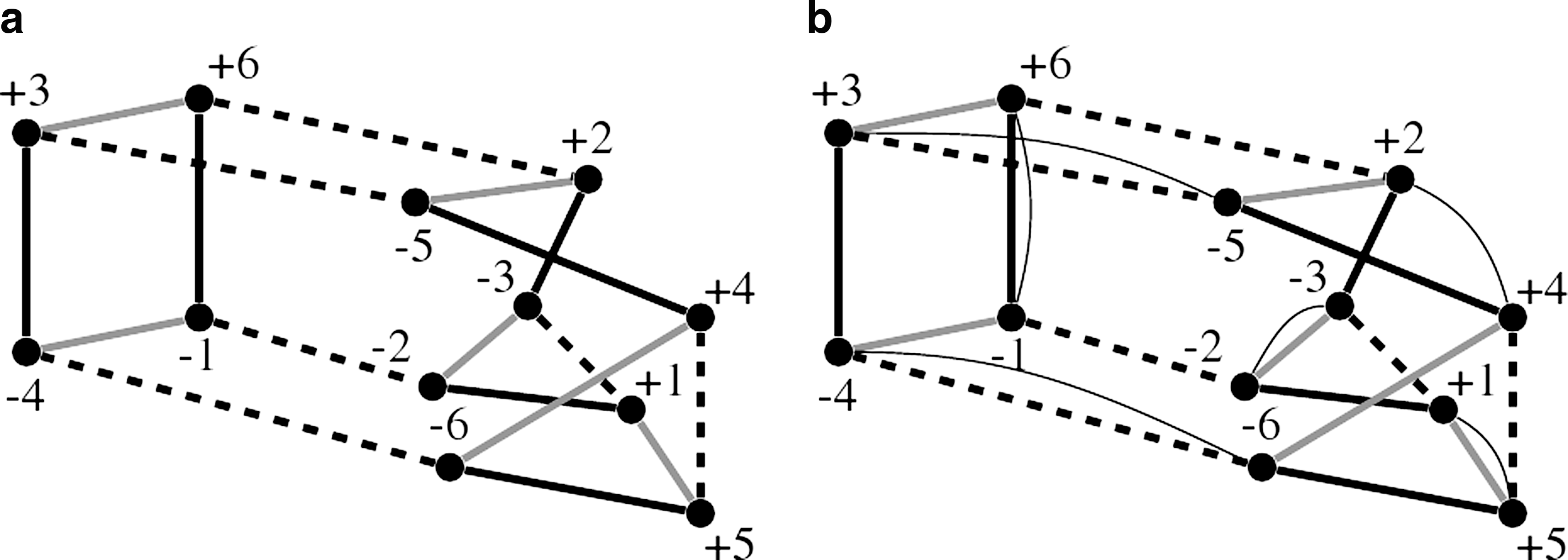
The multiple breakpoint graph (MBG) (Caprara, 2003) is a natural extension of the breakpoint graph, to represent three or more genomes (Fig. 2a). The MBG is constructed similar to the breakpoint graph: genes are represented by pairs of vertices and adjacencies between neighboring genes are represented by colored edges. We use \documentclass{aastex}\usepackage{amsbsy}\usepackage{amsfonts}\usepackage{amssymb}\usepackage{bm}\usepackage{mathrsfs}\usepackage{pifont}\usepackage{stmaryrd}\usepackage{textcomp}\usepackage{portland, xspace}\usepackage{amsmath, amsxtra}\pagestyle{empty}\DeclareMathSizes{10}{9}{7}{6}\begin{document}$$N_\mathcal {G}$$\end{document} to denote the number of given genomes in the median problem. Throughout this paper, we discuss the general case with \documentclass{aastex}\usepackage{amsbsy}\usepackage{amsfonts}\usepackage{amssymb}\usepackage{bm}\usepackage{mathrsfs}\usepackage{pifont}\usepackage{stmaryrd}\usepackage{textcomp}\usepackage{portland, xspace}\usepackage{amsmath, amsxtra}\pagestyle{empty}\DeclareMathSizes{10}{9}{7}{6}\begin{document}$$N_\mathcal {G}\, \geq\, 3$$\end{document}, except for the illustrated (capped) adequate subgraphs and the algorithm ASMeidan-linear, which are specific to the most practical case of \documentclass{aastex}\usepackage{amsbsy}\usepackage{amsfonts}\usepackage{amssymb}\usepackage{bm}\usepackage{mathrsfs}\usepackage{pifont}\usepackage{stmaryrd}\usepackage{textcomp}\usepackage{portland, xspace}\usepackage{amsmath, amsxtra}\pagestyle{empty}\DeclareMathSizes{10}{9}{7}{6}\begin{document}$$N_\mathcal {G} = 3$$\end{document}. We define the size of the MBG or its subgraphs as half the number of vertices it contains.
Multiple breakpoint graph and median graph. Black, gray, dashed, and thin edges denote edges with colors 1, 2, 3 and 0 correspondingly. (a) A multiple breakpoint graph of three circular genomes, (1 2 3 4 5 6), (1 −5 −2 3 −6 −4), and (1 3 5 −4 6 −2) (b) A median graph with the median genome (1 −5 −3 2 −4 6). “(” and “)” are used to delimit circular chromosomes.
By a i-edge we mean an edge in color i, with \documentclass{aastex}\usepackage{amsbsy}\usepackage{amsfonts}\usepackage{amssymb}\usepackage{bm}\usepackage{mathrsfs}\usepackage{pifont}\usepackage{stmaryrd}\usepackage{textcomp}\usepackage{portland, xspace}\usepackage{amsmath, amsxtra}\pagestyle{empty}\DeclareMathSizes{10}{9}{7}{6}\begin{document}$$1\, \le\, i \,\leq\, N_\mathcal {G}$$\end{document}. Since edges in the same color form a perfect matching of the MBG, we use i-matching to denote all edges of color i. For a candidate median genome, we use a different color for its adjacency edges, namely color 0; similarly we have 0-edges and 0-matchings. Adding such a candidate matching to the MBG results in the median graph (Fig. 2b). The set of all possible candidate matchings is denoted by \documentclass{aastex}\usepackage{amsbsy}\usepackage{amsfonts}\usepackage{amssymb}\usepackage{bm}\usepackage{mathrsfs}\usepackage{pifont}\usepackage{stmaryrd}\usepackage{textcomp}\usepackage{portland, xspace}\usepackage{amsmath, amsxtra}\pagestyle{empty}\DeclareMathSizes{10}{9}{7}{6}\begin{document}$$\mathcal {E}$$\end{document}.
The 0-i cycles in a median graph with a 0-matching E, numbering c0,i in all, are the cycles where 0-edges and i-edges alternate. Let \documentclass{aastex}\usepackage{amsbsy}\usepackage{amsfonts}\usepackage{amssymb}\usepackage{bm}\usepackage{mathrsfs}\usepackage{pifont}\usepackage{stmaryrd}\usepackage{textcomp}\usepackage{portland, xspace}\usepackage{amsmath, amsxtra}\pagestyle{empty}\DeclareMathSizes{10}{9}{7}{6}\begin{document}$$c^{\Sigma}_E = \Sigma_{1 \leq i \leq N_{\mathcal {G}}}c_{0,i}$$\end{document} Then \documentclass{aastex}\usepackage{amsbsy}\usepackage{amsfonts}\usepackage{amssymb}\usepackage{bm}\usepackage{mathrsfs}\usepackage{pifont}\usepackage{stmaryrd}\usepackage{textcomp}\usepackage{portland, xspace}\usepackage{amsmath, amsxtra}\pagestyle{empty}\DeclareMathSizes{10}{9}{7}{6}\begin{document}$$c^{\Sigma}_{\max} = \max \{c^{\Sigma}_E:E \in \mathcal {E}\}$$\end{document} is the maximum number of cycles that can be formed from the MBG. For circular genomes, since the DCJ distance is determined by the number of cycles in the induced breakpoint graph, we have:
Lemma 1
(Xu and Sankoff, 2008). Minimizing the total DCJ distance in the median problem on circular genomes is equivalent to finding an optimal 0-matching E, i.e., with\documentclass{aastex}\usepackage{amsbsy}\usepackage{amsfonts}\usepackage{amssymb}\usepackage{bm}\usepackage{mathrsfs}\usepackage{pifont}\usepackage{stmaryrd}\usepackage{textcomp}\usepackage{portland, xspace}\usepackage{amsmath, amsxtra}\pagestyle{empty}\DeclareMathSizes{10}{9}{7}{6}\begin{document}$$c^{\Sigma}_E = c^{\Sigma}_{\max}$$\end{document}.
A connected MBG subgraph H of size m is an adequate subgraph if \documentclass{aastex}\usepackage{amsbsy}\usepackage{amsfonts}\usepackage{amssymb}\usepackage{bm}\usepackage{mathrsfs}\usepackage{pifont}\usepackage{stmaryrd}\usepackage{textcomp}\usepackage{portland, xspace}\usepackage{amsmath, amsxtra}\pagestyle{empty}\DeclareMathSizes{10}{9}{7}{6}\begin{document}$$c^{\Sigma}_{\max} (H) \geq \frac {1}{2} mN_{\mathcal {G}}$$\end{document}; it is strongly adequate if \documentclass{aastex}\usepackage{amsbsy}\usepackage{amsfonts}\usepackage{amssymb}\usepackage{bm}\usepackage{mathrsfs}\usepackage{pifont}\usepackage{stmaryrd}\usepackage{textcomp}\usepackage{portland, xspace}\usepackage{amsmath, amsxtra}\pagestyle{empty}\DeclareMathSizes{10}{9}{7}{6}\begin{document}$$c^{\Sigma}_{\max} (H) > \frac {1}{2} mN_{\mathcal {G}}$$\end{document}. For the median of three problem with \documentclass{aastex}\usepackage{amsbsy}\usepackage{amsfonts}\usepackage{amssymb}\usepackage{bm}\usepackage{mathrsfs}\usepackage{pifont}\usepackage{stmaryrd}\usepackage{textcomp}\usepackage{portland, xspace}\usepackage{amsmath, amsxtra}\pagestyle{empty}\DeclareMathSizes{10}{9}{7}{6}\begin{document}$$N_\mathcal {G} = 3$$\end{document}, an adequate subgraph is a subgraph with \documentclass{aastex}\usepackage{amsbsy}\usepackage{amsfonts}\usepackage{amssymb}\usepackage{bm}\usepackage{mathrsfs}\usepackage{pifont}\usepackage{stmaryrd}\usepackage{textcomp}\usepackage{portland, xspace}\usepackage{amsmath, amsxtra}\pagestyle{empty}\DeclareMathSizes{10}{9}{7}{6}\begin{document}$$c^{\Sigma}_{\max} (H) \geq \frac {3m}{2}$$\end{document} and a strongly adequate subgraph is the one with \documentclass{aastex}\usepackage{amsbsy}\usepackage{amsfonts}\usepackage{amssymb}\usepackage{bm}\usepackage{mathrsfs}\usepackage{pifont}\usepackage{stmaryrd}\usepackage{textcomp}\usepackage{portland, xspace}\usepackage{amsmath, amsxtra}\pagestyle{empty}\DeclareMathSizes{10}{9}{7}{6}\begin{document}$$c^{\Sigma}_{\max} (H) > \frac {3m}{2}$$\end{document}.
The existence of an adequate subgraphs on an MBG gives an optimality-preserving decomposition of the MBG into two subproblems, where the optimal solution of the original problem can be found by combing solutions from the two subproblems, as stated in the following theorem.
Theorem 1
(Xu and Sankoff, 2008).1The existence of an adequate subgraph gives an optimality-preserving decomposition from which an optimal solution can be found by combining solutions from the two subproblems. The existence of a strongly adequate subgraph gives a proper decomposition from which all optimal solutions can be found by combining solutions from the two subproblems.
Remark 1
Subproblems induced by adequate subgraphs of small sizes are easy to solve. When we only use these small adequate subgraphs, we can encode their solutions into algorithms, so that whenever their existences are detected, adjacencies representing solutions of these subproblems are immediately added into the median genome.
3. Capped Multiple Breakpoint Graph—A Graph Representation of the Median Problem on Linear Multichromosomal Genomes
Existing median solvers cleverly use pairwise genomic distance to guide iterative procedures in finding median genomes. Instead, our adequate-subgraph based method on circular genomes detects patterns in the given genomes, which directly tell us how to construct the median genome. Before we extend this method to linear multichromosomal genomes, we need an appropriate graph representation which should satisfy the following requirements: both complete and partial median genomes (the intermediate solution to the median problem with missing adjacencies) can be represented unambiguously, and after adding each 0-edge the size of the graph will be reduced by one.
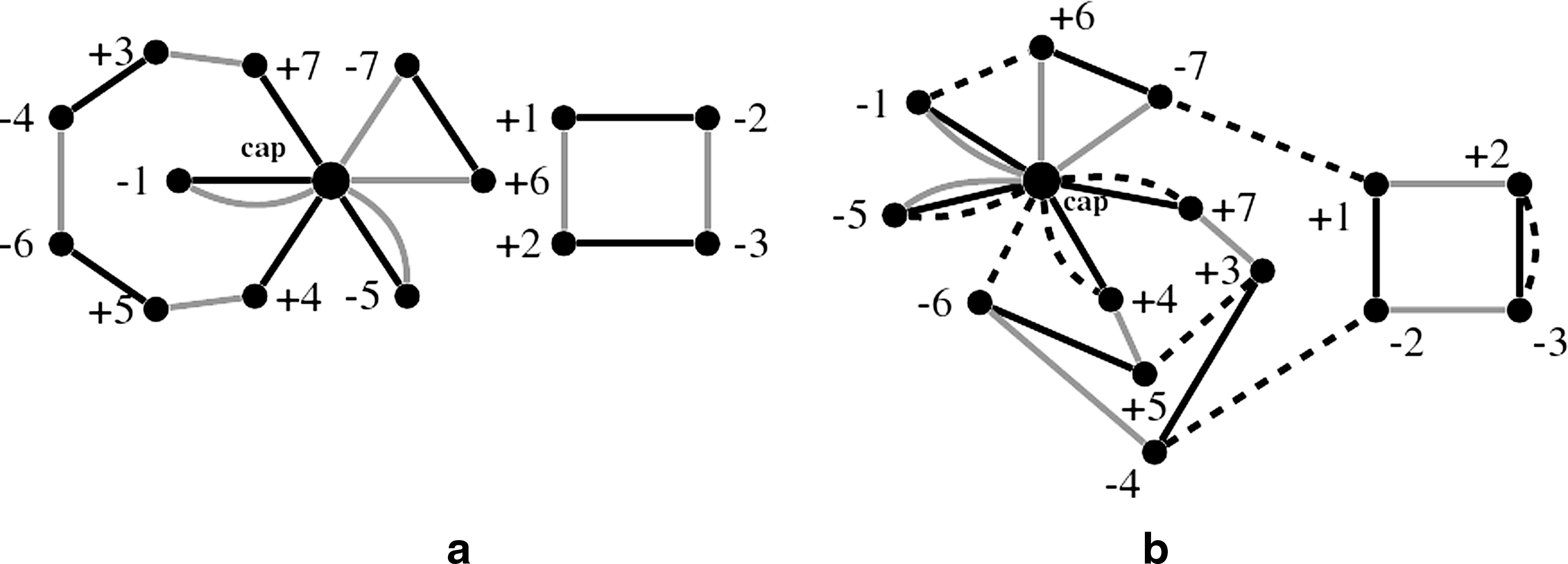
Alekseyev and Pevzner (2009) introduced their version of multiple breakpoint graph (Fig. 3b) on linear genomes for the ancestral genome reconstruction problem on a given phylogeny. They used an infinity node (∞) to delimit all ends of linear chromosomes, which is similar to the single cap node in the flower graph (Xu, 2007; Fig. 3a) for pairwise genomes. Their multiple breakpoint graph can unambiguously represent both complete and partial genomes, and supports a size reduction operation.
(a) Flower graph for genomes {1 2 3 4; 5 6 7} and {1 −2 3 −7; 5 −4 6}, where we use black and gray edges to distinguish adjacency edges from different genomes. We have n = 7, χ = 2, c = 1, po = 2, pe = 2, so their DCJ distance is 5. (b) The multiple breakpoint graph introduced in Alekseyev and Pevzner (2009) for the three genomes {1 2 3 4; 5 6 7}, {1 −2 3 −7; 5 −4 6}, and {5 −3 −2 4; 6 1 7}. Black, gray, and dashed edges represent edges of colors 1 2 and 3, correspondingly. The cap is incident to 6 edges.
However, their graph representation and the ancestral reconstruction problem have the following three differences with our problem. (1) The genomes represented in their graph are assigned a certain phylogeny structure which does no exist in our median problem. (2) Their heuristic algorithm searches for good rearrangements to iteratively reduce the difference among genomes, and our exact method iteratively constructs the adjacencies (the 0-edges) for the median genome. (3) Their size reduction operation is not quite the same as our shrinking operation: in their method, the size of the graph is reduced, if after applying good rearrangements some adjacencies appear in all genomes; in our method, the size is reduced when 0-edges are added, regardless of the adjacencies in the given genomes. (See Figure 4 for the shrinking operation. Caprara [2003] calls it a “contraction”; and in order to distinguish it from a terminology in graph theory which has the same name but different meaning, Xu and Sankoff [2008] calls it a “shrinking.)”
A shrinking operation on a 0-edge is, to remove the 0-edge together with any possible edges parallel edges and its two endpoints, and to merge the pairs of edges in the same colors. (a) A 0-edge and its adjacent edges in the MBG. If we decompose the multiple breakpoint graph into three corresponding (incomplete) breakpoint graphs (b), the shrinking operation is equivalent to removing bi-colored cycles and to replacing bi-colored paths by single edges (c). The size of the resultant MBG is smaller by one.
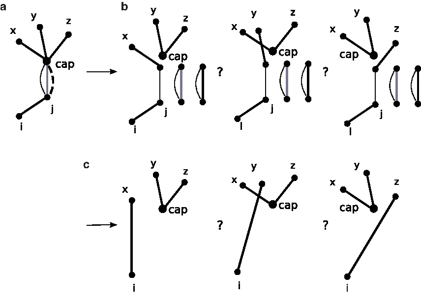
The first difference disappears when the number of genomes is 3, as the first problem also becomes a median problem. The second and the third differences lead to a problem, if the same graph is used in our exact method: if the added 0-edge is incident to the infinity node (we will call it the cap node in our graph representation, following the tradition in Hannenhalli and Pevzner [1995b] and Tesler [2002]), it is not possible to reduce the size of the graph and maintain the optimality of the problem. This difficulty is shown in Figure 5, as there are more than one solid edge incident to the cap node, we do not know which one we should perform the shrinking operation with.
Shrinking 0-edges incident to the cap node causes a problem. When such an edge presents (a), it leads to different possible corresponding breakpoint graphs (b) and thus different resultant CMBGs (c).
3.1. Capped multiple breakpoint graph
We then introduce the capped multiple breakpoint graph (CMBG) to solve the problem in size reduction. The vertices in the CMBG consist of vertices representing ends of genes (which are called regular vertices), a single cap node to delimit the ends of all chromosomes, and a single cup node to help to solve the problem in shrinking. Each genome together with the edges representing its adjacencies is assigned a unique color, the edges (regular edges) connecting regular vertices represent adjacencies between genes, and the edges (cap edges) connecting regular vertices to the cap node represent adjacencies between ends of linear chromosomes and the first/last genes in the corresponding chromosomes.
If the given genomes do not have the same number of linear chromosomes, null chromosomes consisting of no genes and being delimited by the cap node are added, so that the numbers of linear chromosomes are equal. These null chromosomes are represented by edges looping around the cap node. As discussed in Yancopoulos et al. (2005) and Bergeron et al. (2006), adding null chromosomes does not change the pairwise distance, and hence it does not change the total distance of the median problem either. Before any 0-edge is added, the cup node is an isolated vertex. Figure 6 shows the CMBG for three linear multichromosomal genomes: {1 2 3 4; 5 6 7}, {1 −2 3 −7; 5 −4 6}, and {5 −3 −2 4; 6 1 7}.
(a) Capped multiple breakpoint graph. (b) The consequent graph after three edges (+4, cap), (+7, cap), and (−7, cap) are shrunk. Solid, gray, and dashed edges are used to represent adjacencies for the three genomes respectively.
When a regular 0-edge is added into the CMBG, it connects pairs of edges in the same colors or two ends of the same edges. These pairs of edges belong to the same bi-colored cycles or paths in the corresponding breakpoint graphs between the median genome and the given genomes, and the edges with both endpoints connected by the 0-edge form bi-colored cycles, as shown in Figure 4b. When a 0 cap edge is added there is a problem, because we do not know which pairs of edges should belong to the same bi-colored cycles or paths in the corresponding breakpoint graph(s), as shown in Figure 5b.
The introduction of the cup node provides a means for us to represent the ambiguity in shrinking a 0 cap edge, and to delay resolving this ambiguity until we know how to resolve it optimally. The shrinking operation on the CMBG is illustrated by Figure 7. When a 0 cap edge is added to the CMBG (in subfigure (a)), we can not perform a regular shrinking because of the existence of edge (i, j). Subfigure (b) shows the relevant part of the corresponding three incomplete breakpoint graphs (flower graphs, indeed). In subfigure (c), bi-colored cycles are removed, vertex j is deleted, edge (i, j)—which has only one endpoint now—is connected to the cup node, and so is the 0 cap edge. In subfigure (d), the 0 cap edge is omitted for the purpose of simplicity; omitting these edges does not cause confusion, as the number of these omitted 0 cap edges is equal to the number of edges incident to the cup node. Hence the cup node collects the edges with ambiguity and allows us to delay the decisions on them until we know how. Subfigure (e) shows the resultant graph after more 0 cap edges are added and shrunk.
An illustration of the shrinking operation on CMBG when the cup node is introduced. (a) A 0 cap edge presents on a CMBG. (b) In the corresponding breakpoint graphs (flower graphs, indeed), ambiguity exists and we do not intend to resolve it immediately. (c) Under the shrinking operation on a CMBG, bi-colored cycles are removed, vertex j is deleted, edge (i, j)—which has only one endpoint now—is connected to the cup node, and so is the 0 cap edge. (d) The 0-edge between the cap and the cup nodes are omitted. (e) When more 0 cap edges show up, the cup node collects more edges with ambiguity.
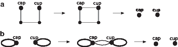
As more 0 cap edges are added and shrunk, there will be more edges incident to the cup node. There are two situations, in which we can resolve the ambiguity on these edges and decrease their number. These two situations are shown by Figure 8.
Two situations to resolve the ambiguity due to shrinking 0 cap edges. (a) When a 0-edge connects two edges in the same color incident to the cap node and the cup node respectively, we see a cycle of size 4, after we restore the omitted 0-edge between the cap and the cup. It is clear this cap-edge should be included in the cycle containing the edge incident to the cup node. The ambiguity on this edge is resolved. In the corresponding breakpoint graph, the cap edge, the edge incident to the cup node and the newly added 0-edge form an even path, which can form a cycle by itself. (b) When two loops in the same color form at the cap node and the cup node respectively, we also see a cycle of size 4, after we restore the two omitted 0-edges between the cap and the cup. These two loops, in the corresponding breakpoint graph, represent two odd paths of different types, and they form one cycle. In both situations, the size of the graph decreases by one; the number of edges incident to the cup node decreases by one or two respectively.
When an edge e1 incident to the cup node is connected to a cap edge e2 by a newly added 0-edge, in subfigure (a), the three edges plus an omitted 0 cap edge between the cap and the cup nodes form a bi-colored cycle. Indeed, this is an even-sized bi-colored path in its breakpoint graph. According to Theorem 3 presented in Section 4, pairing up edges e1 and e2 is an optimal choice. Then the ambiguity on e1 is resolved, and e1 together with e2 can be removed from CMBG.
Subfigure (b) shows another situation, where the cap and the cup nodes each have a loop in the same color. In the corresponding breakpoint graph, each loop represents an odd-sized bi-colored path. It is easy to see that the optimal choice is to connect the two loops (paths) by two omitted 0 cap edges between the cap and the cup nodes to form one bi-colored cycle.
Suppose the median problem contains \documentclass{aastex}\usepackage{amsbsy}\usepackage{amsfonts}\usepackage{amssymb}\usepackage{bm}\usepackage{mathrsfs}\usepackage{pifont}\usepackage{stmaryrd}\usepackage{textcomp}\usepackage{portland, xspace}\usepackage{amsmath, amsxtra}\pagestyle{empty}\DeclareMathSizes{10}{9}{7}{6}\begin{document}$$N_\mathcal {G}$$\end{document} genomes, each with n genes and χ linear chromosomes (null chromosomes are added if necessary). In the CMBG, each of the 2n regular vertices representing genes is incident to exact \documentclass{aastex}\usepackage{amsbsy}\usepackage{amsfonts}\usepackage{amssymb}\usepackage{bm}\usepackage{mathrsfs}\usepackage{pifont}\usepackage{stmaryrd}\usepackage{textcomp}\usepackage{portland, xspace}\usepackage{amsmath, amsxtra}\pagestyle{empty}\DeclareMathSizes{10}{9}{7}{6}\begin{document}$$N_\mathcal {G}$$\end{document} edges with \documentclass{aastex}\usepackage{amsbsy}\usepackage{amsfonts}\usepackage{amssymb}\usepackage{bm}\usepackage{mathrsfs}\usepackage{pifont}\usepackage{stmaryrd}\usepackage{textcomp}\usepackage{portland, xspace}\usepackage{amsmath, amsxtra}\pagestyle{empty}\DeclareMathSizes{10}{9}{7}{6}\begin{document}$$N_\mathcal {G}$$\end{document} different colors, and the cap node is incident to \documentclass{aastex}\usepackage{amsbsy}\usepackage{amsfonts}\usepackage{amssymb}\usepackage{bm}\usepackage{mathrsfs}\usepackage{pifont}\usepackage{stmaryrd}\usepackage{textcomp}\usepackage{portland, xspace}\usepackage{amsmath, amsxtra}\pagestyle{empty}\DeclareMathSizes{10}{9}{7}{6}\begin{document}$$\chi N_\mathcal {G}$$\end{document} edges, where each possible looping edge is counted twice.
The size of a CMBG or its subgraph is an important parameter in defining (cap) adequate subgraphs in the next section. The size of a CMBG is simply n + χ. The definition for a subgraph is a little bit complicated. Let δi be the number of edges in color i which are incident to the cap node. Then let δ be the maximum of these δi with \documentclass{aastex}\usepackage{amsbsy}\usepackage{amsfonts}\usepackage{amssymb}\usepackage{bm}\usepackage{mathrsfs}\usepackage{pifont}\usepackage{stmaryrd}\usepackage{textcomp}\usepackage{portland, xspace}\usepackage{amsmath, amsxtra}\pagestyle{empty}\DeclareMathSizes{10}{9}{7}{6}\begin{document}$$1 \,\le\, i \,\le\, N_\mathcal {G}$$\end{document}. For a subgraph not containing the cap node, we simply let δ = 0. Let s be the number of regular vertices in this subgraph. Then the size of a CMBG subgraph, m, is defined as:
\documentclass{aastex}\usepackage{amsbsy}\usepackage{amsfonts}\usepackage{amssymb}\usepackage{bm}\usepackage{mathrsfs}\usepackage{pifont}\usepackage{stmaryrd}\usepackage{textcomp}\usepackage{portland, xspace}\usepackage{amsmath, amsxtra}\pagestyle{empty}\DeclareMathSizes{10}{9}{7}{6}\begin{document}\begin{align*}m = \frac {s + \delta}{2}.\tag{2}\end{align*}\end{document}
The size of the CMBG or its subgraph tells the maximum number of 0-edges we can add. On general subgraphs, δ + s may take odd values; but for (capped) adequate subgraphs, it is always even.
Similar to Lemma 1 we have the following statement for the median problem on linear multichromosomal genomes.
Lemma 2
Finding the DCJ median on\documentclass{aastex}\usepackage{amsbsy}\usepackage{amsfonts}\usepackage{amssymb}\usepackage{bm}\usepackage{mathrsfs}\usepackage{pifont}\usepackage{stmaryrd}\usepackage{textcomp}\usepackage{portland, xspace}\usepackage{amsmath, amsxtra}\pagestyle{empty}\DeclareMathSizes{10}{9}{7}{6}\begin{document}$$N_\mathcal {G}$$\end{document}genomes with n genes and χ linear chromosomes is equivalent to finding a set of n + χ 0-edges E for the capped multiple breakpoint graph, satisfying the following properties:
1. each regular vertex is incident to E exactly once;
2. the cap node is incident to E exactly 2χ times;
3. E maximizes\documentclass{aastex}\usepackage{amsbsy}\usepackage{amsfonts}\usepackage{amssymb}\usepackage{bm}\usepackage{mathrsfs}\usepackage{pifont}\usepackage{stmaryrd}\usepackage{textcomp}\usepackage{portland, xspace}\usepackage{amsmath, amsxtra}\pagestyle{empty}\DeclareMathSizes{10}{9}{7}{6}\begin{document}$$\Sigma_{1 \le i \le N_{\mathcal N}} {\hat c}_{0,i}$$\end{document}, where\documentclass{aastex}\usepackage{amsbsy}\usepackage{amsfonts}\usepackage{amssymb}\usepackage{bm}\usepackage{mathrsfs}\usepackage{pifont}\usepackage{stmaryrd}\usepackage{textcomp}\usepackage{portland, xspace}\usepackage{amsmath, amsxtra}\pagestyle{empty}\DeclareMathSizes{10}{9}{7}{6}\begin{document}$${\hat c}_{0,i}$$\end{document}is equal to\documentclass{aastex}\usepackage{amsbsy}\usepackage{amsfonts}\usepackage{amssymb}\usepackage{bm}\usepackage{mathrsfs}\usepackage{pifont}\usepackage{stmaryrd}\usepackage{textcomp}\usepackage{portland, xspace}\usepackage{amsmath, amsxtra}\pagestyle{empty}\DeclareMathSizes{10}{9}{7}{6}\begin{document}$$c + p_e + \frac{p_o}{2}$$\end{document}in the breakpoint graph of the candidate median genome and the given genome i.
3.2. Capping revisited and the multi-way capping optimization problem
Using a single cap node in the CMBG follows the idea of using a pair of caps to delimit each linear chromosome in Hannenhalli and Pevzner (1995b) and Tesler (2002). The caps can be understood as the representation of telomeres located at the ends of linear chromosomes. If we knew the “orthology relationship” of these telomeres across species, we then could assign these caps unique labels. And this is called a capping. Then in the corresponding graph representation, each vertex (either a regular vertex or a cap) would be incident to one edge from each genome, and this would be an MBG representing the median problem on circular genomes. Then we could solve this problem by ASMedian developed in Xu and Sankoff (2008).
But we do not know this “orthology relationship.” Alternatively, we can search among all possible cappings to find the one which gives the smallest total distance: this is a multi-way capping optimization problem. It took a lot of efforts to solve the two-way capping optimization problem (Hannenhalli and Pevzner, 1995b; Tesler, 2002; Ozery-Flato and Shamir, 2003; Jean and Nikolski, 2007) in computing the HP distance between two linear multichromosomal genomes. The multi-way capping optimization problem coupled with the median problem is unlikely to be solved in polynomial time. If there are \documentclass{aastex}\usepackage{amsbsy}\usepackage{amsfonts}\usepackage{amssymb}\usepackage{bm}\usepackage{mathrsfs}\usepackage{pifont}\usepackage{stmaryrd}\usepackage{textcomp}\usepackage{portland, xspace}\usepackage{amsmath, amsxtra}\pagestyle{empty}\DeclareMathSizes{10}{9}{7}{6}\begin{document}$$N_\mathcal {G}$$\end{document} given genomes in the median problem and each genome has χ linear chromosomes, we can fix the labels in the first genome and try all (2χ)! ways to assign labels to each of the remaining \documentclass{aastex}\usepackage{amsbsy}\usepackage{amsfonts}\usepackage{amssymb}\usepackage{bm}\usepackage{mathrsfs}\usepackage{pifont}\usepackage{stmaryrd}\usepackage{textcomp}\usepackage{portland, xspace}\usepackage{amsmath, amsxtra}\pagestyle{empty}\DeclareMathSizes{10}{9}{7}{6}\begin{document}$$N_\mathcal {G} - 1$$\end{document} genomes. Thus the total number of unique cappings is \documentclass{aastex}\usepackage{amsbsy}\usepackage{amsfonts}\usepackage{amssymb}\usepackage{bm}\usepackage{mathrsfs}\usepackage{pifont}\usepackage{stmaryrd}\usepackage{textcomp}\usepackage{portland, xspace}\usepackage{amsmath, amsxtra}\pagestyle{empty}\DeclareMathSizes{10}{9}{7}{6}\begin{document}$$((2\chi)!)^{N_\mathcal {G} - 1}$$\end{document}. This number grows explosively with χ. When \documentclass{aastex}\usepackage{amsbsy}\usepackage{amsfonts}\usepackage{amssymb}\usepackage{bm}\usepackage{mathrsfs}\usepackage{pifont}\usepackage{stmaryrd}\usepackage{textcomp}\usepackage{portland, xspace}\usepackage{amsmath, amsxtra}\pagestyle{empty}\DeclareMathSizes{10}{9}{7}{6}\begin{document}$$N_\mathcal {G} = 3$$\end{document} and χ = 23, the number of chromosomes in human genome, there are 3.03 × 10115 different cappings. So it is prohibitive to enumerate all of them and to solve the corresponding equivalent median problems on circular genomes. We have to solve this multi-way capping optimization problem together with the median problem on linear multichromosomal genomes by exploring the patterns in the given genomes to progressively rule out non-optimal cappings. And this is the motivation of this paper.
On the other hand, if we know the median genome, the multi-way capping optimization problem can be decomposed into \documentclass{aastex}\usepackage{amsbsy}\usepackage{amsfonts}\usepackage{amssymb}\usepackage{bm}\usepackage{mathrsfs}\usepackage{pifont}\usepackage{stmaryrd}\usepackage{textcomp}\usepackage{portland, xspace}\usepackage{amsmath, amsxtra}\pagestyle{empty}\DeclareMathSizes{10}{9}{7}{6}\begin{document}$$N_\mathcal {G}$$\end{document} pairwise capping optimization problems, which we can solve efficiently (Yancopoulos et al., 2005; Xu, 2007).
4. The Decomposition Theorems and Adequate Subgraphs
For the median problem on circular genomes, Xu and Sankoff (2008) show that existences of adequate subgraphs allows us to decompose the problem into two subproblems from which the optimal solution of the original problem can be found by combining solutions to the two subproblems. In this section, we will develop the parallel results for the problem on linear multichromosomal genomes. The cap node in the capped multiple breakpoint graph requires us to distinguish two types of subgraphs: regular subgraphs—the ones not containing the cap node; capped subgraphs—the ones containing the cap node. Parallel to these definitions, we have two types of adequate subgraphs: regular adequate subgraphs and capped adequate subgraphs. The following theorem, with no surprise, states that regular adequate subgraphs defined on CMBGs are isomorphic to adequate subgraphs defined on MBGs. Figure 9I shows the most frequent ones (Xu and Sankoff, 2008).
The most frequent (I) regular adequate subgraphs (Xu and Sankoff, 2008) and (II) capped adequate subgraphs on CMBGs. Black, gray and dashed edges represent adjacency edges from given genomes and thin edges represent adjacency edge in the median genome.
Theorem 2
As long as the cap node is not involved, regular adequate subgraphs are applicable to capped multiple breakpoint graphs, giving optimality-preserving decompositions.
Proof
If we use 2χ caps to delimiter χ linear chromosomes in a traditional way and treat these caps as regular vertices (as these caps are all of degree \documentclass{aastex}\usepackage{amsbsy}\usepackage{amsfonts}\usepackage{amssymb}\usepackage{bm}\usepackage{mathrsfs}\usepackage{pifont}\usepackage{stmaryrd}\usepackage{textcomp}\usepackage{portland, xspace}\usepackage{amsmath, amsxtra}\pagestyle{empty}\DeclareMathSizes{10}{9}{7}{6}\begin{document}$$N_\mathcal {G}$$\end{document}), each CMBG can be transformed into \documentclass{aastex}\usepackage{amsbsy}\usepackage{amsfonts}\usepackage{amssymb}\usepackage{bm}\usepackage{mathrsfs}\usepackage{pifont}\usepackage{stmaryrd}\usepackage{textcomp}\usepackage{portland, xspace}\usepackage{amsmath, amsxtra}\pagestyle{empty}\DeclareMathSizes{10}{9}{7}{6}\begin{document}$$((2\chi)!)^{N_\mathcal {G}}$$\end{document} MBGs, according to different cappings of caps. Suppose a regular adequate subgraph exists on the CMBG, then it must also exist in every MBG, as the transformation between the CMBG and the MBGs does not change regular vertices or edges connecting them. This adequate subgraph then decomposes every MBG into two parts, one of which is the adequate subgraph itself. Then the same optimality-preserving decomposition induced by this adequate subgraph must exist on the original CMBG. ▪
For capped subgraphs allowing optimality-preserving decompositions, we expect the following three categories, according to the kinds of solutions the induced decompositions lead to:
the ones leading to all optimal solutions and all possible optimal cappings;
the ones leading to some optimal solutions and all possible optimal cappings;
the ones leading to some optimal solutions and some optimal capping.
In this article, we give definitions to capped adequate subgraphs of the first two categories; they are similar to strongly adequate subgraphs and adequate subgraphs on MBGs respectively. But first let us quickly review some relevant definitions.
Recall that the size of a subgraph is \documentclass{aastex}\usepackage{amsbsy}\usepackage{amsfonts}\usepackage{amssymb}\usepackage{bm}\usepackage{mathrsfs}\usepackage{pifont}\usepackage{stmaryrd}\usepackage{textcomp}\usepackage{portland, xspace}\usepackage{amsmath, amsxtra}\pagestyle{empty}\DeclareMathSizes{10}{9}{7}{6}\begin{document}$$\frac {s + \delta}{2}$$\end{document}, where s is the number of regular vertices in the subgraph and δ is the maximum number of cap edges in the same color in the subgraph. Define γ as the total number of cap edges in the subgraph. For a CMBG subgraph H, \documentclass{aastex}\usepackage{amsbsy}\usepackage{amsfonts}\usepackage{amssymb}\usepackage{bm}\usepackage{mathrsfs}\usepackage{pifont}\usepackage{stmaryrd}\usepackage{textcomp}\usepackage{portland, xspace}\usepackage{amsmath, amsxtra}\pagestyle{empty}\DeclareMathSizes{10}{9}{7}{6}\begin{document}$${\hat c}^{\Sigma}_{\max}(H)$$\end{document} is the maximum bi-colored cycles formed by a set of 0-edges with H.
Definition 1
A capped adequate subgraph is a connected capped subgraph H of size m with\documentclass{aastex}\usepackage{amsbsy}\usepackage{amsfonts}\usepackage{amssymb}\usepackage{bm}\usepackage{mathrsfs}\usepackage{pifont}\usepackage{stmaryrd}\usepackage{textcomp}\usepackage{portland, xspace}\usepackage{amsmath, amsxtra}\pagestyle{empty}\DeclareMathSizes{10}{9}{7}{6}\begin{document}$${\hat c}^{\Sigma}_{max}(H)\,\geq\,\frac {1}{2}(mN_ \mathcal {G} + \gamma - \delta)$$\end{document}.
Definition 2
A capped strongly adequate subgraph is a connected capped subgraph H of size m with\documentclass{aastex}\usepackage{amsbsy}\usepackage{amsfonts}\usepackage{amssymb}\usepackage{bm}\usepackage{mathrsfs}\usepackage{pifont}\usepackage{stmaryrd}\usepackage{textcomp}\usepackage{portland, xspace}\usepackage{amsmath, amsxtra}\pagestyle{empty}\DeclareMathSizes{10}{9}{7}{6}\begin{document}$${\hat c}^{\Sigma}_{max}(H) > \frac {1}{2}(mN_ {calG} + \gamma - \delta)$$\end{document}.
It is worthwhile to note that the parameter γ on any capped adequate subgraph is larger than 1, because vertex degrees on any adequate subgraphs are at least 2 (Xu, 2008). A simple capped (strongly) adequate subgraph is the capped (strongly) subgraph for which none of its induced subgraph is an adequate subgraph or a capped adequate subgraph. Figure 9II shows the most frequent simple capped adequate subgraphs.
Theorem 3
The existence of a capped adequate subgraph on a CMBG gives an optimality-preserving decomposition from which an optimal solution can be found by combining solutions to the two subproblems. The existence of a capped strongly adequate subgraph gives an optimality-preserving decomposition from which all optimal solutions can be found by combining solutions to the two subproblems.
Proof
Suppose in the capped adequate subgraph H of size m, there are γ cap edges and the maximum number of cap edges in the same color is δ. Without loss of generality, we assume this maximum is obtained by cap edges of color 1.
In this proof, we explicitly consider the cappings of caps. We denote the global optimal capping, the solution to the capping optimization problem, as \documentclass{aastex}\usepackage{amsbsy}\usepackage{amsfonts}\usepackage{amssymb}\usepackage{bm}\usepackage{mathrsfs}\usepackage{pifont}\usepackage{stmaryrd}\usepackage{textcomp}\usepackage{portland, xspace}\usepackage{amsmath, amsxtra}\pagestyle{empty}\DeclareMathSizes{10}{9}{7}{6}\begin{document}$$\mathcal {GL}$$\end{document}. We denote a second capping, which is local optimal on the caps involved in H, as \documentclass{aastex}\usepackage{amsbsy}\usepackage{amsfonts}\usepackage{amssymb}\usepackage{bm}\usepackage{mathrsfs}\usepackage{pifont}\usepackage{stmaryrd}\usepackage{textcomp}\usepackage{portland, xspace}\usepackage{amsmath, amsxtra}\pagestyle{empty}\DeclareMathSizes{10}{9}{7}{6}\begin{document}$$\mathcal {LL}$$\end{document}. We assume, contradictory to the conclusion to the theorem, that no optimal solution to the median problem contains the local optimal solution D to the capped adequate subgraph. We will show that from any of optimal solution E not containing D, we can construct another solution E′ that contains D and has no less cycles than E.
Assume we fix the labels of the caps in genome 1 and use them to label the caps in the other two genomes. So \documentclass{aastex}\usepackage{amsbsy}\usepackage{amsfonts}\usepackage{amssymb}\usepackage{bm}\usepackage{mathrsfs}\usepackage{pifont}\usepackage{stmaryrd}\usepackage{textcomp}\usepackage{portland, xspace}\usepackage{amsmath, amsxtra}\pagestyle{empty}\DeclareMathSizes{10}{9}{7}{6}\begin{document}$$\mathcal {GL}$$\end{document} and \documentclass{aastex}\usepackage{amsbsy}\usepackage{amsfonts}\usepackage{amssymb}\usepackage{bm}\usepackage{mathrsfs}\usepackage{pifont}\usepackage{stmaryrd}\usepackage{textcomp}\usepackage{portland, xspace}\usepackage{amsmath, amsxtra}\pagestyle{empty}\DeclareMathSizes{10}{9}{7}{6}\begin{document}$$\mathcal {LL}$$\end{document} only differ on the caps in the rest \documentclass{aastex}\usepackage{amsbsy}\usepackage{amsfonts}\usepackage{amssymb}\usepackage{bm}\usepackage{mathrsfs}\usepackage{pifont}\usepackage{stmaryrd}\usepackage{textcomp}\usepackage{portland, xspace}\usepackage{amsmath, amsxtra}\pagestyle{empty}\DeclareMathSizes{10}{9}{7}{6}\begin{document}$$N_\mathcal {G} - 1$$\end{document}. Of the γ caps in the subgraph H, γ − δ caps are from these genome. On all these caps, \documentclass{aastex}\usepackage{amsbsy}\usepackage{amsfonts}\usepackage{amssymb}\usepackage{bm}\usepackage{mathrsfs}\usepackage{pifont}\usepackage{stmaryrd}\usepackage{textcomp}\usepackage{portland, xspace}\usepackage{amsmath, amsxtra}\pagestyle{empty}\DeclareMathSizes{10}{9}{7}{6}\begin{document}$$\mathcal {GL}$$\end{document} and \documentclass{aastex}\usepackage{amsbsy}\usepackage{amsfonts}\usepackage{amssymb}\usepackage{bm}\usepackage{mathrsfs}\usepackage{pifont}\usepackage{stmaryrd}\usepackage{textcomp}\usepackage{portland, xspace}\usepackage{amsmath, amsxtra}\pagestyle{empty}\DeclareMathSizes{10}{9}{7}{6}\begin{document}$$\mathcal {LL}$$\end{document} have at most γ − δ differences. Then by at most γ − δ DCJ operations (translocations operations, to be specific), we can transform \documentclass{aastex}\usepackage{amsbsy}\usepackage{amsfonts}\usepackage{amssymb}\usepackage{bm}\usepackage{mathrsfs}\usepackage{pifont}\usepackage{stmaryrd}\usepackage{textcomp}\usepackage{portland, xspace}\usepackage{amsmath, amsxtra}\pagestyle{empty}\DeclareMathSizes{10}{9}{7}{6}\begin{document}$$\mathcal {GL}$$\end{document} to another capping \documentclass{aastex}\usepackage{amsbsy}\usepackage{amsfonts}\usepackage{amssymb}\usepackage{bm}\usepackage{mathrsfs}\usepackage{pifont}\usepackage{stmaryrd}\usepackage{textcomp}\usepackage{portland, xspace}\usepackage{amsmath, amsxtra}\pagestyle{empty}\DeclareMathSizes{10}{9}{7}{6}\begin{document}$$\mathcal {L}$$\end{document} which agrees with \documentclass{aastex}\usepackage{amsbsy}\usepackage{amsfonts}\usepackage{amssymb}\usepackage{bm}\usepackage{mathrsfs}\usepackage{pifont}\usepackage{stmaryrd}\usepackage{textcomp}\usepackage{portland, xspace}\usepackage{amsmath, amsxtra}\pagestyle{empty}\DeclareMathSizes{10}{9}{7}{6}\begin{document}$$\mathcal {LL}$$\end{document} on the caps in H. Since each DCJ (translocation) operation reduces at most by one the number of cycles in the three corresponding breakpoint graphs between the median genome E and the given genomes. The maximum number of total cycles under capping \documentclass{aastex}\usepackage{amsbsy}\usepackage{amsfonts}\usepackage{amssymb}\usepackage{bm}\usepackage{mathrsfs}\usepackage{pifont}\usepackage{stmaryrd}\usepackage{textcomp}\usepackage{portland, xspace}\usepackage{amsmath, amsxtra}\pagestyle{empty}\DeclareMathSizes{10}{9}{7}{6}\begin{document}$$\mathcal {L}$$\end{document} is at most smaller by γ − δ than the total number of cycles under \documentclass{aastex}\usepackage{amsbsy}\usepackage{amsfonts}\usepackage{amssymb}\usepackage{bm}\usepackage{mathrsfs}\usepackage{pifont}\usepackage{stmaryrd}\usepackage{textcomp}\usepackage{portland, xspace}\usepackage{amsmath, amsxtra}\pagestyle{empty}\DeclareMathSizes{10}{9}{7}{6}\begin{document}$$\mathcal {GL}$$\end{document}. Note that, the optimal solution E itself is not effected by the changes from \documentclass{aastex}\usepackage{amsbsy}\usepackage{amsfonts}\usepackage{amssymb}\usepackage{bm}\usepackage{mathrsfs}\usepackage{pifont}\usepackage{stmaryrd}\usepackage{textcomp}\usepackage{portland, xspace}\usepackage{amsmath, amsxtra}\pagestyle{empty}\DeclareMathSizes{10}{9}{7}{6}\begin{document}$$\mathcal {GL}$$\end{document} to \documentclass{aastex}\usepackage{amsbsy}\usepackage{amsfonts}\usepackage{amssymb}\usepackage{bm}\usepackage{mathrsfs}\usepackage{pifont}\usepackage{stmaryrd}\usepackage{textcomp}\usepackage{portland, xspace}\usepackage{amsmath, amsxtra}\pagestyle{empty}\DeclareMathSizes{10}{9}{7}{6}\begin{document}$$\mathcal {L}$$\end{document}, although its optimality is not preserved under \documentclass{aastex}\usepackage{amsbsy}\usepackage{amsfonts}\usepackage{amssymb}\usepackage{bm}\usepackage{mathrsfs}\usepackage{pifont}\usepackage{stmaryrd}\usepackage{textcomp}\usepackage{portland, xspace}\usepackage{amsmath, amsxtra}\pagestyle{empty}\DeclareMathSizes{10}{9}{7}{6}\begin{document}$$\mathcal {L}$$\end{document}.
By replacing the corresponding 0-edges in E by D, we can show that the new solution E′ contains at least \documentclass{aastex}\usepackage{amsbsy}\usepackage{amsfonts}\usepackage{amssymb}\usepackage{bm}\usepackage{mathrsfs}\usepackage{pifont}\usepackage{stmaryrd}\usepackage{textcomp}\usepackage{portland, xspace}\usepackage{amsmath, amsxtra}\pagestyle{empty}\DeclareMathSizes{10}{9}{7}{6}\begin{document}$$2 \times \frac {1}{2} (mN_ \mathcal {G} + \gamma - \delta) - mN_\mathcal {G} = \gamma - \delta$$\end{document} more cycles than E under the capping \documentclass{aastex}\usepackage{amsbsy}\usepackage{amsfonts}\usepackage{amssymb}\usepackage{bm}\usepackage{mathrsfs}\usepackage{pifont}\usepackage{stmaryrd}\usepackage{textcomp}\usepackage{portland, xspace}\usepackage{amsmath, amsxtra}\pagestyle{empty}\DeclareMathSizes{10}{9}{7}{6}\begin{document}$$\mathcal {L}$$\end{document}, following the steps in the proof to Theorem 1 in Xu and Sankoff [2008]. From the fact that E under \documentclass{aastex}\usepackage{amsbsy}\usepackage{amsfonts}\usepackage{amssymb}\usepackage{bm}\usepackage{mathrsfs}\usepackage{pifont}\usepackage{stmaryrd}\usepackage{textcomp}\usepackage{portland, xspace}\usepackage{amsmath, amsxtra}\pagestyle{empty}\DeclareMathSizes{10}{9}{7}{6}\begin{document}$$\mathcal {GL}$$\end{document} contains at most γ − δ more cycles than E under \documentclass{aastex}\usepackage{amsbsy}\usepackage{amsfonts}\usepackage{amssymb}\usepackage{bm}\usepackage{mathrsfs}\usepackage{pifont}\usepackage{stmaryrd}\usepackage{textcomp}\usepackage{portland, xspace}\usepackage{amsmath, amsxtra}\pagestyle{empty}\DeclareMathSizes{10}{9}{7}{6}\begin{document}$$\mathcal {L}$$\end{document}. We conclude that E′ under the capping \documentclass{aastex}\usepackage{amsbsy}\usepackage{amsfonts}\usepackage{amssymb}\usepackage{bm}\usepackage{mathrsfs}\usepackage{pifont}\usepackage{stmaryrd}\usepackage{textcomp}\usepackage{portland, xspace}\usepackage{amsmath, amsxtra}\pagestyle{empty}\DeclareMathSizes{10}{9}{7}{6}\begin{document}$$\mathcal {L}$$\end{document} contains at least as many cycles as the optimal solution E under the global optimal capping \documentclass{aastex}\usepackage{amsbsy}\usepackage{amsfonts}\usepackage{amssymb}\usepackage{bm}\usepackage{mathrsfs}\usepackage{pifont}\usepackage{stmaryrd}\usepackage{textcomp}\usepackage{portland, xspace}\usepackage{amsmath, amsxtra}\pagestyle{empty}\DeclareMathSizes{10}{9}{7}{6}\begin{document}$$\mathcal {GL}$$\end{document}, which contradicts our assumption that no optimal solution contains D. So there must exist an optimal solution containing the local optimal solution of the subgraph H.
If subgraph H is strongly adequate, we use the same method to construct another solution E′ containing its local optimal solution D. We can show that under the capping \documentclass{aastex}\usepackage{amsbsy}\usepackage{amsfonts}\usepackage{amssymb}\usepackage{bm}\usepackage{mathrsfs}\usepackage{pifont}\usepackage{stmaryrd}\usepackage{textcomp}\usepackage{portland, xspace}\usepackage{amsmath, amsxtra}\pagestyle{empty}\DeclareMathSizes{10}{9}{7}{6}\begin{document}$$\mathcal {L}$$\end{document}, E′ contains more cycles than the optimal solution E under the optimal capping \documentclass{aastex}\usepackage{amsbsy}\usepackage{amsfonts}\usepackage{amssymb}\usepackage{bm}\usepackage{mathrsfs}\usepackage{pifont}\usepackage{stmaryrd}\usepackage{textcomp}\usepackage{portland, xspace}\usepackage{amsmath, amsxtra}\pagestyle{empty}\DeclareMathSizes{10}{9}{7}{6}\begin{document}$$\mathcal {GL}$$\end{document}, which contradicts the assumption that E is optimal. Therefore, all optimal solutions contain the solution of the capped strongly adequate subgraph H. ▪
In the above proof, the property of the capped adequate subgraph alone results in a solution E′, which is better than or as good as the optimal solution E. Perhaps by further exploring the properties of optimal cappings, we may be able to find subgraphs of the third type, whose solutions may only present in some optimal solutions under some optimal cappings.
5. An Exact Algorithm and Lower and Upper Bounds
In this section, we give a high-level description of our algorithm ASMedian-linear, which finds exact solutions to the relaxed DCJ median problem on linear multichromosomal genomes. Similar to the algorithm for the circular case, this algorithm iteratively detects instances of regular adequate subgraphs and capped adequate subgraphs. Upon their existences, one or more adjacencies are added into the median genome. In situations where instances of adequate subgraphs can not be detected (either they do not exist or their sizes are too large to be detected efficiently), this algorithm looks all possible ways of constructing next adjacency edge, using a branch and bound method.
Lower bounds and upper bounds of the summarized DCJ distance are used to prune obviously bad solutions. The lower bound is derived from the metric property of the DCJ distance,
\documentclass{aastex}\usepackage{amsbsy}\usepackage{amsfonts}\usepackage{amssymb}\usepackage{bm}\usepackage{mathrsfs}\usepackage{pifont}\usepackage{stmaryrd}\usepackage{textcomp}\usepackage{portland, xspace}\usepackage{amsmath, amsxtra}\pagestyle{empty}\DeclareMathSizes{10}{9}{7}{6}\begin{document}\begin{align*}l^{\prime} = \frac {d_{1,2} + d_{2,3} + d_{1,3}}{2},\tag{3}\end{align*}\end{document}
where di,j is the pairwise DCJ distance between genome i and genome j.
An upper bound can be obtained by taking one of the given genomes, which gives the smallest total distance to the rest of genomes, as the median genome,
\documentclass{aastex}\usepackage{amsbsy}\usepackage{amsfonts}\usepackage{amssymb}\usepackage{bm}\usepackage{mathrsfs}\usepackage{pifont}\usepackage{stmaryrd}\usepackage{textcomp}\usepackage{portland, xspace}\usepackage{amsmath, amsxtra}\pagestyle{empty}\DeclareMathSizes{10}{9}{7}{6}\begin{document}\begin{align*}u^{\prime} = d_{1,2} + d_{2,3} + d_{1,3} - \max \{d_{1,2}, d_{2,3}, d_{1,3} \}.\tag{4}\end{align*}\end{document}
When part of the median genome is known, \documentclass{aastex}\usepackage{amsbsy}\usepackage{amsfonts}\usepackage{amssymb}\usepackage{bm}\usepackage{mathrsfs}\usepackage{pifont}\usepackage{stmaryrd}\usepackage{textcomp}\usepackage{portland, xspace}\usepackage{amsmath, amsxtra}\pagestyle{empty}\DeclareMathSizes{10}{9}{7}{6}\begin{document}$${\tilde c}$$\end{document} is used to denote the number of cycles (including paths) formed between existing 0-edges and the original CMBG. Lower/upper bounds of subproblems are denoted by l′ and u′, whose values are determined by Equations 3 and 4, as each subproblem is viewed as an instance of the median problem. Then the bounds for the original problem are \documentclass{aastex}\usepackage{amsbsy}\usepackage{amsfonts}\usepackage{amssymb}\usepackage{bm}\usepackage{mathrsfs}\usepackage{pifont}\usepackage{stmaryrd}\usepackage{textcomp}\usepackage{portland, xspace}\usepackage{amsmath, amsxtra}\pagestyle{empty}\DeclareMathSizes{10}{9}{7}{6}\begin{document}$$l = {\tilde c} + l^{\prime}$$\end{document} and \documentclass{aastex}\usepackage{amsbsy}\usepackage{amsfonts}\usepackage{amssymb}\usepackage{bm}\usepackage{mathrsfs}\usepackage{pifont}\usepackage{stmaryrd}\usepackage{textcomp}\usepackage{portland, xspace}\usepackage{amsmath, amsxtra}\pagestyle{empty}\DeclareMathSizes{10}{9}{7}{6}\begin{document}$$u = {\tilde c} + u^{\prime}$$\end{document}.
We observe that the tightness of the lower bound is directly related to algorithms' performance. Any improvement shall have a great impact on algorithms' efficiency. An initial value for dΣ = ∑d0,i obtained from a fast heuristic algorithm can improve the pruning efficiency of the exact algorithm. To serve this purpose, we implemented an adequate subgraph based heuristic, that arbitrarily constructs an adjacency edge if no adequate subgraphs are detected.
6. Results on Simulated Data
Our algorithm ASMedian-linear is implemented in Java, which runs serially on a single CPU. In order to test its performance, we generated sets of simulation data, with varying parameters. In the rest of this section, we use n for the number of genes in each genome, χ for the number of linear chromosomes, and r for the total number of reversals used to generate each instance. Three given genomes in each instance is generated by applying r/3 random reversals of random size on the identity genome (where each chromosome contains roughly the same number of genes with consecutive labels). Each data set contains 100 instances except that the ones in Subsection 6.1 contain 10 instances each.
6.1. Speedups due to using adequate subgraphs
To our knowledge, the program by Zhang et al. (2009) is the only published exact solver for the strict DCJ median problem on linear multichromosomal genomes, which exhaustively searches the solution space with a branch-and-bound approach. We compared this program to our algorithm to see the gains of speed of using the adequate subgraph based decomposition method. Running times for the program by Zhang et al. are used to estimate the running times for a relaxed DCJ median solver using a branch-and-bound approach only, as the two problems are closely related with small differences—the relaxed version has a much larger solution space which may require the algorithms to search more solutions; on the other hand the relaxed version may have a smaller optimal total DCJ distances which may let the algorithms terminate earlier.
We generated simulations on genomes with 40 or 50 genes, with varying number of linear chromosomes and varying number of reversals, as shown in Table 1, with 10 instances in each data set. Average running times of the two programs are reported in seconds, together with speedups of our program over Zhang et al. (2009) and average numbers of extra circular chromosomes in the median genomes produced by our algorithm.
Running Time Comparison between Two Exact DCJ Solvers: Our ASMedian-Linear for the Relaxed Version and the One by Zhang et al. For the Strict Version, on Small Genomes with Varying Number of Linear Chromosomes
n, r
40, 8
50, 10
χ
2
4
8
2
4
8
Zhang's
1.9 × 10⁻²
1.64 × 10²
>1.6 × 10⁵
2.1 × 10⁻²
3.6 × 10³
>1.6 × 10⁵
ASMedian-linear
1.0 × 10⁻³
1.0 × 10⁻³
1.0 × 10⁻³
2.0 × 10⁻³
2.0 × 10⁻³
2.0 × 10⁻³
Average no. of circular chromosomes
0.1
0
0.1
0.1
0
0.1
Speedup
101
105
108
101
106
108
For each choice of parameters, results are averaged over 10 simulated instances. Running times for the program by Zhang et al. are used to estimate the running times for a relaxed DCJ median solver using branch-and-bound approach only, as the two problems are closely related. The table shows our program ASMedian-linear achieves dramatic speedups.
The speedups ranged from 101 to above 108, increasing with the numbers of genes and chromosomes. Comparisons are carried only on small genomes, otherwise Zhang et al.'s program can not finish within reasonable time (≫400 hours). One can expect much larger speedups on large genomes.
6.2. Performance on large genomes
Sets of data on large genomes (with n ranging from 100 to 5000, and χ equal to 2 or 10) were also generated, 100 instances each. The total number of reversals used to generate these data sets was proportional to the number of genes, where this coefficient ranged from 0.3 to 0.9. Averaged running times are reported in seconds if every instance finishes in 10 minutes; otherwise the number of finished instances is reported in parentheses. The last column reports numbers of extra circular chromosomes in the median genomes averaged over all finished instances across the datasets with the same genome size.
Tables 2 and 3 show running times on genomes with 2 and 10 linear chromosomes, respectively. All instances with r/n ≤ 0.78 finished within 1 second. When r/n ≤ 0, .6, the data sets only differing in χ had almost the same running time.
Results for Simulated Genomes with Two Linear Chromosomes
r/n
n
0.3
0.6
0.78
0.84
0.9
Average no. of circular chromosomes
100
<1 × 10⁻³
<1 × 10⁻³
1 × 10⁻³
1 × 10⁻³
1 × 10⁻³
0.30
200
<1 × 10⁻³
1 × 10⁻³
4 × 10⁻³
7 × 10⁻³
1.5 × 100
0.40
500
3 × 10⁻³
5 × 10⁻³
1.0 × 10⁻²
1.3 × 10⁻¹
(98)
0.40
1000
1.4 × 10⁻²
1.7 × 10⁻²
4.0 × 10⁻²
2.5 × 100
(80)
0.48
2000
5.7 × 10⁻²
6.9 × 10⁻²
1.5 × 10⁻¹
6.9 × 100
(21)
0.34
5000
3.7 × 10⁻¹
4.5 × 10⁻¹
9.9 × 10⁻¹
(73)
(0)
0.34
For each data set, 100 instances are simulated and if every instance finishes in 10 minutes, then their average running time is shown in seconds; otherwise the number of finished instances is shown with parenthesis. Average numbers of extra circular chromosomes in the median genomes for instances with the same genome size are reported in the last column. As these numbers are no larger than 0.5, our exact solver for the relaxed DCJ median either gives optimal solutions or near-optimal solutions to the strict DCJ median problem on linear multichromosomal genomes.
Results for Simulated Genomes with 10 Linear Chromosomes
r/n
n
0.3
0.6
0.78
0.84
0.9
Average no. of circular chromosomes
100
<1 × 10⁻³
1 × 10⁻³
4 × 10⁻³
8 × 10⁻³
1.9 × 10⁻²
0.08
200
1 × 10⁻³
1 × 10⁻³
2.8 × 10⁻²
4 × 10⁻³
(98)
0.13
500
4 × 10⁻³
5 × 10⁻³
2.3 × 10⁻²
2.7 × 10⁻²
(73)
0.14
1000
1.4 × 10⁻²
1.7 × 10⁻²
5.0 × 10⁻²
2.7 × 100
(52)
0.11
2000
5.5 × 10⁻²
6.9 × 10⁻²
2.0 × 10⁻¹
(91)
(20)
0.11
5000
3.7 × 10⁻¹
4.5 × 10⁻¹
9.6 × 10⁻¹
(58)
(0)
0.10
For each data set, 100 instances were simulated and if every instance finished in 10 minutes, then their average running time is shown in seconds; otherwise the number of finished instances is shown with parenthesis. Average numbers of extra circular chromosomes in the median genomes for instances with the same genome size are reported in the last column. As these numbers are no larger than 0.15, our exact solver for the relaxed DCJ median gave optimal solutions in most of the cases, and in the remaining cases it gave near-optimal solutions to the strict DCJ median problem on linear multichromosomal genomes.
As r/n increased, the averaged running time increased quickly and many instances could not finish within 10 minutes. Comparison of Table 2 to Table 3 shows that, instances with 10 linear chromosomes took more time than the ones with 2 linear chromosomes. This is not surprising, as the linear multichromosomal median problem is associated with a computationally difficult three-way capping problem, whose complexity increases dramatically with the number of linear chromosomes.
Notice that the reported average numbers of extra circular chromosomes in the median genomes were very small (≤0.5). This means that on more than half of the instances, our algorithm gave optimal solutions to the strict DCJ median problem, and on the remaining instances, it provided near-optimal solutions if the extra circular chromosomes were merged.
6.3. Exploring for more median genomes
We modified the algorithm ASMedian-linear to get two algorithms to explore for more solutions. The first one, AllMedian, only uses (capped) strongly adequate subgraphs, and hence finds all solutions to the median problem. The second one, MoreMedian, nearly identical to ASMedian-linear, finds all optimal solutions contained in the list \documentclass{aastex}\usepackage{amsbsy}\usepackage{amsfonts}\usepackage{amssymb}\usepackage{bm}\usepackage{mathrsfs}\usepackage{pifont}\usepackage{stmaryrd}\usepackage{textcomp}\usepackage{portland, xspace}\usepackage{amsmath, amsxtra}\pagestyle{empty}\DeclareMathSizes{10}{9}{7}{6}\begin{document}$$\mathcal {L}$$\end{document} (see Algorithm 1). MoreMedian gives a quick to way find a few more optimal solutions. It does not explore the whole solution space; whenever there is an adequate subgraph, it only uses the edges provided by that adequate subgraph and rules out other possible solutions.
ASMedian-linear
The solutions explored by the program AllMedian allows us to inspect more properties about the DCJ medians, such as the number of optimal solutions, whether there is a linear median genome—then the solutions to the relaxed DCJ median problem contains the solutions to the strict version, whether the ancestral genome (the identity genome) is among the solutions, and how often the linear medians of the DCJ problem coincide with the ones to the reversal median problem. See Eriksen (2007) for a discussion of some statistics for the reversal medians, on genomes of size 40. We generated various simulated datasets on genomes with 100 or 1000 genes and 10 linear chromosomes, by applying various numbers of random reversals; each dataset contains 100 instances. The number of simulated reversals ranged from 30 to 75 and from 300 to 675 for genomes with 100 and 1000 genes respectively, limited by the slow speed of the AllMedian program.
Table 4 summarizes the statistics. The second and third columns show average and maximum numbers of solutions for each dataset. Roughly the order of magnitude increased by one for every increment of 15 reversals, for genomes with 100 genes; a similar pattern existed for genomes with 1000 genes, but with a smaller growth rate. The fourth column shows, within each dataset, the number of instances with linear median genomes. Ranging between 98 and 100, these numbers show that on most instances, the solutions to the relaxed DCJ median problem contain the solutions to the strict DCJ median problem. The fifth column shows, within each dataset, the number of instances whose solutions included the ancestral genome. The sixth column shows the average DCJ distance between the median genomes and the ancestral genome. The values reported in columns 5 and 6, show the DCJ medians gave good estimates of the ancestral genome. We then checked the maximum distance among the solutions of each instance: we call it the diameter of these solutions. Columns 7 and 8 report the averaged and the maximum diameters of each dataset. The last column reports average differences between summarized reversal distances and summarized DCJ distances for every linear median genome. The observed zero differences mean that almost every linear DCJ median is a reversal median.
Statistics on All the Solutions Discovered by AllMedian
Column 1 shows number of genes n, number of linear chromosomes χ and number of reversals r in each dataset. Column 2 and 3 show the averaged and the maximum numbers (\documentclass{aastex}\usepackage{amsbsy}\usepackage{amsfonts}\usepackage{amssymb}\usepackage{bm}\usepackage{mathrsfs}\usepackage{pifont}\usepackage{stmaryrd}\usepackage{textcomp}\usepackage{portland, xspace}\usepackage{amsmath, amsxtra}\pagestyle{empty}\DeclareMathSizes{10}{9}{7}{6}\begin{document}$$\overline{\# M}$$\end{document} and max #M) of solutions. In column 4, #linear shows, in each dataset, the number of instances with linear median genomes. #ancestor in column 5 shows the number of instances whose solutions contain the ancestral genome. \documentclass{aastex}\usepackage{amsbsy}\usepackage{amsfonts}\usepackage{amssymb}\usepackage{bm}\usepackage{mathrsfs}\usepackage{pifont}\usepackage{stmaryrd}\usepackage{textcomp}\usepackage{portland, xspace}\usepackage{amsmath, amsxtra}\pagestyle{empty}\DeclareMathSizes{10}{9}{7}{6}\begin{document}$${\bar d}_{ancestor}$$\end{document} in column 6, tells the average distance between the median genome and the ancestral genome. Column 7 and 8 show average and maximum (\documentclass{aastex}\usepackage{amsbsy}\usepackage{amsfonts}\usepackage{amssymb}\usepackage{bm}\usepackage{mathrsfs}\usepackage{pifont}\usepackage{stmaryrd}\usepackage{textcomp}\usepackage{portland, xspace}\usepackage{amsmath, amsxtra}\pagestyle{empty}\DeclareMathSizes{10}{9}{7}{6}\begin{document}$$\overline{Dia}$$\end{document} and max Dia) diameters among the solutions. In the last column, Rev – DCJ shows the average difference between the summarized reversal distance and the summarized DCJ distance.
We ran the program MoreMedian on the same datasets plus a few more with more reversals in the simulation. Statistics are reported in Table 5. Compared to the total number of median genomes found by AllMedian, MoreMedian found significantly less solutions. For example, on the dataset with 100 genes, 10 linear chromosomes, and 75 random reversals, on average, MoreMedian only found about 3 solutions out of the total 542 solutions. Despite of the small set of discovered solutions, for most instances, MoreMedian found one or more linear median genomes, as reported in column 4. Another consequence of the smaller number of discovered solutions was the decrease of the chance to recover the ancestral genome. But on the other hand, the probability for a random solution found by MoreMedian to be the ancestral genome, was much higher. In in Table 5, the probability (6 out of 295) was twice of the probability (58 out of 54,276) in Table 4. Column 6 in Table 5 shows the median genomes discovered by MoreMedian were slightly closer to the ancestral genome than median genomes discovered by AllMedian. Note that although the difference between these numbers and the ones in column 6 of Table 4 were small but the signs of the differences were highly consistent. To sum up, MoreMedian found a few more median solutions, at a speed similar to ASMedian-linear. On most instances, it found linear median genomes which were also the solutions to the reversal median. On average, the solutions MoreMedian found were slightly more accurate than a random median genome.
Statistics on the Median Genomes Discovered by MoreMedian
The notations in this table are the same as the ones in Table 4. MoreMedian does not explore all solutions. When it finds an (capped) adequate subgraph, it takes the 0-edges provided by the subgraph and rules out other possible solutions. This program is dramatically faster compared to AllMedian, with a little bit more overhead than ASMedian-linear, which only finds a single solution.
7. Conclusion
In this article, to solve the relaxed DCJ median problem on linear multichromosomal genomes effectively, we introduce the capped multiple breakpoint graph to model the whole problem and extend the adequate subgraph based decomposition method on circular genomes to this linear case. The capped multiple breakpoint graph does not require us to solve a computationally difficult multi-way capping optimization problem. We designed an effective algorithm, ASMedian-linear, which quickly gives exact solutions to most instances with up to several thousand genes. Further more on most instances, our algorithm also gave optimal solutions to the median problem under the reversal and HP distance measures; on the remaining instances, near-optimal solutions to the reversal/HP median problems can be easily constructed from the solutions given by ASMedian-linear.
Footnotes
Acknowledgments
The author would like to thank Eric Tannier and Bernard Moret for their helpful discussions and to thank Jijun Tang for providing his solver for the strict DCJ median problem on linear multichromosomal genomes. The author also wants to thank the anonymous referees, Bernard Moret, Nishanth Nair, and Vaibhav Rajan for their help and suggestions in writing this article.
Disclosure Statement
No competing financial interests exist.
1
This theorem has been rephrased, in order to avoid the concept of a decomposer, whose definition requires several other concepts.
References
1.
AdamZ., SankoffD.2008. The ABCs of MGR with DCJ. Evol. Bioinforma., 4:69–74.
BaderD.A., MoretB.M.E., YanM.2001. A fast linear-time algorithm for inversion distance with an experimental comparison. J. Comput. Biol., 8:483–491.
4.
BergeronA., MixtackiJ., StoyeJ.2006. A unifying view of genome rearrangements. Lect. Notes Comput. Sci., 4175:2006.
5.
BourqueG., PevznerP.A.2002. Genome-scale evolution: reconstructing gene orders in the ancestral species. Genome Res., 12:26–36.
6.
BryantD.1998. The complexity of the breakpoint median problem. Technical report CRM-2579. Centre de recherches mathématiques, Université de Montréal.
7.
CapraraA.2003. The reversal median problem. INFORMS J. Comput., 15:93–113.
8.
EriksenN.2007. Reversal and transposition medians. Theor. Comput. Sci., 374:111–126.
9.
HannenhalliS., PevznerP.A.1995a. Transforming cabbage into turnip: polynomial algorithm for sorting signed permutations by reversals. Proc. 27th ACM Symp. Theory Comput. STOC’95, 178–189.
10.
HannenhalliS., PevznerP.A.1995b. Transforming men into mice (polynomial algorithm for genomic distance problem)Proc. 43rd IEEE Symp. Found. Comput. Sci. FOCS’95, 581–592.
11.
JeanG., NikolskiM.2007. Genome rearrangements: a correct algorithm for optimal capping. Inf. Process. Lett., 104:14–20.
12.
LenneR., SolnonC., StützleT.et al.2008. Reactive stochastic local search algorithms for the genomic median problem. Lect. Notes Comput. Sci., 4972:266–276.
13.
Ozery-FlatoM., ShamirR.2003. Two notes on genome rearrangement. J. Bioinform. Comput. Biol., 1:71–94.
SwensonK.M., RajanV., LinY.et al.2009a. Sorting signed permutations by inversions in o(nlogn) time. 5541Lect. Notes Comput. Sci., 386–399.
18.
SwensonK.M., ToY., TangJ.et al.2009b. Maximum independent sets of commuting and noninterfering inversions. Proc. 7th Asia-Pac. Bioinform. Conf. APBC’09. 10,Suppl. 1:S6.
19.
TannierE., BergeronA., SagotM.2007. Advances on sorting by reversals. Discrete Appl. Math., 155:881–888.
20.
TannierE., ZhengC., SankoffD.2009. Multichromosomal median and halving problems under different genomic distances. BMC Bioinform., 10.
21.
TeslerG.2002. Efficient algorithms for multichromosomal genome rearrangements. J. Comput. Syst. Sci., 65:587–609.
22.
XuA.W., SankoffD.2008. Decompositions of multiple breakpoint graphs and rapid exact solutions to the median problem. Lect. Notes Comput. Sci., 5251:25–37.
23.
XuA.W.2008. A fast and exact algorithm for the median of three problem—a graph decomposition approach. Lect. Notes Comput. Sci., 5267:182–195.
24.
XuA.W.2007. The distance between randomly constructed genomes. Proc. 5th Asia-Pac. Bioinform. Conf. APBC’07. 5Adv. Bioinform. Comput. Biol., 227–236.
25.
YancopoulosS., AttieO., FriedbergR.2005. Efficient sorting of genomic permutations by translocation, inversion and block interchange. Bioinformatics, 21:3340–3346.
26.
ZhangM., ArndtW., TangJ.2009. An exact median solver for the DCJ distance. Proc. 14th Pac. Symp. Biocomput. PSB’09, 138–149.