The Solution Space of Sorting by DCJ

Abstract

In genome rearrangements, the double cut and join (DCJ) operation, introduced by Yancopoulos et al. in 2005, allows one to represent most rearrangement events that could happen in multichromosomal genomes, such as inversions, translocations, fusions, and fissions. No restriction on the genome structure considering linear and circular chromosomes is imposed. An advantage of this general model is that it leads to considerable algorithmic simplifications compared to other genome rearrangement models. Recently, several works concerning the DCJ operation have been published, and in particular, an algorithm was proposed to find an optimal DCJ sequence for sorting one genome into another one. Here we study the solution space of this problem and give an easy-to-compute formula that corresponds to the exact number of optimal DCJ sorting sequences for a particular subset of instances of the problem. We also give an algorithm to count the number of optimal sorting sequences for any instance of the problem. Another interesting result is the demonstration of the possibility of obtaining one optimal sorting sequence by properly replacing any pair of consecutive operations in another optimal sequence. As a consequence, any optimal sorting sequence can be obtained from one other by applying such replacements successively, but the problem of finding the shortest number of replacements between two sorting sequences is still open.

1. Introduction

Genome rearrangements provide the opportunity for tracking evolutionary events at a structural, whole-genome level. A typical approach is the determination of the minimum number of rearrangement operations that are necessary to transform one genome into another one (Sankoff, 1992). The corresponding computational problem is called the genomic distance problem (Hannenhalli and Pevzner, 1995). A bit more detailed is the task when, in addition to the numeric distance, one or more sequences of rearrangement operations are to be determined, the so-called genomic sorting problem.

Most algorithms that solve the genomic sorting problem will report just one out of a possibly very high number of rearrangement sequences, and studies of such a particular sequence are not well suited for drawing general conclusions on properties of the relationship between the two genomes under study. Moreover, there are normally too many sorting sequences in order to enumerate them all (Siepel, 2003). Consequently, people have started characterizing the space of all possible genome rearrangement sequences without explicit enumeration (Bergeron et al., 2002; Braga et al., 2008). This space exhibits a nice sub-structure that allows efficient enumeration of substantially different rearrangement sequences, for example. This may be a good basis for further studies based on statistical approaches or sampling strategies.

Based on the type of genomes and the organism under study, various genome rearrangement operations have been considered. Most results are known for unichromosomal linear genomes, where the only operation is an inversion of a piece of the chromosome. In this model, the space of all sorting sequences has been well characterized, allowing one to group sorting sequences into classes of equivalence (Bergeron et al., 2002). The number of classes of equivalence that can be directly enumerated (Braga et al., 2008) is much smaller than the total number of sequences.

In this article, which is an extended version of Braga and Stoye (2009), we study the space of all optimal sorting sequences under a more general rearrangement operation, called double cut and join (DCJ). This operation was introduced by Yancopoulos et al. (2005) and further studied in Bergeron et al. (2006). It acts on multichromosomal linear and/or circular genomes and subsumes all traditionally studied rearrangement operations like inversions, translocations, fusions, and fissions, as described in Section 2. In Section 3, we give a closed formula for the number of DCJ sorting sequences that is exact for a certain class of instances of the problem, and a lower bound for the general case. Then, in Section 4, we give an algorithm that allows the efficient computation of the number of sequences for the general case. Furthermore, in Section 5, we characterize the sorting sequences and show how to replace a pair of consecutive operations in order to obtain one sorting sequence from another. Finally, in Section 6, we give a simple example to illustrate the presented methods and show the experimental results obtained from the analysis of the space of sorting sequences for three pairwise comparisons: human versus chimpanzee, human versus rhesus monkey, and chimpanzee versus rhesus monkey. Section 7 summarizes all presented results.

2. Genomes, Adjacency Graph, and Sorting By DCJ

A multichromosomal genome A, over a set of markers \documentclass{aastex}\usepackage{amsbsy}\usepackage{amsfonts}\usepackage{amssymb}\usepackage{bm}\usepackage{mathrsfs}\usepackage{pifont}\usepackage{stmaryrd}\usepackage{textcomp}\usepackage{portland, xspace}\usepackage{amsmath, amsxtra}\pagestyle{empty}\DeclareMathSizes{10}{9}{7}{6} \begin{document} $${\cal G}$$ \end{document} , is a collection of linear and/or circular chromosomes in which each marker in \documentclass{aastex}\usepackage{amsbsy}\usepackage{amsfonts}\usepackage{amssymb}\usepackage{bm}\usepackage{mathrsfs}\usepackage{pifont}\usepackage{stmaryrd}\usepackage{textcomp}\usepackage{portland, xspace}\usepackage{amsmath, amsxtra}\pagestyle{empty}\DeclareMathSizes{10}{9}{7}{6} \begin{document} $${\cal G}$$ \end{document} occurs exactly once in A. Each marker g in \documentclass{aastex}\usepackage{amsbsy}\usepackage{amsfonts}\usepackage{amssymb}\usepackage{bm}\usepackage{mathrsfs}\usepackage{pifont}\usepackage{stmaryrd}\usepackage{textcomp}\usepackage{portland, xspace}\usepackage{amsmath, amsxtra}\pagestyle{empty}\DeclareMathSizes{10}{9}{7}{6} \begin{document} $${\cal G}$$ \end{document} is a DNA fragment and has an orientation; therefore, we can represent each marker by an arrow. See an example of two genomes in Figure 1.

FIG. 1.

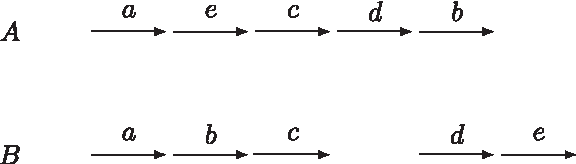
In this graphic representation of the genomes, each arrow represents a marker (from \documentclass{aastex}\usepackage{amsbsy}\usepackage{amsfonts}\usepackage{amssymb}\usepackage{bm}\usepackage{mathrsfs}\usepackage{pifont}\usepackage{stmaryrd}\usepackage{textcomp}\usepackage{portland, xspace}\usepackage{amsmath, amsxtra}\pagestyle{empty}\DeclareMathSizes{10}{9}{7}{6} \begin{document} $${\cal G} = \{ a , b , c , d , e \}$$ \end{document} ) with its corresponding orientation. Observe that genome A is composed of one, while genome B is composed of two linear chromosomes.

For each \documentclass{aastex}\usepackage{amsbsy}\usepackage{amsfonts}\usepackage{amssymb}\usepackage{bm}\usepackage{mathrsfs}\usepackage{pifont}\usepackage{stmaryrd}\usepackage{textcomp}\usepackage{portland, xspace}\usepackage{amsmath, amsxtra}\pagestyle{empty}\DeclareMathSizes{10}{9}{7}{6} \begin{document} $$g \in {\cal G}$$ \end{document} , we denote its two extremities by g^t (tail) and g^h (head), and we can represent an adjacency between two markers a and b in A by an unordered pair containing the extremities of a and b that are actually adjacent. For example, in genome A of Figure 1 the head of marker a is adjacent to the tail of marker e, thus we have the adjacency {a^h, e^t}, that we represent as a^he^t or e^ta^h for simplicity. Each end of a linear chromosome is called a telomere and is represented by the symbol ○. When the extremity of a marker is at one of the two ends of a linear chromosome, we have a pair containing the symbol ○. For example, again in genome A of Figure 1, the extremity a^t is at the end of a linear chromosome, thus we have the pair {○, a^t}, that we represent simply as ○a^t or a^t○. A genome A can be represented by the set V(A) containing its adjacencies (Bergeron et al., 2006).

The two genomes in Figure 1 can be represented by the following sets: \documentclass{aastex}\usepackage{amsbsy}\usepackage{amsfonts}\usepackage{amssymb}\usepackage{bm}\usepackage{mathrsfs}\usepackage{pifont}\usepackage{stmaryrd}\usepackage{textcomp}\usepackage{portland, xspace}\usepackage{amsmath, amsxtra}\pagestyle{empty}\DeclareMathSizes{10}{9}{7}{6}\begin{document} \begin{align*} V (A) = \{ \circ a^t , a^he^t , e^hc^t , c^hd^t , d^hb^t , b^h \circ \} \end{align*} \end{document}

and \documentclass{aastex}\usepackage{amsbsy}\usepackage{amsfonts}\usepackage{amssymb}\usepackage{bm}\usepackage{mathrsfs}\usepackage{pifont}\usepackage{stmaryrd}\usepackage{textcomp}\usepackage{portland, xspace}\usepackage{amsmath, amsxtra}\pagestyle{empty}\DeclareMathSizes{10}{9}{7}{6}\begin{document} \begin{align*} V (B) = \{ \circ a^t , a^hb^t , b^hc^t , c^h \circ , \circ d^t , d^he^t , e^h \circ \} . \end{align*} \end{document}

A double cut and join (DCJ) operation applied to a genome A is the operation that cuts two elements of V(A) and joins the separated extremities in a different way, creating two new adjacencies. For example, a DCJ acting on two adjacencies pq and rs would create either the adjacencies pr and qs, or the adjacencies ps and qr (this could correspond to an inversion, a reciprocal translocation between two linear chromosomes, a fusion of two circular chromosomes, or an excision of a circular chromosome). In the same way, a DCJ acting on two adjacencies pq and r○ would create either pr and q○, or p○ and qr (in this case, the operation could correspond to an inversion, a translocation, or a fusion of a circular and a linear chromosome). For the cases described so far, we can notice that for each pair of cuts there are two possibilities of joining.

There are two special cases of a DCJ operation, in which there is only one possibility of joining. The first is a DCJ acting on two adjacencies p○ and q○, that would create only one new adjacency pq (that could represent a circularization of one or a fusion of two linear chromosomes). Conversely, a DCJ can act on only one adjacency pq and create the two adjacencies p○ and q○ (representing a linearization of a circular or a fission of a linear chromosome).

Definition 1 (Bergeron et al., 2006)

Given two genomes A and B over the same set of markers \documentclass{aastex}\usepackage{amsbsy}\usepackage{amsfonts}\usepackage{amssymb}\usepackage{bm}\usepackage{mathrsfs}\usepackage{pifont}\usepackage{stmaryrd}\usepackage{textcomp}\usepackage{portland, xspace}\usepackage{amsmath, amsxtra}\pagestyle{empty}\DeclareMathSizes{10}{9}{7}{6} \begin{document} $${\cal G}$$ \end{document} (with the same content) and without duplications, the adjacency graph AG(A, B) is the graph with the following properties:
1. The set of vertices is \documentclass{aastex}\usepackage{amsbsy}\usepackage{amsfonts}\usepackage{amssymb}\usepackage{bm}\usepackage{mathrsfs}\usepackage{pifont}\usepackage{stmaryrd}\usepackage{textcomp}\usepackage{portland, xspace}\usepackage{amsmath, amsxtra}\pagestyle{empty}\DeclareMathSizes{10}{9}{7}{6} \begin{document} $$V = V_A \cup V_B$$ \end{document} where V_A has a vertex for each element in V(A) and V_B has a vertex for each element in V(B).

2. For each \documentclass{aastex}\usepackage{amsbsy}\usepackage{amsfonts}\usepackage{amssymb}\usepackage{bm}\usepackage{mathrsfs}\usepackage{pifont}\usepackage{stmaryrd}\usepackage{textcomp}\usepackage{portland, xspace}\usepackage{amsmath, amsxtra}\pagestyle{empty}\DeclareMathSizes{10}{9}{7}{6} \begin{document} $$g \in {\cal G}$$ \end{document} , we have one edge connecting the vertex in V_A and the vertex in V_B whose corresponding elements in V(A) and V(B) contain g^h and one edge connecting the vertex in V_A and the vertex in V_B whose corresponding elements in V(A) and V(B) contain g^t.

Although an element in V(A) can be identical to an element in V(B), the corresponding vertices in V_A and V_B are different and |V| = |V(A)| + |V(B)|. For simplicity, we will identify each vertex in V_A with the corresponding element in V(A) and each vertex in V_B with the corresponding element in V(B).

We know that AG(A, B) is bipartite with maximum degree equal to two (each extremity of a marker appears in one element in V(A) and in one element in V(B)). Consequently, AG(A, B) is a collection of cycles and paths, alternating vertices in V(A) and V(B). The length of a cycle or path is given by the number of edges it contains. A path is said to be balanced when it contains the same number of vertices in V(A) and in V(B), that is, when it contains an odd number of edges. Otherwise the path contains an even number of edges and is said to be unbalanced. We denote by AA-path an unbalanced path with more vertices in V(A), and by BB-path an unbalanced path with more vertices in V(B).

Each path starts and ends in vertices containing the symbol ○. Observe that both A and B have an even number of telomeres; thus, both V(A) and V(B) have an even number of adjacencies containing the symbol ○, and the number of balanced paths in AG(A, B) is even (Bergeron et al., 2006). An example of an adjacency graph is given in Figure 2.

FIG. 2.
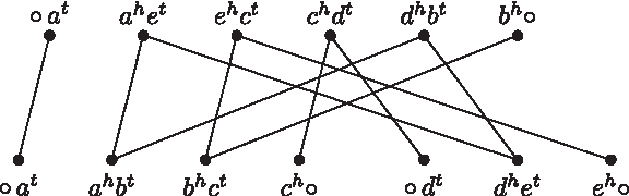
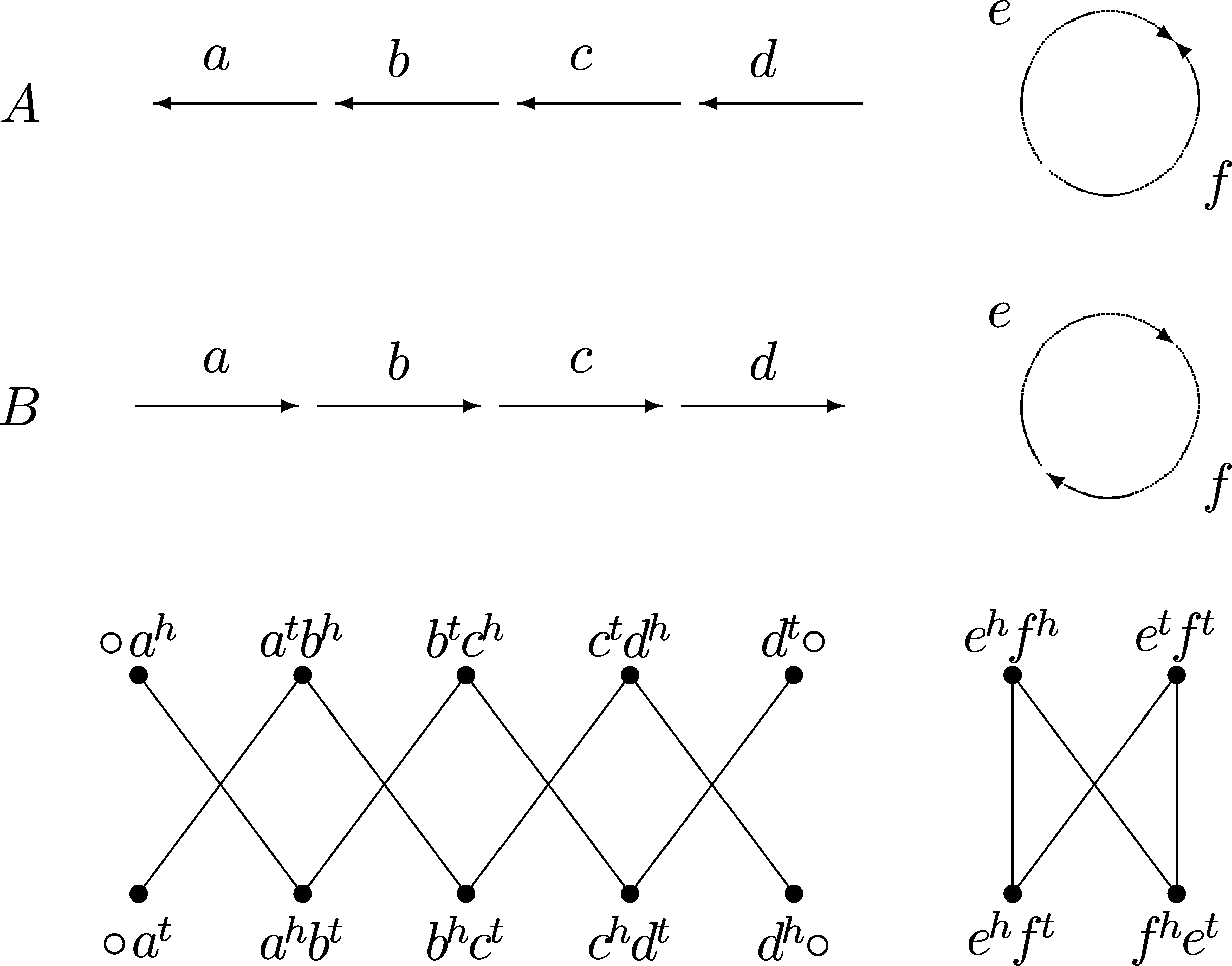
The adjacency graph for the linear genomes A and B from Figure 1, defined by the correponding sets of adjacencies V(A) = {○a^t, a^he^t, e^hc^t, c^hd^t, d^hb^t, b^h○} and V(B) = {○a^t, a^hb^t, b^hc^t, c^h○, ○d^t, d^he^t, e^h○}, contains one cycle, one unbalanced BB-path, and two balanced paths.

In the original notation proposed by Bergeron et al. (2006), balanced paths are called odd paths and unbalanced paths are called even paths, in reference to their lengths. However, the sorting by DCJ problem can be also studied with the help of the breakpoint graph (Fertin et al., 2009; Tannier et al., 2009), introduced by Hannenhalli and Pevzner (1995).

Given two genomes A and B, we denote by BG(A, B) the breakpoint graph of A and B. There is a duality between AG(A, B) and BG(A, B), so that AG(A, B) is the line graph of BG(A, B) and an odd path in AG(A, B) is an even path in BG(A, B) (analogously, an even path in AG(A, B) is an odd path in BG(A, B)). Calling these paths balanced and unbalanced is a general notation that is unambiguous, independently of the adopted graph. Moreover, this notation has a meaning with respect to the fact that in balanced paths the genomes are equally represented, while in unbalanced paths one genome is more represented than the other.

The DCJ distance between two genomes A and B, denoted by d(A, B), can be easily computed:

Theorem 1 (Bergeron et al., 2006)

Given two genomes A and B over the same set of markers \documentclass{aastex}\usepackage{amsbsy}\usepackage{amsfonts}\usepackage{amssymb}\usepackage{bm}\usepackage{mathrsfs}\usepackage{pifont}\usepackage{stmaryrd}\usepackage{textcomp}\usepackage{portland, xspace}\usepackage{amsmath, amsxtra}\pagestyle{empty}\DeclareMathSizes{10}{9}{7}{6} \begin{document} $${\cal G}$$ \end{document} and without duplications, the DCJ distance between A and B is given by \documentclass{aastex}\usepackage{amsbsy}\usepackage{amsfonts}\usepackage{amssymb}\usepackage{bm}\usepackage{mathrsfs}\usepackage{pifont}\usepackage{stmaryrd}\usepackage{textcomp}\usepackage{portland, xspace}\usepackage{amsmath, amsxtra}\pagestyle{empty}\DeclareMathSizes{10}{9}{7}{6}\begin{document} \begin{align} d (A , B) = n - c - \frac {b} {2} \end{align} \end{document}

where n is the number of markers in \documentclass{aastex}\usepackage{amsbsy}\usepackage{amsfonts}\usepackage{amssymb}\usepackage{bm}\usepackage{mathrsfs}\usepackage{pifont}\usepackage{stmaryrd}\usepackage{textcomp}\usepackage{portland, xspace}\usepackage{amsmath, amsxtra}\pagestyle{empty}\DeclareMathSizes{10}{9}{7}{6} \begin{document} $${\cal G}$$ \end{document} , c and b are respectively the number of cycles and balanced paths in AG(A, B).

An optimal DCJ operation is a DCJ operation that decreases the DCJ distance by one. Bergeron et al. (2006) observed that an optimal DCJ operation either increases the number of cycles by one or the number of balanced paths by two and proposed a simple greedy algorithm to find one solution to the sorting by DCJ problem, that is, one optimal sequence of DCJ operations to sort A into B.

3. Sorting Components Separately

Although an optimal DCJ sequence sorting a genome A into a genome B can be obtained easily (Bergeron et al., 2006), there are several different optimal sorting sequences, and in this study, we approach the problem of characterizing and counting these optimal solutions. We want to analyze the space of solutions sorting A into B; thus, we consider only operations acting on genome A, or, in other words, acting on vertices of V(A). We adopt the shorter notation A-vertex to refer to a vertex in V(A).

In this section, we focus on DCJ sequences that can be obtained by sorting separately the components of the adjacency graph of two genomes.

Proposition 1

For any pair of A-vertices belonging to the same component of AG(A, B), there is one, and only one optimal DCJ operation. This is also true for any single A-vertex belonging to an unbalanced BB-path of AG(A, B).

Proof

For each pair of A-vertices, such that at most, one contains the symbol ○, we know that there are two different DCJ operations. When the vertices belong to the same component C, one of the two operations simply inverts a segment, not changing the structure of C, and therefore cannot be optimal. The second operation would be an optimal DCJ operation that splits C into a cycle and a smaller component of the same type as C, increasing the number of cycles. This includes all pairs of vertices in cycles, balanced paths and BB-paths, and all pairs of vertices in AA-paths excluding the case where the two vertices contain the symbol ○.

For the two special cases, when both vertices contain the symbol ○ or when a DCJ operation is applied on a single adjacency, there is only one way of joining, thus at most one optimal DCJ operation exists. In the first case, the two vertices can be in the same component only if the component is an unbalanced AA-path. This DCJ operation would close the AA-path into a cycle and is optimal. In the second case, when the DCJ operation is applied on one single adjacency of a component, the operation is optimal (creates two balanced paths) only when the component is a BB-path. ▪

Proposition 2

Given two genomes A and B, any component of AG(A, B) can be sorted separately with only optimal DCJ operations.

Proof

This is a direct consequence of Proposition 1. ▪

Let C be a component in AG(A, B). Due to Proposition 2, we can define as d(C) the DCJ distance of C, that is the number of DCJ operations required to sort C separately. In the same way, we denote by ∥C∥ the number of optimal DCJ sequences that sort C separately.

We know that a component in AG(A, B) is either an even cycle, a balanced path, or an unbalanced path. Let EC_2ℓ+2 be an even cycle with 2ℓ + 2 edges and let BP_2ℓ+1 be a balanced and UP_2ℓ be an unbalanced path with respectively 2ℓ + 1 and 2ℓ edges. We call small components the paths and cycles of AG(A, B) with two vertices (BP₁ and EC₂) whose distance is zero; the other components are big components. Observe that any unbalanced path is a big component.

Theorem 2

For any integer \documentclass{aastex}\usepackage{amsbsy}\usepackage{amsfonts}\usepackage{amssymb}\usepackage{bm}\usepackage{mathrsfs}\usepackage{pifont}\usepackage{stmaryrd}\usepackage{textcomp}\usepackage{portland, xspace}\usepackage{amsmath, amsxtra}\pagestyle{empty}\DeclareMathSizes{10}{9}{7}{6} \begin{document} $$\ell \in \{ 1 , 2 , 3 , \ldots \}$$ \end{document} , we have d(UP_2ℓ) = d(BP_2ℓ+1) = d(EC_2ℓ+2) = ℓ and ∥UP_2ℓ∥ = ∥BP_2ℓ+1∥ = ∥EC_2ℓ+2∥.

Proof

In order to sort a cycle of length 2ℓ + 2, we need to split it into ℓ + 1 cycles of length 2. Each DCJ operation creates one new cycle, thus ℓ operations are required or, in other words, d(EC_2ℓ+2) = ℓ.

A balanced path with 2ℓ + 1 edges could be transformed into a cycle with 2ℓ + 2 edges by connecting the two ends of the path (this respects the alternation between vertices of V(A) and V(B)). Each sequence sorting the cycle would correspond to a sequence sorting the original balanced path, thus d(BP_2ℓ+1) = d(EC_2ℓ+2) = ℓ and ∥BP_2ℓ+1∥ = ∥EC_2ℓ+2∥. Analogously, an unbalanced path with 2ℓ edges could be transformed into a cycle with 2ℓ + 2 edges by the insertion of an “empty chromosome” vertex on the genome that is under-represented in the path. The two ends of the unbalanced path should then be connected to the new vertex (this also respects the alternation between vertices of V(A) and V(B)) and the new vertex can also be used in optimal DCJ operations within the unbalanced path. Again, each sequence sorting the cycle would correspond to a sequence sorting the original unbalanced path, thus d(UP_2ℓ) = d(EC_2ℓ+2) = ℓ and ∥UP_2ℓ∥ = ∥EC_2ℓ+2∥. ▪

An example for the case UP₂, BP₃ and EC₄ is given in Figure 3.

FIG. 3.
Linking telomeres in the paths of the adjacency graph. We can see here that the structures of an EC₄, a BP₃, and an UP₂ are identical; therefore, these components have the same DCJ distance and the same number of sorting sequences.

Let C₁ and C₂ be two big components of AG(A, B), with d(C₁) = ℓ₁ and d(C₂) = ℓ₂. Moreover, let s₁ be a DCJ sorting sequence of length ℓ₁ sorting C₁ and let s₂ be a DCJ sorting sequence of length ℓ₂ sorting C₂. We can obtain a set of sequences sorting C₁ and C₂ with the shuffle product of s₁ and s₂, denoted by s₁ ⨂ s₂, that corresponds to all possible ways of shuffling s₁ with s₂, such that s₁ and s₂ are subsequences of all resulting sequences. The number of sequences in s₁ ⨂ s₂ is given by the binomial coefficient \documentclass{aastex}\usepackage{amsbsy}\usepackage{amsfonts}\usepackage{amssymb}\usepackage{bm}\usepackage{mathrsfs}\usepackage{pifont}\usepackage{stmaryrd}\usepackage{textcomp}\usepackage{portland, xspace}\usepackage{amsmath, amsxtra}\pagestyle{empty}\DeclareMathSizes{10}{9}{7}{6} \begin{document} $${\ell_1 + \ell_2} \choose{\ell_1 , \ell_2}$$ \end{document} .

For example, if s₁ = ρ₁ρ₂ and s₂ = θ₁θ₂, then s₁ ⨂ s₂ is composed of the six sequences ρ₁ρ₂θ₁θ₂, ρ₁θ₁ρ₂θ₂, ρ₁θ₁θ₂ρ₂, θ₁ρ₁ρ₂θ₂, θ₁ρ₁θ₂ρ₂ and θ₁θ₂ρ₁ρ₂, and indeed \documentclass{aastex}\usepackage{amsbsy}\usepackage{amsfonts}\usepackage{amssymb}\usepackage{bm}\usepackage{mathrsfs}\usepackage{pifont}\usepackage{stmaryrd}\usepackage{textcomp}\usepackage{portland, xspace}\usepackage{amsmath, amsxtra}\pagestyle{empty}\DeclareMathSizes{10}{9}{7}{6} \begin{document} $$\big( {4 \atop 2 , 2} \big) = \frac {4!} {2!2!} = 6$$ \end{document} .

Observe that the operation ⨂ is commutative, that is, s₁ ⨂ s₂ = s₂ ⨂ s₁, and associative, that is, (s₁ ⨂ s₂) ⨂ s₃ = s₁ ⨂ (s₂ ⨂ s₃). In general, the number of ways of shuffling k sequences whose lengths are \documentclass{aastex}\usepackage{amsbsy}\usepackage{amsfonts}\usepackage{amssymb}\usepackage{bm}\usepackage{mathrsfs}\usepackage{pifont}\usepackage{stmaryrd}\usepackage{textcomp}\usepackage{portland, xspace}\usepackage{amsmath, amsxtra}\pagestyle{empty}\DeclareMathSizes{10}{9}{7}{6} \begin{document} $$\ell_1 , \ell_2 , \ldots , \ell_k$$ \end{document} , respectively, corresponds to the multinomial coefficient: \documentclass{aastex}\usepackage{amsbsy}\usepackage{amsfonts}\usepackage{amssymb}\usepackage{bm}\usepackage{mathrsfs}\usepackage{pifont}\usepackage{stmaryrd}\usepackage{textcomp}\usepackage{portland, xspace}\usepackage{amsmath, amsxtra}\pagestyle{empty}\DeclareMathSizes{10}{9}{7}{6}\begin{document} \begin{align} {\ell_1 + \ell_2 + \ldots + \ell_k \choose \ell_1 , \ell_2 , \ldots , \ell_k} = \frac {(\ell_1 + \ell_2 + \ldots + \ell_k)!} {\ell_1! \ell_2! \ldots \ell_k!}. \end{align} \end{document}

Now let S₁ be the set of all sequences sorting C₁ and S₂ be the set of all sequences sorting C₂. We can obtain all sequences sorting C₁ and C₂ by shuffling each sequence in S₁ with each sequence in S₂. For example, if S₁ = {s₁₁, s₁₂, s₁₃} and S₂ = {s₂₁}, then the result would be {s₁₁ ⨂ s₂₁, s₁₂ ⨂ s₂₁, s₁₃ ⨂ s₂₁}. We denote this by S₁ ⨂ S₂, or simply by C₁ ⨂ C₂. Observe that the operation ⨂ applied to sets is also commutative (C₁ ⨂ C₂ = C₂ ⨂ C₁) and associative ((C₁ ⨂ C₂) ⨂ C₃ = C₁ ⨂ (C₂ ⨂ C₃)).

If \documentclass{aastex}\usepackage{amsbsy}\usepackage{amsfonts}\usepackage{amssymb}\usepackage{bm}\usepackage{mathrsfs}\usepackage{pifont}\usepackage{stmaryrd}\usepackage{textcomp}\usepackage{portland, xspace}\usepackage{amsmath, amsxtra}\pagestyle{empty}\DeclareMathSizes{10}{9}{7}{6} \begin{document} $$C_1 , C_2 , \ldots C_k$$ \end{document} are the big components in AG(A, B) and \documentclass{aastex}\usepackage{amsbsy}\usepackage{amsfonts}\usepackage{amssymb}\usepackage{bm}\usepackage{mathrsfs}\usepackage{pifont}\usepackage{stmaryrd}\usepackage{textcomp}\usepackage{portland, xspace}\usepackage{amsmath, amsxtra}\pagestyle{empty}\DeclareMathSizes{10}{9}{7}{6} \begin{document} $$\ell_1 , \ell_2 , \ldots , \ell_k$$ \end{document} are their respective DCJ distances, then the number of sequences obtained by shuffling sequences sorting \documentclass{aastex}\usepackage{amsbsy}\usepackage{amsfonts}\usepackage{amssymb}\usepackage{bm}\usepackage{mathrsfs}\usepackage{pifont}\usepackage{stmaryrd}\usepackage{textcomp}\usepackage{portland, xspace}\usepackage{amsmath, amsxtra}\pagestyle{empty}\DeclareMathSizes{10}{9}{7}{6} \begin{document} $$C_1 , C_2 , \ldots , C_k$$ \end{document} separately can be given by the formula: \documentclass{aastex}\usepackage{amsbsy}\usepackage{amsfonts}\usepackage{amssymb}\usepackage{bm}\usepackage{mathrsfs}\usepackage{pifont}\usepackage{stmaryrd}\usepackage{textcomp}\usepackage{portland, xspace}\usepackage{amsmath, amsxtra}\pagestyle{empty}\DeclareMathSizes{10}{9}{7}{6}\begin{document} \begin{align} \mid C_1 \otimes C_2 \otimes \ldots \otimes C_k \mid = \mid \mid C_1 \mid \mid \times \mid \mid C_2 \mid \mid \times \ldots \times \mid \mid C_k \mid \mid \times \frac {(\ell_1 + \ell_2 + \ldots + \ell_k)!} {\ell_1! \ell_2! \ldots \ell_k!} \end{align} \end{document}

Theorem 3

The number of sequences sorting a big cycle EC_2ℓ+2 (whose distance is ℓ ≥ 1) is given by ∥EC_2ℓ+2∥ = (ℓ + 1)^ℓ−1.

Proof

From Proposition 1 we know that, for each pair of A-vertices, the cycle can be broken in only one way. If the cycle has v = ℓ + 1 A-vertices, it has 2v vertices and 2v edges. The result of the break for each pair of vertices are two cycles as follows (each pair of cycles can be obtained in v different ways):
one of size 2 (v′ = 1; ℓ′ = 0) and one of size 2v − 2 (v′ = v − 1; ℓ′ = ℓ − 1);

one of size 4 (v′ = 2; ℓ′ = 1) and one of size 2v − 4 (v′ = v − 2; ℓ′ = ℓ − 2);

one of size 6 (v′ = 3; ℓ′ = 2) and one of size 2v − 6 (v′ = v − 3; ℓ′ = ℓ − 3);

\documentclass{aastex}\usepackage{amsbsy}\usepackage{amsfonts}\usepackage{amssymb}\usepackage{bm}\usepackage{mathrsfs}\usepackage{pifont}\usepackage{stmaryrd}\usepackage{textcomp}\usepackage{portland, xspace}\usepackage{amsmath, amsxtra}\pagestyle{empty}\DeclareMathSizes{10}{9}{7}{6} \begin{document} $$\ldots$$ \end{document}

one of size 2i (v′ = i; ℓ′ = i − 1) and one of size 2(v − i) (v′ = v − i; ℓ′ = ℓ − i).

Thus, the number of sorting sequences can be computed by the following recurrence formula on v: \documentclass{aastex}\usepackage{amsbsy}\usepackage{amsfonts}\usepackage{amssymb}\usepackage{bm}\usepackage{mathrsfs}\usepackage{pifont}\usepackage{stmaryrd}\usepackage{textcomp}\usepackage{portland, xspace}\usepackage{amsmath, amsxtra}\pagestyle{empty}\DeclareMathSizes{10}{9}{7}{6}\begin{document} \begin{align} T (1) & = 1 \\ T (v) & = \mid \mid EC_{2v} \mid \mid \ = \ \frac {v} {2} \sum_{i = 1}^{v - 1} \mid EC_{2i} \otimes EC_{2(v - i)} \mid. \end{align} \end{document}

We know that \documentclass{aastex}\usepackage{amsbsy}\usepackage{amsfonts}\usepackage{amssymb}\usepackage{bm}\usepackage{mathrsfs}\usepackage{pifont}\usepackage{stmaryrd}\usepackage{textcomp}\usepackage{portland, xspace}\usepackage{amsmath, amsxtra}\pagestyle{empty}\DeclareMathSizes{10}{9}{7}{6} \begin{document} $$\mid EC_{2i} \otimes EC_{2 (v - i)} \mid = \mid \mid EC_{2i} \mid \mid \times \mid \mid EC_{2 (v - i)} \mid \mid \times {v - 2 \choose i - 1 , v - i - 1} = T (i) \times T (v - i) \times {v - 2 \choose i - 1}$$ \end{document} . Thus, we have \documentclass{aastex}\usepackage{amsbsy}\usepackage{amsfonts}\usepackage{amssymb}\usepackage{bm}\usepackage{mathrsfs}\usepackage{pifont}\usepackage{stmaryrd}\usepackage{textcomp}\usepackage{portland, xspace}\usepackage{amsmath, amsxtra}\pagestyle{empty}\DeclareMathSizes{10}{9}{7}{6} \begin{document} $$T (v) = \frac {v} {2} \sum\nolimits_{i = 1}^{v - 1} {v - 2 \choose i - 1} \times T (i) \times T (v - i)$$ \end{document} , or, alternatively \documentclass{aastex}\usepackage{amsbsy}\usepackage{amsfonts}\usepackage{amssymb}\usepackage{bm}\usepackage{mathrsfs}\usepackage{pifont}\usepackage{stmaryrd}\usepackage{textcomp}\usepackage{portland, xspace}\usepackage{amsmath, amsxtra}\pagestyle{empty}\DeclareMathSizes{10}{9}{7}{6} \begin{document} $$T (v) = \frac {v} {2} \sum\nolimits_{k = 0}^{v - 2} {v - 2 \choose k} \times T (k + 1) \times T (v - k - 1)$$ \end{document} , which is also equivalent to \documentclass{aastex}\usepackage{amsbsy}\usepackage{amsfonts}\usepackage{amssymb}\usepackage{bm}\usepackage{mathrsfs}\usepackage{pifont}\usepackage{stmaryrd}\usepackage{textcomp}\usepackage{portland, xspace}\usepackage{amsmath, amsxtra}\pagestyle{empty}\DeclareMathSizes{10}{9}{7}{6}\begin{document} \begin{align} T (v) = \sum_{k = 0}^{v - 2} {v - 2 \choose k} \times (v - k - 1) \times T (v - k - 1) \times T (k + 1). \end{align} \end{document}

This last recurrence formula is identical to the recurrence formula presented by Zeilberger (2010) for counting labeled trees and results in v^v⁻². Since we have ℓ = v − 1, we get T(v) = (ℓ + 1)^ℓ−1. ▪

Observe that the number of sequences sorting a cycle, given by Theorem 3, corresponds to the number of other objects in combinatorics, such as parking functions. The bijection between these objects and the DCJ sorting sequences has been demonstrated in Ouangraoua and Bergeron (2010).

In order to summarize the previous results, the DCJ distance and the number of sequences sorting the different types of big components are shown in Table 1.

Table 1.
Number of DCJ Sequences Sorting Each Type of Component Separately

Unbalanced paths Balanced paths Even cycles Sequence length Number of sequences

UP ₂ BP ₃ EC ₄ 1 1

UP ₄ BP ₅ EC ₆ 2 3

UP ₆ BP ₇ EC ₈ 3 16

UP ₈ BP ₉ EC ₁₀ 4 125

UP ₁₀ BP ₁₁ EC ₁₂ 5 1296

UP ₁₂ BP ₁₃ EC ₁₄ 6 16807

\documentclass{aastex}\usepackage{amsbsy}\usepackage{amsfonts}\usepackage{amssymb}\usepackage{bm}\usepackage{mathrsfs}\usepackage{pifont}\usepackage{stmaryrd}\usepackage{textcomp}\usepackage{portland, xspace}\usepackage{amsmath, amsxtra}\pagestyle{empty}\DeclareMathSizes{10}{9}{7}{6} \begin{document} $$\vdots$$ \end{document} \documentclass{aastex}\usepackage{amsbsy}\usepackage{amsfonts}\usepackage{amssymb}\usepackage{bm}\usepackage{mathrsfs}\usepackage{pifont}\usepackage{stmaryrd}\usepackage{textcomp}\usepackage{portland, xspace}\usepackage{amsmath, amsxtra}\pagestyle{empty}\DeclareMathSizes{10}{9}{7}{6} \begin{document} $$\vdots$$ \end{document} \documentclass{aastex}\usepackage{amsbsy}\usepackage{amsfonts}\usepackage{amssymb}\usepackage{bm}\usepackage{mathrsfs}\usepackage{pifont}\usepackage{stmaryrd}\usepackage{textcomp}\usepackage{portland, xspace}\usepackage{amsmath, amsxtra}\pagestyle{empty}\DeclareMathSizes{10}{9}{7}{6} \begin{document} $$\vdots$$ \end{document} \documentclass{aastex}\usepackage{amsbsy}\usepackage{amsfonts}\usepackage{amssymb}\usepackage{bm}\usepackage{mathrsfs}\usepackage{pifont}\usepackage{stmaryrd}\usepackage{textcomp}\usepackage{portland, xspace}\usepackage{amsmath, amsxtra}\pagestyle{empty}\DeclareMathSizes{10}{9}{7}{6} \begin{document} $$\vdots$$ \end{document} \documentclass{aastex}\usepackage{amsbsy}\usepackage{amsfonts}\usepackage{amssymb}\usepackage{bm}\usepackage{mathrsfs}\usepackage{pifont}\usepackage{stmaryrd}\usepackage{textcomp}\usepackage{portland, xspace}\usepackage{amsmath, amsxtra}\pagestyle{empty}\DeclareMathSizes{10}{9}{7}{6} \begin{document} $$\vdots$$ \end{document}

UP _2ℓ BP _2ℓ+1 EC _2ℓ+2 ℓ (ℓ + 1)^ℓ−1

Theorem 4

The number of solutions sorting AG(A, B) obtained by sorting each component separately is \documentclass{aastex}\usepackage{amsbsy}\usepackage{amsfonts}\usepackage{amssymb}\usepackage{bm}\usepackage{mathrsfs}\usepackage{pifont}\usepackage{stmaryrd}\usepackage{textcomp}\usepackage{portland, xspace}\usepackage{amsmath, amsxtra}\pagestyle{empty}\DeclareMathSizes{10}{9}{7}{6}\begin{document} \begin{align} S_{sep} \ = \ \mid C_1 \otimes C_2 \otimes \ldots \otimes C_k \mid \ = \ \frac {(\ell_1 + \ell_2 + \ldots + \ell_k)!} {\ell_1! \ell_2! \ldots \ell_k!} \times \prod_{i = 1}^k (\ell_i + 1)^{\ell_i - 1} \end{align} \end{document}

where \documentclass{aastex}\usepackage{amsbsy}\usepackage{amsfonts}\usepackage{amssymb}\usepackage{bm}\usepackage{mathrsfs}\usepackage{pifont}\usepackage{stmaryrd}\usepackage{textcomp}\usepackage{portland, xspace}\usepackage{amsmath, amsxtra}\pagestyle{empty}\DeclareMathSizes{10}{9}{7}{6} \begin{document} $$C_1 , C_2 , \ldots , C_k$$ \end{document} are the big components of AG(A, B) and \documentclass{aastex}\usepackage{amsbsy}\usepackage{amsfonts}\usepackage{amssymb}\usepackage{bm}\usepackage{mathrsfs}\usepackage{pifont}\usepackage{stmaryrd}\usepackage{textcomp}\usepackage{portland, xspace}\usepackage{amsmath, amsxtra}\pagestyle{empty}\DeclareMathSizes{10}{9}{7}{6} \begin{document} $$\ell_1 , \ell_2 , \ldots , \ell_k$$ \end{document} are their respective DCJ distances.

Proof

We know that the number of solutions obtained by shuffling the sequences sorting the components separately is given by the multinomial coefficient multiplied by the number of sequences sorting each component, the latter being given by Theorems 2 and 3. ▪

4. Recombining Unbalanced Paths

The formula given by Theorem 4 does not correspond to the total number of solutions for a general instance of the problem, due to the recombination of unbalanced paths. More precisely, a pair composed of one AA-path and one BB-path, called a pair of alternate unbalanced paths, can be recombined into two balanced paths and this is an optimal DCJ operation. Figure 4 shows two examples of such recombinations.

FIG. 4.
Here we represent two of many ways of recombining a pair of alternate unbalanced paths into a pair of balanced paths.

Proposition 3

Given two genomes A and B, a DCJ operation acting on two A-vertices belonging to two different components of AG(A, B) is optimal, if and only if the two components are alternate unbalanced paths.

Proof

Recall that an optimal DCJ operation either increases the number of cycles by one or the number of balanced paths by two (Bergeron et al., 2006). We need to examine all possible DCJ operations acting on two different components C₁ and C₂ of AG(A, B). If C₁ is a cycle, then the result is one single component that is of the same type as C₂. Thus, the cycle C₁ disappears and the number of cycles in the graph is reduced. If C₁ and C₂ are balanced paths, then the result is either one unbalanced path, or two unbalanced, or two balanced paths. In the first and the second case, the number of balanced paths is reduced by two and in the third case it remains unchanged. If C₁ is a balanced and C₂ is an unbalanced path, then the result is either one balanced path, or one balanced and one unbalanced path. In both cases, the number of balanced paths remains unchanged. And the same happens if C₁ and C₂ are unbalanced paths that do not form an alternate pair. In this case, the result is either one, or two unbalanced paths. Note that all operations enumerated so far are not optimal. The last possibility is when C₁ and C₂ are a pair of alternate unbalanced paths. In this case, any operation acting on one A-vertex of C₁ and one A-vertex of C₂ results in a pair of balanced paths (Fig. 4) and is an optimal DCJ operation. ▪

Proposition 3 guarantees that, if AG(A, B) does not contain any pair of alternate unbalanced paths, the components of AG(A, B) can only be sorted separately.

Corollary 1

Given two genomes A and B, such that AG(A, B) does not contain a pair of alternate unbalanced paths, the formula of Theorem 4 gives the exact number of sorting sequences that transform A into B.

However, although the unbalanced paths can be recombined, they can also be sorted separately. Thus, we have:

Corollary 2

The formula given in Theorem 4 is a lower bound to the number of DCJ sorting sequences for any instance of the problem.

A pair of alternate unbalanced paths can be recombined into two balanced paths at any time and in several different ways, since each one of the unbalanced paths can be reduced before the recombination, by the extraction of cycles. Moreover, two or more different pairs of alternate unbalanced paths can be recombined simultaneously.

Observe, however, that after one recombination we have a pair of balanced paths, so in any optimal sorting sequence an unbalanced path can participate in at most one recombination. Once a recombination occurs, the resulting balanced paths are then sorted separately.

It is possible to design a procedure to count the number of sequences recombining a pair of alternate unbalanced paths, and then combine this with a method to determine all possible simultaneous recombinations to compute the total number of DCJ sequences sorting one genome into another. This is what we do in the following two subsections.

4.1. Recombining one pair of alternate unbalanced paths

First we will analyze how to compute the ways of recombining a single pair of alternate unbalanced paths P_A and P_B, as shown in Figure 5.

FIG. 5.
A single pair of alternate unbalanced paths P_A and P_B.

Observe that for each A-vertex in P_A and each A-vertex in P_B, there are two optimal DCJ operations:

Proposition 4

The two different DCJ operations acting on one A-vertex in an AA-path and one A-vertex in a BB-path are optimal.

Proof

This can be verified by simple enumeration, as illustrated in Figure 6. ▪

FIG. 6.
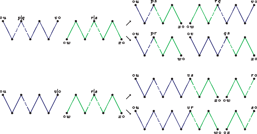
The two ways of recombining a pair of alternate unbalanced paths using vertices pq and rs and the two ways of recombining a pair of alternate unbalanced paths using vertices v○ and rs.

One way of counting the number of DCJ sequences recombining an AA-path P_A and a BB-path P_B is to link them together into a cycle. In the first way, the first telomere in P_A is linked with the second telomere in P_B and the second telomere in P_A with the first telomere in P_B. We denote this cycle by c₁(P_A, P_B). In fact, there are two ways of linking the paths together. The other way would be to link the first telomere in P_A with the first telomere in P_B and the second telomere in P_A with the second telomere in P_B, resulting in a cycle denoted by c₂(P_A, P_B). If d(P_A) = ℓ_A and d(P_B) = ℓ_B, then both c₁(P_A, P_B) and c₂(P_A, P_B) have DCJ distance equal to ℓ_A + ℓ_B. Figure 7 shows the two ways of linking a pair of unbalanced paths.

FIG. 7.
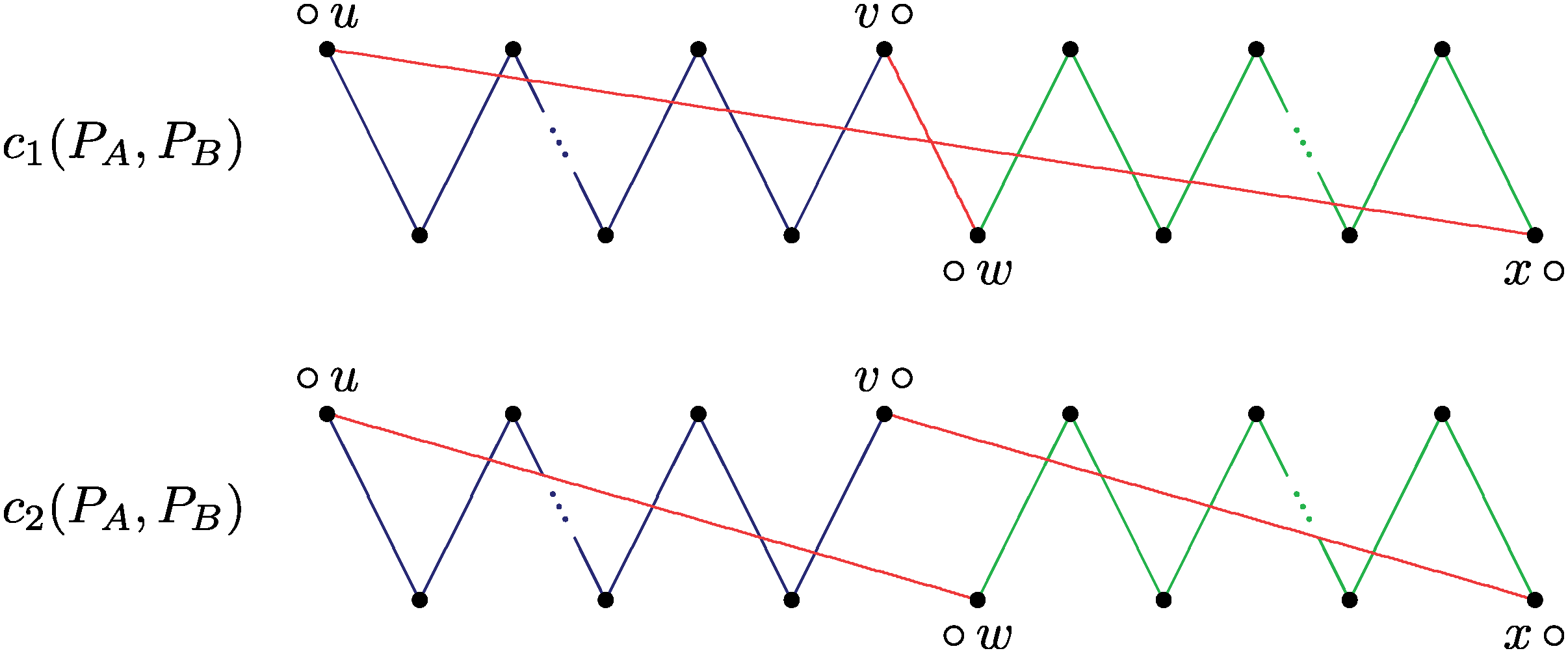
The two ways of linking an AA-path and a BB-path together into a cycle.

Observe that all vertices in P_A and all vertices in P_B are also present in both c₁(P_A, P_B) and c₂(P_A, P_B).

Proposition 5

Each optimal DCJ operation acting on one A-vertex in an AA-path P_A and one A-vertex in a BB-path P_B corresponds either to one optimal DCJ operation splitting c₁(P_A, P_B) or to one optimal DCJ operation splitting c₂(P_A, P_B).

Proof

Let pq be an A-vertex in P_A and rs be an A-vertex in P_B. Both vertices pq and rs are present in both cycles c₁(P_A, P_B) and c₂(P_A, P_B). There are two optimal DCJ operations acting on pq and rs, one creates the vertices pr and qs and the other creates the vertices ps and qr. Without loss of generality, suppose that the first possibility would correspond to a splitting in c₁(P_A, P_B). Then since P_B would be inversed in c₂(P_A, P_B) with respect to c₁(P_A, P_B), the second would correspond to a splitting in c₂(P_A, P_B). A similar analysis can be done to the case when v○ is an A-vertex in P_A and rs is an A-vertex in P_B. ▪

Proposition 5 establishes a relation between an operation recombining two unbalanced paths P_A and P_B and an operation splitting a cycle whose distance is the sum of the distances of P_A and P_B. A consequence of this fact is that any optimal sequence of operations that sorts P_A and P_B and contains a recombining operation would correspond to an optimal sequence of operations sorting a cycle whose distance is the sum of the distances of P_A and P_B:

Proposition 6

Each optimal DCJ sequence recombining an AA-path P_A and a BB-path P_B corresponds either to one optimal DCJ sequence sorting c₁(P_A, P_B) or to one optimal DCJ sequence sorting c₂(P_A, P_B).

Corollary 3

The number of sorting sequences recombining an AA-path P_A and a BB-path P_B whose DCJ distances are, respectively, ℓ_A and ℓ_B is bounded by 2 × (ℓ_A + ℓ_B + 1)ℓ_A+ℓ_B⁻¹.

Not all the sequences sorting c₁(P_A, P_B) and c₂(P_A, P_B) correspond to recombining DCJ sequences. Look at the examples in Figure 8.

FIG. 8.
The first operation sorting c₁(P_A, P_B) does not necessarily recombine. Observe that in (1) the original paths would be clearly sorted separately. In (2) the AA-path is reduced, but the recombination can still occur in a subsequent step.

Observe that in Figure 8 (1), we create the vertex ○○. In this case, the original paths would be clearly sorted separately. On the other hand, an operation that actually recombines the two original paths would separate the vertices containing the symbols ○ and ○ in two different cycles without creating the vertex ○○, as we can see in Figure 9.

FIG. 9.
The first operation splits c₁(P_A, P_B) and separates the vertices ○ u and v○ in two different cycles, so that the vertex ○○ cannot be created in any subsequent step. In this case, the paths P_A and P_B are recombined.

Indeed, after the vertices that contain the symbols ○ and ○ are separated in two different cycles, we cannot create the vertex ○○ in any subsequent step. The separation does not need to happen in the first step. We can first apply some operations internal to the original paths, and obtain an intermediary state where the separation can still occur, as in Figure 8 (2). In this case, we have two cycles, but the vertices that contain the symbols ○ and ○ are still in the same cycle, so we can still create the vertex ○○.

Proposition 7

Only the solutions that create the vertex ○○ in some step do not recombine the original paths.

Counting sequences that create the vertex ○○. It is not very difficult to design a recurrence that, given an AA-path P_A and a BB-path P_B, counts the number of solutions that create the vertex ○○ in c₁(P_A, P_B) (or in c₂(P_A, P_B)).

First, we define some operations over a pair of integers [n, ℓ], where n ≥ 1 and ℓ ≥ 0 (usually n gives the number of sequences and ℓ the length of the sequences):
[n₁, ℓ] + [n₂, ℓ] = [n₁ + n₂, ℓ] (the addition is only defined when the second value is the same for both pairs);

[n₁, ℓ] − [n₂, ℓ] = [n₁ − n₂, ℓ] (the subtraction is only defined when the second value is the same for both pairs and n₁ > n₂);

i × [n, ℓ] = [i × n, ℓ] (i ≥ 1 is an integer);

[n₁, ℓ₁] × [n₂, ℓ₂] = [n₁ × n₂, ℓ₁ + ℓ₂] (concatenating n₁ sequences of length ℓ₁ with n₂ sequences of length ℓ₂);

\documentclass{aastex}\usepackage{amsbsy}\usepackage{amsfonts}\usepackage{amssymb}\usepackage{bm}\usepackage{mathrsfs}\usepackage{pifont}\usepackage{stmaryrd}\usepackage{textcomp}\usepackage{portland, xspace}\usepackage{amsmath, amsxtra}\pagestyle{empty}\DeclareMathSizes{10}{9}{7}{6} \begin{document} $$[n_1 , \ell_1] \otimes [n_2 , \ell_2] = \left[n_1 \times n_2 \times \frac {(\ell_1 + \ell_2)!} {\ell_1! \ell_2!} , \ell_1 + \ell_2 \right]$$ \end{document} (shuffling n₁ sequences of length ℓ₁ with n₂ sequences of length ℓ₂).

Here we denote by \documentclass{aastex}\usepackage{amsbsy}\usepackage{amsfonts}\usepackage{amssymb}\usepackage{bm}\usepackage{mathrsfs}\usepackage{pifont}\usepackage{stmaryrd}\usepackage{textcomp}\usepackage{portland, xspace}\usepackage{amsmath, amsxtra}\pagestyle{empty}\DeclareMathSizes{10}{9}{7}{6} \begin{document} $${\cal S} (\ell) = [(\ell + 1)^{\ell - 1} , \ell]$$ \end{document} the pair of integers in which the first part, given by Theorem 3, is the number of solutions sorting EC_2ℓ+2, whose DCJ distance is ℓ.

Given an AA-path P_A and a BB-path P_B, the number of sequences sorting c₁(P_A, P_B) that create the vertex ○○ depends only on the DCJ distances d(P_A) = ℓ_A and d(P_B) = ℓ_B. We denote by \documentclass{aastex}\usepackage{amsbsy}\usepackage{amsfonts}\usepackage{amssymb}\usepackage{bm}\usepackage{mathrsfs}\usepackage{pifont}\usepackage{stmaryrd}\usepackage{textcomp}\usepackage{portland, xspace}\usepackage{amsmath, amsxtra}\pagestyle{empty}\DeclareMathSizes{10}{9}{7}{6} \begin{document} $${\cal W} (\ell_A , \ell_B) = [w (\ell_A , \ell_B) , \ell_A + \ell_B]$$ \end{document} the pair of integers in which w(ℓ_A, ℓ_B) is the number of sequences of length ℓ_A + ℓ_B that sort c₁(P_A, P_B) (or c₂(P_A, P_B)) without recombining P_A and P_B.

We need \documentclass{aastex}\usepackage{amsbsy}\usepackage{amsfonts}\usepackage{amssymb}\usepackage{bm}\usepackage{mathrsfs}\usepackage{pifont}\usepackage{stmaryrd}\usepackage{textcomp}\usepackage{portland, xspace}\usepackage{amsmath, amsxtra}\pagestyle{empty}\DeclareMathSizes{10}{9}{7}{6} \begin{document} $${\cal S} (\ell_A + \ell_B) \ {\rm and} \ {\cal W} (\ell_A , \ell_B)$$ \end{document} to compute \documentclass{aastex}\usepackage{amsbsy}\usepackage{amsfonts}\usepackage{amssymb}\usepackage{bm}\usepackage{mathrsfs}\usepackage{pifont}\usepackage{stmaryrd}\usepackage{textcomp}\usepackage{portland, xspace}\usepackage{amsmath, amsxtra}\pagestyle{empty}\DeclareMathSizes{10}{9}{7}{6} \begin{document} $${\cal R} (\ell_A , \ell_B) = [r (\ell_A , \ell_B) , \ell_A + \ell_B]$$ \end{document} , where r(ℓ_A, ℓ_B) is the number of sequences of length ℓ_A + ℓ_B that recombine an AA-path whose DCJ distance is ℓ_A with a BB-path whose DCJ distance is ℓ_B: \documentclass{aastex}\usepackage{amsbsy}\usepackage{amsfonts}\usepackage{amssymb}\usepackage{bm}\usepackage{mathrsfs}\usepackage{pifont}\usepackage{stmaryrd}\usepackage{textcomp}\usepackage{portland, xspace}\usepackage{amsmath, amsxtra}\pagestyle{empty}\DeclareMathSizes{10}{9}{7}{6}\begin{document} \begin{align} {\cal R} (\ell_A , \ell_B) = 2 ({\cal S} (\ell_A + \ell_B) - {\cal W} (\ell_A , \ell_B)). \end{align} \end{document}

The recurrence for computing \documentclass{aastex}\usepackage{amsbsy}\usepackage{amsfonts}\usepackage{amssymb}\usepackage{bm}\usepackage{mathrsfs}\usepackage{pifont}\usepackage{stmaryrd}\usepackage{textcomp}\usepackage{portland, xspace}\usepackage{amsmath, amsxtra}\pagestyle{empty}\DeclareMathSizes{10}{9}{7}{6} \begin{document} $${\cal W} (\ell_A , \ell_B)$$ \end{document} is given by the following: \documentclass{aastex}\usepackage{amsbsy}\usepackage{amsfonts}\usepackage{amssymb}\usepackage{bm}\usepackage{mathrsfs}\usepackage{pifont}\usepackage{stmaryrd}\usepackage{textcomp}\usepackage{portland, xspace}\usepackage{amsmath, amsxtra}\pagestyle{empty}\DeclareMathSizes{10}{9}{7}{6}\begin{document} \begin{align} {\cal W} (\ell_A , \ell_B) = [n , \ell_A + \ell_B] = [1 , 1] \times [n , \ell_A + \ell_B - 1] = [1 , 1] \times (X + Y + Z) \end{align} \end{document}

where the first part ([1, 1]) represents the first step and the second part (X + Y + Z = [n, ℓ_A + ℓ_B − 1]) considers all possible effects of the first step (all non-recombining steps):

\documentclass{aastex}\usepackage{amsbsy}\usepackage{amsfonts}\usepackage{amssymb}\usepackage{bm}\usepackage{mathrsfs}\usepackage{pifont}\usepackage{stmaryrd}\usepackage{textcomp}\usepackage{portland, xspace}\usepackage{amsmath, amsxtra}\pagestyle{empty}\DeclareMathSizes{10}{9}{7}{6} \begin{document} $$X = \sum\nolimits_{i = 1}^{\ell_A - 1} (i + 1) \times {\cal W} (i , \ell_B) \otimes {\cal S} (\ell_A - i - 1)$$ \end{document} (reduce the AA-path extracting a (2[ℓ_A − i − 1] + 2)-cycle)

\documentclass{aastex}\usepackage{amsbsy}\usepackage{amsfonts}\usepackage{amssymb}\usepackage{bm}\usepackage{mathrsfs}\usepackage{pifont}\usepackage{stmaryrd}\usepackage{textcomp}\usepackage{portland, xspace}\usepackage{amsmath, amsxtra}\pagestyle{empty}\DeclareMathSizes{10}{9}{7}{6} \begin{document} $$Y = \sum\nolimits_{i = 1}^{\ell_B - 1} i \times {\cal W} (\ell_A , i) \otimes {\cal S} (\ell_B - i - 1)$$ \end{document} (reduce the BB-path extracting a (2[ℓ_B − i − 1] + 2)-cycle)

\documentclass{aastex}\usepackage{amsbsy}\usepackage{amsfonts}\usepackage{amssymb}\usepackage{bm}\usepackage{mathrsfs}\usepackage{pifont}\usepackage{stmaryrd}\usepackage{textcomp}\usepackage{portland, xspace}\usepackage{amsmath, amsxtra}\pagestyle{empty}\DeclareMathSizes{10}{9}{7}{6} \begin{document} $$Z = {\cal S} (\ell_A - 1) \otimes {\cal S} (\ell_B)$$ \end{document} (separate the paths)

Observe that \documentclass{aastex}\usepackage{amsbsy}\usepackage{amsfonts}\usepackage{amssymb}\usepackage{bm}\usepackage{mathrsfs}\usepackage{pifont}\usepackage{stmaryrd}\usepackage{textcomp}\usepackage{portland, xspace}\usepackage{amsmath, amsxtra}\pagestyle{empty}\DeclareMathSizes{10}{9}{7}{6} \begin{document} $${\cal W} (1 , 1) = [1 , 1] \times ({\cal S} (0) \otimes {\cal S} (1)) = [1 , 1] \times ([1 , 0] \otimes [1 , 1]) = [1 , 1] \times [1 , 1] = [1 , 2]$$ \end{document} .

Complexity of computing the recurrence. In order to compute \documentclass{aastex}\usepackage{amsbsy}\usepackage{amsfonts}\usepackage{amssymb}\usepackage{bm}\usepackage{mathrsfs}\usepackage{pifont}\usepackage{stmaryrd}\usepackage{textcomp}\usepackage{portland, xspace}\usepackage{amsmath, amsxtra}\pagestyle{empty}\DeclareMathSizes{10}{9}{7}{6} \begin{document} $${\cal W} (\ell_A , \ell_B)$$ \end{document} by dynamic programming, we need to fill a matrix of size ℓ_B × ℓ_A. From the recurrence, we observe that an entry in line i and column j depends on all previous values in line i (that is, columns \documentclass{aastex}\usepackage{amsbsy}\usepackage{amsfonts}\usepackage{amssymb}\usepackage{bm}\usepackage{mathrsfs}\usepackage{pifont}\usepackage{stmaryrd}\usepackage{textcomp}\usepackage{portland, xspace}\usepackage{amsmath, amsxtra}\pagestyle{empty}\DeclareMathSizes{10}{9}{7}{6} \begin{document} $$1 , 2 , \ldots , j - 1$$ \end{document} of line i) and on all previous values in column j (that is, lines \documentclass{aastex}\usepackage{amsbsy}\usepackage{amsfonts}\usepackage{amssymb}\usepackage{bm}\usepackage{mathrsfs}\usepackage{pifont}\usepackage{stmaryrd}\usepackage{textcomp}\usepackage{portland, xspace}\usepackage{amsmath, amsxtra}\pagestyle{empty}\DeclareMathSizes{10}{9}{7}{6} \begin{document} $$1 , 2 , \ldots , i - 1$$ \end{document} of column j). Thus, the complexity is O(ℓ_Aℓ_B) space and O(ℓ_Aℓ_B(ℓ_A + ℓ_B)) time. These are also the complexities to compute \documentclass{aastex}\usepackage{amsbsy}\usepackage{amsfonts}\usepackage{amssymb}\usepackage{bm}\usepackage{mathrsfs}\usepackage{pifont}\usepackage{stmaryrd}\usepackage{textcomp}\usepackage{portland, xspace}\usepackage{amsmath, amsxtra}\pagestyle{empty}\DeclareMathSizes{10}{9}{7}{6} \begin{document} $${\cal R} (\ell_A , \ell_B)$$ \end{document} .

Counting sequences that recombine a pair of alternate unbalanced paths. We used the previous recurrence to count the recombining solutions for some pairs of alternate unbalanced paths with different DCJ distances. The results are given in Table 2.

Table 2.
Computing Sequences Recombining Alternate Unbalanced Paths

AA-path d = ℓ_A BB-path d = ℓ_B Non-recombining: \documentclass{aastex}\usepackage{amsbsy}\usepackage{amsfonts}\usepackage{amssymb}\usepackage{bm}\usepackage{mathrsfs}\usepackage{pifont}\usepackage{stmaryrd}\usepackage{textcomp}\usepackage{portland, xspace}\usepackage{amsmath, amsxtra}\pagestyle{empty}\DeclareMathSizes{10}{9}{7}{6} \begin{document} $${\cal W} (\ell_A , \ell_B)$$ \end{document} All recombining solutions: \documentclass{aastex}\usepackage{amsbsy}\usepackage{amsfonts}\usepackage{amssymb}\usepackage{bm}\usepackage{mathrsfs}\usepackage{pifont}\usepackage{stmaryrd}\usepackage{textcomp}\usepackage{portland, xspace}\usepackage{amsmath, amsxtra}\pagestyle{empty}\DeclareMathSizes{10}{9}{7}{6} \begin{document} $${\cal R} (\ell_A , \ell_B) = 2 ({\cal S} (\ell_A + \ell_B) - {\cal W} (\ell_A , \ell_B))$$ \end{document}

1 1 1 4

1 2 4 24

1 3 27 196

1 4 256 2, 080

1 5 3, 125 27, 364

1 6 46, 656 430, 976

1 7 823, 543 7, 918, 852

1 8 16, 777, 216 166, 445, 568

1 9 387, 420, 489 3, 941, 054, 404

2 1 4 24

2 2 21 208

2 3 176 2, 240

2 4 1, 995 29, 624

2 5 28, 344 467, 600

2 6 482, 825 8, 600, 288

2 7 9, 576, 160 180, 847, 680

2 8 216, 559, 287 4, 282, 776, 808

3 1 27 196

3 2 176 2, 240

3 3 1, 765 30, 084

3 4 23, 304 477, 680

3 5 378, 007 8, 809, 924

3 6 7, 238, 944 185, 522, 112

3 7 159, 444, 585 4, 397, 006, 212

Columns 3 and 4 should be given as pairs of integers [n, ℓ], but since ℓ = ℓ_A + ℓ_B for both columns, we only give the first value in each pair.

4.2. Computing all simultaneous recombinations

The computation of the number of all DCJ sorting sequences requires the values given by \documentclass{aastex}\usepackage{amsbsy}\usepackage{amsfonts}\usepackage{amssymb}\usepackage{bm}\usepackage{mathrsfs}\usepackage{pifont}\usepackage{stmaryrd}\usepackage{textcomp}\usepackage{portland, xspace}\usepackage{amsmath, amsxtra}\pagestyle{empty}\DeclareMathSizes{10}{9}{7}{6} \begin{document} $${\cal R} (\ell_A , \ell_B)$$ \end{document} for all pairs of integers ℓ_A and ℓ_B such that ℓ_A is the DCJ distance of an AA-path and ℓ_B is the DCJ distance of a BB-path in AG(A, B). Observe, however, that if \documentclass{aastex}\usepackage{amsbsy}\usepackage{amsfonts}\usepackage{amssymb}\usepackage{bm}\usepackage{mathrsfs}\usepackage{pifont}\usepackage{stmaryrd}\usepackage{textcomp}\usepackage{portland, xspace}\usepackage{amsmath, amsxtra}\pagestyle{empty}\DeclareMathSizes{10}{9}{7}{6} \begin{document} $$\ell_A^{max}$$ \end{document} is an upper bound to the DCJ distance of all AA-paths and \documentclass{aastex}\usepackage{amsbsy}\usepackage{amsfonts}\usepackage{amssymb}\usepackage{bm}\usepackage{mathrsfs}\usepackage{pifont}\usepackage{stmaryrd}\usepackage{textcomp}\usepackage{portland, xspace}\usepackage{amsmath, amsxtra}\pagestyle{empty}\DeclareMathSizes{10}{9}{7}{6} \begin{document} $$\ell_B^{max}$$ \end{document} is an upper bound to the DCJ distance of all BB-paths, the recombination of any pair would require only one entry in the table used to compute \documentclass{aastex}\usepackage{amsbsy}\usepackage{amsfonts}\usepackage{amssymb}\usepackage{bm}\usepackage{mathrsfs}\usepackage{pifont}\usepackage{stmaryrd}\usepackage{textcomp}\usepackage{portland, xspace}\usepackage{amsmath, amsxtra}\pagestyle{empty}\DeclareMathSizes{10}{9}{7}{6} \begin{document} $${\cal W} (\ell_A^{max} , \ell_B^{max})$$ \end{document} . All required values can thus be obtained in \documentclass{aastex}\usepackage{amsbsy}\usepackage{amsfonts}\usepackage{amssymb}\usepackage{bm}\usepackage{mathrsfs}\usepackage{pifont}\usepackage{stmaryrd}\usepackage{textcomp}\usepackage{portland, xspace}\usepackage{amsmath, amsxtra}\pagestyle{empty}\DeclareMathSizes{10}{9}{7}{6} \begin{document} $$O (\ell_A^{max} \ell_B^{max})$$ \end{document} space and \documentclass{aastex}\usepackage{amsbsy}\usepackage{amsfonts}\usepackage{amssymb}\usepackage{bm}\usepackage{mathrsfs}\usepackage{pifont}\usepackage{stmaryrd}\usepackage{textcomp}\usepackage{portland, xspace}\usepackage{amsmath, amsxtra}\pagestyle{empty}\DeclareMathSizes{10}{9}{7}{6} \begin{document} $$O (\ell_A^{max} \ell_B^{max} (\ell_A^{max} + \ell_B^{max}))$$ \end{document} time.

The most expensive computation would then be the enumeration of all possible simultaneous recombinations. For example, if we have three AA-paths \documentclass{aastex}\usepackage{amsbsy}\usepackage{amsfonts}\usepackage{amssymb}\usepackage{bm}\usepackage{mathrsfs}\usepackage{pifont}\usepackage{stmaryrd}\usepackage{textcomp}\usepackage{portland, xspace}\usepackage{amsmath, amsxtra}\pagestyle{empty}\DeclareMathSizes{10}{9}{7}{6} \begin{document} $$P_{A_1}$$ \end{document} , \documentclass{aastex}\usepackage{amsbsy}\usepackage{amsfonts}\usepackage{amssymb}\usepackage{bm}\usepackage{mathrsfs}\usepackage{pifont}\usepackage{stmaryrd}\usepackage{textcomp}\usepackage{portland, xspace}\usepackage{amsmath, amsxtra}\pagestyle{empty}\DeclareMathSizes{10}{9}{7}{6} \begin{document} $$P_{A_2}$$ \end{document} and \documentclass{aastex}\usepackage{amsbsy}\usepackage{amsfonts}\usepackage{amssymb}\usepackage{bm}\usepackage{mathrsfs}\usepackage{pifont}\usepackage{stmaryrd}\usepackage{textcomp}\usepackage{portland, xspace}\usepackage{amsmath, amsxtra}\pagestyle{empty}\DeclareMathSizes{10}{9}{7}{6} \begin{document} $$P_{A_3}$$ \end{document} and two BB-paths \documentclass{aastex}\usepackage{amsbsy}\usepackage{amsfonts}\usepackage{amssymb}\usepackage{bm}\usepackage{mathrsfs}\usepackage{pifont}\usepackage{stmaryrd}\usepackage{textcomp}\usepackage{portland, xspace}\usepackage{amsmath, amsxtra}\pagestyle{empty}\DeclareMathSizes{10}{9}{7}{6} \begin{document} $$P_{B_1}$$ \end{document} and \documentclass{aastex}\usepackage{amsbsy}\usepackage{amsfonts}\usepackage{amssymb}\usepackage{bm}\usepackage{mathrsfs}\usepackage{pifont}\usepackage{stmaryrd}\usepackage{textcomp}\usepackage{portland, xspace}\usepackage{amsmath, amsxtra}\pagestyle{empty}\DeclareMathSizes{10}{9}{7}{6} \begin{document} $$P_{B_2}$$ \end{document} , then the list of different sets of simultaneous recombinations would be \documentclass{aastex}\usepackage{amsbsy}\usepackage{amsfonts}\usepackage{amssymb}\usepackage{bm}\usepackage{mathrsfs}\usepackage{pifont}\usepackage{stmaryrd}\usepackage{textcomp}\usepackage{portland, xspace}\usepackage{amsmath, amsxtra}\pagestyle{empty}\DeclareMathSizes{10}{9}{7}{6} \begin{document} $$\{ P_{A_1} \oplus P_{B_1} \}, \ \{ P_{A_1} \oplus P_{B_2} \}, \ \{ P_{A_2} \oplus P_{B_1} \}, \ \{ P_{A_2} \oplus P_{B_2} \}, \ \{ P_{A_3} \oplus P_{B_1} \}, \ \{ P_{A_3} \oplus P_{B_2} \}, \ \{ P_{A_1} \oplus P_{B_1} , P_{A_2} \oplus P_{B_2} \}, \ \{ P_{A_1} \oplus P_{B_2} , P_{A_2} \oplus P_{B_1} \}, \ \{ P_{A_1} \oplus P_{B_1} , P_{A_3} \oplus P_{B_2} \}, \ \{ P_{A_1} \oplus P_{B_2} , P_{A_3} \oplus P_{B_1} \}, \ \{ P_{A_2} \oplus P_{B_1} , P_{A_3} \oplus P_{B_2} \} \ {\rm and} \ \{ P_{A_2} \oplus P_{B_2} , P_{A_3} \oplus P_{B_1} \}$$ \end{document} (the symbol ⨁ represents the recombination).

The simultaneous recombinations can be obtained by the construction of the complete bipartite graph K_m_,n in which one partition is composed by all m AA-paths and the other is composed by all n BB-paths. The set of all possible matchings in K_m_,n corresponds to all possible simultaneous recombinations we can do. A matching with k edges represents the sequences in which k recombinations occur simultaneously. Observe that k is bounded by the size of the smaller of the two partitions. The set of all simultaneous recombinations can be computed with Algorithm 1.

Algorithm 1. Computing all matchings in a complete bipartite graph

Input: The partitions P₁ and P₂ with all AA-paths and all BB-paths, respectively

Output: The set M with all possible matchings of sizes \documentclass{aastex}\usepackage{amsbsy}\usepackage{amsfonts}\usepackage{amssymb}\usepackage{bm}\usepackage{mathrsfs}\usepackage{pifont}\usepackage{stmaryrd}\usepackage{textcomp}\usepackage{portland, xspace}\usepackage{amsmath, amsxtra}\pagestyle{empty}\DeclareMathSizes{10}{9}{7}{6} \begin{document} $$1 , 2 , \ldots , \min (\mid P_1 \mid , \mid P_2 \mid)$$ \end{document}

\documentclass{aastex}\usepackage{amsbsy}\usepackage{amsfonts}\usepackage{amssymb}\usepackage{bm}\usepackage{mathrsfs}\usepackage{pifont}\usepackage{stmaryrd}\usepackage{textcomp}\usepackage{portland, xspace}\usepackage{amsmath, amsxtra}\pagestyle{empty}\DeclareMathSizes{10}{9}{7}{6} \begin{document} $$P_{12} \leftarrow \{ \{e_1 , e_2 \} \ \mid \ e_1 \in P_1 \ {\rm and} \ e_2 \in P_2 \}$$ \end{document} [P₁₂ contains |P₁| × |P₂| pairs]

M₁ ← P₁₂ [the set of all matchings of size 1]

M ← M₁ [the set of all matchings]

for each \documentclass{aastex}\usepackage{amsbsy}\usepackage{amsfonts}\usepackage{amssymb}\usepackage{bm}\usepackage{mathrsfs}\usepackage{pifont}\usepackage{stmaryrd}\usepackage{textcomp}\usepackage{portland, xspace}\usepackage{amsmath, amsxtra}\pagestyle{empty}\DeclareMathSizes{10}{9}{7}{6} \begin{document} $$k = 2 , 3 , \ldots , \min (\mid P_1 \mid , \mid P_2 \mid)$$ \end{document} do

M_k ← all extensions of each matching m in M_k_− 1 with a new pair p in P₁₂ such that the elements in p do not appear in any other pair of m [the set of all matchings of size k]

\documentclass{aastex}\usepackage{amsbsy}\usepackage{amsfonts}\usepackage{amssymb}\usepackage{bm}\usepackage{mathrsfs}\usepackage{pifont}\usepackage{stmaryrd}\usepackage{textcomp}\usepackage{portland, xspace}\usepackage{amsmath, amsxtra}\pagestyle{empty}\DeclareMathSizes{10}{9}{7}{6} \begin{document} $$M \leftarrow M \cup M_k$$ \end{document} [integrate M_k to the set of all matchings]

end for

return M [M is the final set with all matchings]

Let m and n be, respectively, the number of AA and BB-paths in AG(A, B). Denote by k-matching a matching of size k. The number of 1-matchings is m × n. Then, for each k from 2 to min(m, n), the number of k-matchings is given by the recursion \documentclass{aastex}\usepackage{amsbsy}\usepackage{amsfonts}\usepackage{amssymb}\usepackage{bm}\usepackage{mathrsfs}\usepackage{pifont}\usepackage{stmaryrd}\usepackage{textcomp}\usepackage{portland, xspace}\usepackage{amsmath, amsxtra}\pagestyle{empty}\DeclareMathSizes{10}{9}{7}{6} \begin{document} $$\frac {M_{k - 1} \times (m - k + 1) \times (n - k + 1)} {k}$$ \end{document} , where M_k₋₁ is the number of (k − 1)-matchings. The total number of matchings is then \documentclass{aastex}\usepackage{amsbsy}\usepackage{amsfonts}\usepackage{amssymb}\usepackage{bm}\usepackage{mathrsfs}\usepackage{pifont}\usepackage{stmaryrd}\usepackage{textcomp}\usepackage{portland, xspace}\usepackage{amsmath, amsxtra}\pagestyle{empty}\DeclareMathSizes{10}{9}{7}{6} \begin{document} $$M = \sum\nolimits_{k = 1}^{\min (m , n)}M_k$$ \end{document} .

The number of matchings can also be seen as the number of m × n binary matrices with at most one 1 in each row and column and grows very quickly as m and n grow. Table 3 gives these values for m and n varying from 1 to 10. Observe that we are not interested in simply counting these recombinations, but instead in enumerating all of them in order to count all the optimal DCJ sorting sequences. Unfortunately, this enumeration can be impractical already for relatively low values of m and n. Despite of this problem, this method can be used to analyze real cases of rearrangements, at least with relatively closely related species, as we show in the experimental results presented in Section 6.

Table 3.
Number of Different Simultaneous Recombinations for Adjacency Graphs with m AA-Paths and n BB-Paths

mⁿ 1 2 3 4 5 6 7 8 9 10

1 1 2 3 4 5 6 7 8 9 10

2 2 6 12 20 30 42 56 72 90 110

3 3 12 33 72 135 228 357 528 747 1020

4 4 20 72 208 500 1044 1960 3392 5508 8500

5 5 30 135 500 1545 4050 9275 19080 36045 63590

6 6 42 228 1044 4050 13326 37632 93288 207774 424050

7 7 56 357 1960 9275 37632 130921 394352 1047375 2501800

8 8 72 528 3392 19080 93288 394352 1441728 4596552 12975560

9 9 90 747 5508 36045 207774 1047375 4596552 17572113 58941090

10 10 110 1020 8500 63590 424050 2501800 12975560 58941090 234662230

5. Transforming One Optimal DCJ Sequence Into Another One

In this section, we will show that it is possible to transform one optimal DCJ sequence into another one, by subsequent replacements of two consecutive operations. The results presented here are more complete and precise than those given in the previous version of this work (Braga and Stoye, 2009).

We represent a DCJ operation by ρ = ({pr, qs} → {pq, rs}). The two adjacencies pr and qs are called the sources, while the two adjacencies pq and rs are called the resultants of ρ. The extremities p, q, r and s are said to be affected by ρ. In the same way, we say that the operation ρ involves the extremities p, q, r and s. Any of the extremities p, q, r and s, affected by ρ, can be equal to ○—a telomere. An extremity that is not a telomere is called a proper extremity.

If ρ is an optimal DCJ operation, ρ involves at most two telomeres. When the adjacency ○○ is a source or a resultant of an operation, it is omitted. With these definitions, we can have four types of optimal DCJ operations:
({pr, qs} → {pq, rs}): has 4 proper extremities, 2 sources and 2 resultants;

({pr, q○} → {pq, r○}): has 3 proper extremities, 2 sources and 2 resultants;

({p○, q○} → {pq}): has 2 proper extremities, 2 sources and 1 resultant;

({pq} → {p○, q○}): has 2 proper extremities, 1 source and 2 resultants.

Two DCJ operations ρ and θ are said to be independent when the set of proper extremities affected by ρ and the set of proper extremities affected by θ are disjoint. Otherwise, an operation can use as a source an adjacency resultant from a preceding operation. Suppose that ρ = ({pv, qr} → {pq, rv}) and θ = ({rv, su} → {rs, uv}). In this case, the adjacency rv is first a resultant from ρ and then a source of θ, and the operations ρ and θ are said to be enchained.

Proposition 8

In any optimal DCJ sorting sequence, two consecutive operations ρ and θ are either independent or enchained.

Proof

The second operation cannot use both resultants of the first, otherwise it would not be part of an optimal sequence. Thus, the second operation either uses one resultant of the first operation or only adjacencies with extremities that were not affected by the first. ▪

Given an operation ρ, we denote by S(ρ) the set containing the sources of ρ and by R(ρ) the set containing the resultants of ρ. Moreover, given two consecutive operations ρ and θ, we define the sources of ρθ, denoted by S(ρθ) as the set containing the sources of ρ and the sources of θ that are not resultants of ρ, that is, \documentclass{aastex}\usepackage{amsbsy}\usepackage{amsfonts}\usepackage{amssymb}\usepackage{bm}\usepackage{mathrsfs}\usepackage{pifont}\usepackage{stmaryrd}\usepackage{textcomp}\usepackage{portland, xspace}\usepackage{amsmath, amsxtra}\pagestyle{empty}\DeclareMathSizes{10}{9}{7}{6} \begin{document} $$S (\rho \theta) = S (\rho) \cup (S (\theta) \setminus R (\rho))$$ \end{document} .

Analogously, the resultants of ρθ, denoted by R(ρθ), are the set containing the resultants of θ and the resultants of ρ that are not sources of θ, that is, \documentclass{aastex}\usepackage{amsbsy}\usepackage{amsfonts}\usepackage{amssymb}\usepackage{bm}\usepackage{mathrsfs}\usepackage{pifont}\usepackage{stmaryrd}\usepackage{textcomp}\usepackage{portland, xspace}\usepackage{amsmath, amsxtra}\pagestyle{empty}\DeclareMathSizes{10}{9}{7}{6} \begin{document} $$R (\rho \theta) = R (\theta) \cup (R (\rho) \setminus S (\theta))$$ \end{document} .

Two pairs of consecutive operations ρ₁θ₁ and ρ₂θ₂ are said to be equivalent when S(ρ₁θ₁) = S(ρ₂θ₂) and R(ρ₁θ₁) = R(ρ₂θ₂). Observe that, when two pairs of consecutive operations are equivalent, but not equal, the replacement of one by the other in an optimal sorting sequence leads to another optimal sorting sequence. ▪

Proposition 9

If two operations ρ and θ are independent, then ρθ is equivalent to θρ.

Proof

When two operations ρ and θ are independent, S(ρ) and S(θ) are disjoint, as well as R(ρ) and R(θ). Consequently, S(ρθ) = S(θρ) and R(ρθ) = R(θρ), showing that ρθ is equivalent to θρ. ▪

For a given set of sources S and a given set of resultants R, the equivalence class of S and R is composed by all pairs of consecutive operations that transform S into R. One pair of consecutive operations is enough to give the set S of sources and the set R of resultants of a class. Thus, with one element we can recover a whole class.

In the following, we show how to find the equivalence class of any pair of consecutive operations.

Class 1

Commutation: Independent operations ρ and θ, such that at least one set among S(ρθ) and R(ρθ) has four elements.

In general, two independent operations ρ = ({pr, qs} → {pq, rs}) and θ = ({tv, uw} → {tu, vw}) have four sources and four resultants, but other possibilities also exist. Considering, for example, ρ = ({pq} → {p○, q○}) and θ = ({rs} → {r○, s○}), then S(ρθ) has only two, but R(ρθ) has four elements. This example respects the condition imposed in Class 1.

Proposition 10

If ρ and θ are two enchained operations, then 2 ≤ S(ρθ) ≤ 3 and 2 ≤ R(ρθ) ≤ 3. Furthermore, if S(ρθ) = 2, then R(ρθ) = 3 and if R(ρθ) = 2, then S(ρθ) = 3.

Proof

By the definition, when two operations are enchained, a resultant from the first is a source of the second, thus S(ρθ) ≤ 3 and R(ρθ) ≤ 3. It is also easy to see that S(ρθ) ≥ 2 and R(ρθ) ≥ 2. The only possibility of having a pair of enchained operations with S(ρθ) = 2 and R(ρθ) = 2 would be a pair with an operation of the type ({p○, q○} → {pq}), followed by an operation of the type ({pq} → {p○, q○}), but if these two operations are enchained, they cannot be optimal. ▪

Proposition 11

Given two independent DCJ operations ρ and θ, such that at least one set among S(ρθ) and R(ρθ) has four elements, then ρθ and θρ are equivalent and there is no other pair of consecutive operations in the same class of equivalence.

Proof

Since ρ and θ are independent, we know from Proposition 9 that ρθ is equivalent to θρ. No other pair of independent operations can be in the same class of equivalence. Moreover, since ρθ has four sources or four resultants, no pair of enchained operations can be in the same class of equivalence, because, from Proposition 10, we know that any pair of enchained operations has at most three sources and three resultants. ▪

The class of equivalence described in Proposition 11 has two elements and is called a commutation class.

Observe that, if ρ = ({ps} → {p○, s○}) and θ = ({q○, r○} → {qr}), ρ and θ are independent, but S(ρθ) and R(ρθ) have three elements each. Actually, this is the only case of two independent consecutive operations that do not have four sources or four resultants and do not form a commutation class. Indeed, in this case, ρθ and θρ are equivalent, but there are also other pairs of enchained operations in the same class of equivalence, defined by the sources S = {ps, q○, r○} and resultants R = {p○, qr, s○}, as we will see later.

When two consecutive operations ρ and θ are enchained, they cannot be simply commuted. However, using the same adjacencies and extremities affected by ρ and θ, we can obtain different pairs of consecutive enchained operations which would be equivalent to ρθ. The next equivalence class includes only enchained operations and has three elements:

Class 2

Alternative splitting: Enchained operations involving at most one telomere, or enchained operations with only two sources and three resultants, or enchained operations with three sources and only two resultants.

Proposition 12

Given the set of sources S = {pv, qr, su} and the set of resultants R = {pq, rs, uv}, such that at most one extremity among p, q, r, s, u, v is a telomere, there are three different pairs of enchained operations that transform S into R. The same is true if we consider the set of sources S = {ps, qr} and the set of resultants R = {pq, r○, s○}, or the set of sources S = {p○, r○, qs} and the set of resultants R = {pq, rs}.

Proof

First consider the case in which the set of sources is S = {pv, qr, su}, the set of resultants is R = {pq, rs, uv} and at most one extremity among p, q, r, s, u, v is a telomere. We know that the first operation will produce only one resultant from R. Since we have three resultants in R and each one can be obtained with only one pair of sources in S, there are only three possibilities for this operation: ρ₁ = ({pv, qr} → {pq, rv}), ρ₂ = ({pv, su} → {ps, uv}) and ρ₃ = ({qr, su} → {qu, rs}). For each ρ_i we can obtain a subsequent operation θ_i, such that S(ρ_iθ_i) = S and R(ρ_iθ_i) = R. For each ρ_i there is only one possibility of composing θ_i and we have θ₁ = ({rv, su} → {rs, uv}), θ₂ = ({ps, qr} → {pq, rs}) and θ₃ = ({pv, qu} → {pq, uv}). Thus, the three pairs ρ₁θ₁, ρ₂θ₂ and ρ₃θ₃ are in the same class of equivalence and there are no more elements in this class.

Similar analyses can be done for the cases in which the set of sources is S = {ps, qr} and the set of resultants is R = {pq, r○, s○}, or the set of sources is S = {p○, r○, qs} and the set of resultants is R = {pq, rs}. ▪

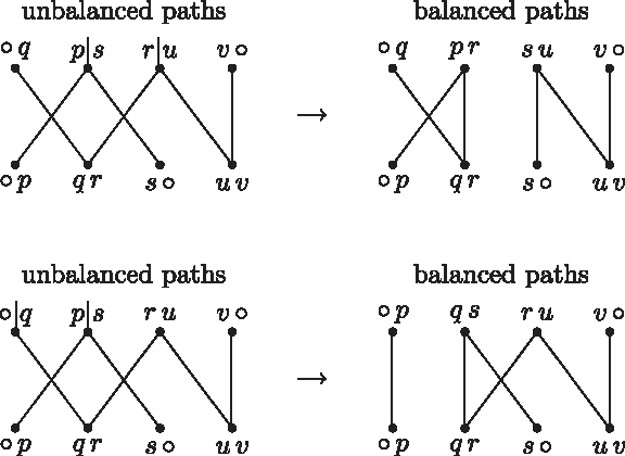
The class of equivalence described in Proposition 12 has three elements and is called an alternative splitting class. An example is shown in Figure 10.

FIG. 10.
Example of equivalence by alternative splitting. Observe that the three pairs of consecutive DCJ operations ρ₁θ₁, ρ₂θ₂ and ρ₃θ₃ transform the adjacencies pv, qr and su into pq, rs and uv.

The last case includes independent and enchained operations whose equivalence classes have six elements:

Class 3

Separation/Recombination: Enchained and independent operations with ps, q○ and r○ as sources and p○, qr and s○ as resultants.

Proposition 13

Given the set of sources S = {ps, q○, r○} and the set of resultants R = {p○, qr, s○}, there are two different pairs of independent operations and four different pairs of enchained operations that transform S into R.

Proof

There are only two independent operations that transform S into R, that are ρ_sep = ({ps} → {p○, s○}) and θ_sep = ({q○, r○} → {qr}). Thus, ρ_sepθ_sep and θ_sepρ_sep are in the class of equivalence of S and R.

Now consider the enchained operations. We know that the first operation will produce only one resultant from R. First we observe that it is not possible to create the resultant qr in the first operation of an enchained pair (if we try to create the resultant qr first, we obtain only the independent pair that was mentioned before). Thus, we can create either the resultant p○ or the resultant s○ in the first operation. Looking to the set of sources we have, we can see that there are two different pairs of sources that could be used in the first operation to create each one of the resultants p○ and s ○. Consequently, there are four possibilities for the first operation of an enchained pair: ρ₁ = ({ps, q○} → {p○, qs}), ρ₂ = ({ps, q○} → {pq, s○}), ρ₃ = ({ps, r○} → {p○, rs}) and ρ₄ = ({ps, r○} → {pr, s○}). For each ρ_i we can obtain a subsequent operation θ_i, such that S(ρ_iθ_i) = S and R(ρ_iθ_i) = R. For each ρ_i there is only one possibility of composing θ_i and we have θ₁ = ({qs, r○} → {qr, s○}), θ₂ = ({pq, r○} → {p○, qr}), θ₃ = ({q○, rs} → {qr, s○}) and θ₄ = ({pr, q○} → {p○, qr}).

Thus, the six pairs ρ_sepθ_sep, θ_sepρ_sep, ρ₁θ₁, ρ₂θ₂, ρ₃θ₃ and ρ₄θ₄ are in the same class of equivalence and there are no more elements in this class. ▪

The class of equivalence described in Proposition 13 has six elements and is called a separation/recombination class. An example is shown in Figure 11.

FIG. 11.
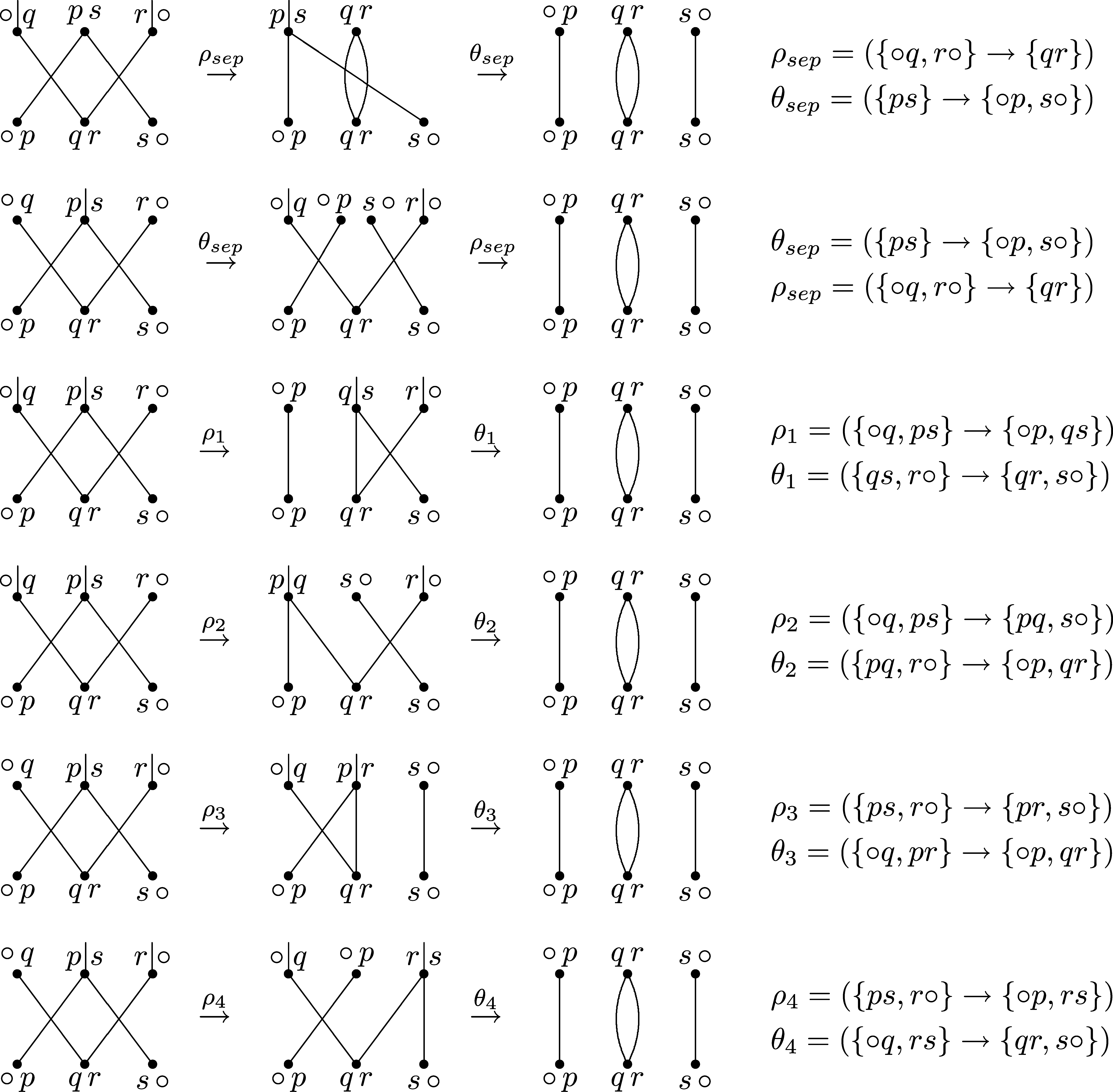
Example of equivalence by separation/recombination. Observe that the six pairs of consecutive DCJ operations ρ_sepθ_sep, θ_sepρ_sep, ρ₁θ₁, ρ₂θ₂, ρ₃θ₃ and ρ₄θ₄ transform the adjacencies q○, ps and r○ into p○, qr and s ○.

Theorem 5

In any optimal DCJ sorting sequence, any pair of consecutive operations can be replaced, leading to one, two, or five other optimal DCJ sorting sequences.

Proof

Let ρ and θ be two consecutive operations in an optimal sorting sequence.

If ρ and θ are independent, and ρθ has four sources or four resultants, then ρθ is in a commutation class with θρ (Proposition 11). If ρ and θ are independent, and ρθ has three sources and three resultants, then ρθ is in a separation/recombination class that contains five other elements (Proposition 13). This includes all independent operations.

If ρ and θ are enchained, we also have two possibilities. When ρ and θ involve at most one telomere, then ρθ is in an alternative splitting class that contains two other elements, and the same is true when ρ and θ involve two telomeres, but have only two sources or only two resultants (Proposition 12).

It remains the case of enchained operations involving two telomeres, with ps, q○, and r○ as sources and p○, qr, and s○ as resultants. In this case, ρθ is also in a separation/recombination class that contains five other elements (Proposition 13).

Each possible pair of consecutive operations belongs to one class of equivalence and can be replaced by one (commutation), two (alternative splitting), or five (separation/recombination) other pairs of consecutive operations. ▪

Observe that, in any class of equivalence given by a set of sources S and a set of resultants R, there is at least one pair of consecutive operations that uses each source in S in the first operation, and at least one pair of consecutive operations that uses each source in S in the second operation. Analogously, there is at least one pair of consecutive operations that creates each resultant in R in the first operation, and at least one pair of consecutive operations that creates each resultant in R in the second operation. Consequently, by replacements we can move any adjacency to a particular position in a sorting sequence.

Theorem 6

Any optimal DCJ sequence can be obtained from any other optimal DCJ sequence by successive replacements of pairs of consecutive operations.

Proof

First note that, if both sequences contain no path recombination, in order to transform one sequence into another, we only have to use commutations and alternative splittings to reconstruct the relative order of the operations sorting each component separately. This is also the case of sequences that contain exactly the same path recombinations (with the same orientation for each recombination).

When the sequences differ in the recombinations, then replacements of the type recombination/separation are also necessary and can be done as follows: if a separation is to be performed, we know that the recombined component has two adjacencies p○ and q○ (all other adjacencies contain only proper extremities); then we first need to use commutations and alternative splittings such that p○ and q○ are in consecutive operations, allowing to perform next a separation; after that we can reconstruct the relative order of the parts using commutations and alternative splittings. If a recombination is to be done, we know that in one part we have an operation ρ = {p○, q○} → {pq} and in the other part we have an operation θ = {rs} → {r○, s○}; we can do a recombination using ρ and θ and then reconstruct the relative order of all operations using commutations and alternative splittings.

Finally, we need only commutations to reconstruct the same global order over all parts (components and recombinations). ▪

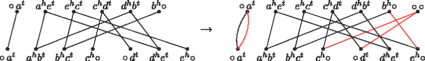
One critical aspect of replacements, including simple commutations, is that they can change the actual nature of the operations over the genomes, as we can see in Figure 12.

FIG. 12.
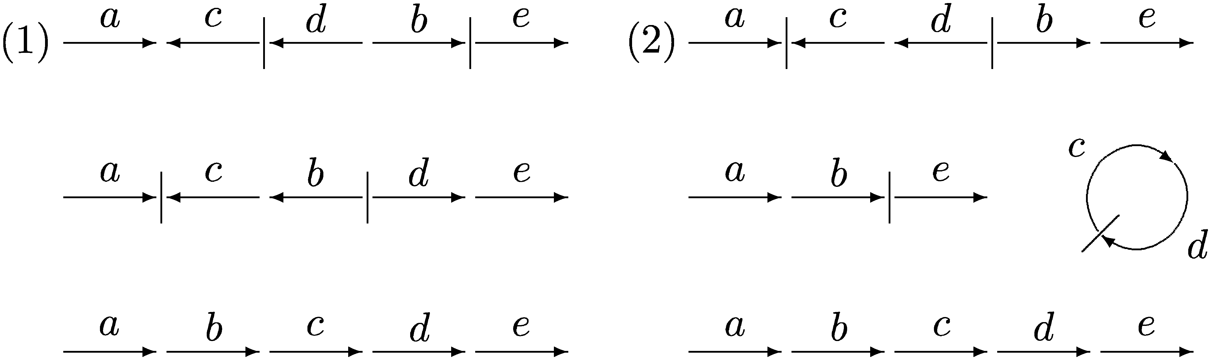
In this graphic representation of the genomes, each arrow represents a marker (from \documentclass{aastex}\usepackage{amsbsy}\usepackage{amsfonts}\usepackage{amssymb}\usepackage{bm}\usepackage{mathrsfs}\usepackage{pifont}\usepackage{stmaryrd}\usepackage{textcomp}\usepackage{portland, xspace}\usepackage{amsmath, amsxtra}\pagestyle{empty}\DeclareMathSizes{10}{9}{7}{6} \begin{document} $${\cal G} = \{ a , b , c , d , e \}$$ \end{document} ) with its corresponding orientation. The commutation of two independent DCJ operations sorting {a^t, a^hc^h, c^td^h, d^tb^t, b^he^t, e^h} into {a^t, a^hb^t, b^hc^t, c^hd^t, d^he^t, e^h} changes the nature of the actual rearrangements. In (1) we have ({c^td^h, b^he^t} → {b^hc^t, d^he^t}) followed by ({a^hc^h, b^td^t} → {a^hb^t, c^hd^t}), a sequence of two inversions, while in (2) we have ({a^hc^h, b^td^t} → {a^hb^t, c^hd^t}) followed by ({c^td^h, b^he^t} → {b^hc^t, d^he^t}), a circular excision followed by a circular integration.

With the results presented here, we demonstrate that all sorting sequences are vertices in the same connected graph and, for each pair of consecutive operations in each sequence, we have one, two or five edges connecting the corresponding vertex to other vertices in the graph. With the methods given in Sections 3 and 4, we are also able to count the number of vertices in this graph, that corresponds to the total number of sorting sequences. However, some important open questions remain. One is the problem of finding the shortest path, that is, the shortest number of replacements between two sorting sequences. Another question, that is actually related to the first, is the problem of avoiding cycles in a walk in the graph. The solutions to these problems could give a measure of similarity between two sorting sequences, leading to a better characterization of the space of solutions.

6. Experiments

6.1. An example illustrating everything

In this section, we want to illustrate the results we presented with one simple example. Let A and B be two genomes, each one composed by one linear and one circular chromosome. The genomes A and B, represented in Figure 13, are defined by their respective sets of adjacencies: \documentclass{aastex}\usepackage{amsbsy}\usepackage{amsfonts}\usepackage{amssymb}\usepackage{bm}\usepackage{mathrsfs}\usepackage{pifont}\usepackage{stmaryrd}\usepackage{textcomp}\usepackage{portland, xspace}\usepackage{amsmath, amsxtra}\pagestyle{empty}\DeclareMathSizes{10}{9}{7}{6}\begin{document} \begin{align} V (A) & = \{ \circ a^h , a^tb^h , b^tc^h , c^td^h , d^t \circ , e^tf^t , e^hf^h \} \\ V (B) & = \{ \circ a^t , a^hb^t , b^hc^t , c^hd^t , d^h \circ , e^tf^h , e^hf^t \} \end{align} \end{document}

The adjacency graph AG(A, B), also represented in Figure 13, has one cycle, one AA-path and one BB-path. We will count the total number of solutions for this example and show subsequent replacements that transform a sequence recombining the AA-path and the BB-path into a sequence sorting all components separately.

FIG. 13.
Genomes A and B, defined by the corresponding sets of adjacencies V(A) = {○ a^h, a^tb^h, b^tc^h, c^td^h, d^t○, e^tf^t, e^hf^h} and V (B) = {○ a^t, a^hb^t, b^hc^t, c^hd^t, d^h○, e^tf^h, e^hf^t}, and their adjacency graph that contains one cycle, one AA-path and one BB-path.

Computing the distance and the total number of sorting sequences. First we can compute the DCJ distance between A and B, with the formula given by Theorem 1, and we have d(A, B) = 6 − 1 − 0 = 5.

We can also compute the number of sequences sorting genome A into B, using the methods described in Sections 3 and 4. The number of sequences that sort A into B without recombining the AA-path and the BB-path is denoted by S_sep: \documentclass{aastex}\usepackage{amsbsy}\usepackage{amsfonts}\usepackage{amssymb}\usepackage{bm}\usepackage{mathrsfs}\usepackage{pifont}\usepackage{stmaryrd}\usepackage{textcomp}\usepackage{portland, xspace}\usepackage{amsmath, amsxtra}\pagestyle{empty}\DeclareMathSizes{10}{9}{7}{6} \begin{document} \begin{align} S_{sep} = \mid EC_4 \otimes UP_4 \otimes UP_4 \mid = {\cal S} (1) \otimes {\cal S} (2) \otimes {\cal S} (2) = [1 , 1] \otimes [3 , 2] \otimes [3 , 2] = [270 , 5]. \end{align} \end{document}

Thus, we have 270 sorting sequences of length 5 without recombinations. The number of sequences that sort A into B recombining the AA-path and the BB-path is denoted by S_rec (the value \documentclass{aastex}\usepackage{amsbsy}\usepackage{amsfonts}\usepackage{amssymb}\usepackage{bm}\usepackage{mathrsfs}\usepackage{pifont}\usepackage{stmaryrd}\usepackage{textcomp}\usepackage{portland, xspace}\usepackage{amsmath, amsxtra}\pagestyle{empty}\DeclareMathSizes{10}{9}{7}{6} \begin{document} $${\cal R} (2 , 2)$$ \end{document} can be obtained in Table 2): \documentclass{aastex}\usepackage{amsbsy}\usepackage{amsfonts}\usepackage{amssymb}\usepackage{bm}\usepackage{mathrsfs}\usepackage{pifont}\usepackage{stmaryrd}\usepackage{textcomp}\usepackage{portland, xspace}\usepackage{amsmath, amsxtra}\pagestyle{empty}\DeclareMathSizes{10}{9}{7}{6} \begin{document} \begin{align} S_{rec} = \mid EC_4 \otimes (UP_4 \oplus UP_4) \mid = {\cal S} (1) \otimes {\cal R} (2 , 2) = [1 , 1] \otimes [208 , 4] = [1040 , 5]. \end{align} \end{document}

This means that we have 1040 sorting sequences of length 5 with recombinations. Consequently, the total number of sequences sorting A into B is 1310.

Transforming a recombining into a non-recombining sorting sequence. Consider the following sequence of operations s_rec = ρ₁ρ₂ρ₃ρ₄ρ₅, sorting A into B: \documentclass{aastex}\usepackage{amsbsy}\usepackage{amsfonts}\usepackage{amssymb}\usepackage{bm}\usepackage{mathrsfs}\usepackage{pifont}\usepackage{stmaryrd}\usepackage{textcomp}\usepackage{portland, xspace}\usepackage{amsmath, amsxtra}\pagestyle{empty}\DeclareMathSizes{10}{9}{7}{6}\begin{document} \begin{align} \rho_1 & = (\{ a^tb^h , b^tc^h \} \to \{ a^tb^t , b^hc^h \}) \\ \rho_2 & = (\{ a^h \circ , a^tb^t \} \to \{ a^t \circ , a^hb^t \}) \\ \rho_3 & = (\{ e^hf^h , e^tf^t \} \to \{ e^hf^t , e^tf^h \}) \\ \rho_4 & = (\{ c^td^h , d^t \circ \} \to \{ c^td^t , d^h \circ \}) \\ \rho_5 & = (\{ b^hc^h , c^td^t \} \to \{ b^hc^t , c^hd^t \}) \end{align} \end{document}

Observe that, since ρ₁ recombines the AA-path and the BB-path, s_rec is a recombining sorting sequence. If we examine the class of equivalence of each pair of consecutive operations in s_rec, we have: ρ₁ρ₂ and ρ₄ρ₅ are in alternative splitting classes (both pairs are composed by enchained operations), while ρ₂ρ₃ and ρ₃ρ₄ are in commutation classes (both pairs are composed by independent operations).

We will show a sequence of five replacements of consecutive operations that transforms s_rec into a non-recombining sorting sequence s_sep:
Replace ρ₁ρ₂ by \documentclass{aastex}\usepackage{amsbsy}\usepackage{amsfonts}\usepackage{amssymb}\usepackage{bm}\usepackage{mathrsfs}\usepackage{pifont}\usepackage{stmaryrd}\usepackage{textcomp}\usepackage{portland, xspace}\usepackage{amsmath, amsxtra}\pagestyle{empty}\DeclareMathSizes{10}{9}{7}{6} \begin{document} $$\rho_1^{\prime} \rho_2^{\prime}$$ \end{document} (alternative splitting):

\documentclass{aastex}\usepackage{amsbsy}\usepackage{amsfonts}\usepackage{amssymb}\usepackage{bm}\usepackage{mathrsfs}\usepackage{pifont}\usepackage{stmaryrd}\usepackage{textcomp}\usepackage{portland, xspace}\usepackage{amsmath, amsxtra}\pagestyle{empty}\DeclareMathSizes{10}{9}{7}{6} \begin{document} $$\rho_1^{\prime} = (\{ a^tb^h , a^h \circ \} \to \{ a^t \circ , a^hb^h \})$$ \end{document}

\documentclass{aastex}\usepackage{amsbsy}\usepackage{amsfonts}\usepackage{amssymb}\usepackage{bm}\usepackage{mathrsfs}\usepackage{pifont}\usepackage{stmaryrd}\usepackage{textcomp}\usepackage{portland, xspace}\usepackage{amsmath, amsxtra}\pagestyle{empty}\DeclareMathSizes{10}{9}{7}{6} \begin{document} $$\rho_2^{\prime} = (\{ a^hb^h , b^tc^h \} \to \{ a^hb^t , b^hc^h \})$$ \end{document}

Replace ρ₄ρ₅ by \documentclass{aastex}\usepackage{amsbsy}\usepackage{amsfonts}\usepackage{amssymb}\usepackage{bm}\usepackage{mathrsfs}\usepackage{pifont}\usepackage{stmaryrd}\usepackage{textcomp}\usepackage{portland, xspace}\usepackage{amsmath, amsxtra}\pagestyle{empty}\DeclareMathSizes{10}{9}{7}{6} \begin{document} $$\rho_4^{\prime} \rho_5^{\prime}$$ \end{document} (alternative splitting):

\documentclass{aastex}\usepackage{amsbsy}\usepackage{amsfonts}\usepackage{amssymb}\usepackage{bm}\usepackage{mathrsfs}\usepackage{pifont}\usepackage{stmaryrd}\usepackage{textcomp}\usepackage{portland, xspace}\usepackage{amsmath, amsxtra}\pagestyle{empty}\DeclareMathSizes{10}{9}{7}{6} \begin{document} $$\rho_4^{\prime} = (\{ b^hc^h , d^t \circ \} \to \{ b^h \circ , c^hd^t \})$$ \end{document}

\documentclass{aastex}\usepackage{amsbsy}\usepackage{amsfonts}\usepackage{amssymb}\usepackage{bm}\usepackage{mathrsfs}\usepackage{pifont}\usepackage{stmaryrd}\usepackage{textcomp}\usepackage{portland, xspace}\usepackage{amsmath, amsxtra}\pagestyle{empty}\DeclareMathSizes{10}{9}{7}{6} \begin{document} $$\rho_5^{\prime} = (\{ b^h \circ , c^td^h \} \to \{ b^hc^t , d^h \circ \})$$ \end{document}

Replace \documentclass{aastex}\usepackage{amsbsy}\usepackage{amsfonts}\usepackage{amssymb}\usepackage{bm}\usepackage{mathrsfs}\usepackage{pifont}\usepackage{stmaryrd}\usepackage{textcomp}\usepackage{portland, xspace}\usepackage{amsmath, amsxtra}\pagestyle{empty}\DeclareMathSizes{10}{9}{7}{6} \begin{document} $$\rho_3 \rho_4^{\prime}$$ \end{document} by \documentclass{aastex}\usepackage{amsbsy}\usepackage{amsfonts}\usepackage{amssymb}\usepackage{bm}\usepackage{mathrsfs}\usepackage{pifont}\usepackage{stmaryrd}\usepackage{textcomp}\usepackage{portland, xspace}\usepackage{amsmath, amsxtra}\pagestyle{empty}\DeclareMathSizes{10}{9}{7}{6} \begin{document} $$\rho_4^{\prime} \rho_3$$ \end{document} (commutation)

Replace \documentclass{aastex}\usepackage{amsbsy}\usepackage{amsfonts}\usepackage{amssymb}\usepackage{bm}\usepackage{mathrsfs}\usepackage{pifont}\usepackage{stmaryrd}\usepackage{textcomp}\usepackage{portland, xspace}\usepackage{amsmath, amsxtra}\pagestyle{empty}\DeclareMathSizes{10}{9}{7}{6} \begin{document} $$\rho_2^{\prime} \rho_4^{\prime}$$ \end{document} by \documentclass{aastex}\usepackage{amsbsy}\usepackage{amsfonts}\usepackage{amssymb}\usepackage{bm}\usepackage{mathrsfs}\usepackage{pifont}\usepackage{stmaryrd}\usepackage{textcomp}\usepackage{portland, xspace}\usepackage{amsmath, amsxtra}\pagestyle{empty}\DeclareMathSizes{10}{9}{7}{6} \begin{document} $$\rho_2^{\prime \prime} \rho_4^{\prime \prime}$$ \end{document} (alternative splitting):

\documentclass{aastex}\usepackage{amsbsy}\usepackage{amsfonts}\usepackage{amssymb}\usepackage{bm}\usepackage{mathrsfs}\usepackage{pifont}\usepackage{stmaryrd}\usepackage{textcomp}\usepackage{portland, xspace}\usepackage{amsmath, amsxtra}\pagestyle{empty}\DeclareMathSizes{10}{9}{7}{6} \begin{document} $$\rho_2^{\prime \prime} = (\{ a^hb^h , d^t \circ \} \to \{ b^h \circ , a^hd^t \})$$ \end{document}

\documentclass{aastex}\usepackage{amsbsy}\usepackage{amsfonts}\usepackage{amssymb}\usepackage{bm}\usepackage{mathrsfs}\usepackage{pifont}\usepackage{stmaryrd}\usepackage{textcomp}\usepackage{portland, xspace}\usepackage{amsmath, amsxtra}\pagestyle{empty}\DeclareMathSizes{10}{9}{7}{6} \begin{document} $$\rho_4^{\prime \prime} = (\{ a^hd^t , b^tc^h \} \to \{a^hb^t , c^hd^t \})$$ \end{document}

Replace \documentclass{aastex}\usepackage{amsbsy}\usepackage{amsfonts}\usepackage{amssymb}\usepackage{bm}\usepackage{mathrsfs}\usepackage{pifont}\usepackage{stmaryrd}\usepackage{textcomp}\usepackage{portland, xspace}\usepackage{amsmath, amsxtra}\pagestyle{empty}\DeclareMathSizes{10}{9}{7}{6} \begin{document} $$\rho_1^{\prime} \rho_2^{\prime \prime}$$ \end{document} by \documentclass{aastex}\usepackage{amsbsy}\usepackage{amsfonts}\usepackage{amssymb}\usepackage{bm}\usepackage{mathrsfs}\usepackage{pifont}\usepackage{stmaryrd}\usepackage{textcomp}\usepackage{portland, xspace}\usepackage{amsmath, amsxtra}\pagestyle{empty}\DeclareMathSizes{10}{9}{7}{6} \begin{document} $$\rho_1^{\prime \prime} \rho_2^{\prime \prime \prime}$$ \end{document} (recombination/separation):

\documentclass{aastex}\usepackage{amsbsy}\usepackage{amsfonts}\usepackage{amssymb}\usepackage{bm}\usepackage{mathrsfs}\usepackage{pifont}\usepackage{stmaryrd}\usepackage{textcomp}\usepackage{portland, xspace}\usepackage{amsmath, amsxtra}\pagestyle{empty}\DeclareMathSizes{10}{9}{7}{6} \begin{document} $$\rho_1^{\prime \prime} = (\{ a^h \circ , d^t \circ \} \to \{ a^hd^t \})$$ \end{document}

\documentclass{aastex}\usepackage{amsbsy}\usepackage{amsfonts}\usepackage{amssymb}\usepackage{bm}\usepackage{mathrsfs}\usepackage{pifont}\usepackage{stmaryrd}\usepackage{textcomp}\usepackage{portland, xspace}\usepackage{amsmath, amsxtra}\pagestyle{empty}\DeclareMathSizes{10}{9}{7}{6} \begin{document} $$\rho_2^{\prime \prime \prime} = (\{ a^tb^h \} \to \{ a^t \circ , b^h \circ \})$$ \end{document}

After the replacements above, we have the sequence of operations \documentclass{aastex}\usepackage{amsbsy}\usepackage{amsfonts}\usepackage{amssymb}\usepackage{bm}\usepackage{mathrsfs}\usepackage{pifont}\usepackage{stmaryrd}\usepackage{textcomp}\usepackage{portland, xspace}\usepackage{amsmath, amsxtra}\pagestyle{empty}\DeclareMathSizes{10}{9}{7}{6} \begin{document} $$s_{sep} = \rho_1^{\prime \prime} \rho_2^{\prime \prime \prime} \rho_4^{\prime \prime} \rho_3 \rho_5^{\prime}$$ \end{document} , that also sorts A into B. Since the operation \documentclass{aastex}\usepackage{amsbsy}\usepackage{amsfonts}\usepackage{amssymb}\usepackage{bm}\usepackage{mathrsfs}\usepackage{pifont}\usepackage{stmaryrd}\usepackage{textcomp}\usepackage{portland, xspace}\usepackage{amsmath, amsxtra}\pagestyle{empty}\DeclareMathSizes{10}{9}{7}{6} \begin{document} $$p_1^{\prime \prime}$$ \end{document} separates the AA-path and the operation \documentclass{aastex}\usepackage{amsbsy}\usepackage{amsfonts}\usepackage{amssymb}\usepackage{bm}\usepackage{mathrsfs}\usepackage{pifont}\usepackage{stmaryrd}\usepackage{textcomp}\usepackage{portland, xspace}\usepackage{amsmath, amsxtra}\pagestyle{empty}\DeclareMathSizes{10}{9}{7}{6} \begin{document} $$p_2^{\prime \prime \prime}$$ \end{document} separates the BB-path, s_sep is not a recombining sequence. If we now examine the class of equivalence of each pair of consecutive operations in s_sep, we can see that \documentclass{aastex}\usepackage{amsbsy}\usepackage{amsfonts}\usepackage{amssymb}\usepackage{bm}\usepackage{mathrsfs}\usepackage{pifont}\usepackage{stmaryrd}\usepackage{textcomp}\usepackage{portland, xspace}\usepackage{amsmath, amsxtra}\pagestyle{empty}\DeclareMathSizes{10}{9}{7}{6} \begin{document} $$\rho_1^{\prime \prime} \rho_2^{\prime \prime \prime}$$ \end{document} is in a separation/recombination class, while \documentclass{aastex}\usepackage{amsbsy}\usepackage{amsfonts}\usepackage{amssymb}\usepackage{bm}\usepackage{mathrsfs}\usepackage{pifont}\usepackage{stmaryrd}\usepackage{textcomp}\usepackage{portland, xspace}\usepackage{amsmath, amsxtra}\pagestyle{empty}\DeclareMathSizes{10}{9}{7}{6} \begin{document} $$\rho_2^{\prime \prime \prime} \rho_4^{\prime \prime}, \ \rho_4^{\prime \prime} \rho_3 \ {\rm and} \ \rho_3 \rho_5^{\prime}$$ \end{document} are in commutation classes (all pairs are composed by independent operations).

6.2. Comparing human, chimpanzee, and rhesus monkey

From Alekseyev and Pevzner (2009), we obtained a database with the synteny blocks of the genomes of human (Homo sapiens), chimpanzee (Pan troglodytes), and rhesus monkey (Macaca mulatta), and used the methods described in Sections 3 and 4 to compute the number of DCJ sequences for the pairwise comparison of these genomes. The results are shown in Table 4.

Table 4.
Counting DCJ Sorting Sequences between Human, Chimpanzee, and Rhesus Monkey Genomes (Data Obtained from Alekseyev and Pevzner, 2009)

Genomes No. big EC No. big BP No. UP DCJ dist. Sequences without rec. All DCJ sequences

Human versus chimpanzee 18 1 1 + 0 22 ≃2.53 × 10²¹ ≃2.53 × 10²¹

Human versus monkey 59 7 2 + 4 106 ≃1.23 × 10¹⁷⁷ ≃2.19 × 10¹⁷⁹

Chimpanzee versus monkey 68 8 1 + 4 114 ≃1.53 × 10¹⁹³ ≃2.15 × 10¹⁹⁴

For each pairwise comparison, the number of sorting sequences is very large and is thus presented approximately (although it can be computed exactly). Observe that the number of paths is usually much smaller than the number of cycles in all pairwise comparisons. Looking at the human versus chimpanzee comparison in particular, we notice that it results in only one unbalanced path, thus none of its sorting sequences can be obtained by recombining unbalanced into balanced paths. This means that the formula of Theorem 4 corresponds to the exact number of sequences in this case.

We observed that the number of paths and, more particularly, the number of unbalanced paths in the corresponding adjacency graphs is small. Consequently, the enumeration of simultaneous recombinations for these three comparisons do not require space and time consuming computation to be obtained. Comparing the human and chimpanzee genomes, for instance, we have only one unbalanced path, so it is not possible to recombine unbalanced into balanced paths. Since big paths occur when some extremities of linear chromosomes are different in the two analyzed genomes, our results suggest that this is unlikely to happen when the genomes are closely related.

7. Conclusion

In this work, we studied the solution space of the sorting by DCJ problem. We proposed a formula that gives a lower bound to the number of all optimal DCJ sequences sorting one genome into another. This formula can be easily and quickly computed and corresponds to the exact number of sorting sequences for a particular subset of instances of the problem. We could also identify the structures of the compared genomes that cause the increase of the number of solutions with respect to the given lower bound, designing an algorithm to compute the number of DCJ sorting sequences to any instance of the problem. We used this algorithm to compute the number of sequences for three pairwise comparisons: human versus chimpanzee, human versus rhesus monkey, and chimpanzee versus rhesus monkey.

Furthermore, we were able to demonstrate that all sorting sequences are connected, that is, any optimal sequence can be transformed into any other one by replacements (due to commutation, alternative splitting or separation/recombination) of pairs of consecutive operations. However, the problem of finding the shortest number of replacements between two sorting sequences is still open. The solution to this question could give a measure of similarity between two sorting sequences, leading to a better characterization of the space of solutions.

Unbalanced paths	Balanced paths	Even cycles	Sequence length	Number of sequences
UP ₂	BP ₃	EC ₄	1	1
UP ₄	BP ₅	EC ₆	2	3
UP ₆	BP ₇	EC ₈	3	16
UP ₈	BP ₉	EC ₁₀	4	125
UP ₁₀	BP ₁₁	EC ₁₂	5	1296
UP ₁₂	BP ₁₃	EC ₁₄	6	16807
\documentclass{aastex}\usepackage{amsbsy}\usepackage{amsfonts}\usepackage{amssymb}\usepackage{bm}\usepackage{mathrsfs}\usepackage{pifont}\usepackage{stmaryrd}\usepackage{textcomp}\usepackage{portland, xspace}\usepackage{amsmath, amsxtra}\pagestyle{empty}\DeclareMathSizes{10}{9}{7}{6} \begin{document} $$\vdots$$ \end{document}	\documentclass{aastex}\usepackage{amsbsy}\usepackage{amsfonts}\usepackage{amssymb}\usepackage{bm}\usepackage{mathrsfs}\usepackage{pifont}\usepackage{stmaryrd}\usepackage{textcomp}\usepackage{portland, xspace}\usepackage{amsmath, amsxtra}\pagestyle{empty}\DeclareMathSizes{10}{9}{7}{6} \begin{document} $$\vdots$$ \end{document}	\documentclass{aastex}\usepackage{amsbsy}\usepackage{amsfonts}\usepackage{amssymb}\usepackage{bm}\usepackage{mathrsfs}\usepackage{pifont}\usepackage{stmaryrd}\usepackage{textcomp}\usepackage{portland, xspace}\usepackage{amsmath, amsxtra}\pagestyle{empty}\DeclareMathSizes{10}{9}{7}{6} \begin{document} $$\vdots$$ \end{document}	\documentclass{aastex}\usepackage{amsbsy}\usepackage{amsfonts}\usepackage{amssymb}\usepackage{bm}\usepackage{mathrsfs}\usepackage{pifont}\usepackage{stmaryrd}\usepackage{textcomp}\usepackage{portland, xspace}\usepackage{amsmath, amsxtra}\pagestyle{empty}\DeclareMathSizes{10}{9}{7}{6} \begin{document} $$\vdots$$ \end{document}	\documentclass{aastex}\usepackage{amsbsy}\usepackage{amsfonts}\usepackage{amssymb}\usepackage{bm}\usepackage{mathrsfs}\usepackage{pifont}\usepackage{stmaryrd}\usepackage{textcomp}\usepackage{portland, xspace}\usepackage{amsmath, amsxtra}\pagestyle{empty}\DeclareMathSizes{10}{9}{7}{6} \begin{document} $$\vdots$$ \end{document}
UP _2ℓ	BP _2ℓ+1	EC _2ℓ+2	ℓ	(ℓ + 1)^ℓ−1

AA-path d = ℓ_A	BB-path d = ℓ_B	Non-recombining: \documentclass{aastex}\usepackage{amsbsy}\usepackage{amsfonts}\usepackage{amssymb}\usepackage{bm}\usepackage{mathrsfs}\usepackage{pifont}\usepackage{stmaryrd}\usepackage{textcomp}\usepackage{portland, xspace}\usepackage{amsmath, amsxtra}\pagestyle{empty}\DeclareMathSizes{10}{9}{7}{6} \begin{document} $${\cal W} (\ell_A , \ell_B)$$ \end{document}	All recombining solutions: \documentclass{aastex}\usepackage{amsbsy}\usepackage{amsfonts}\usepackage{amssymb}\usepackage{bm}\usepackage{mathrsfs}\usepackage{pifont}\usepackage{stmaryrd}\usepackage{textcomp}\usepackage{portland, xspace}\usepackage{amsmath, amsxtra}\pagestyle{empty}\DeclareMathSizes{10}{9}{7}{6} \begin{document} $${\cal R} (\ell_A , \ell_B) = 2 ({\cal S} (\ell_A + \ell_B) - {\cal W} (\ell_A , \ell_B))$$ \end{document}
1	1	1	4
1	2	4	24
1	3	27	196
1	4	256	2, 080
1	5	3, 125	27, 364
1	6	46, 656	430, 976
1	7	823, 543	7, 918, 852
1	8	16, 777, 216	166, 445, 568
1	9	387, 420, 489	3, 941, 054, 404
2	1	4	24
2	2	21	208
2	3	176	2, 240
2	4	1, 995	29, 624
2	5	28, 344	467, 600
2	6	482, 825	8, 600, 288
2	7	9, 576, 160	180, 847, 680
2	8	216, 559, 287	4, 282, 776, 808
3	1	27	196
3	2	176	2, 240
3	3	1, 765	30, 084
3	4	23, 304	477, 680
3	5	378, 007	8, 809, 924
3	6	7, 238, 944	185, 522, 112
3	7	159, 444, 585	4, 397, 006, 212

Algorithm 1. Computing all matchings in a complete bipartite graph
Input: The partitions P₁ and P₂ with all AA-paths and all BB-paths, respectively
Output: The set M with all possible matchings of sizes \documentclass{aastex}\usepackage{amsbsy}\usepackage{amsfonts}\usepackage{amssymb}\usepackage{bm}\usepackage{mathrsfs}\usepackage{pifont}\usepackage{stmaryrd}\usepackage{textcomp}\usepackage{portland, xspace}\usepackage{amsmath, amsxtra}\pagestyle{empty}\DeclareMathSizes{10}{9}{7}{6} \begin{document} $$1 , 2 , \ldots , \min (\mid P_1 \mid , \mid P_2 \mid)$$ \end{document}
\documentclass{aastex}\usepackage{amsbsy}\usepackage{amsfonts}\usepackage{amssymb}\usepackage{bm}\usepackage{mathrsfs}\usepackage{pifont}\usepackage{stmaryrd}\usepackage{textcomp}\usepackage{portland, xspace}\usepackage{amsmath, amsxtra}\pagestyle{empty}\DeclareMathSizes{10}{9}{7}{6} \begin{document} $$P_{12} \leftarrow \{ \{e_1 , e_2 \} \ \mid \ e_1 \in P_1 \ {\rm and} \ e_2 \in P_2 \}$$ \end{document} [P₁₂ contains \|P₁\| × \|P₂\| pairs]
M₁ ← P₁₂ [the set of all matchings of size 1]
M ← M₁ [the set of all matchings]
for each \documentclass{aastex}\usepackage{amsbsy}\usepackage{amsfonts}\usepackage{amssymb}\usepackage{bm}\usepackage{mathrsfs}\usepackage{pifont}\usepackage{stmaryrd}\usepackage{textcomp}\usepackage{portland, xspace}\usepackage{amsmath, amsxtra}\pagestyle{empty}\DeclareMathSizes{10}{9}{7}{6} \begin{document} $$k = 2 , 3 , \ldots , \min (\mid P_1 \mid , \mid P_2 \mid)$$ \end{document} do
M_k ← all extensions of each matching m in M_k_− 1 with a new pair p in P₁₂ such that the elements in p do not appear in any other pair of m [the set of all matchings of size k]
\documentclass{aastex}\usepackage{amsbsy}\usepackage{amsfonts}\usepackage{amssymb}\usepackage{bm}\usepackage{mathrsfs}\usepackage{pifont}\usepackage{stmaryrd}\usepackage{textcomp}\usepackage{portland, xspace}\usepackage{amsmath, amsxtra}\pagestyle{empty}\DeclareMathSizes{10}{9}{7}{6} \begin{document} $$M \leftarrow M \cup M_k$$ \end{document} [integrate M_k to the set of all matchings]
end for
return M [M is the final set with all matchings]

mⁿ	1	2	3	4	5	6	7	8	9	10
1	1	2	3	4	5	6	7	8	9	10
2	2	6	12	20	30	42	56	72	90	110
3	3	12	33	72	135	228	357	528	747	1020
4	4	20	72	208	500	1044	1960	3392	5508	8500
5	5	30	135	500	1545	4050	9275	19080	36045	63590
6	6	42	228	1044	4050	13326	37632	93288	207774	424050
7	7	56	357	1960	9275	37632	130921	394352	1047375	2501800
8	8	72	528	3392	19080	93288	394352	1441728	4596552	12975560
9	9	90	747	5508	36045	207774	1047375	4596552	17572113	58941090
10	10	110	1020	8500	63590	424050	2501800	12975560	58941090	234662230

Genomes	No. big EC	No. big BP	No. UP	DCJ dist.	Sequences without rec.	All DCJ sequences
Human versus chimpanzee	18	1	1 + 0	22	≃2.53 × 10²¹	≃2.53 × 10²¹
Human versus monkey	59	7	2 + 4	106	≃1.23 × 10¹⁷⁷	≃2.19 × 10¹⁷⁹
Chimpanzee versus monkey	68	8	1 + 4	114	≃1.53 × 10¹⁹³	≃2.15 × 10¹⁹⁴

Footnotes

Acknowledgments

We are grateful to Aïda Ouangraoua and Anne Bergeron for helpful discussions about the recombination of a pair of unbalanced paths and useful comments on an earlier version of the manuscript.

Disclosure Statement

No competing financial interests exist.

References

Alekseyev

M.A.

, Pevzner

P.A.

2009. Breakpoint graphs and ancestral genome reconstructions. Genome Res., 19:943–957.

Bergeron

, Chauve

, Hartmann

et al. 2002. On the properties of sequences of reversals that sort a signed permutation. Proc. JOBIM, 2002:99–108.

Bergeron

, Mixtacki

, Stoye

2006. A unifying view of genome rearrangements. Lect. Notes Comput. Sci., 4175:163–173.

Braga

M.D.V.

, Sagot

M.-F.

, Scornavacca

et al. 2008. Exploring the solution space of sorting by reversals with experiments and an application to evolution. IEEE/ACM Trans. Comput. Biol. Bioinform., 5:348–356.

Braga

M.D.V.

, Stoye

2009. Counting all DCJ sorting scenarios. Lect. Notes Bioinform., 5817:36–47.

Fertin

, Labarre

, Rusu

et al. 2009. Combinatorics of Genome Rearrangements. The MIT Press: Cambridge, MA.

Hannenhalli

, Pevzner

1995. Transforming men into mice (polynomial algorithm for genomic distance problem) Proc. FOCS, 1995:581–592.

Ouangraoua

, Bergeron

2010. Parking functions, labeled trees and DCJ sorting scenarios. Lect. Notes Bioinform., 5817:24–35.

Sankoff

1992. Edit distance for genome comparison based on non-local operations. Lect. Notes Comput. Sci., 644:121–135.

10.

Siepel

2003. An algorithm to enumerate sorting reversals for signed permutations. J. Comput. Biol., 10:575–597.

11.

Tannier

, Zheng

, Sankoff

2009. Multichromosomal median and halving problems under different genomic distances. BMC Bioinform., 10:120.

12.

Yancopoulos

, Attie

, Friedberg

2005. Efficient sorting of genomic permutations by translocation, inversion and block interchange. Bioinformatics, 21:3340–3346.

13.

Zeilberger

2010. Yet another proof of Cayley's formula for the number of labelled trees. www.math.rutgers.edu/∼zeilberg/mamarim/mamarimPDF/cayley.pdf. July 1 2010.

\documentclass{aastex}\usepackage{amsbsy}\usepackage{amsfonts}\usepackage{amssymb}\usepackage{bm}\usepackage{mathrsfs}\usepackage{pifont}\usepackage{stmaryrd}\usepackage{textcomp}\usepackage{portland, xspace}\usepackage{amsmath, amsxtra}\pagestyle{empty}\DeclareMathSizes{10}{9}{7}{6} \begin{document} $$X = \sum\nolimits_{i = 1}^{\ell_A - 1} (i + 1) \times {\cal W} (i , \ell_B) \otimes {\cal S} (\ell_A - i - 1)$$ \end{document}	(reduce the AA-path extracting a (2[ℓ_A − i − 1] + 2)-cycle)
\documentclass{aastex}\usepackage{amsbsy}\usepackage{amsfonts}\usepackage{amssymb}\usepackage{bm}\usepackage{mathrsfs}\usepackage{pifont}\usepackage{stmaryrd}\usepackage{textcomp}\usepackage{portland, xspace}\usepackage{amsmath, amsxtra}\pagestyle{empty}\DeclareMathSizes{10}{9}{7}{6} \begin{document} $$Y = \sum\nolimits_{i = 1}^{\ell_B - 1} i \times {\cal W} (\ell_A , i) \otimes {\cal S} (\ell_B - i - 1)$$ \end{document}	(reduce the BB-path extracting a (2[ℓ_B − i − 1] + 2)-cycle)
\documentclass{aastex}\usepackage{amsbsy}\usepackage{amsfonts}\usepackage{amssymb}\usepackage{bm}\usepackage{mathrsfs}\usepackage{pifont}\usepackage{stmaryrd}\usepackage{textcomp}\usepackage{portland, xspace}\usepackage{amsmath, amsxtra}\pagestyle{empty}\DeclareMathSizes{10}{9}{7}{6} \begin{document} $$Z = {\cal S} (\ell_A - 1) \otimes {\cal S} (\ell_B)$$ \end{document}	(separate the paths)