Gene Expression Complex Networks: Synthesis,Identification,and Analysis

Abstract

Thanks to recent advances in molecular biology, allied to an ever increasing amount of experimental data, the functional state of thousands of genes can now be extracted simultaneously by using methods such as cDNA microarrays and RNA-Seq. Particularly important related investigations are the modeling and identification of gene regulatory networks from expression data sets. Such a knowledge is fundamental for many applications, such as disease treatment, therapeutic intervention strategies and drugs design, as well as for planning high-throughput new experiments. Methods have been developed for gene networks modeling and identification from expression profiles. However, an important open problem regards how to validate such approaches and its results. This work presents an objective approach for validation of gene network modeling and identification which comprises the following three main aspects: (1) Artificial Gene Networks (AGNs) model generation through theoretical models of complex networks, which is used to simulate temporal expression data; (2) a computational method for gene network identification from the simulated data, which is founded on a feature selection approach where a target gene is fixed and the expression profile is observed for all other genes in order to identify a relevant subset of predictors; and (3) validation of the identified AGN-based network through comparison with the original network. The proposed framework allows several types of AGNs to be generated and used in order to simulate temporal expression data. The results of the network identification method can then be compared to the original network in order to estimate its properties and accuracy. Some of the most important theoretical models of complex networks have been assessed: the uniformly-random Erdös-Rényi (ER), the small-world Watts-Strogatz (WS), the scale-free Barabási-Albert (BA), and geographical networks (GG). The experimental results indicate that the inference method was sensitive to average degree 〈k〉 variation, decreasing its network recovery rate with the increase of 〈k〉. The signal size was important for the inference method to get better accuracy in the network identification rate, presenting very good results with small expression profiles. However, the adopted inference method was not sensible to recognize distinct structures of interaction among genes, presenting a similar behavior when applied to different network topologies. In summary, the proposed framework, though simple, was adequate for the validation of the inferred networks by identifying some properties of the evaluated method, which can be extended to other inference methods.

1. Introduction

Genetic regulation can be viewed as a complex system with many forward and feedback signals. However, how the control mechanisms such as transcript and proteins levels are interconnected and regulated remains very poorly understood. Much effort has been spent to investigate these control mechanisms and their functional relations. One way to better understand these functional relations is to take into account the temporal evolution of gene expression. In particular, the development of massive data collection techniques, such as cDNA microarrays and RNA-Seq (Wang et al., 2009), has paved the way to simultaneous monitoring the several components of the cellular estate along multiples instants of time. These high-throughput techniques, complemented by computational methods, make possible the reconstruction of large-scale networks, which can provide important insights about the topological organization of these networks and can explain relationships between topological and biological properties of the network. This information is particularly relevant while analysing the behavior of genes activity (transcriptions levels), its functional relations, and for estimation of gene regulatory networks (GRNs) (Shmulevich and Dougherty, 2007).

The reconstruction of GRNs from expression profiles is founded on the hypothesis that the information about the functional state of an organism is determined by its genes expression patterns, which constitutes the central dogma of molecular biology (D'Haeseleer et al., 1999; Nelson and Cox, 2004). The GRN approach yields useful models to understand the regulatory pathways, to measure changes that occur during cellular cycle, and to identify environmental effects. Such an information provides insights about how the genes are regulated, improving the knowledge about the functioning of living organisms at the molecular level. Therefore, the identification of GRNs from gene expression patterns represents a particular important challenge in bioinformatics research, e.g., motivating the DREAM project (DREAM, 2009).

In general, it is not possible to assure the quality of inferred networks due to the lack of information about the biological organism. In this context, it is very important to use computational simulations to do it. By adopting simulations, the gold standard is known, which makes possible to investigate prior information, such as network topology classes (e.g., random or scale-free networks), or the system dynamics in spite of some hypothesis.

In order to identify some of the fundamental mathematical principles that underlie large nets of interacting genes, Kauffman (1969, 1993) proposed the use of binary “genes” and Boolean functions. The dynamics of this network model is defined by selecting, for each target vertex, a set of arbitrary chosen predictor vertices together with combinatorial logic circuits. The value assumed by the target is determined by applying the corresponding logic circuit to its predictors values. This model is known as Boolean Networks (BNs). After this pioneering work, several other methods were proposed for modeling and identification of gene regulatory networks. Some reviews are available (D'haeseleer et al., 2000; de Jong, 2002; Styczynski and Stephanopoulos, 2005; Schllit and Brazma, 2007; Karlebach and Shamir, 2008; Hecker et al., 2009).

Validation of the identified networks requires prior knowledge about the real gene connections and its functional relations, which are often unknown or incomplete. In this way, an important open problem remains: how to validate the results of network identification methods? One approach to objectively tackle this issue is to take into account computational gene network models (Mendes et al., 2003; Lopes et al., 2008a) for which the mechanisms are completely known.

Even though the Boolean formalism is seemingly simple, this model has been used to qualitatively describe the overall behavior of gene networks. This property allows the analysis of data sets in a global way, which presents some characteristics of real GRNs (Kauffman et al., 2003; Serra et al., 2004; Shmulevich et al., 2005). Recently BNs were successfully applied for modeling and/or simulating biological networks and processes (Sánchez and Thieffry, 2001; Albert and Othmer, 2003; Li et al., 2004; Espinosa-Soto et al., 2004; Li and Lu, 2005; Faure et al., 2006; Quayle and Bullock, 2006; Li et al., 2006; Klamt et al., 2007; Davidich and Bornholdt, 2008; Albert et al., 2008; Hickman and Hodgman, 2009). On the other hand, models based on differential equations (Mendes et al., 2003; de Jong et al., 2003; Van den Bulcke et al., 2006; Haynes and Brent, 2009) allows the generation of a detailed network dynamics. However, the determination of the parameters to recover the network would require high-quality data (Karlebach and Shamir, 2008) and a larger amount (Wahde and Hertz, 2000) than is generally available. Therefore, the BNs are a suitable model to generalize and capture the behavior of biological systems at the highest level (qualitative), in face of the limited number of temporal samples, the high system dimension and the noisy nature of the expression measurements.

Although BNs have been useful in several cases, one important limitation is their inherent determinism, which makes the assumption of an environment with no uncertainty. On the other hand, it is important to consider that a cell is an open system and can receive external stimuli. Depending on external conditions at a given instant of time, the cell can change its dynamics (Shmulevich and Dougherty, 2007). In this context, we have developed a new approach to generate Artificial Gene Networks (AGNs) in order to investigate the properties of GRNs inference methods under certain conditions.

The AGN model proposed in this work was built by adopting the probabilistic Boolean network (PBN) (Shmulevich et al., 2002a,b) approach, that preserve the well known properties of BNs and avoid its deterministic rigidity. This model allows the study and identification of high-level properties of gene networks and their interactions, without the necessity low-level biochemical descriptions as adopted by other works (de la Fuente et al., 2004; Bansal et al., 2007; Soranzo et al., 2007) that analyse the inference methods.

The AGN model proposed here is based on theoretical models of complex networks (Albert and Barabási, 2002; Newman, 2003; da F. Costa et al., 2007), which define its topology. The dynamics of the AGN is then obtained by applying transition functions, which simulate the expression dynamics according to the imposed regulations. Both deterministic and stochastic networks may be generated and simulated, depending on the chosen transition functions (whether deterministic or stochastic). A specific network identification method (Barrera et al., 2007) was chosen to illustrate our approach, and the identified networks were validated with respect to four particularly relevant AGN models.

The identification method used in this work is based on a feature selection approach where a target gene is fixed and the temporal expression profile is observed for all genes, followed by the estimation of the mean conditional entropy as a criterion function in order to choose a subset of predictors genes (entropy minimization). Respectively implied directional edges are then created connecting from predictors to target genes. This procedure is repeated for each target gene. The network identification method was chosen after a comparative analysis (Lopes et al., 2009), in which it presented enhanced results. Figure 1 gives an overview of the proposed framework.

FIG. 1.

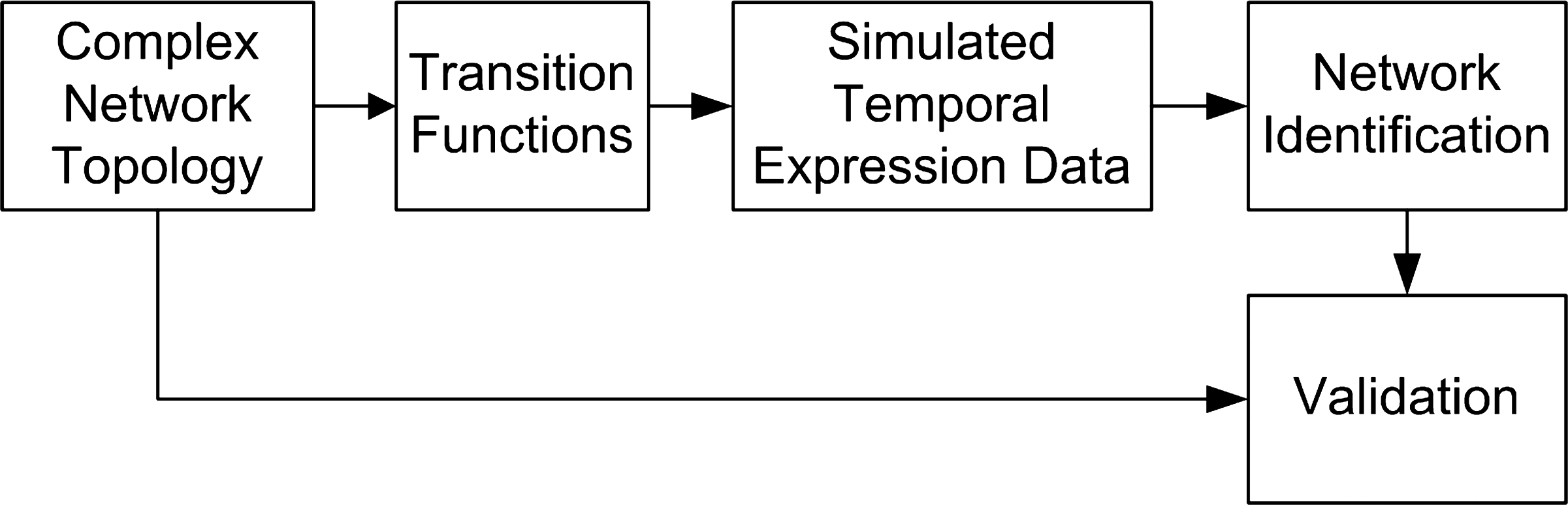
Overview of the proposed framework, showing its stages and how they are connected.

2. Methods

2.1. Conceptual AGN model

In the context of this work, an artificial gene network (AGN) is a directed graph in which the vertices represent genes, while the edges stand for the dependencies between respectively linked genes, i.e., direct influence. These influences can be expressed in a deterministic or stochastic way. The edges in an AGN allow us to express directly the dependence relationships, so that the resulting topology makes these relationships explicit. For this reason, graphs have become the most common metaphor for representing conceptual dependencies (Pearl, 1988).

More formally, an AGN is a tuple G = (V, E, S, Ψ), in which \documentclass{aastex}\usepackage{amsbsy}\usepackage{amsfonts}\usepackage{amssymb}\usepackage{bm}\usepackage{mathrsfs}\usepackage{pifont}\usepackage{stmaryrd}\usepackage{textcomp}\usepackage{portland,xspace}\usepackage{amsmath,amsxtra}\pagestyle{empty}\DeclareMathSizes{10}{9}{7}{6} \begin{document} $$V = \{ v_1 , v_2 , \ldots , v_n \} $$\end{document} represents a set of n vertices or “genes,” connected by a set \documentclass{aastex}\usepackage{amsbsy}\usepackage{amsfonts}\usepackage{amssymb}\usepackage{bm}\usepackage{mathrsfs}\usepackage{pifont}\usepackage{stmaryrd}\usepackage{textcomp}\usepackage{portland,xspace}\usepackage{amsmath,amsxtra}\pagestyle{empty}\DeclareMathSizes{10}{9}{7}{6} \begin{document} $$E = \{ e_1 , e_2 , \ldots , e_m \} $$\end{document} of m edges, where each edge e_l = (v_i, v_j) is an ordered pair of vertices in G, from v_i to v_j. Each vertex (gene) can assume a numerical value from a set \documentclass{aastex}\usepackage{amsbsy}\usepackage{amsfonts}\usepackage{amssymb}\usepackage{bm}\usepackage{mathrsfs}\usepackage{pifont}\usepackage{stmaryrd}\usepackage{textcomp}\usepackage{portland,xspace}\usepackage{amsmath,amsxtra}\pagestyle{empty}\DeclareMathSizes{10}{9}{7}{6} \begin{document} $$D \subset {\mathbb Z}$$\end{document} , i.e., \documentclass{aastex}\usepackage{amsbsy}\usepackage{amsfonts}\usepackage{amssymb}\usepackage{bm}\usepackage{mathrsfs}\usepackage{pifont}\usepackage{stmaryrd}\usepackage{textcomp}\usepackage{portland,xspace}\usepackage{amsmath,amsxtra}\pagestyle{empty}\DeclareMathSizes{10}{9}{7}{6} \begin{document} $$v_i \in D , i = 1 , 2 , \ldots , n$$\end{document} . The vertices and edges define the network topology, while the input edges of a vertex represent the genes that have direct influence on its behavior.

The set of states of an AGN is defined as \documentclass{aastex}\usepackage{amsbsy}\usepackage{amsfonts}\usepackage{amssymb}\usepackage{bm}\usepackage{mathrsfs}\usepackage{pifont}\usepackage{stmaryrd}\usepackage{textcomp}\usepackage{portland,xspace}\usepackage{amsmath,amsxtra}\pagestyle{empty}\DeclareMathSizes{10}{9}{7}{6} \begin{document} $$S = \{ \vec{s}_1 , \vec{s}_2 , \ldots , \vec{s}_z \} $$\end{document} , where the number of possible states of an AGN is defined by z = Dⁿ. Each v_i represents the state (expression value) of gene i, and the network state \documentclass{aastex}\usepackage{amsbsy}\usepackage{amsfonts}\usepackage{amssymb}\usepackage{bm}\usepackage{mathrsfs}\usepackage{pifont}\usepackage{stmaryrd}\usepackage{textcomp}\usepackage{portland,xspace}\usepackage{amsmath,amsxtra}\pagestyle{empty}\DeclareMathSizes{10}{9}{7}{6} \begin{document} $$\vec{s}_j$$\end{document} is determined by the configuration of all gene values. The set \documentclass{aastex}\usepackage{amsbsy}\usepackage{amsfonts}\usepackage{amssymb}\usepackage{bm}\usepackage{mathrsfs}\usepackage{pifont}\usepackage{stmaryrd}\usepackage{textcomp}\usepackage{portland,xspace}\usepackage{amsmath,amsxtra}\pagestyle{empty}\DeclareMathSizes{10}{9}{7}{6} \begin{document} $$\Psi = \{ \psi_1 , \psi_2 , \ldots , \psi_n \} $$\end{document} specifies the n transition functions, one for each gene, which are applied over a given initial state \documentclass{aastex}\usepackage{amsbsy}\usepackage{amsfonts}\usepackage{amssymb}\usepackage{bm}\usepackage{mathrsfs}\usepackage{pifont}\usepackage{stmaryrd}\usepackage{textcomp}\usepackage{portland,xspace}\usepackage{amsmath,amsxtra}\pagestyle{empty}\DeclareMathSizes{10}{9}{7}{6} \begin{document} $$\vec{s}_j$$\end{document} so as to obtain the dynamics of an AGN. The transition function Ψ is a function from Dⁿ to Dⁿ. Therefore, an arbitrary initial state \documentclass{aastex}\usepackage{amsbsy}\usepackage{amsfonts}\usepackage{amssymb}\usepackage{bm}\usepackage{mathrsfs}\usepackage{pifont}\usepackage{stmaryrd}\usepackage{textcomp}\usepackage{portland,xspace}\usepackage{amsmath,amsxtra}\pagestyle{empty}\DeclareMathSizes{10}{9}{7}{6} \begin{document} $$\vec{s}_j$$\end{document} is used as input of the transition function at a given instant of time t to generate the network state \documentclass{aastex}\usepackage{amsbsy}\usepackage{amsfonts}\usepackage{amssymb}\usepackage{bm}\usepackage{mathrsfs}\usepackage{pifont}\usepackage{stmaryrd}\usepackage{textcomp}\usepackage{portland,xspace}\usepackage{amsmath,amsxtra}\pagestyle{empty}\DeclareMathSizes{10}{9}{7}{6} \begin{document} $$\vec{s}_u$$\end{document} at time t + 1, such that \documentclass{aastex}\usepackage{amsbsy}\usepackage{amsfonts}\usepackage{amssymb}\usepackage{bm}\usepackage{mathrsfs}\usepackage{pifont}\usepackage{stmaryrd}\usepackage{textcomp}\usepackage{portland,xspace}\usepackage{amsmath,amsxtra}\pagestyle{empty}\DeclareMathSizes{10}{9}{7}{6} \begin{document} $$\vec{s}_u ( t + 1 ) = \Psi ( \vec{s}_j ( t ) ) , \vec{s}_u ,\vec{s}_j \in S , \forall \ t = 1 , 2 , \ldots , T$$\end{document} , where T represents the number of observed instants of time (signal size).

The following subsections give details about implementations of this conceptual model.

2.1.1. Network topology

Theoretical models of complex networks, which have distinct topologies with respectively well-defined properties, can be effectively used to simulate the behavior of GRNs (Guelzim et al., 2002; Farkas et al., 2003; Albert, 2005; Narasimhan et al., 2009; da F. Costa et al., 2008), as well as to characterize them in terms of specific measurements (da F. Costa et al., 2007). Some of the most relevant theoretical complex networks models—namely the uniformly-random (ER) (Erdös and Rényi, 1959), the small-world (WS) (Watts and Strogatz, 1998), the scale-free (BA) (Barabási and Albert, 1999), and geographical networks (GG) (Gastner and Newman, 2006)—were adopted in this work for the topology specification of AGNs.

A complex network is a graph, i.e., an ordered pair G = (V, E) formed by a set \documentclass{aastex}\usepackage{amsbsy}\usepackage{amsfonts}\usepackage{amssymb}\usepackage{bm}\usepackage{mathrsfs}\usepackage{pifont}\usepackage{stmaryrd}\usepackage{textcomp}\usepackage{portland,xspace}\usepackage{amsmath,amsxtra}\pagestyle{empty}\DeclareMathSizes{10}{9}{7}{6} \begin{document} $$V = \{ v_1 , v_2 , \ldots , v_n \} $$\end{document} of vertices (genes), connected by a set \documentclass{aastex}\usepackage{amsbsy}\usepackage{amsfonts}\usepackage{amssymb}\usepackage{bm}\usepackage{mathrsfs}\usepackage{pifont}\usepackage{stmaryrd}\usepackage{textcomp}\usepackage{portland,xspace}\usepackage{amsmath,amsxtra}\pagestyle{empty}\DeclareMathSizes{10}{9}{7}{6} \begin{document} $$E = \{ e_1 , e_2 , \ldots , e_m \} $$\end{document} of edges (da F. Costa et al., 2008). In the present work, we adopt directed graphs, i.e., each edge e_l = (v_i, v_j) extends from a vertex v_i, called head, to another vertex v_j called tail (Shmulevich and Dougherty, 2007). Complex networks can be represented by its adjacency matrix M, such that each edge e_l = (v_i, v_j) implies M(i, j) = 1, with M(i, j) = 0 otherwise. Figure 2 shows a directed network and its respective adjacency matrix.

FIG. 2.

Example of a directed network with n = 5 (a) and its respective adjacency matrix (b), Each element equal to 1 in adjacency matrix represents a directed connection between two genes (Adapted from da F. Costa et al., 2008.

The complex networks models ER, WS, BA, and GG used in this work are directed graphs obtained with respect to two parameters: the network size n (i.e., number of vertices or “genes”) and an average degree 〈k〉 of edges per vertex. It is important to keep these parameters fixed during comparative analysis such as that described in this work.

In general, these complex network models are defined as undirected networks, as described in the following. The ER architecture (topology) is based on randomly connected vertices by considering a uniform distribution of probability among them. In order to build ER networks and to ensure similar average degrees 〈k〉 among its vertices, we assume a fixed probability P of an edge occurring between a vertex v_i and v_j, such that: \documentclass{aastex}\usepackage{amsbsy}\usepackage{amsfonts}\usepackage{amssymb}\usepackage{bm}\usepackage{mathrsfs}\usepackage{pifont}\usepackage{stmaryrd}\usepackage{textcomp}\usepackage{portland,xspace}\usepackage{amsmath,amsxtra}\pagestyle{empty}\DeclareMathSizes{10}{9}{7}{6} \begin{document} \begin{align*}P ( v_i \leftrightarrow v_j ) = \frac { \langle k \rangle } { n - 1 } . \tag { 1 } \end{align*}\end{document}

This model generates a Poisson degree distribution (da F. Costa et al., 2007) as follows: \documentclass{aastex}\usepackage{amsbsy}\usepackage{amsfonts}\usepackage{amssymb}\usepackage{bm}\usepackage{mathrsfs}\usepackage{pifont}\usepackage{stmaryrd}\usepackage{textcomp}\usepackage{portland,xspace}\usepackage{amsmath,amsxtra}\pagestyle{empty}\DeclareMathSizes{10}{9}{7}{6} \begin{document} \begin{align*}P ( k ) = e^ { { - \langle k \rangle } } \frac { \langle k \rangle^ { k } } { k! } . \tag { 2 } \end{align*}\end{document}

In this way, the ER model is also known as Poisson random graphs (Boccaletti et al., 2006).

The WS model present an intermediate topology between regular and random networks, by assuming as hypothesis that biological networks are not completely random. Starting with n vertices arranged in a ring, each vertex v_i is connected to its k nearest neighbors. After that, each edge is rewired at random with probability p. This form of construction allows to construct the graph between regularity (p ≈ 0) and random (p ≈ 1). This model present the small-world property, i.e., the most of the vertices can be achieved by other vertices traversing a small number of edges. Another property of WS networks is the presence of a large number of loops of size three, and as a result a higher clustering coefficient (da F. Costa et al., 2007). ER networks have the small-world property but a small average clustering coefficient.

The BA model is based on two basic rules: growth and preferential attachment. The growth of the BA network starts with m₀ < n randomly connected vertices (e.g., obtained by using the ER model). The network then grows with addition of new vertices. For each new vertex v_j, 〈k〉 ≤ m₀ new edges are inserted between the new vertex and the selected previous ones. The vertices which receive the new edges are chosen following a linear preferential attachment rule, i.e., the probability of an existing vertex v_i to connect the new vertex v_j is proportional to its degree k_i, such that: \documentclass{aastex}\usepackage{amsbsy}\usepackage{amsfonts}\usepackage{amssymb}\usepackage{bm}\usepackage{mathrsfs}\usepackage{pifont}\usepackage{stmaryrd}\usepackage{textcomp}\usepackage{portland,xspace}\usepackage{amsmath,amsxtra}\pagestyle{empty}\DeclareMathSizes{10}{9}{7}{6} \begin{document} \begin{align*}P ( v_i \leftrightarrow v_j ) = \frac { k_i } { \sum_u k_u } . \tag { 3 } \end{align*}\end{document}

This model is known as the “rich gets richer” paradigm (da F. Costa et al., 2007). BA networks do not present a homogeneous distribution on its vertex degree, a large number of edges is concentrated on a small number of vertices, i.e., hubs, while large number of vertices have few connections. This structural property is characterized by a power-law in the degree distribution. In other words, the probability P(k) of a vertex interact with k other vertices decays as a power law \documentclass{aastex}\usepackage{amsbsy}\usepackage{amsfonts}\usepackage{amssymb}\usepackage{bm}\usepackage{mathrsfs}\usepackage{pifont}\usepackage{stmaryrd}\usepackage{textcomp}\usepackage{portland,xspace}\usepackage{amsmath,amsxtra}\pagestyle{empty}\DeclareMathSizes{10}{9}{7}{6} \begin{document} \begin{align*}P ( k ) \sim k^{ - \gamma}. \tag{4}\end{align*}\end{document}

The GG model can be generated by randomly distributing its n vertices on a bi-dimensional space. Each pair of vertices v_i, v_j that have a geographical distance a_ij < A are connected, i.e., v_i ↔ v_j. The value of A is chosen in order to produce an average degree 〈k〉, which can be achieve in the following way: considering a bi-dimensional space with a given width and height and the number of vertices n, the space density of points is given by \documentclass{aastex}\usepackage{amsbsy}\usepackage{amsfonts}\usepackage{amssymb}\usepackage{bm}\usepackage{mathrsfs}\usepackage{pifont}\usepackage{stmaryrd}\usepackage{textcomp}\usepackage{portland,xspace}\usepackage{amsmath,amsxtra}\pagestyle{empty}\DeclareMathSizes{10}{9}{7}{6} \begin{document} $$a = \frac { n } {{\rm width} \times {\rm height}} $$\end{document} . Inside a circle of radius r, centered on a vertex v_i, there are π × r² points. The average number of vertices inside this circle is given by 〈k〉 = π × r² × a. Regarding the Euclidean distance (Webb, 2002), adopted in this work, the distance is equal to the radius of the circle, such that \documentclass{aastex}\usepackage{amsbsy}\usepackage{amsfonts}\usepackage{amssymb}\usepackage{bm}\usepackage{mathrsfs}\usepackage{pifont}\usepackage{stmaryrd}\usepackage{textcomp}\usepackage{portland,xspace}\usepackage{amsmath,amsxtra}\pagestyle{empty}\DeclareMathSizes{10}{9}{7}{6} \begin{document} $$A = r = \sqrt { \frac { \langle k \rangle } { ( \pi \times a ) }}$$\end{document} .

The above described complex networks are undirected and have symmetric adjacency matrix. In other words, for each vertex v_i with an edge to v_j, there is also an edge v_j → v_i. As a result, the average degree of connections is 2〈k〉. In order to break this symmetry among network vertices, we adopt the following strategy in all cases: after generating a network by using ER, WS, BA, or GG topology, as described above, each position (i, j) of its adjacency matrix M is visited. For each position M(i, j) = 1, the corresponding edge is removed with a probability of 50%. This procedure represents a simple way to produce directed networks keeping the network size n and average degree 〈k〉 of edges per vertex.

The following section presents how the complex network models (ER, WS, BA, and GG) can be used in order to generate the AGN's dynamics.

2.1.2. Transition functions

Henceforth, an AGN stands for a complex network with n genes, each of which can assume a value from a discrete set D = {0, 1}—i.e., on/off, representing its state. The transition functions are defined by a set of Boolean functions or logic circuits, one for each gene, also known as Boolean transfer functions (D'haeseleer et al., 2000).

Each logic circuit defines the dynamics for one gene of the network, henceforth represented as \documentclass{aastex}\usepackage{amsbsy}\usepackage{amsfonts}\usepackage{amssymb}\usepackage{bm}\usepackage{mathrsfs}\usepackage{pifont}\usepackage{stmaryrd}\usepackage{textcomp}\usepackage{portland,xspace}\usepackage{amsmath,amsxtra}\pagestyle{empty}\DeclareMathSizes{10}{9}{7}{6} \begin{document} $$v_i ( t + 1 ) = \psi_i ( v_{1i} ( t ) , v_{2i} ( t ) , \ldots ,v_{ki} ( t ) )$$\end{document} , where \documentclass{aastex}\usepackage{amsbsy}\usepackage{amsfonts}\usepackage{amssymb}\usepackage{bm}\usepackage{mathrsfs}\usepackage{pifont}\usepackage{stmaryrd}\usepackage{textcomp}\usepackage{portland,xspace}\usepackage{amsmath,amsxtra}\pagestyle{empty}\DeclareMathSizes{10}{9}{7}{6} \begin{document} $$v_{1i} , v_{2i} , \ldots , v_{ki}$$\end{document} corresponds to the k genes (predictors) that send edges to v_i (target). The input edges are a consequence of the chosen network topology. The dynamics is defined by considering the probabilistic Boolean network (PBN) (Shmulevich et al., 2002a,b) model, in which every vertex v_i has more than one Boolean function, such that \documentclass{aastex}\usepackage{amsbsy}\usepackage{amsfonts}\usepackage{amssymb}\usepackage{bm}\usepackage{mathrsfs}\usepackage{pifont}\usepackage{stmaryrd}\usepackage{textcomp}\usepackage{portland,xspace}\usepackage{amsmath,amsxtra}\pagestyle{empty}\DeclareMathSizes{10}{9}{7}{6} \begin{document} $$\psi_i = \{ f_j^{ ( i ) } \} , j = 1 , \ldots , l ( i ) $$\end{document} , where \documentclass{aastex}\usepackage{amsbsy}\usepackage{amsfonts}\usepackage{amssymb}\usepackage{bm}\usepackage{mathrsfs}\usepackage{pifont}\usepackage{stmaryrd}\usepackage{textcomp}\usepackage{portland,xspace}\usepackage{amsmath,amsxtra}\pagestyle{empty}\DeclareMathSizes{10}{9}{7}{6} \begin{document} $$f_j^{ ( i ) }$$\end{document} is a possible function that determines the value of gene v_i and l(i) is the number of possible functions for gene v_i. Then, there is a probability \documentclass{aastex}\usepackage{amsbsy}\usepackage{amsfonts}\usepackage{amssymb}\usepackage{bm}\usepackage{mathrsfs}\usepackage{pifont}\usepackage{stmaryrd}\usepackage{textcomp}\usepackage{portland,xspace}\usepackage{amsmath,amsxtra}\pagestyle{empty}\DeclareMathSizes{10}{9}{7}{6} \begin{document} $$c_j^{ ( i ) }$$\end{document} that function \documentclass{aastex}\usepackage{amsbsy}\usepackage{amsfonts}\usepackage{amssymb}\usepackage{bm}\usepackage{mathrsfs}\usepackage{pifont}\usepackage{stmaryrd}\usepackage{textcomp}\usepackage{portland,xspace}\usepackage{amsmath,amsxtra}\pagestyle{empty}\DeclareMathSizes{10}{9}{7}{6} \begin{document} $$f_j^{ ( i ) }$$\end{document} be used to predict gene v_i, (1 ≤ j ≤ l(i)). The networks remain fixed in the choice of the k inputs vertices (predictors). The effect on each target ψ_i, i.e., a possible Boolean function \documentclass{aastex}\usepackage{amsbsy}\usepackage{amsfonts}\usepackage{amssymb}\usepackage{bm}\usepackage{mathrsfs}\usepackage{pifont}\usepackage{stmaryrd}\usepackage{textcomp}\usepackage{portland,xspace}\usepackage{amsmath,amsxtra}\pagestyle{empty}\DeclareMathSizes{10}{9}{7}{6} \begin{document} $$f_j^{ ( i ) }$$\end{document} , is randomly chosen at each instant of time t, accordingly to their probability \documentclass{aastex}\usepackage{amsbsy}\usepackage{amsfonts}\usepackage{amssymb}\usepackage{bm}\usepackage{mathrsfs}\usepackage{pifont}\usepackage{stmaryrd}\usepackage{textcomp}\usepackage{portland,xspace}\usepackage{amsmath,amsxtra}\pagestyle{empty}\DeclareMathSizes{10}{9}{7}{6} \begin{document} $$c_j^{ ( i ) }$$\end{document} .

Figure 3 shows an example of a Boolean transfer function represented as a logic circuit (a) and as a rule table (b). The rule table shows all combinations of the predictor values (states) at time t (input), and the respective state assumed by target at time t + 1 (output).

FIG. 3.

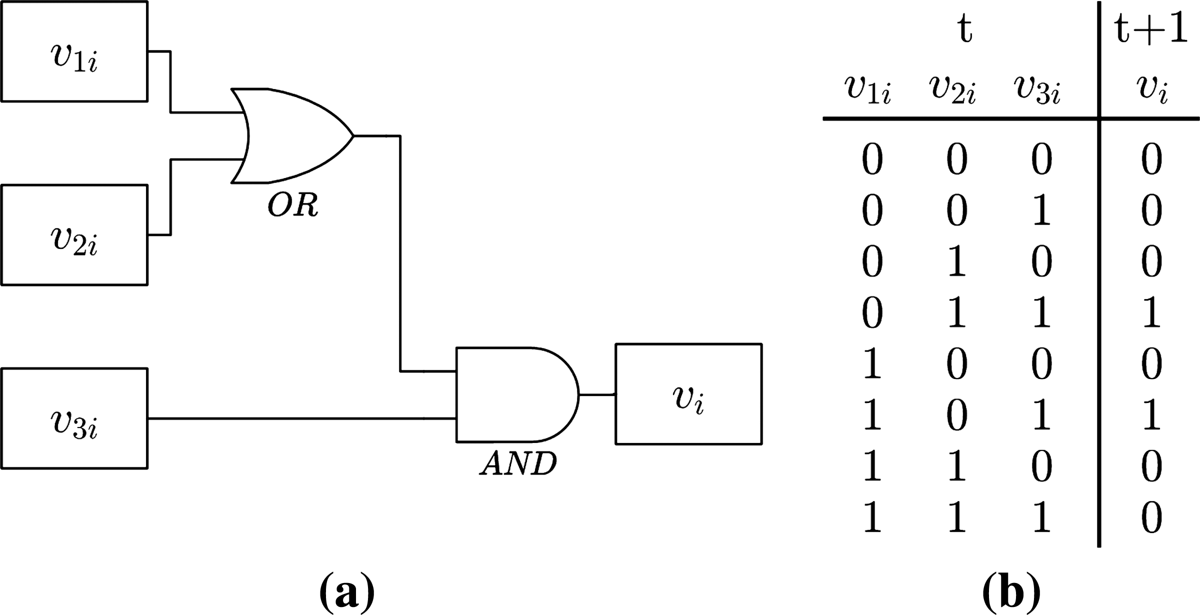
Example of a possible Boolean transfer function for a target, represented as a logic circuit (a) and as a rule table (b). The function here is defined as a mapping from the target state at time t to t+1, based on its predictors values at time t. This function underlies the simulation of the dynamical expression of the target v_i at t+1 based on the values of its predictors v_1i, v_2i and v_3i, (k = 3) at instant.

Each logic circuit \documentclass{aastex}\usepackage{amsbsy}\usepackage{amsfonts}\usepackage{amssymb}\usepackage{bm}\usepackage{mathrsfs}\usepackage{pifont}\usepackage{stmaryrd}\usepackage{textcomp}\usepackage{portland,xspace}\usepackage{amsmath,amsxtra}\pagestyle{empty}\DeclareMathSizes{10}{9}{7}{6} \begin{document} $$\psi_i , i = 1 , \ldots , n$$\end{document} is created by randomly chosen Boolean functions from a discrete set F. There are \documentclass{aastex}\usepackage{amsbsy}\usepackage{amsfonts}\usepackage{amssymb}\usepackage{bm}\usepackage{mathrsfs}\usepackage{pifont}\usepackage{stmaryrd}\usepackage{textcomp}\usepackage{portland,xspace}\usepackage{amsmath,amsxtra}\pagestyle{empty}\DeclareMathSizes{10}{9}{7}{6} \begin{document} $$2^{2^{k}}$$\end{document} possible Boolean functions, i.e., if a target has two predictors, there are \documentclass{aastex}\usepackage{amsbsy}\usepackage{amsfonts}\usepackage{amssymb}\usepackage{bm}\usepackage{mathrsfs}\usepackage{pifont}\usepackage{stmaryrd}\usepackage{textcomp}\usepackage{portland,xspace}\usepackage{amsmath,amsxtra}\pagestyle{empty}\DeclareMathSizes{10}{9}{7}{6} \begin{document} $$2^{2^{2}} = 16$$\end{document} possible Boolean functions that can be used to represent the functional dependency between the target and its predictors. On the other hand, there are Boolean functions that do not depend on one or more predictors, such as contradiction (always false) and tautology (always true), to name but a few. In the current work, only Boolean functions that depend on all predictors are considered in the discrete set F (Liang et al., 1998), once the computational methods can only detect predictors that actually participate of the signal generation.

2.1.3. Simulation of time series expression profiles

Once the network topology and the transition functions have been defined, it is possible to simulate temporal signal dynamics (expressions) by using the probabilistic transition functions. In the current work, the dynamics of an AGN is based on finite dynamical systems, discrete in time and finite in its states, given by: \documentclass{aastex}\usepackage{amsbsy}\usepackage{amsfonts}\usepackage{amssymb}\usepackage{bm}\usepackage{mathrsfs}\usepackage{pifont}\usepackage{stmaryrd}\usepackage{textcomp}\usepackage{portland,xspace}\usepackage{amsmath,amsxtra}\pagestyle{empty}\DeclareMathSizes{10}{9}{7}{6} \begin{document} \begin{align*}\vec{s} ( t + 1 ) = \Psi ( \vec{s} (t)), \tag{5}\end{align*}\end{document}

where \documentclass{aastex}\usepackage{amsbsy}\usepackage{amsfonts}\usepackage{amssymb}\usepackage{bm}\usepackage{mathrsfs}\usepackage{pifont}\usepackage{stmaryrd}\usepackage{textcomp}\usepackage{portland,xspace}\usepackage{amsmath,amsxtra}\pagestyle{empty}\DeclareMathSizes{10}{9}{7}{6} \begin{document} $$s ( t ) \in D^n , \forall \ t \ge 0$$\end{document} .

The dynamics is determined by three elements, (a) an arbitrary initial state \documentclass{aastex}\usepackage{amsbsy}\usepackage{amsfonts}\usepackage{amssymb}\usepackage{bm}\usepackage{mathrsfs}\usepackage{pifont}\usepackage{stmaryrd}\usepackage{textcomp}\usepackage{portland,xspace}\usepackage{amsmath,amsxtra}\pagestyle{empty}\DeclareMathSizes{10}{9}{7}{6} \begin{document} $$\vec{s}_j ( t ) = \{ v_1 = 0 , v_2 = 1 , \ldots , v_n = 1 \} $$\end{document} at time t, (b) the transition functions Ψ, and (c) the number of instants of time T, such that \documentclass{aastex}\usepackage{amsbsy}\usepackage{amsfonts}\usepackage{amssymb}\usepackage{bm}\usepackage{mathrsfs}\usepackage{pifont}\usepackage{stmaryrd}\usepackage{textcomp}\usepackage{portland,xspace}\usepackage{amsmath,amsxtra}\pagestyle{empty}\DeclareMathSizes{10}{9}{7}{6} \begin{document} $$\vec{s}_u ( t + 1 ) = \Psi ( \vec{s}_j ( t ) ) , \vec{s}_u , \vec{s}_j \in S , ( t = 0 , 1 , \ldots , T - 1 )$$\end{document} . These parameters define the signal generation of an AGN, and consequently the trajectories in its state transition graph (Fig. 4).

FIG. 4.

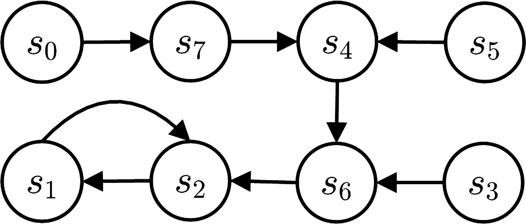
An example of the state transition graph for an AGN with n = 3$. Each vertex represents a network state. One example of trajectory is the path formed by the states S₅_, S₄, S₆, S₂.

In the AGN context, the trajectory is the path followed by a network in its state transition space, given an initial state. The state space of an AGN can be very large, but it is finite and defined by \documentclass{aastex}\usepackage{amsbsy}\usepackage{amsfonts}\usepackage{amssymb}\usepackage{bm}\usepackage{mathrsfs}\usepackage{pifont}\usepackage{stmaryrd}\usepackage{textcomp}\usepackage{portland,xspace}\usepackage{amsmath,amsxtra}\pagestyle{empty}\DeclareMathSizes{10}{9}{7}{6} \begin{document} $$S = \{\vec{s}_1 , \vec{s}_2 , \ldots , \vec{s}_z \} , z = 2^n$$\end{document} . Figure 4 shows an example of the state transition graph for an AGN with n = 3. One example of a trajectory is the path formed by the states S₅, S₄, S₆, S₂, S₁.

In summary, the dynamics of the AGN is modeled by applying the Boolean transfer functions while considering a given network initial state at time t₀ and the number of instants of time T (number of temporal expressions needed). The target state at time \documentclass{aastex}\usepackage{amsbsy}\usepackage{amsfonts}\usepackage{amssymb}\usepackage{bm}\usepackage{mathrsfs}\usepackage{pifont}\usepackage{stmaryrd}\usepackage{textcomp}\usepackage{portland,xspace}\usepackage{amsmath,amsxtra}\pagestyle{empty}\DeclareMathSizes{10}{9}{7}{6} \begin{document} $$t_i , i = 0 , 1 , 2 , \ldots , T - 1$$\end{document} is obtained by observing its predictors values at t_i and applying its respective Boolean transfer function \documentclass{aastex}\usepackage{amsbsy}\usepackage{amsfonts}\usepackage{amssymb}\usepackage{bm}\usepackage{mathrsfs}\usepackage{pifont}\usepackage{stmaryrd}\usepackage{textcomp}\usepackage{portland,xspace}\usepackage{amsmath,amsxtra}\pagestyle{empty}\DeclareMathSizes{10}{9}{7}{6} \begin{document} $$v_i ( t + 1 ) = \psi_i ( v_{1i} ( t ) , v_{2i} ( t ) , \ldots , v_{ki} ( t ) ) $$\end{document} , which is randomly chosen among its possible Boolean functions. As a result, we have the simulated temporal data along T instants of time (signal size), which can be used for the network identification procedure presented in the following section.

2.2. Network identification

The network identification method adopted in this work is based on the probabilistic genetic network (PGN) (Barrera et al., 2007). In this method the network identification process is modeled as a series of feature selection problems, one for each gene.

The network identification starts by selecting a target gene Y. A search is performed in order to determine the subset of genes (predictors) X ⊆ V yielding the best prediction of the Y value in the next instant of time. In other words, the time series determined by gene expressions are used to build a table of conditional probabilities of the classes Y given the patterns X that minimizes the mean conditional entropy given by Equation (6). The classes are defined by the target values at time t + 1, while the patterns are defined by the values of the predictors at time t.

As defined in (Lopes et al., 2008b) the mean conditional entropy of Y given all the possible instances \documentclass{aastex}\usepackage{amsbsy}\usepackage{amsfonts}\usepackage{amssymb}\usepackage{bm}\usepackage{mathrsfs}\usepackage{pifont}\usepackage{stmaryrd}\usepackage{textcomp}\usepackage{portland,xspace}\usepackage{amsmath,amsxtra}\pagestyle{empty}\DeclareMathSizes{10}{9}{7}{6} \begin{document} $${ \bf x} \in { \bf X}$$\end{document} is given by: \documentclass{aastex}\usepackage{amsbsy}\usepackage{amsfonts}\usepackage{amssymb}\usepackage{bm}\usepackage{mathrsfs}\usepackage{pifont}\usepackage{stmaryrd}\usepackage{textcomp}\usepackage{portland,xspace}\usepackage{amsmath,amsxtra}\pagestyle{empty}\DeclareMathSizes{10}{9}{7}{6} \begin{document} \begin{align*}H ( Y | { \bf X} ) = \sum_{{\bf x} \in { \bf X}} P ( { \bf x} ) H ( Y | { \bf x} ) , \tag{6}\end{align*}\end{document}

where P(Y · x) is the conditional probability of Y given the observation of the instance \documentclass{aastex}\usepackage{amsbsy}\usepackage{amsfonts}\usepackage{amssymb}\usepackage{bm}\usepackage{mathrsfs}\usepackage{pifont}\usepackage{stmaryrd}\usepackage{textcomp}\usepackage{portland,xspace}\usepackage{amsmath,amsxtra}\pagestyle{empty}\DeclareMathSizes{10}{9}{7}{6} \begin{document} $${\bf x} , H ( Y | { \bf x} ) = - \sum\nolimits_{y \in Y}P ( y | {\bf x} ) \log P ( y | {\bf x})$$\end{document} . Lower values of H yield better feature subspaces, in the sense that the lower the value of H, the larger is the information gained about Y while observing X. In general, temporal expression experiments involve thousands of genes and few observations along time. In face of this limitation, the penalization of non-observed instances was adopted in the calculus of the mean conditional entropy (Martins, Jr., et al., 2006).

The non-observed instances correspond to the patterns generated by the predictors values that do not appear on the input expression dataset. These non-observed instances receive entropy values equal to H(Y). The mass probability for the non-observed instances is parameterized by α (α = 1 in the present work). This parameter is added to the absolute frequency (number of occurrences) of all possible instances. The higher the value of α, the higher is the penalization of non-observed instances. Therefore, the mean conditional entropy with this type of penalization becomes: \documentclass{aastex}\usepackage{amsbsy}\usepackage{amsfonts}\usepackage{amssymb}\usepackage{bm}\usepackage{mathrsfs}\usepackage{pifont}\usepackage{stmaryrd}\usepackage{textcomp}\usepackage{portland,xspace}\usepackage{amsmath,amsxtra}\pagestyle{empty}\DeclareMathSizes{10}{9}{7}{6} \begin{document} \begin{align*}H ( Y | { \bf X } ) = \frac { \alpha ( M - N ) H ( Y )} {\alpha M + T} + \frac {\sum_{i = 1}^N (f_i + \alpha ) H (Y | {\bf X } = {\bf x }_{\bf i})}{\alpha M + T} , \tag { 7 }\end{align*}\end{document}

where M is the number of possible instances of the feature vector X, N is the number of actually observed instances (so, the number of non-observed instances is given by M − N), f_i is the absolute frequency (number of observations) of x_i, and T is the number of temporal samples.

The search space is normally very large, so that an exhaustive search cannot be performed. In our approach, the Sequential Forward Floating Selection (SFFS) (Pudil et al., 1994) algorithm was applied for each target gene in order to select the set X that minimizes the criterion function (penalized mean conditional entropy) given by Equation (7). The selected features are taken as predictor genes for each target gene. Hence, the selected predictors are used to link the genes and thus to recover the network topology.

An open source software (Lopes et al., 2008b) implements the network identification method described above. It is applied to the simulated temporal expressions variations, presented in Section Results and Discussion, in order to recover the network topology.

The next section presents measurements extracted from the identified and from original networks in order to quantify the similarity between them. This is the proposed approach to validate the accuracy of the identification method and its ability to recover the original structure by using different network topologies and parameters variations.

2.3. Validation

The AGNs considering the complex network models were first represented in terms of their respective adjacency matrices M, such that each edge from vertex i to vertex j implies M(i, j) = 1, with M(i, j) = otherwise.

In order to quantify the similarity between two given networks (with A corresponding to the original [AGN] and B to the one identified), we adopted the similarity measurements (Dougherty, 2007) based on a confusion matrix (Webb, 2002). Considering the context of this work, each element in a confusion matrix measures how much a network inference method gets “confused” in identifying the network edges. The confusion matrix shown in Table 1 contains information about the edges of an AGN and the inferred network done by the network identification method. The entries in the confusion matrix have the following meaning in the context of this work: TN is the number of non-identified edges that are absent in the original network, FP is the number of identified edges that are absent in the original network, FN is the number of non-identified edges that are present in the original network, and TP is the number of identified edges that are present in the original network.

Table 1.

Confusion Matrix

Edge/connection	Inferred in B	Non inferred in B
Present in A	TP	FN
Absent in A	FP	TN

The measures considered in this work are widely used by inference methods and are calculated as follows: \documentclass{aastex}\usepackage{amsbsy}\usepackage{amsfonts}\usepackage{amssymb}\usepackage{bm}\usepackage{mathrsfs}\usepackage{pifont}\usepackage{stmaryrd}\usepackage{textcomp}\usepackage{portland,xspace}\usepackage{amsmath,amsxtra}\pagestyle{empty}\DeclareMathSizes{10}{9}{7}{6} \begin{document} \begin{align*} Similarity ( A , B ) & = \root { 3 } \of { PPV \cdot Specificity \cdot Sensitivity , } \\ PPV & = \frac { TP } { ( TP + FP ) } , & ( 8 ) \\ Specificity & = \frac { TN } { ( TN + FP ) } , \\ Sensitivity & = \frac { TP } { ( TP + FN ) } . \end{align*}\end{document}

The PPV (Positive Predictive Value or accuracy) and the Specificity defined by Equation 8 quantify the correct and incorrect inferred edges by observing the measures presented in Table 1. The Sensitivity quantify the edges in the original network that were not inferred. Since the PPV, Specificity and Sensitivity are not independent of each other, the similarity requires a geometric average to represent their mean. For this reason, we take into account the geometrical average given by Similarity(A, B) in Equation 8. It is important to observe that both correct and incorrect edges are taken into account by these indices, thus implying the maximum similarity to be obtained for indices values near 1.

3. Results And Discussion

This section presents the experimental results obtained by considering four distinct network architectures, which are taken into account in this work in order to analyse the importance of the network topology on the network identification methodology. The experiments were performed in order to analyse not only the networks topologies, but also to investigate the impact of recovering networks by considering the following aspects: (1) complexity in terms of average degree 〈k〉 variation; (2) signal size variation; (3) similarity recover by considering the 10% most connected genes, i.e., hubs.

For all experiments, the four network models (ER, WS, BA, and GG) were used with 100 vertices (genes). The average degree 〈k〉 varied from 1 to 5, and the number of observed instants of time (signal size) varied from 5, 10, 15, 20 to 100 in steps of 20. For each vertex v_i, three possible Boolean functions were randomly select, which would be used to determine its dynamics, such that \documentclass{aastex}\usepackage{amsbsy}\usepackage{amsfonts}\usepackage{amssymb}\usepackage{bm}\usepackage{mathrsfs}\usepackage{pifont}\usepackage{stmaryrd}\usepackage{textcomp}\usepackage{portland,xspace}\usepackage{amsmath,amsxtra}\pagestyle{empty}\DeclareMathSizes{10}{9}{7}{6} \begin{document} $$\psi_i = \{ f_j^{ ( i ) } \} , j = 1 , \ldots , l ( i ) = 3$$\end{document} and its probabilities \documentclass{aastex}\usepackage{amsbsy}\usepackage{amsfonts}\usepackage{amssymb}\usepackage{bm}\usepackage{mathrsfs}\usepackage{pifont}\usepackage{stmaryrd}\usepackage{textcomp}\usepackage{portland,xspace}\usepackage{amsmath,amsxtra}\pagestyle{empty}\DeclareMathSizes{10}{9}{7}{6} \begin{document} $$c_1^{ ( i ) } = 0.95 , \ c_2^{ ( i ) } = 0.025 , \ c_3^{ ( i ) } = 0.025 , \ i = 1 , \ldots , 100$$\end{document} . The experimental results were obtained from 50 simulations of each network topology and 〈k〉 value.

In order to identify the networks, the simulated temporal expressions were submitted to the software (Lopes et al., 2008b) that implements the identification method described in Section 2.2. The figures presented in this section have the Similarity measure (described in Section 2.3) between AGN-based network and the identified network shown in the y-axis. In the x-axis, we have some variations in the simulated temporal expression generation, such as signal size and average degree.

The first experiment was performed in order to analyse the impact of increase the complexity in terms of average degree 〈k〉. Figure 5 presents these results by considering ER, WS, BA, and GG topologies, in which the average Similarity measure was calculated by taking into account the average results for all variations of signal size.

FIG. 5.

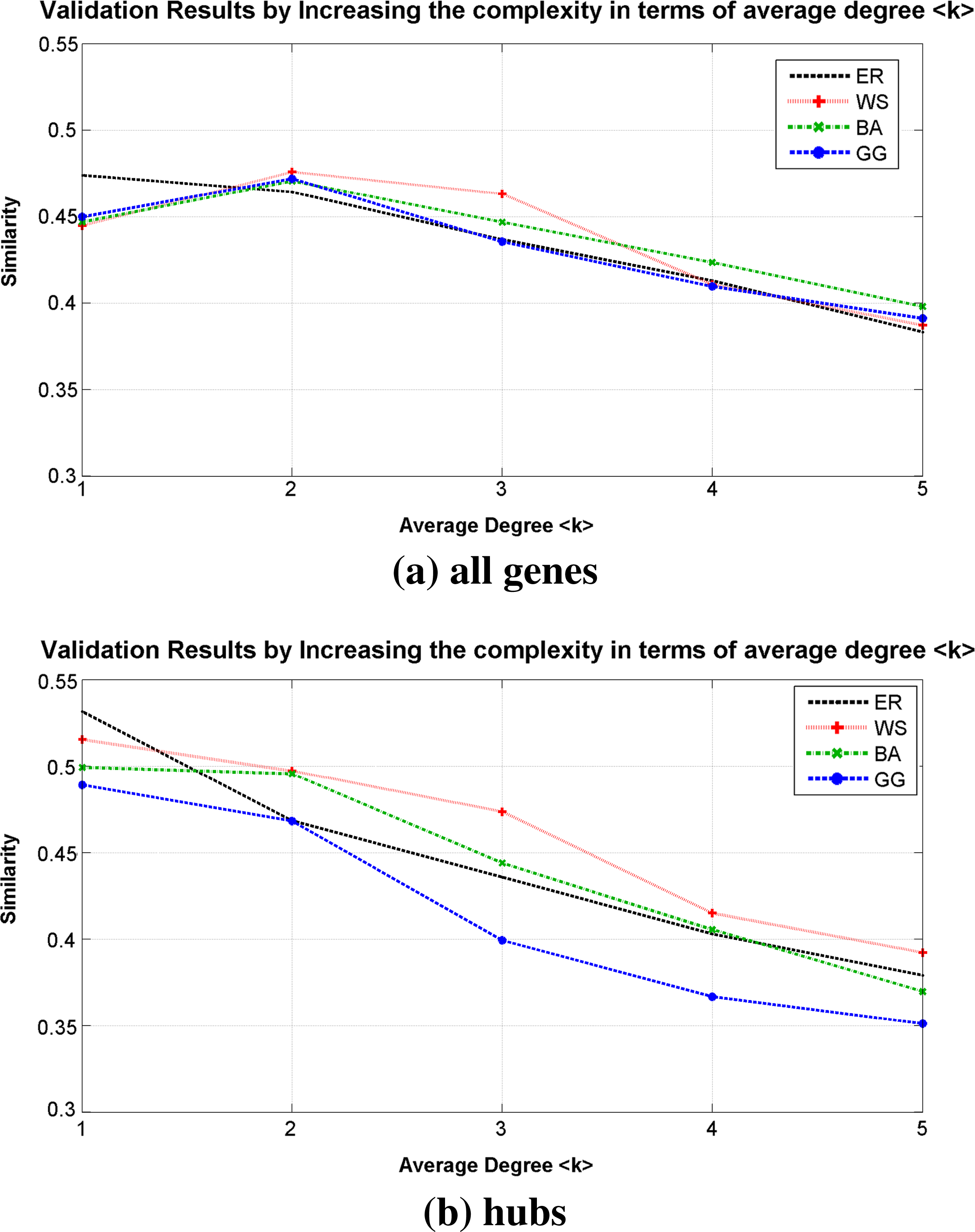
Similarity measure obtained by increasing the average degree k of edges per vertex.

It is possible to notice that, as expected, the average degree 〈k〉 is an important network component of complexity to create its dynamics, as reported by Kauffman (1969, 1993). The inference of all topologies had a decrease of Similarity with the increase of average edges per target. However, there was an improvement in results from 〈k〉 = 1 to 〈k〉 = 2 for WS, BA, and GG topologies by considering all genes. Although the network is less complex when 〈k〉 = 1, several genes may have no predictor, but the inference method found a false positive, thus reducing its similarity ratio. The same behavior does not occur with the hubs, which remained monotonically decreasing.

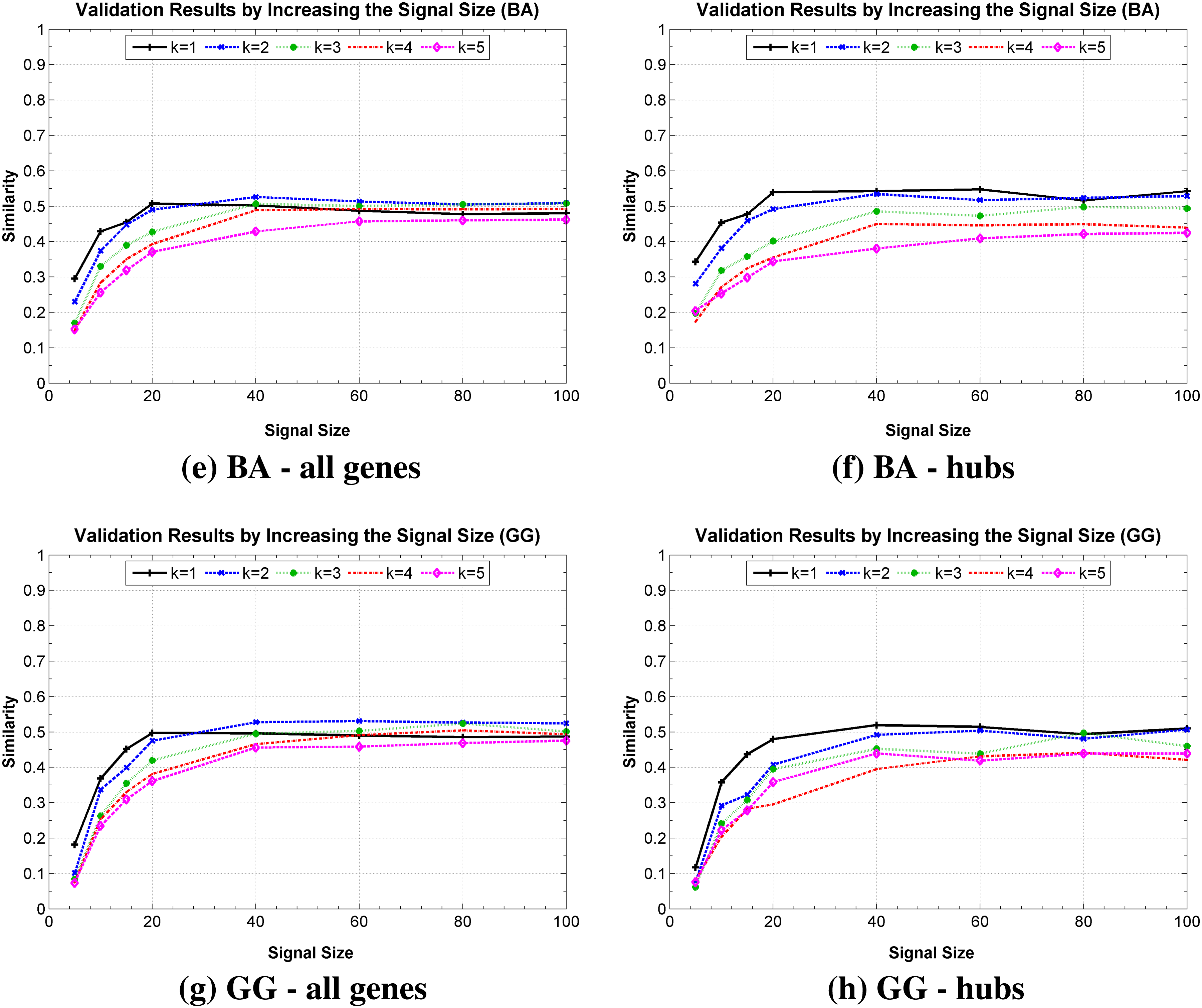
The second experiment looked at the impact of the simulated temporal expressions size on the network identification. Figure 6 presents these results by considering ER, WS, BA, and GG topologies, in which the average degree 〈k〉 was considered individually in order to observe the Similarity measure in different scales of complexity. It is possible to observe a significant improvement on the Similarity measure until approximately 20 instants of time for the four network models, indicating, as expected, that the signal size is an important factor for the proper recovery of the network. However, it is important to observe that for these networks, which involve 2¹⁰⁰ possible states, it was possible to recover in average more than 50% of the network Similarity after only 40 observations, even considering the hubs. These results show an important property of the inference method, which was able to get a good Similarity rate by observing few instants of time. Another important property was hubs recovery, which occur in a similar rate to other less connected genes of the network. Surprisingly, the inference method was not sensitive to the dynamics variation of network topology, presenting similar responses for different topologies.

FIG. 6.

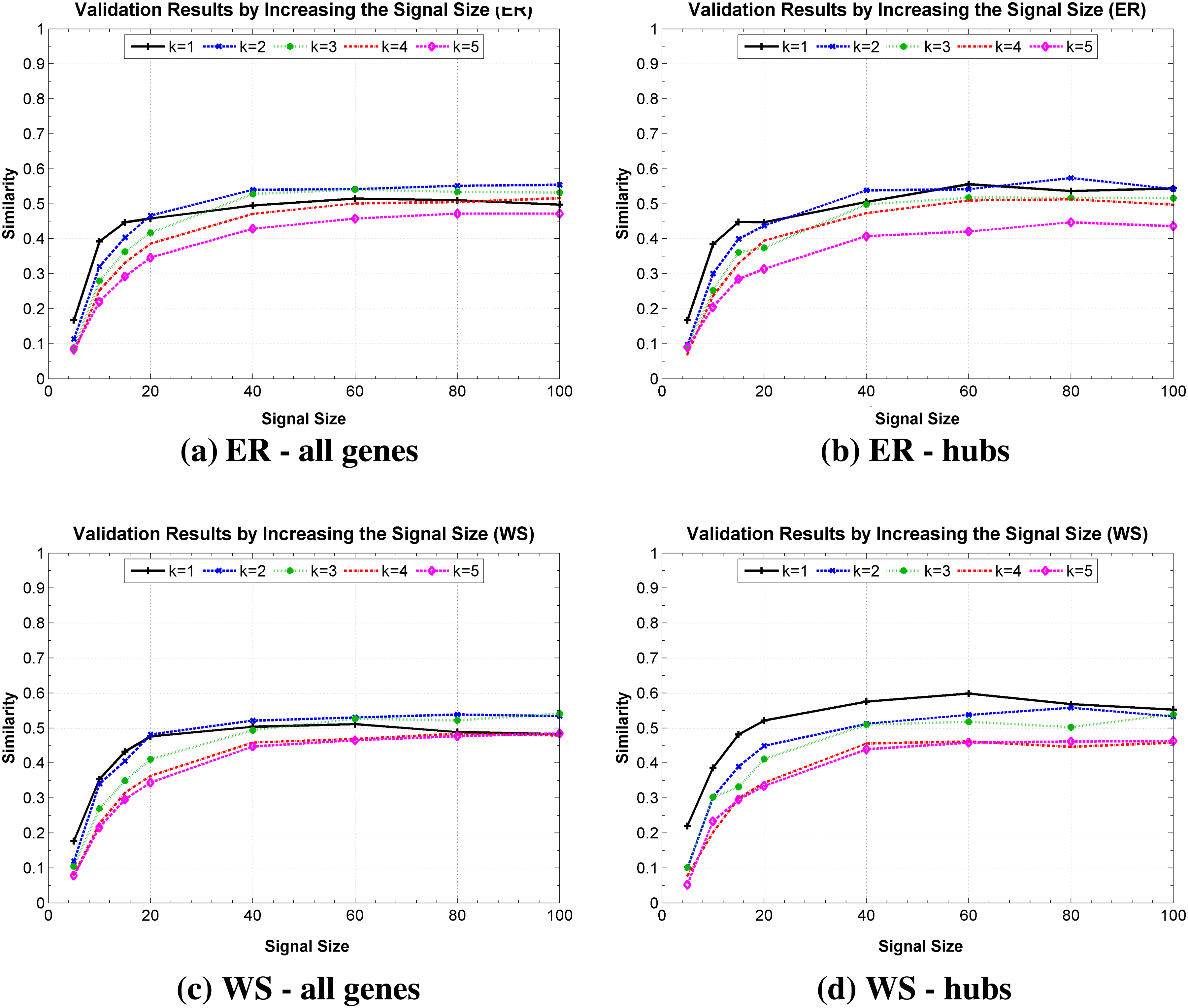
Similarly measure obtained by increasing the number of observations of the temporal expression (signal size), (a), (c), (e), and (g) by considering all genes and (b), (d), (f), and (h) just the 10% most connected genes of the network, i.e., hubs.

In order to investigate this behavior, the histograms of indegree and outdegree distributions were generated by taking into account the average (input and output edges) of the genes for all variations of signal size and average degree 〈k〉.

The experimental results, presented in Figure 7, show that the adopted methodology for the topology construction produce a balanced amount between input and output edges. On the other hand, these results confirm that the inference method produces very similar responses for all topologies, i.e., does not seem sensible to recognize different structures of relationships among genes generated by different network topologies. In addition, the outdegree distribution for inferred networks indicate that several genes are not selected as predictors, whereas some others participate of the prediction of many genes.

FIG. 7.

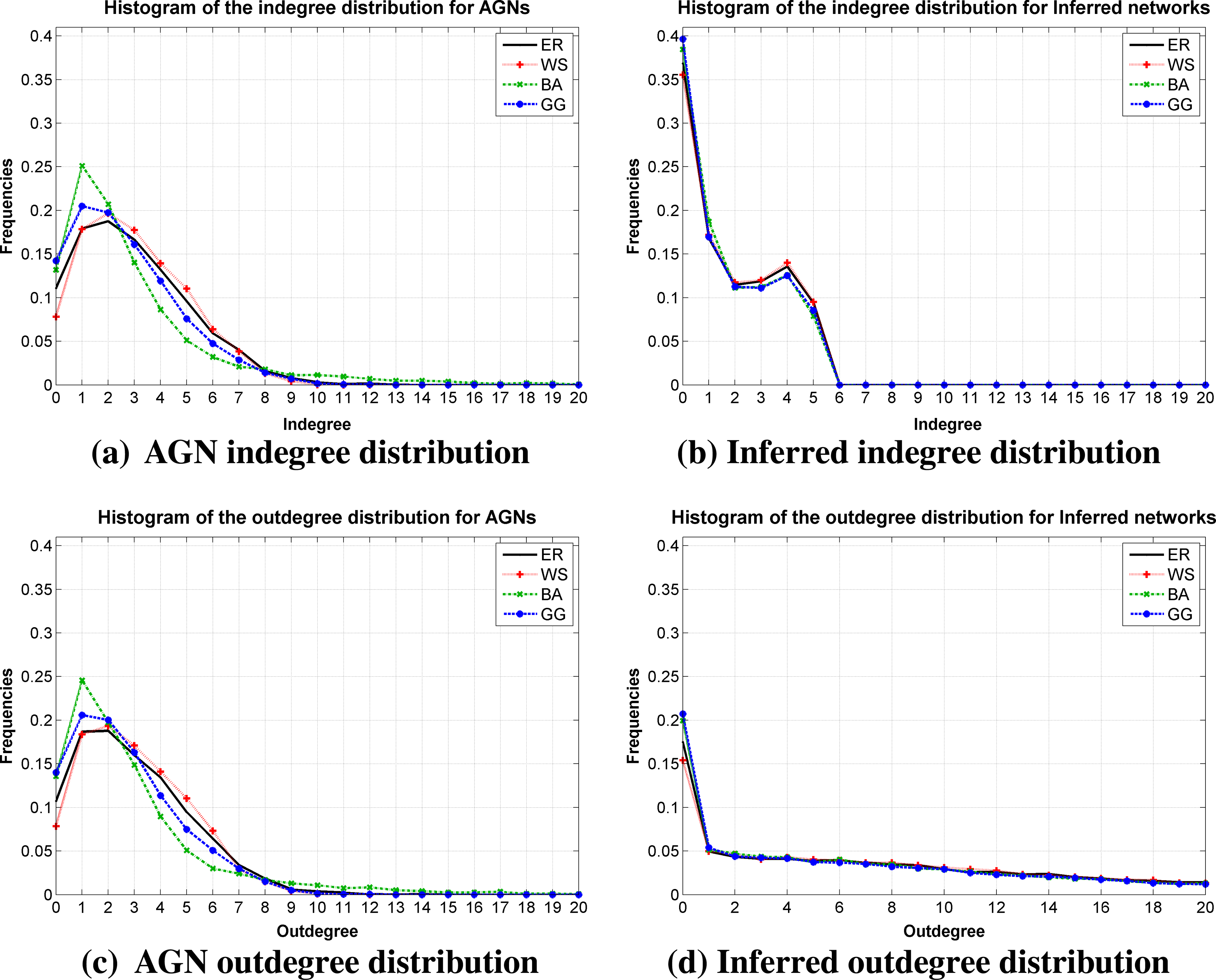
Historgram of the indegree and outdegree obtained from AGNs and inferred networks by considering the average degree distribution over all variations of signal size and average degree k.

4. Conclusion

Biological organisms respond quickly to changes in the external or internal environment, adjusting their gene expression profile. As a result, the regulatory and metabolic networks will also adjust to these changes. However, much remains to be discovered about how these modifications in the production of transcripts and proteins are linked and regulated over time. Several methods were proposed for modeling and identification of GRNs from expression profiles, but the information needed to validate the inferred networks is incomplete or unknown.

This work presented an objective approach to generate artificial gene networks, based on complex network models that define the topology and Boolean functions applied as probabilistic transition functions to simulate temporal expression profiles from it. A network identification method was applied to recover network topology from temporal expression profile, which is compared with artificial gene network by using measures of correct and incorrect inferred edges in order to validate the identified network.

The proposed framework is mainly based on only two parameters: number of vertices or “genes” n and average degree 〈k〉. There are other two parameters that guide the stochasticity of the model: the number of Boolean functions per gene l(i) and its probabilities of being used to describe the dynamics of this gene. This is done in order to consider an external stimuli on network dynamics, which would change the behavior (transition function) of the organism. Although simple, it is based on Boolean formalism that has a solid background, which was adequate for the validation of the inferred networks by identifying some properties of the evaluated method. It is important to notice that due to the adopted Boolean formalism, it is not necessary to worry about the data pre-processing, which is particularly important for inference methods based on information theory.

The proposed framework has been applied in order to investigate the behavior of the network inference method with respect to: (1) different complex network topologies (ER, WS, BA, and GG); (2) complexity in terms of average degree 〈k〉 variation; (3) signal size variation; and (4) similarity recover by considering the 10% most connected genes, i.e., hubs.

The results confirm that the average degree 〈k〉 is an important component of the network complexity and the inference method had a decrease of Similarity with the increase of average degree 〈k〉. The results indicate that the inference method was sensitive to network topology only for average degree 〈k〉 variation. The improvement observed from 〈k〉 = 1 to 〈k〉 = 2 occurs just for WS, BA and GG topologies, which present some level of organization on its edges.

The signal size is an important factor for correct inference of gene connections. This result was expected as a consequence of the increase of the signal size, thus allowing more observations. However, the inference method was able to recover more than 50% of the network Similarity after only 40 observations from a a state space of size 2¹⁰⁰, presenting very good results. This Similarity rate was very similar to the 10% most connected genes (hubs). These results indicate a good property for the inference method, by identifying genes which are determined by the composition of Boolean functions from more predictors, generating more sophisticated boolean combinations and being more difficult to identify.

Surprisingly, the adopted inference method showed similar results for all tested complex network topologies, which draws attention to the topology that has been applied to characterize biological networks (Watts and Strogatz, 1998; Stuart et al., 2003; Barabási and Oltvai, 2004; Carroll et al., 2004; Albert, 2005). The results indicate that the network topology could be an important aspect to be explored as prior information by the inference methods in order to improve its accuracy.

The network identification method was found to be robust even in the presence of some perturbations in the temporal signal, implied by the stochasticity in the application of transition functions.

A possible extension of the present work is to implement complex network measurements and then to analyse not only global measures but also local network measures (da F. Costa et al., 2007), i.e., measures based on individual genes or respective subsets. In addition, it is possible to consider similarity measures that explore other network properties (Dougherty, 2007). The application of the proposed framework in order to evaluate large-scale networks or other network inference method is direct. Finally, an open source software that implements the proposed framework is available at http://code.google.com/p/jagn/.

Footnotes

Acknowledgments

L. F. C. thanks CNPq (301303/06-1) and FAPESP (05/00587-5) for sponsorship. This work was supported by FAPESP, CNPq, and CAPES.

Disclosure Statement

No competing financial interests exist.

References

Albert

, Thakar

, Li

et al. 2008. Boolean network simulations for life scientists. Source Code Biol. Med., 3:16.

Albert

2005. Scale-free networks in cell biology. J. Cell. Sci., 118:4947–4957.

Albert

, Barabási

A.L.

2002. Statistical mechanics of complex networks. Rev. Mod. Phys., 74:47–97.

Albert

, Othmer

H.G.

2003. The topology of the regulatory interactions predicts the expression pattern of the segment polarity genes in drosophila melanogaster. J. Theor. Biol., 223:1–18.

Bansal

, Belcastro

, Ambesi-Impiombato

et al. 2007. How to infer gene networks from expression profiles. Mol. Syst. Biol., 3:78.

Barabási

A.L.

, Albert

1999. Emergence of scaling in random networks. Science, 286:509–512.

Barabási

A.L.

, Oltvai

2004. Network biology: understanding the cell's functional organization. Nat. Rev. Genet., 5:101–113.

Barrera

, Cesar

R.M.

Jr. , Martins

D.C.

Jr.

et al. 2007. Constructing probabilistic genetic networks of Plasmodium falciparum, from dynamical expression signals of the intraerythrocytic development cycle, 11–26. Methods of Microarray Data Analysis V. Springer-Verlag: New York.

Boccaletti

, Latora

, Moreno

et al. 2006. Complex networks: structure and dynamics. Physics Rep., 424:175–308.

10.

Carroll

S.B.

, Grenier

J.K.

, Weatherbee

S.D.

2004. From DNA to Diversity: Molecular Genetics and the Evolution of Animal Design, 2nd. Wiley-Blackwell: New York.

11.

, Costa

, Rodrigues

F.A.

, Cristino

A.S.

2008. Complex networks: the key to systems biology. Genet. Mol. Biol., 31:591–601.

12.

, Costa

, Rodrigues

F.A.

, Travieso

et al. 2007. Characterization of complex networks: a survey of measurements. Adv. Physics, 56:167–242.

13.

Davidich

M.I.

, Bornholdt

2008. Boolean network model predicts cell cycle sequence of fission yeast. PLoS ONE, 3:e1672.

14.

de Jong

2002. Modeling and simulation of genetic regulatory systems: a literature review. J. Comput. Biol., 9:67–103.

15.

de Jong

, Geiselmann

, Hernandez

et al. 2003. Genetic Network Analyzer: qualitative simulation of genetic regulatory networks. Bioinformatics, 19:336–344.

16.

de la Fuente

, Bing

, Hoeschele

et al. 2004. Discovery of meaningful associations in genomic data using partial correlation coefficients. Bioinformatics, 20:3565–3574.

17.

D'Haeseleer

, Liang

, Somogyi

1999. Gene expression data analysis and modeling. Proc. Pac. Symp. Biocomput. citeseer.ist.psu.edu/333426.html. 2011 February 1.

18.

D'haeseleer

, Liang

, Somogyi

2000. Genetic network inference: from co-expression clustering to reverse engineering. Bioinformatics, 16:707–726.

19.

Dougherty

E.R.

2007. Validation of inference procedures for gene regulatory networks. Curr. Genom., 8:351–359.

20.

DREAM. 2009. Dream: dialogue for reverse engineering assessments and methods. http://wiki.c2b2.columbia.edu/dream/. 2011 February 1.

21.

Erdös

, Rényi

1959. On random graphs. Publ. Math. Debrecen, 6:290–297.

22.

Espinosa-Soto

, Padilla-Longoria

, Alvarez-Buylla

E.R.

2004. A gene regulatory network model for cell-fate determination during Arabidopsis thaliana flower development that is robust and recovers experimental gene expression profiles. Plant Cell, 16:2923–2939.

23.

Farkas

I.J.

, Jeong

, Vicsek

et al. 2003. The topology of the transcription regulatory network in the yeast, Saccharomyces cerevisiae. Phys. A Stat. Mech. Appl., 318:601–612.

24.

Faure

, Naldi

, Chaouiya

et al. 2006. Dynamical analysis of a generic Boolean model for the control of the mammalian cell cycle. Bioinformatics, 22:e124–131.

25.

Gastner

M.T.

, Newman

M.E.J.

2006. The spatial structure of networks. Eur. Phys. J. B Condensed Matter, 49:247–252.

26.

Guelzim

, Bottani

, Bourgine

et al. 2002. Topological and causal structure of the yeast transcriptional regulatory network. Nat. Genet., 31:60–63.

27.

Haynes

B.C.

, Brent

M.R.

2009. Benchmarking regulatory network reconstruction with GRENDEL. Bioinformatics, 25:801–807.

28.

Hecker

, Lambeck

, Toepfer

et al. 2009. Gene regulatory network inference: data integration in dynamic models—A review. Biosystems, 96:86–103.

29.

Hickman

G.J.

, Hodgman

T.C.

2009. Inference of gene regulatory networks using Boolean-network inference methods. J. Bioinform. Comput. Biol., 7:1013–1029.

30.

Karlebach

, Shamir

2008. Modelling and analysis of gene regulatory networks. Nat. Rev. Mol. Cell. Biol., 9:770–780.

31.

Kauffman

, Peterson

, Samuelsson

et al. 2003. Random Boolean network models and the yeast transcriptional network. Proc. Natl. Acad. Sci. USA, 100:14796–14799.

32.

Kauffman

S.A.

1969. Metabolic stability and epigenesis in randomly constructed genetic nets. J. Theor. Biol., 22:437–467.

33.

Kauffman

S.A.

1993. The Origins of Order: Self-Organization and Selection in Evolution. Oxford University Press: New York.

34.

Klamt

, Saez-Rodriguez

, Gilles

2007. Structural and functional analysis of cellular networks with cellnetanalyzer. BMC Syst. Biol., 1:2.

35.

, Long

, Lu

et al. 2004. The yeast cell-cycle network is robustly designed. Proc. Natl. Acad. Sci. USA, 101:4781–4786.

36.

L.M.

, Lu

H.H.S.

2005. Explore biological pathways from noisy array data by directed acyclic boolean networks. J. Comput. Biol., 12:170–185.

37.

, Assmann

S.M.

, Albert

2006. Predicting essential components of signal transduction networks: a dynamic model of guard cell abscisic acid signaling. PLoS Biol., 4:e312.

38.

Liang

, Fuhrman

, Somogyi

1998. Reveal: a general reverse engineering algorithm for inference of genetic network architectures. Proc. Pac. Symp. Biocomput., 18–29.

39.

Lopes

F.M.

, Cesar

R.M.

Jr. , da

, Costa

2008a. AGN simulation and validation model. Lect. Notes Bioinform., 5167:169–173.

40.

Lopes

F.M.

, Martins

D.C.

Jr. , Cesar

R.M.

Jr.

2008b. Feature selection environment for genomic applications. BMC Bioinform., 9:451.

41.

Lopes

F.M.

, Martins

D.C.

Jr. , Cesar

R.M.

Jr.

2009. Comparative study of GRNs inference methods based on feature selection by mutual information. Proc. GENSIPS, 2009; 1–4.

42.

Martins

D.C.

Jr. , Cesar

R.M.

Jr. , Barrera

2006. W-operator window design by minimization of mean conditional entropy. Pattern Anal. Appl., 9:139–153.

43.

Mendes

, Sha

, Ye

2003. Artificial gene networks for objective comparison of analysis algorithms. Bioinformatics, 19:122ii–129ii.

44.

Narasimhan

, Rengaswamy

, Vadigepalli

2009. Structural properties of gene regulatory networks: definitions and connections. IEEE/ACM Trans. Comput. Biol. Bioinform., 6:158–170.

45.

Nelson

D.L.

, Cox

M.M.

2004. Lehninger Principles of Biochemistry, 4th. W.H. Freeman: New York.

46.

Newman

M.E.J.

2003. The structure and function of complex networks. SIAM Rev., 45:167–256.

47.

Pearl

1988. Probabilistic Reasoning in Intelligent Systems: Networks of Plausible Inference. Morgan Kaufmann: New York.

48.

Pudil

, Novovičová

, Kittler

1994. Floating search methods in feature-selection. Pattern Recogn. Lett., 15:1119–1125.

49.

Quayle

, Bullock

2006. Modelling the evolution of genetic regulatory networks. J. Theor. Biol., 238:737–753.

50.

Sánchez

, Thieffry

2001. A logical analysis of the drosophila gap-gene system. J. Theor. Biol., 211:115–141.

51.

Schllit

, Brazma

2007. Current approaches to gene regulatory network modelling. BMC Bioinform., 8:S9.

52.

Serra

, Villani

, Semeria

2004. Genetic network models and statistical properties of gene expression data in knock-out experiments. J. Theor. Biol., 227:149–157.

53.

Shmulevich

, Dougherty

E.R.

2007. Genomic Signal Processing. Princeton University Press: Princeton, NJ.

54.

Shmulevich

, Dougherty

E.R.

, Kim

et al. 2002a. Probabilistic Boolean networks: a rule-based uncertainty model for gene regulatory networks. Bioinformatics, 18:261–274.

55.

Shmulevich

, Dougherty

E.R.

, Zhang

2002b. From Boolean to probabilistic Boolean networks as models of genetic regulatory networks. Proc. IEEE, 90:1778–1792.

56.

Shmulevich

, Kauffman

S.A.

, Aldana

2005. Eukaryotic cells are dynamically ordered or critical but not chaotic. Proc. Natl. Acad. Sci. USA, 102:13439–13444.

57.

Soranzo

, Bianconi

, Altafini

2007. Comparing association network algorithms for reverse engineering of large-scale gene regulatory networks. Bioinformatics, 23:1640–1647.

58.

Stuart

J.M.

, Segal

, Koller

et al. 2003. A gene-coexpression network for global discovery of conserved genetic modules. Science, 302:249–255.

59.

Styczynski

M.P.

, Stephanopoulos

2005. Overview of computational methods for the inference of gene regulatory networks. Comput. Chem. Eng., 29:519–534.

60.

Van den Bulcke

, Van Leemput

, Naudts

et al. 2006. Syntren: a generator of synthetic gene expression data for design and analysis of structure learning algorithms. BMC Bioinform., 7:43.

61.

Wahde

, Hertz

2000. Coarse-grained reverse engineering of genetic regulatory networks. Biosystems, 55:129–136.

62.

Wang

, Gerstein

, Snyder

2009. RNA-Seq: a revolutionary tool for transcriptomics. Nat. Rev. Genet., 10:57–63.

63.

Watts

D.J.

, Strogatz

S.H.

1998. Collective dynamics of small-world networks. Nature, 393:440–442.

64.

Webb

A.R.

2002. Statistical Pattern Recognition, 2nd. John Willey & Sons: New York.