EDAR: An Efficient Error Detection and Removal Algorithm for Next Generation Sequencing Data

Abstract

Genomic sequencing techniques introduce experimental errors into reads which can mislead sequence assembly efforts and complicate the diagnostic process. Here we present a method for detecting and removing sequencing errors from reads generated in genomic shotgun sequencing projects prior to sequence assembly. For each input read, the set of all length k substrings (k-mers) it contains are calculated. The read is evaluated based on the frequency with which each k-mer occurs in the complete data set (k-count). For each read, k-mers are clustered using the variable-bandwidth mean-shift algorithm. Based on the k-count of the cluster center, clusters are classified as error regions or non-error regions. For the 23 real and simulated data sets tested (454 and Solexa), our algorithm detected error regions that cover 99% of all errors. A heuristic algorithm is then applied to detect the location of errors in each putative error region. A read is corrected by removing the errors, thereby creating two or more smaller, error-free read fragments. After performing error removal, the error-rate for all data sets tested decreased (∼35-fold reduction, on average). EDAR has comparable accuracy to methods that correct rather than remove errors and when the error rate is greater than 3% for simulated data sets, it performs better. The performance of the Velvet assembler is generally better with error-removed data. However, for short reads, splitting at the location of errors can be problematic. Following error detection with error correction, rather than removal, may improve the assembly results.

Introduction

Next-generation sequencing (NGS) techniques make it possible to generate orders of magnitude more sequence information at substantially less cost than with traditional Sanger sequencing (ten Bosch and Grody, 2008; Schuster, 2008). Currently, four main NGS platforms are available for commercial use. They are the 454 Genome Sequencer FLX, Illumina Genome Analyzer (Solexa), ABI SOLiD System, and Helicos Heliscope (ten Bosch and Grody, 2008). These NGS platforms can generate from 0.1G up to 10G base pairs in just one instrument run (ten Bosch and Grody, 2008), with each read ranging from 25 base pairs (bps) to around 400 bps long. These sequencing technologies have been used in many applications, including re-sequencing of whole genomes using reference genomes as a template (Hiller et al., 2008), as well as de novo sequencing (Chaisson and Pevzner, 2008; Reinhardt, 2009).

One drawback of the new sequencing techniques is that their sequencing accuracies are much lower than traditional Sanger sequencing, where base-calling accuracy is around 0.01errors/kb (Eriksson, 2008). For some NGS platforms (e.g., 454), the number of errors increases dramatically near the ends of reads, making these end regions unsuitable for sequence assembly (Chaisson et al., 2009). Efficient error-correction algorithms, especially those robust to high error rates, are crucial in helping eliminate low-quality reads/bases to improve the data quality and facilitate the assembly process.

There are two common algorithmic approaches used for genome assembly: overlap-contig-consensus (OCC) and de Bruijn graph construction. The OCC approach calculates overlaps between all pairs of reads and then combines overlapping reads to form larger contigs. These contigs are then aligned to generate consensus sequences. This approach is used by several assemblers, including the Celera Assembler (Myers et al., 2000), Arachne (Batzoglou et al., 2002), Atlas (Havlak et al., 2004), CABOG (Miller et al., 2008), and Edena (Hernandez et al., 2008). The de Bruijn graph approach builds a de Bruijn graph on k-mers (k-base-long sequence) from the input reads and traverses graph edges to generate assembly. Such an algorithm was initially used by the EULER-DB assembler (Pevzner et al., 2001) and now forms the basis of the EULER-SR (Chaisson and Pevzner, 2008), ALLPATHS (Butler et al., 2008), and Velvet (Zerbino and Birney, 2008) assemblers. The OCC approach is more useful for assembly of longer reads, while de Bruijn graph methods have become more popular for assembly of next-generation short-read data. On the other hand, the de Bruijn graph approach is very sensitive to erroneous reads. These erroneous reads dramatically increase the complexity of the graph, making the assembly effort more difficult. In this work, we seek to improve sequence data quality through improvements in error detection and removal.

In recent years, the error-correction problem has attracted much interest. Three main approaches to error detection/correction have been suggested. The first method begins with a multiple sequence alignment of each read and its overlapping reads (Tammi et al., 2003; Gajer et al., 2004). For each position in the alignment, bases appearing less frequently are considered errors. However, with short read data from next-generation sequencers, false overlaps are common and this method may result in incorrect assignment of errors. The second method performs data correction based on the structure of a de Bruijn graph built from input reads. In this approach, errors are removed based on specific graph structures, such as tips (short dead-end paths in the graph), bubbles (multiple paths between two nodes), and paths with low multiplicity. This is the method utilized by Velvet (Zerbino and Birney, 2008). The main bottleneck of these algorithms is the memory usage required for graph construction, particularly for high coverage sequencing data containing sequencing errors.

In the third approach, read data are pre-processed before any attempt at assembly is made. This is the strategy employed by the EULER-DB, EULER-SR (Pevzner et al., 2001; Chaisson et al., 2004, 2009; Chaisson and Pevzner, 2008), and ALLPATH (Butler et al., 2008) assemblers. In these assemblers, a threshold k-count, M, is defined to distinguish k-mers that are very likely to contain errors (“weak” k-mers) and k-mers that are very likely to be correct (“strong” k-mers). For each read in the input data sets, the minimum number of changes is made to “weak” k-mers so that all k-mers on that read become “strong.” Optimization methods (Chaisson et al., 2004) have been applied in order to improve the speed and capacity of the algorithm. However the performance will be affected as the number of errors on each read or the length of each read is increased (Chaisson et al., 2004). With this approach, it is also possible to introduce new “errors” into the data during the process of changing “weak” k-mers into “strong” k-mers (Pevzner et al., 2001).

We report here a novel error correction algorithm, EDAR, for processing read data prior to sequence assembly. Our algorithm is mainly focused on data generated from genomic shotgun sequencing techniques. EDAR does not rely on overlap identification making it more robust for short-read data. And further, EDAR's performance does not break down as the error rate increases. For each read, k-mers are clustered based on their frequency using the variable bandwidth mean-shift (VBMS) method (Comaniciu et al., 2001). The resulting clusters are categorized as error or non-error based on the mean of the cluster and an error threshold. Next the algorithm determines the most likely error bases within each error region identified. After error bases are detected, they are removed and the raw reads are split into shorter “error-free” read fragments. Since EDAR removes, rather than corrects, detected errors, it does not change input reads; all data going into the assembler comes from actual base-calls made during the sequencing process. Though there is a potential drawback in splitting already short reads into smaller fragments at putative error bases, with the high-coverage of most next-generation sequencing data, it is highly likely that the shorter reads generated by EDAR will still cover each base in the original genome sequence. This algorithm can be applied to increase the accuracy of reads for any sequencing platform.

Methods

When a read contains a single base error, up to k adjacent k-mers will contain that error, depending on the position of the error relative to the ends of the read and the error type (e.g., mutation, insertion, or deletion). Rather than classifying a k-mer as erroneous based on its coverage alone, the EDAR method includes information about the coverage of adjacent k-mers. By determining stretches of adjacent k-mers that contain an error, the location of that error can be estimated, and it can be removed.

The EDAR method consists of the following steps:

1) Pre-process raw input reads to remove those of low quality.

2) For each k-mer in the dataset, calculate the k-count (described below).

3) Normalize k-count values based on GC content (Voelkerding et al., 2009).

4) Based on the distribution of k-counts across the dataset, determine the threshold between erroneous k-mers and correct ones.

5) For each read, cluster k-mers using the variable bandwidth mean-shift method.

6) Categorize each cluster as error or non-error based on the threshold obtained from step 3, above.

7) Post-process clusters based on k-mers' locations on the read and other criteria.

8) Analyze each error region, and detect putative error bases. Remove putative error bases from each read and generate shorter read fragments.

k-Count

Let the length of a k-mer be k, and observe that a read r with length l contains (n = l – k + 1) k-mers. Let k-count C_k(i), i = 1.n, be the coverage for the k-mer starting from position i of read r. For example, if r is: ACCTG, then C₃(2) represents the number of times the 3-mer CCT occurs over all reads in the data set.

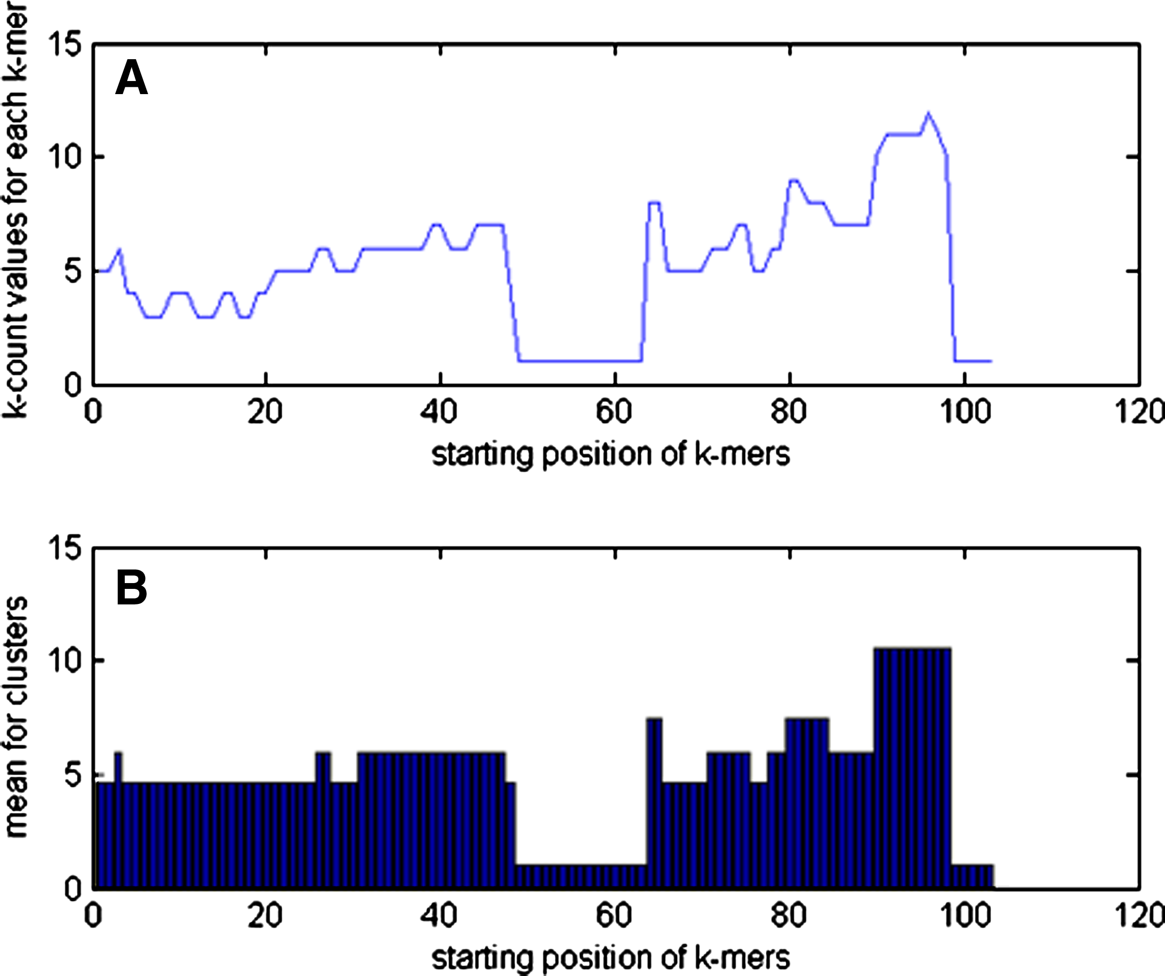
We calculate C_k for each k-mer in a read. For each read we can construct the “k-count plot” which displays the k-count value for each k-mer in that read (Fig. 1). We see from the figure that k-mers that contain errors often appear in a region with low k-count values for each point in that region; k-mers that are parts of repeats are in high k-count value regions and k-mers from unique regions or regions that contain polymorphisms have k-count values in between.

FIG. 1.

k-Count plot for a read for data with 10-fold coverage. The x-axis represents the starting position for each k-mer. The y-axis represents the k-count value for each corresponding kmer. Within a read, putative repeat regions tend to have higher coverage and errors lower coverage than unique regions.

EDAR seeks to classify k-mers as error-containing or non-error containing “regions” for each read (Fig. 1). However, these “regions” are not easy to distinguish, as even k-mers in the same region do not share exactly the same k-count values. In an idealized data set containing no sequencing errors, polymorphisms or repeats, the probability that a given base is sequenced m times follows a Poisson distribution with mean, λ, equal to the coverage for the experiment, \documentclass{aastex}\usepackage{amsbsy}\usepackage{amsfonts}\usepackage{amssymb}\usepackage{bm}\usepackage{mathrsfs}\usepackage{pifont}\usepackage{stmaryrd}\usepackage{textcomp}\usepackage{portland,xspace}\usepackage{amsmath,amsxtra}\pagestyle{empty}\DeclareMathSizes{10}{9}{7}{6}\begin{document}$$P (m) = \lambda^m \ \frac {e^{- \lambda}} {m!}$$\end{document} (Lander and Waterman, 1988). Similarly, the distribution of k-mer frequencies is expected to follow the Poisson distribution. However in a real-world sequencing project additional modes in the distribution are expected to arise due to the presence of errors, polymorphisms and repeats. We utilized the variable-bandwidth mean-shift clustering (VBMS) method to find the modes to this distribution and cluster k-count values for each read such that k-mers belonging to the same mode cluster together (Comaniciu et al., 2001).

GC-content based adjustments to k-count values

Some sequencing methods result in a coverage bias in which read coverage increases with GC-content. This is apparent particularly in data from the Solexa sequencing platform. Such bias will confuse the error detection algorithm, as low k-counts may not necessarily result from sequencing errors, and high k-counts may not be due to repeats as one would expect from un-biased data sets. For such data, we normalize k-count values prior to clustering based on their GC-contents as follows:

For each k-mer, k_i let C_k(i) be the k-count for k_i, GC(k_i) be the GC percentage for k_i, and C_k′(i) be the adjusted k-count for k_i. In addition, let cov_k be the median k-count for all k-mers and C_k,GC(ki) be the median k-count for all k-mers with the same GC percentage as k_i. Then: \documentclass{aastex}\usepackage{amsbsy}\usepackage{amsfonts}\usepackage{amssymb}\usepackage{bm}\usepackage{mathrsfs}\usepackage{pifont}\usepackage{stmaryrd}\usepackage{textcomp}\usepackage{portland,xspace}\usepackage{amsmath,amsxtra}\pagestyle{empty}\DeclareMathSizes{10}{9}{7}{6}\begin{document}\begin{align*}C_k^{\prime} (i) = C_k (i) \times \frac {{\rm cov}_k} {C_ {k , GC (k_ {i})}} \tag {1}\end{align*}\end{document}

Since error-containing k-mers will bias this calculation, a reference genome is required to accurately calculate C_k,GC(ki) and cov_k. Here we used data from Solexa sequencing of Staphylococcus aureus strain MW2. Based on these data, we calculated the ratio cov_k/C_k,GC(ki) after removing those k-mers which did not map to the reference genome.

Detecting boundaries between errors and non-error regions

In real sequencing projects, errors are inevitable, and polymorphisms and repeats make the true distribution of k-mer k-counts much more complex than a single Poisson distribution can describe. We expect that the true underlying k-count distribution is governed by a mixture model that includes exponential models for erroneous k-mers and a series of Poisson models describing polymorphisms, unique regions, and repeats. In next-generation sequencing projects, the expected coverage of each k-mer is usually high. Good separation can usually be found between the exponential distributions and high lambda Poisson distributions (Fig. 2). Currently, we are not explicitly fitting models to this distribution. We define the first minimum value (starting from left of the x-axis) in the histogram as the threshold for errors, and denote it as t_e. t_e will be utilized later to judge which cluster of k-mers contain errors. ALLPATH (Butler et al., 2008) and EULER-USR (Chaisson and Pevzner, 2008) use a similar approach.

FIG. 2.

k-Count frequency for k-mers in a simulated data set 85H09_e30. The purple line indicates a rough estimation of the boundary between the exponential models and the Poisson models. Inset: An enlargement of the figure in the region of the first minimum. The first minimum, k-count = 4, has frequency around 5000. k-mers in this region are at risk of being mislabeled as error or non-error-containing.

Cluster k-mers using the variable bandwidth mean-shift method

Within an individual read, we seek to cluster each k-mer based on its k-count. Using the Variable Bandwidth Mean-Shift (VBMS) method, each k-mer in the read is assigned to a cluster which represents a mode in the adaptive kernel density estimate (KDE).

Kernel density estimation is a non-parametric method for estimating the probability density from which a sample of data points was generated. For each read in our data set, r, we expect the KDE to produce a multimodal distribution with modes corresponding to unique regions, repeats, polymorphisms and errors (Fig. 3B). The kernel density estimate is defined as: \documentclass{aastex}\usepackage{amsbsy}\usepackage{amsfonts}\usepackage{amssymb}\usepackage{bm}\usepackage{mathrsfs}\usepackage{pifont}\usepackage{stmaryrd}\usepackage{textcomp}\usepackage{portland,xspace}\usepackage{amsmath,amsxtra}\pagestyle{empty}\DeclareMathSizes{10}{9}{7}{6}\begin{document}\begin{align*}{\hat f} (c_k) = \frac {1} {n} \sum \nolimits_ {i = 1}^{n} \frac {1} {h_i} K \left(\frac {c_k - c_k (i)} {h_i} \right) \tag {2}\end{align*}\end{document}

FIG. 3.

Clustering results for a read from a simulated data set. (A) k-Count plot for the read. (B) k-Mer clustering results using variable bandwidth mean-shift method.

where c_k(i) corresponds to the k-count for the k-mer starting at position i in read r, and h_i corresponds to the bandwith for that k-mer. The kernel K(x) is defined based on a kernel profile, such that K(x) = a k(||x||²), where a is a normalization constant. Here we use the 1-d Epanechnikov kernel with its profile defined as follows: \documentclass{aastex}\usepackage{amsbsy}\usepackage{amsfonts}\usepackage{amssymb}\usepackage{bm}\usepackage{mathrsfs}\usepackage{pifont}\usepackage{stmaryrd}\usepackage{textcomp}\usepackage{portland,xspace}\usepackage{amsmath,amsxtra}\pagestyle{empty}\DeclareMathSizes{10}{9}{7}{6}\begin{document}\begin{align*}k_E (x) = \begin{cases}1 - x \quad 0 \le x \le 1 \\ 0 \qquad \quad x > 1\end{cases} \tag {3}\end{align*}\end{document}

with the normalization constant a = 0.75.

When clustering based on the adaptive KDE, \documentclass{aastex}\usepackage{amsbsy}\usepackage{amsfonts}\usepackage{amssymb}\usepackage{bm}\usepackage{mathrsfs}\usepackage{pifont}\usepackage{stmaryrd}\usepackage{textcomp}\usepackage{portland,xspace}\usepackage{amsmath,amsxtra}\pagestyle{empty}\DeclareMathSizes{10}{9}{7}{6}\begin{document}$${\tilde f} (c_k)$$\end{document} our goal is to assign each data point to a cluster based on the mode that point would evolve to under a gradient ascent algorithm. The variable bandwidth mean-shift algorithm is a method that efficiently identifies the mode for each data point without explicitly estimating the density (Comaniciu et al., 2001). k-mers whose k-count values evolve to the same mode are clustered together (Fig. 3).

The variable bandwidth mean-shift is an iterative procedure. The mean-shift vector, m(x), is defined as follows (Comaniciu and Meer, 2002): \documentclass{aastex}\usepackage{amsbsy}\usepackage{amsfonts}\usepackage{amssymb}\usepackage{bm}\usepackage{mathrsfs}\usepackage{pifont}\usepackage{stmaryrd}\usepackage{textcomp}\usepackage{portland,xspace}\usepackage{amsmath,amsxtra}\pagestyle{empty}\DeclareMathSizes{10}{9}{7}{6}\begin{document}\begin{align*}m ({\rm x}) = \frac {\sum \nolimits_ {i = 1}^n c_k (i) g (\| \frac {{\rm x} - c_k (i)} {h_i} \|^2)} {\sum \nolimits_ {i = 1}^n g (\| \frac {{\rm x} - c_k (i)} {h_i} \|^2)} - x \tag {4}\end{align*}\end{document}

c_k(i) represent all data points in a single read. x is initialized at the location of the specific data point to be clustered. g is defined as the negative first-order derivative of k_E(x). Here for 1-d Epanechnikov kernel, g = 1 for \documentclass{aastex}\usepackage{amsbsy}\usepackage{amsfonts}\usepackage{amssymb}\usepackage{bm}\usepackage{mathrsfs}\usepackage{pifont}\usepackage{stmaryrd}\usepackage{textcomp}\usepackage{portland,xspace}\usepackage{amsmath,amsxtra}\pagestyle{empty}\DeclareMathSizes{10}{9}{7}{6}\begin{document}$$\mid {\rm x} - c_k (i) \mid \le h_i$$\end{document} , and 0 otherwise. Hence, in our problem setting, the mean-shift vector is the difference between x and the mean of those points that are within one band-width of x. If we define y₀ = x, and y_i = y_i−1 + m(y_i−1), then the sequence of y_i's converge at the mode of the KDE when m(y_i) = 0 (Comaniciu and Meer, 2002). Points that converge to the same mode as y_i form a cluster. EDAR calculates the variable bandwidth mean-shift using each point as an initial center and clusters points based on their corresponding mode.

The variable band-width h_i for each point c_k(i) was calculated as follows: \documentclass{aastex}\usepackage{amsbsy}\usepackage{amsfonts}\usepackage{amssymb}\usepackage{bm}\usepackage{mathrsfs}\usepackage{pifont}\usepackage{stmaryrd}\usepackage{textcomp}\usepackage{portland,xspace}\usepackage{amsmath,amsxtra}\pagestyle{empty}\DeclareMathSizes{10}{9}{7}{6}\begin{document}\begin{align*}h_i = h [\lambda / {\tilde f} (c_k (i))]^{1 / 2}. \tag {5}\end{align*}\end{document}

h is calculated based on the inter-quartile range R of the k-count values for all the k-mers from the read in consideration (see Equation 6) (Silverman, 1986). \documentclass{aastex}\usepackage{amsbsy}\usepackage{amsfonts}\usepackage{amssymb}\usepackage{bm}\usepackage{mathrsfs}\usepackage{pifont}\usepackage{stmaryrd}\usepackage{textcomp}\usepackage{portland,xspace}\usepackage{amsmath,amsxtra}\pagestyle{empty}\DeclareMathSizes{10}{9}{7}{6}\begin{document}\begin{align*}h = 0.79 Rn^{- 1 / 5} \tag {6}\end{align*}\end{document}

λ is the arithmetic mean of \documentclass{aastex}\usepackage{amsbsy}\usepackage{amsfonts}\usepackage{amssymb}\usepackage{bm}\usepackage{mathrsfs}\usepackage{pifont}\usepackage{stmaryrd}\usepackage{textcomp}\usepackage{portland,xspace}\usepackage{amsmath,amsxtra}\pagestyle{empty}\DeclareMathSizes{10}{9}{7}{6}\begin{document}$${\tilde f} (c_k (i))$$\end{document} over all data points \documentclass{aastex}\usepackage{amsbsy}\usepackage{amsfonts}\usepackage{amssymb}\usepackage{bm}\usepackage{mathrsfs}\usepackage{pifont}\usepackage{stmaryrd}\usepackage{textcomp}\usepackage{portland,xspace}\usepackage{amsmath,amsxtra}\pagestyle{empty}\DeclareMathSizes{10}{9}{7}{6}\begin{document}$$c_k (i)$$\end{document} . \documentclass{aastex}\usepackage{amsbsy}\usepackage{amsfonts}\usepackage{amssymb}\usepackage{bm}\usepackage{mathrsfs}\usepackage{pifont}\usepackage{stmaryrd}\usepackage{textcomp}\usepackage{portland,xspace}\usepackage{amsmath,amsxtra}\pagestyle{empty}\DeclareMathSizes{10}{9}{7}{6}\begin{document}$${\tilde f} (c_k (i))$$\end{document} is the initial kernel density estimate (also called pilot estimate) at point \documentclass{aastex}\usepackage{amsbsy}\usepackage{amsfonts}\usepackage{amssymb}\usepackage{bm}\usepackage{mathrsfs}\usepackage{pifont}\usepackage{stmaryrd}\usepackage{textcomp}\usepackage{portland,xspace}\usepackage{amsmath,amsxtra}\pagestyle{empty}\DeclareMathSizes{10}{9}{7}{6}\begin{document}$$c_k (i)$$\end{document} . For the pilot estimate, we utilized the non-adaptive (single bandwidth) Epanechnikov kernel density estimator with the initial bandwith h, defined above, to calculate the pilot estimate for each point x (Equation 7). \documentclass{aastex}\usepackage{amsbsy}\usepackage{amsfonts}\usepackage{amssymb}\usepackage{bm}\usepackage{mathrsfs}\usepackage{pifont}\usepackage{stmaryrd}\usepackage{textcomp}\usepackage{portland,xspace}\usepackage{amsmath,amsxtra}\pagestyle{empty}\DeclareMathSizes{10}{9}{7}{6}\begin{document}\begin{align*}{\tilde f} (c_k) = \frac {a} {nh} \sum_ {i = 1}^n k_E \left(\left\| \frac {c_k - c_k (i)} {h} \right\|^2 \right) \tag {7}\end{align*}\end{document}

Post-processing

Separating non-adjacent clusters

We applied 1-dimensional variable bandwidth mean-shift clustering method to cluster k-mers based on their k-count values. The position information is utilized in the post-processing step to further distinguish the clusters. In particular, let c₁, c₂, and c₁′ represent three consecutive clusters on a read, where c₁ and c₁′ are in the same cluster and c₂ in a different cluster. Since c₁ and c₁′ are not adjacent, making them in the same cluster is not appropriate as we focus on adjacent k-mers that share similar k-count values. We separate c₁ and c₁′ into two different clusters.

Joining clusters

Resulting clusters on each read are further grouped into the two categories, error or non-error, by comparing cluster means with the thresholds that were established in the threshold finding step. The resulting clusters are further post-processed. For example, error regions on sequencing reads might contain high k-count k-mers. These k-mers were not in the original DNA sequence, but because of sequencing errors, the resulting k-mers happen to match with some other k-mers on the genome. Variable bandwidth mean-shift will usually put such regions into different clusters. However, these high k-count k-mers should be included in the error region adjacent to it on the particular read as well. We join such high k-count clusters with the adjacent low k-count clusters.

Detecting and removing putative error bases in each erroneous region

Let an erroneous region [g_s. g_e] be g, with length m. There are several observations regarding error bases. First, there is an error in every k-mer starting from each position inside g. Second, it is highly likely that k-mers starting from positions g_s−1 and g_e + 1 do not contain errors. Note that it is possible that these k-mers are repeats or that they contain an insertion or deletion. Following these observations, we only consider bases that are highly likely to be incorrect. For example, the last position of the k-mer starting from g_s should be incorrect, as k-mer starting from g_s−1 is error-free while k-mer starting from g_s is wrong. Furthermore, any base in between g_s + k and g_e could be error bases, but we only consider the most likely ones here, and do not consider those bases as error bases. EDAR works as follows:

If m < = k, then

If g_e is the starting position of the last kmer of the read, then g_s + k−1 is considered the error base.

Otherwise, g_e is considered the error base.

If k < m < 2k, then both g_s + k-1 and g_e are considered error bases.

If m > = 2k, then every base in [g_s + k-1, g_e] is considered an error base.

After detecting the error bases, the algorithm splits the reads by removing these putative error bases from each read. The resulting read fragments can serve as input to assemblers for sequence assembly. Unlike methods that alter reads to correct errors (mutations), this approach can effectively remove insertions as well.

Simulated read data

The two series of simulated data sets from BAC 85H09 and BAC 47A01 data were obtained following the same steps applied in Chaisson et al. (2004). BAC 85H09 and BAC 47A01 data were sampled with 30 × coverage. The average read length was set to 120 base pairs, and error rates of 0.5%, 1%, 1.5%, 2%, 2.5%, 3%, 3.5%, 4%, 4.5%, and 5% were applied. We used 85H09_ex and 47A01_ex to represent the two sets of simulated data, where “ex” represents the simulated error rates for each corresponding data set.

Results

We tested the EDAR algorithm on several simulated and real data sets: two series of simulated 454 Human BAC data sets (Chaisson et al., 2004), a testing data set of 35 bp-long-reads (“Velvet data”) from the Velvet assembly package (Zerbino and Birney, 2008), 454 reads of the Porphyromonas gingivalis genome (accession number: NC_002950.2) and Solexa reads from the MW2 strain of Staphylococcus aureus genome (accession number: NC_003923.1).

Quality of corrected data

For the two series of simulated 454 Human BAC data sets 85H09_ex and 47A01_ex, we applied EDAR to “correct” the data by error detection and removal. We compare the error rate, as defined by the ratio of error bases to the total number of bases in the read set, with EULER corrected data as published in (Chaisson et al., 2004).

We find that data corrected by EDAR has a lower error-rate than when corrected by EULER for many of the simulated data sets. In particular, as the error rate for the simulated data set is increased, EDAR outperforms EULER based on this metric. For 85H09, when the error rate for the original data is higher than 3%, EDAR corrected data has a lower error rate than EULER corrected data. For 47A01 EDAR performs better when the original data has an error rate higher than 1.5%.

The EDAR algorithm consists of two steps. First, error regions are detected. Second specific putative error bases are identified. To evaluate the accuracy of the first step, we calculate the percentage of true errors detected by error regions, as well as the percentage of error regions not containing errors (Table 1). We find that EDAR detects error regions covering more than 99% of true errors for 85H09_ex and 47A01_ex simulated data sets. Meanwhile, false positive rates are less than 3% for all data sets tested.

Table 1.

Detected Error Regions Cover Most True Errors

Data set	Simulated error rate (%)	Percentage of true errors covered in error regions	Percentage of error regions containing no true errors
85H09_e05	0.5	99.18	0.26
85H09_e10	1	99.23	0.33
85H09_e15	1.5	99.16	0.42
85H09_e20	2	99.17	0.55
85H09_e25	2.5	99.85	1.11
85H09_e30	3	99.21	0.44
85H09_e35	3.5	99.86	1.02
85H09_e40	4.0	99.86	1.49
85H09_e45	4.5	99.85	2.07
85H09_e50	5	99.40	2.50
47A01_e05	0.5	99.66	0.34
47A01_e10	1	99.76	0.38
47A01_e15	1.5	99.76	0.45
47A01_e20	2	99.83	0.82
47A01_e25	2.5	99.82	0.93
47A01_e30	3	99.82	1.37
47A01_e35	3.5	99.81	0.79
47A01_e40	4	99.81	1.14
47A01_e45	4.5	99.83	1.66
47A01_e50	5	99.85	2.73

After running EDAR, putative errors were removed and input reads were split into shorter read fragments. The quality of these short read fragments was examined as follows. For each data set, we compared the corrected read fragments with the reference genome and considered discrepancy between them to be errors that remained in these fragments. We found that EDAR reduced the percentage of erroneous reads by at least 40-fold for the 85H09_ex and 47A01_ex data, while maintaining an average read length longer than 32 base pairs for all data sets (Fig. 2).

Impact of error correction on assembly

We have already shown that applying EDAR to reads from a simulated data set decreases both the raw error rate (Fig. 4) and the fraction of read fragments containing errors (Table 2). However, the ultimate goal of this work is to facilitate sequence assembly. Our error correction method includes splitting reads into smaller fragments. Since shorter reads are generally more difficult to assemble than longer reads, it is important to evaluate the overall impact of our method on genome assembly.

FIG. 4.

Impact of error correction by EDAR and EULER on simulated data. The x-axis represents the error rates for the original simulated data set. The y-axis represents error rates for each data set after one of the two error correction algorithms was applied.

Table 2.

Corrected Read Fragments Compared with the Reference Genome

Data sets	Percentage of reads containing errors in original data set	Percentage of fragments containing errors in corrected data	Average fragment length (bp) ^a
85H09_e05	44.03	1.35	83.74
85H09_e10	68.69	1.55	66.23
85H09_e15	82.67	1.46	56.01
85H09_e20	90.11	1.52	49.11
85H09_e 25	94.34	1.60	44.47
85H09_e30	96.84	1.74	40.88
85H09_e 35	97.99	1.95	38.09
85H09_e 40	98.71	2.06	35.90
85H09_e 45	98.93	2.28	34.03
85H09_e50	98.97	2.30	32.34
47A01_e05	44.35	1.47	83.79
47A01_e10	69.33	1.90	66.62
47A01_e15	83.07	1.97	56.28
47A01_e20	90.31	1.89	49.45
47A01_e25	94.67	2.06	44.75
47A01_e30	96.81	2.07	40.96
47A01_e 35	98.30	2.41	38.16
47A01_e 40	98.97	2.58	35.95
47A01_e 45	99.20	2.65	34.06
47A01_e50	99.21	2.93	32.46

Initial average read length, 120 bp.

To test this, we compare the assembly quality for the 85H09 and 47A01 simulated data sets using uncorrected and EDAR-corrected data sets as input to the Velvet assembler. We found that EDAR-corrected data results in an assembly with higher maximum contig length, higher average contig length, higher N50, and fewer contigs than using uncorrected data (Fig. 5). This was true whether using k = 15 or k = 23 for Velvet's de Bruijn graph assembly. (N50 is defined as the contig length at which 50% of all bases are in contigs longer than this value.)

FIG. 5.

Velvet performance on corrected and uncorrected data. Velvet performance on 85H09_ex and 47A01_ex data sets, where “n.c.” represents raw sequence data, and “c.” represents corrected data. (A) Results for running Velvet with k-mer size 15. From top to bottom we show max contig length. N50, average contig length and number of contigs. (B) Results for running Velvet with k-mer size 23. Panels as in A.

We would like to know how our error correction methods impact the assembly of real data and not just simulated data. We tested the Velvet assembly of corrected and non-correct reads from two real data sets: Gingivalis reads generated by 454 and MW2 reads generated by Solexa as well as on test data provided by Velvet (Table 3).

Table 3.

Velvet Performance on Corrected and Uncorrected Reads for Velvet Test Data, MW2 Strain (Solexa), and Gingivalis Data (454), Respectively

		Number of contigs		N50		Max contig length		Average contig length
Data sets	k^a	n.c^b	c^c	n.c.	c.	n.c.	c.	n.c.	c.
Velvet data	15	523	43	839	6343	2653	16201	325.44	2870.09
MW2		706792	152224	10	47	130	375	37.34	58.31
Gingivalis		58738	20570	40	163	278	1319	41.13	117.14
Velvet data	23	1	1	99995	99995	99995	99995	99995	99995
MW2		1714	3709	5348	1648	22892	13785	1639.92	743.82
Gingivalis		35680	2102	92	7885	1146	28181	91.36	1070.78

k-mer size Velvet used.

Uncorrected data.

Corrected data.

The performance of Velvet is known to depend on the k-mer size used for the de Brujn graph assembly approach. We compared the assembly for corrected and uncorrected data using k-mer sizes of 15 and 23. For all but one of the assemblies tested Velvet generated better assembly results for EDAR-processed data than for raw input reads. For corrected data sets Velvet generated sets of contigs with N50 roughly 10–20 times larger than for uncorrected data. In addition, corrected data had larger maximum length contigs, larger average length contigs, and fewer contigs.

The exception to this is assembly performance on MW2 data when using a k-mer size of 23. In this case, Velvet generates better results for the raw input data than for our corrected data despite the fact that the corrected data has a lower error rate when compared with the reference genome. We believe this to be due to the short fragments resulting from our algorithms read-splitting step (average read length for MW2 and Gingivalis data are: 32.53 and 143.09). In general, using EDAR-corrected data as input to Velvet improved the assembler's results provided the generated read fragments are long enough.

Discussion

As we are faced with the need to assemble shorter reads, the impact of sequencing errors on the assembly becomes greater. As such, methods have been developed to detect reads which may be errors and to correct them. Inevitably, in some cases, this will lead to errors in the correction process, introducing new errors into reads prior to assembly. We present here a new approach, EDAR, to correcting a set of reads. Rather than correcting reads, our algorithm, detects putative error bases and removes them, splitting a read into two shorter, but correct reads. No new bases are introduced during this process, so all data that the assembly is performed on came directly from the sequencer. To achieve this, our algorithm analyzes k-count values for each k-mer in an input read. The variable bandwidth mean-shift algorithm is applied to cluster k-mers. Based on the k-count of a cluster center it is classified as an error or non-error region. Error regions are further processed for error detection and removal.

We have evaluated the results of EDAR on 23 real and simulated data sets including short reads with 35 base pairs on each read and 454 reads with around 100–200 base pairs on each read. For all of the error corrected data, the error rate was dramatically reduced (by an average of 35-fold). We compared the quality of Velvet assembly using either our error-corrected data or raw data as input reads. We found that when the input reads were relatively long (for example the 85H09_ex, 47A01_ex and Gingivalis data with around 100bps/read), the error-corrected data resulted in a better assembly, as defined by fewer contigs, larger N50 scores, longer maximum contig lengths, and longer average contig length. The exception to this was for MW2 data.

For very short reads, like the MW2 data set with 35 base pairs per read, our algorithm improves the data quality as defined by the error rate and fraction of fragments containing errors. However, the results for Velvet assembly with k = 23 are better for the raw, uncorrected read data. This is likely due to the fact that our algorithm performs error correction by removing errors from each read and splitting reads into shorter read fragments. Those fragments that are shorter than Velvet's k-mer length are ignored during the assembly. Thus splitting already small fragments may add an additional challenge to the assembly process. With the error detection and removal approach, there is an inherent tradeoff between read accuracy and read length in generating a good assembly. As our error detection algorithm has very high accuracy in identifying error regions (covers 99% of errors for the tested data sets), utilizing existing error correction algorithms (Chaisson et al., 2004; Chaisson and Pevzner, 2008) on these regions instead of splitting reads may further improve reads' quality and facilitate assembly effort for very short read lengths. However next generation sequencing companies, like Illumina/Solexa, are expected to generate longer reads (>50bps) with their coming new sequencing techniques (Voelkerding et al., 2009). This will reduce the extremely short fragments generated by EDAR. In addition, assembly algorithms which can utilize all read fragment information (long or short) may also have better assembly results using our error-corrected data.

Our algorithm can be applied to improve data quality in any large-scale genomic shotgun sequencing project in which target genomes or genomic regions are repeatedly sampled with sequencing reads positioned at random with high redundancy. The algorithm is robust even when the error rate for the input reads is relatively high (more than 3%). In addition, the algorithm framework can be extended to help detect polymorphisms and repeats given proper thresholds are provided for each category of k-mers.

Footnotes

Disclosure Statement

No competing financial interests exist.

References

Batzoglou

, Jaffe

D.B.

, Stanley

et al. 2002. ARACHNE: a whole-genome shotgun assembler. Genome Res., 12:177–189.

Butler

, Maccallum

, Kleber

et al. 2008. ALLPATHS: de novo assembly of whole-genome shotgun microreads. Genome Res., 18:810–820.

Chaisson

M.J.

, Brinza

, Pevzner

P.A.

2009. De novo fragment assembly with short mate-paired reads: does the read length matter? Genome Res., 19:336–346.

Chaisson

M.J.

, Pevzner

P.A.

2008. Short read fragment assembly of bacterial genomes. Genome Res., 18:324–330.

Chaisson

, Pevzner

P.A.

, Tang

2004. Fragment assembly with short reads. Bioinformatics, 20:2067–2074.

Comaniciu

, Meer

2002. Mean shift: a robust approach toward feature space analysis. IEEE Trans. Pattern Anal. Mach. Intell., 24:603–619.

Comaniciu

, Ramesh

, Meer

2001. The variable bandwidth mean shift and data-driven scale selection. Proc. 8th Int. Conf. Comput. Vision, 438–445.

Eriksson

, Pachter

, Mitsuya

et al. 2008. Viral population estimation using pyrosequencing. PLoS Comput. Biol., 4:e1000074.

Gajer

, Schatz

, Salzberg

S.L.

2004. Automated correciton of genome sequence errors. Nucleic Acids Res., 32:562–569.

10.

Havlak

, Chen

, Durbin

K.J.

et al. 2004. The Atlas genome assembly system. Genome Res., 14:721–732.

11.

Hernandez

, Francois

, Farinelli

et al. 2008. De novo bacterial genome sequencing: millions of very short reads assembled on a desktop computer. Genome Res, 18:802–809.

12.

Hiller

L.W.

, Marth

G.T.

, Quinlan

A.R.

et al. 2008. Whole-genome sequencing and variant discovery in C. elegans. Nat. Methods, 5:183–188.

13.

Lander

E.S.

, Waterman

M.S.

1988. Genomic mapping by fingerprinting random clones: a mathematical analysis. Genomics, 2:231–239.

14.

Miller

J.R.

, Delcher

A.L.

, Koren

et al. 2008. Aggressive assembly of pyrosequencing reads with mates. Bioinformatics, 24:2818–2824.

15.

Myers

E.W.

, Sutton

G.G.

, Delcher

A.L.

et al. 2000. A whole-genome assembly of Drosophila. Science, 287:2196–2204.

16.

Pevzner

P.A.

, Tang

, Waterman

M.S.

2001. An Eulerian path approach to DNA fragment assembly. Proc. Natl. Acad. Sci. USA, 98:9748–9753.

17.

Reinhardt

J.A.

, Baltrus

D.A.

, Nishimura

M.T.

et al. 2009. De novo assembly using low-coverage short read sequence data from the rice pathogen Pseudomonas syringae pv. Oryzae. Genome Res, 19:294–305.

18.

Schuster

S.C.

2008. Next-generation sequencing transforms today's biology. Nat. Methods, 5:16–18.

19.

Silverman

B.W.

1986. Density Estimation for Statistics and Data Analysis. London: Chapman and Hall.

20.

Tammi

M.T.

, Arner

, Kindlund

et al. 2003. Correcting errors in shotgun sequences. Nucleic Acids Res., 31:4663–4672.

21.

ten Bosch

J.R.

, Grody

W.W.

2008. Keeping up with the next generation: massively parallel sequencing in clinical diagnostics. J. Mol. Diagn., 10:484–492.

22.

Voelkerding

K.V.

, Dames

S.A.

, Durtschi

J.D.

2009. Next-generation sequencing: from basic research to diagnostics. Clin. Chem, 55:641–658.

23.

Zerbino

, Birney

2008. Velvet: algorithms for de novo short read assembly using De Bruijn graphs. Genome Res., 18:821–829.