Improved Harmonic Mean Estimator for Phylogenetic Model Evidence

2.1. Bayesian inference for substitution models

The parameter space of a phylogenetic model can be represented as \documentclass{aastex}\usepackage{amsbsy}\usepackage{amsfonts}\usepackage{amssymb}\usepackage{bm}\usepackage{mathrsfs}\usepackage{pifont}\usepackage{stmaryrd}\usepackage{textcomp}\usepackage{portland, xspace}\usepackage{amsmath, amsxtra}\pagestyle{empty}\DeclareMathSizes{10}{9}{7}{6}\begin{document} \begin{align*} \Omega = \{\tau, \nu_{\tau}, \theta \} \end{align*} \end{document}

where \documentclass{aastex}\usepackage{amsbsy}\usepackage{amsfonts}\usepackage{amssymb}\usepackage{bm}\usepackage{mathrsfs}\usepackage{pifont}\usepackage{stmaryrd}\usepackage{textcomp}\usepackage{portland, xspace}\usepackage{amsmath, amsxtra}\pagestyle{empty}\DeclareMathSizes{10}{9}{7}{6}\begin{document} $$\tau \in {\cal T}$$ \end{document} is the tree topology, ν_τ the set of branch lengths of topology τ, and θ = (ρ,π) the parameters of the rate matrix. We denote N_T the cardinality of \documentclass{aastex}\usepackage{amsbsy}\usepackage{amsfonts}\usepackage{amssymb}\usepackage{bm}\usepackage{mathrsfs}\usepackage{pifont}\usepackage{stmaryrd}\usepackage{textcomp}\usepackage{portland, xspace}\usepackage{amsmath, amsxtra}\pagestyle{empty}\DeclareMathSizes{10}{9}{7}{6}\begin{document} $${\cal T}$$ \end{document} . Notice that N_T is a huge number even for few species. For instance with n = 10 species there are about N_T ≈ 2 · 10⁶ different trees.

Observed data consists of a nucleotide matrix X; once specified the substitution model M, the likelihood p(X|τ, ν_τ, θ, M) can be computed using the pruning algorithm, a practical and efficient recursive algorithm proposed in Felsenstein (1981). One can then make inference on the unknown model parameters looking for the values which maximize the likelihood. Alternatively one can adopt a Bayesian approach where the parameter space is endowed with a joint prior distribution π(τ, ν_τ, θ) on the unknown parameters and the likelihood is used to update the prior uncertainty about (τ, ν_τ, θ) following the Bayes' rule: \documentclass{aastex}\usepackage{amsbsy}\usepackage{amsfonts}\usepackage{amssymb}\usepackage{bm}\usepackage{mathrsfs}\usepackage{pifont}\usepackage{stmaryrd}\usepackage{textcomp}\usepackage{portland, xspace}\usepackage{amsmath, amsxtra}\pagestyle{empty}\DeclareMathSizes{10}{9}{7}{6}\begin{document} \begin{align*} p (\theta, \nu_{\tau}, \tau \mid X, M) = \frac {p (X \mid \tau, \nu_{\tau}, \theta, M) \pi (\tau, \nu_{\tau}, \theta)} {m (X \mid M)} \end{align*} \end{document}

where \documentclass{aastex}\usepackage{amsbsy}\usepackage{amsfonts}\usepackage{amssymb}\usepackage{bm}\usepackage{mathrsfs}\usepackage{pifont}\usepackage{stmaryrd}\usepackage{textcomp}\usepackage{portland, xspace}\usepackage{amsmath, amsxtra}\pagestyle{empty}\DeclareMathSizes{10}{9}{7}{6}\begin{document} \begin{align*} m (X \mid M) = \sum_{\tau \in{\cal T}} \int_{\nu_{\tau}} \int_{\theta}p (X \mid \tau, \nu_{\tau}, \theta, M) \pi (\tau, \nu_{\tau}, \theta) d \nu_{\tau}d \theta \end{align*} \end{document}

The resulting distribution p(τ, ν_τ, θ|X, M) is the posterior distribution which coherently combines prior believes and data information. Prior believes are usually conveyed as \documentclass{aastex}\usepackage{amsbsy}\usepackage{amsfonts}\usepackage{amssymb}\usepackage{bm}\usepackage{mathrsfs}\usepackage{pifont}\usepackage{stmaryrd}\usepackage{textcomp}\usepackage{portland, xspace}\usepackage{amsmath, amsxtra}\pagestyle{empty}\DeclareMathSizes{10}{9}{7}{6}\begin{document} $$\pi (\tau, \nu_{\tau}, \theta) = \pi_{{\tau}} (\tau) \pi_{{\cal V}} (\nu_{\tau}) \pi_{\Theta} (\theta)$$ \end{document} . The denominator of the Bayes' rule m(X|M) is the marginal likelihood of model M and it plays a key role in discriminating among alternative models.

More precisely, suppose we aim at comparing two competing substitution models M₀ and M₁. The Bayes factor (BF) is defined as the ratio of the marginal likelihoods as follows \documentclass{aastex}\usepackage{amsbsy}\usepackage{amsfonts}\usepackage{amssymb}\usepackage{bm}\usepackage{mathrsfs}\usepackage{pifont}\usepackage{stmaryrd}\usepackage{textcomp}\usepackage{portland, xspace}\usepackage{amsmath, amsxtra}\pagestyle{empty}\DeclareMathSizes{10}{9}{7}{6}\begin{document} \begin{align*} BF_{10} = \frac {m (X \mid M_{1})} {m (X \mid M_{0})} \end{align*} \end{document}

where, for i = 0, 1 \documentclass{aastex}\usepackage{amsbsy}\usepackage{amsfonts}\usepackage{amssymb}\usepackage{bm}\usepackage{mathrsfs}\usepackage{pifont}\usepackage{stmaryrd}\usepackage{textcomp}\usepackage{portland, xspace}\usepackage{amsmath, amsxtra}\pagestyle{empty}\DeclareMathSizes{10}{9}{7}{6}\begin{document} \begin{align*} c^{(i)} = m (X \mid M_{i}) = \sum_{\tau \in {{\cal T}}} \int_{\nu^{(i)}_{\tau}} \int_{\theta^{(i)}} p (X \mid \theta, \tau, M_{i}) \pi_{\Theta} (\theta^{(i)}) d \theta^{(i)} \pi_{{\cal V}} (\nu_{\tau}^{(i)} \mid \tau) d \nu_{\tau}^{(i)} \pi_{{\tau}} (\tau) \tag{3} \end{align*} \end{document}

Numerical guidelines for interpreting the evidence scale are given in Kass and Raftery (1995). Values of BF₁₀ > 1 (log(BF₁₀) > 0) can be considered as evidence in favor of M₁ but only a value of BF₁₀ > 100 (log(BF₁₀ > 4.6) can be really considered as decisive.

Most of the times the posterior distributions p(τ, ν_τ, θ|X, M_i) and marginal likelihoods are not analytically computable but can be approached through appropriate approximations. Indeed, over the past 10 years, powerful numerical methods based on Markov chain Monte Carlo (MCMC) have been developed, allowing one to carry out Bayesian inference under a large category of probabilistic models, even when dimension of the parameter space is very large. Indeed, several ad-hoc MCMC algorithms have been tailored for phylogenetic models (Larget and Simon, 1999; Li et al., 2000) and are currently implemented in publicly available software such as in MrBayes (Ronquist and Huelsenbeck, 2003), PHASE (Gowri-Shankar and Jow, 2006) and Phycas (Xie et al., 2011).

4.1. Inflated Density Ratio (IDR) estimator

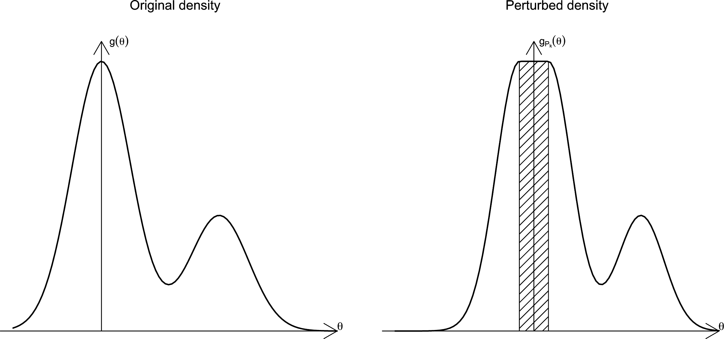
The inflated density ratio estimator is a different formulation of the GHM estimator, based on a particular choice of the instrumental density f (θ) as originally proposed in Petris and Tardella (2007). The instrumental f (θ) is obtained through a perturbation of the original target function g. The perturbed density, denoted with g_Pk, is defined so that its total mass has some known functional relation to the total mass c of the target density g as in equation (4). In particular, g_Pk is obtained as a parametric inflation of g so that \documentclass{aastex}\usepackage{amsbsy}\usepackage{amsfonts}\usepackage{amssymb}\usepackage{bm}\usepackage{mathrsfs}\usepackage{pifont}\usepackage{stmaryrd}\usepackage{textcomp}\usepackage{portland, xspace}\usepackage{amsmath, amsxtra}\pagestyle{empty}\DeclareMathSizes{10}{9}{7}{6}\begin{document} \begin{align*} \int_{\Omega}g_{P_{k}} (\theta) = c + k \tag{9} \end{align*} \end{document}

where k is a known inflation constant which can be arbitrarily fixed. The perturbation device comes from an original idea in Petris and Tardella (2003) and is detailed in Petris and Tardella (2007) for unidimensional and multidimensional densities. In the unidimensional case the perturbed density is \documentclass{aastex}\usepackage{amsbsy}\usepackage{amsfonts}\usepackage{amssymb}\usepackage{bm}\usepackage{mathrsfs}\usepackage{pifont}\usepackage{stmaryrd}\usepackage{textcomp}\usepackage{portland, xspace}\usepackage{amsmath, amsxtra}\pagestyle{empty}\DeclareMathSizes{10}{9}{7}{6}\begin{document} \begin{align*} g_{P_{k}} (\theta) = \begin{cases}g (\theta + r_{k}) \qquad \hbox{if} \ \theta < - r_{k} \\ g (0) \qquad \qquad \hbox{if} - r_{k} \leq \theta \leq r_{k} \\ g (\theta - r_{k}) \qquad \hbox{if} \ \theta > r_{k}\end{cases} \tag{10} \end{align*} \end{document}

with \documentclass{aastex}\usepackage{amsbsy}\usepackage{amsfonts}\usepackage{amssymb}\usepackage{bm}\usepackage{mathrsfs}\usepackage{pifont}\usepackage{stmaryrd}\usepackage{textcomp}\usepackage{portland, xspace}\usepackage{amsmath, amsxtra}\pagestyle{empty}\DeclareMathSizes{10}{9}{7}{6}\begin{document} $$2r_k = \frac {k} {g (0)}$$ \end{document} corresponding to the length of the interval centered around the origin where the density is kept constant. In Figure 1, one can visualize how the perturbation acts. The perturbed density allows one to define an instrumental density \documentclass{aastex}\usepackage{amsbsy}\usepackage{amsfonts}\usepackage{amssymb}\usepackage{bm}\usepackage{mathrsfs}\usepackage{pifont}\usepackage{stmaryrd}\usepackage{textcomp}\usepackage{portland, xspace}\usepackage{amsmath, amsxtra}\pagestyle{empty}\DeclareMathSizes{10}{9}{7}{6}\begin{document} $$f_{k} (\theta) = \frac {g_{P_{k}} (\theta) - g (\theta)} {k}$$ \end{document} which satisfies the requirement (6) needed to define the GHM estimator as in (7). The Inflated Density Ratio estimator \documentclass{aastex}\usepackage{amsbsy}\usepackage{amsfonts}\usepackage{amssymb}\usepackage{bm}\usepackage{mathrsfs}\usepackage{pifont}\usepackage{stmaryrd}\usepackage{textcomp}\usepackage{portland, xspace}\usepackage{amsmath, amsxtra}\pagestyle{empty}\DeclareMathSizes{10}{9}{7}{6}\begin{document} $$\hat{c}_{IDR}$$ \end{document} for c is then obtained as follows \documentclass{aastex}\usepackage{amsbsy}\usepackage{amsfonts}\usepackage{amssymb}\usepackage{bm}\usepackage{mathrsfs}\usepackage{pifont}\usepackage{stmaryrd}\usepackage{textcomp}\usepackage{portland, xspace}\usepackage{amsmath, amsxtra}\pagestyle{empty}\DeclareMathSizes{10}{9}{7}{6}\begin{document} \begin{align*} \hat {c}_{IDR} = \frac {k} {\frac {1} {T} \sum_{t = 1}^{T} \frac {g_{P_{k}} (\theta_{t})} {g (\theta_{t})} - 1} \tag {11} \end{align*} \end{document}

OPEN IN VIEWER

FIG. 1.

(Left) original density g with total mass c. (Right) perturbed density \documentclass{aastex}\usepackage{amsbsy}\usepackage{amsfonts}\usepackage{amssymb}\usepackage{bm}\usepackage{mathrsfs}\usepackage{pifont}\usepackage{stmaryrd}\usepackage{textcomp}\usepackage{portland, xspace}\usepackage{amsmath, amsxtra}\pagestyle{empty}\DeclareMathSizes{10}{9}{7}{6}\begin{document} $$g_{P_{k}}$$ \end{document} defined as in equation (10). The total mass of the perturbed density is then c + k. The shaded area correspond to the inflated mass k with k = 2 · r_k · g(0) as in (10).

where \documentclass{aastex}\usepackage{amsbsy}\usepackage{amsfonts}\usepackage{amssymb}\usepackage{bm}\usepackage{mathrsfs}\usepackage{pifont}\usepackage{stmaryrd}\usepackage{textcomp}\usepackage{portland, xspace}\usepackage{amsmath, amsxtra}\pagestyle{empty}\DeclareMathSizes{10}{9}{7}{6}\begin{document} $$\theta_{1}, \ldots, \theta_{T}$$ \end{document} is a sample from the normalized target density \documentclass{aastex}\usepackage{amsbsy}\usepackage{amsfonts}\usepackage{amssymb}\usepackage{bm}\usepackage{mathrsfs}\usepackage{pifont}\usepackage{stmaryrd}\usepackage{textcomp}\usepackage{portland, xspace}\usepackage{amsmath, amsxtra}\pagestyle{empty}\DeclareMathSizes{10}{9}{7}{6}\begin{document} $$\tilde{g}$$ \end{document} . The use of the perturbed density as importance function leads to some advantages with respect to the other instances of c_GHM proposed in the literature. In fact \documentclass{aastex}\usepackage{amsbsy}\usepackage{amsfonts}\usepackage{amssymb}\usepackage{bm}\usepackage{mathrsfs}\usepackage{pifont}\usepackage{stmaryrd}\usepackage{textcomp}\usepackage{portland, xspace}\usepackage{amsmath, amsxtra}\pagestyle{empty}\DeclareMathSizes{10}{9}{7}{6}\begin{document} $$\hat{c}_{IDR}$$ \end{document} yields a finite-variance estimator under mild sufficient conditions and a wide range of g densities (Petris and Tardella, 2007) (Lemma, 1, 2, and 3). Notice that in order for the perturbed density g_Pk to be defined it is required that the original density g has full support in \documentclass{aastex}\usepackage{amsbsy}\usepackage{amsfonts}\usepackage{amssymb}\usepackage{bm}\usepackage{mathrsfs}\usepackage{pifont}\usepackage{stmaryrd}\usepackage{textcomp}\usepackage{portland, xspace}\usepackage{amsmath, amsxtra}\pagestyle{empty}\DeclareMathSizes{10}{9}{7}{6}\begin{document} $$\Re^k$$ \end{document} . Moreover, the use of a parametric perturbation makes the method more flexible and efficient with a moderate extra computational effort.

Like all methods based on importance sampling strategies, the properties of the estimator \documentclass{aastex}\usepackage{amsbsy}\usepackage{amsfonts}\usepackage{amssymb}\usepackage{bm}\usepackage{mathrsfs}\usepackage{pifont}\usepackage{stmaryrd}\usepackage{textcomp}\usepackage{portland, xspace}\usepackage{amsmath, amsxtra}\pagestyle{empty}\DeclareMathSizes{10}{9}{7}{6}\begin{document} $$\hat{c}_{IDR}$$ \end{document} strongly depend on the ratio \documentclass{aastex}\usepackage{amsbsy}\usepackage{amsfonts}\usepackage{amssymb}\usepackage{bm}\usepackage{mathrsfs}\usepackage{pifont}\usepackage{stmaryrd}\usepackage{textcomp}\usepackage{portland, xspace}\usepackage{amsmath, amsxtra}\pagestyle{empty}\DeclareMathSizes{10}{9}{7}{6}\begin{document} $$\frac {g_{P_{k}} (\theta)} {g (\theta)}$$ \end{document} . To evaluate its performance one can use an asymptotic approximation (as t →+∞) via standard delta-method of the Relative Mean Square Error of the estimator \documentclass{aastex}\usepackage{amsbsy}\usepackage{amsfonts}\usepackage{amssymb}\usepackage{bm}\usepackage{mathrsfs}\usepackage{pifont}\usepackage{stmaryrd}\usepackage{textcomp}\usepackage{portland, xspace}\usepackage{amsmath, amsxtra}\pagestyle{empty}\DeclareMathSizes{10}{9}{7}{6}\begin{document} \begin{align*} RMSE_{\hat {c}_{IDR}} = \sqrt {E_{\tilde {g}} \Bigg[\left(\frac {\hat {c}_{IDR} - c} {c} \right)^{2} \Bigg]} \approx \frac {c} {k} \sqrt {Var \Bigg[\frac {g_{P_{k}} (\theta)} {g (\theta)} \Bigg]} = RMSE_{\hat {c}_{IDR, Delta}} \tag {12} \end{align*} \end{document}

which can be ultimately estimated as follows: \documentclass{aastex}\usepackage{amsbsy}\usepackage{amsfonts}\usepackage{amssymb}\usepackage{bm}\usepackage{mathrsfs}\usepackage{pifont}\usepackage{stmaryrd}\usepackage{textcomp}\usepackage{portland, xspace}\usepackage{amsmath, amsxtra}\pagestyle{empty}\DeclareMathSizes{10}{9}{7}{6}\begin{document} \begin{align*} {\widehat {RMSE}}_{\hat {c}_{IDR, Delta}} = \frac {\hat {c}_{IDR}} {k} \sqrt {\widehat {Var}_{\tilde {g}} \Bigg[\frac {g_{P_{k}} (\theta)} {g (\theta)} \Bigg]} \tag {13} \end{align*} \end{document}

where \documentclass{aastex}\usepackage{amsbsy}\usepackage{amsfonts}\usepackage{amssymb}\usepackage{bm}\usepackage{mathrsfs}\usepackage{pifont}\usepackage{stmaryrd}\usepackage{textcomp}\usepackage{portland, xspace}\usepackage{amsmath, amsxtra}\pagestyle{empty}\DeclareMathSizes{10}{9}{7}{6}\begin{document} $$\widehat{Var}_{\tilde{g}}$$ \end{document} is the observed sample variance of the ratio g_Pk(θ)/g(θ).

The expression in equation (13) clarifies the key role of the choice of k with respect to the error of the estimator: for k → 0, the variance of the ratio \documentclass{aastex}\usepackage{amsbsy}\usepackage{amsfonts}\usepackage{amssymb}\usepackage{bm}\usepackage{mathrsfs}\usepackage{pifont}\usepackage{stmaryrd}\usepackage{textcomp}\usepackage{portland, xspace}\usepackage{amsmath, amsxtra}\pagestyle{empty}\DeclareMathSizes{10}{9}{7}{6}\begin{document} $$\frac {g_{P_{k}} (\theta)} {g (\theta)}$$ \end{document} tends to 0, since g_Pk is very close to g, but \documentclass{aastex}\usepackage{amsbsy}\usepackage{amsfonts}\usepackage{amssymb}\usepackage{bm}\usepackage{mathrsfs}\usepackage{pifont}\usepackage{stmaryrd}\usepackage{textcomp}\usepackage{portland, xspace}\usepackage{amsmath, amsxtra}\pagestyle{empty}\DeclareMathSizes{10}{9}{7}{6}\begin{document} $$\frac {c} {k}$$ \end{document} tends to infinity: in other words, if \documentclass{aastex}\usepackage{amsbsy}\usepackage{amsfonts}\usepackage{amssymb}\usepackage{bm}\usepackage{mathrsfs}\usepackage{pifont}\usepackage{stmaryrd}\usepackage{textcomp}\usepackage{portland, xspace}\usepackage{amsmath, amsxtra}\pagestyle{empty}\DeclareMathSizes{10}{9}{7}{6}\begin{document} $$Var_{\tilde {g}} \left[\frac {g_{P_{k}} (\theta)} {g (\theta)} \right]$$ \end{document} would favor as little values of k as possible, \documentclass{aastex}\usepackage{amsbsy}\usepackage{amsfonts}\usepackage{amssymb}\usepackage{bm}\usepackage{mathrsfs}\usepackage{pifont}\usepackage{stmaryrd}\usepackage{textcomp}\usepackage{portland, xspace}\usepackage{amsmath, amsxtra}\pagestyle{empty}\DeclareMathSizes{10}{9}{7}{6}\begin{document} $$\frac {1} {k}$$ \end{document} acts in the opposite direction. In order to address the choice of k, Petris and Tardella (2007) suggested to choose the perturbation k which minimizes the estimation error (13). In practice, one can calculate the values of the estimator for a grid of different perturbation values, \documentclass{aastex}\usepackage{amsbsy}\usepackage{amsfonts}\usepackage{amssymb}\usepackage{bm}\usepackage{mathrsfs}\usepackage{pifont}\usepackage{stmaryrd}\usepackage{textcomp}\usepackage{portland, xspace}\usepackage{amsmath, amsxtra}\pagestyle{empty}\DeclareMathSizes{10}{9}{7}{6}\begin{document} $$\hat{c}_{IDR} (k), k = 1, \ldots, K$$ \end{document} and choose the optimal k^opt as the k for which \documentclass{aastex}\usepackage{amsbsy}\usepackage{amsfonts}\usepackage{amssymb}\usepackage{bm}\usepackage{mathrsfs}\usepackage{pifont}\usepackage{stmaryrd}\usepackage{textcomp}\usepackage{portland, xspace}\usepackage{amsmath, amsxtra}\pagestyle{empty}\DeclareMathSizes{10}{9}{7}{6}\begin{document} $${\widehat {RMSE}}_{\hat{c}_{IDR} (k)}$$ \end{document} is minimum. This procedure for the calibration of k requires iterative evaluation of \documentclass{aastex}\usepackage{amsbsy}\usepackage{amsfonts}\usepackage{amssymb}\usepackage{bm}\usepackage{mathrsfs}\usepackage{pifont}\usepackage{stmaryrd}\usepackage{textcomp}\usepackage{portland, xspace}\usepackage{amsmath, amsxtra}\pagestyle{empty}\DeclareMathSizes{10}{9}{7}{6}\begin{document} $$\hat{c}_{IDR} (k)$$ \end{document} hence is relatively heavier than the HM estimator, but it does not require extra simulations which in the phylogenetic context is often the main time-consuming part. Hence, the computational cost is alleviated by the fact that one uses the same sample from \documentclass{aastex}\usepackage{amsbsy}\usepackage{amsfonts}\usepackage{amssymb}\usepackage{bm}\usepackage{mathrsfs}\usepackage{pifont}\usepackage{stmaryrd}\usepackage{textcomp}\usepackage{portland, xspace}\usepackage{amsmath, amsxtra}\pagestyle{empty}\DeclareMathSizes{10}{9}{7}{6}\begin{document} $$\tilde{g}$$ \end{document} and the only quantity to be evaluated K times is the inflated density g_Pk. Once obtained the ratio of the perturbed and the original density, the computation of \documentclass{aastex}\usepackage{amsbsy}\usepackage{amsfonts}\usepackage{amssymb}\usepackage{bm}\usepackage{mathrsfs}\usepackage{pifont}\usepackage{stmaryrd}\usepackage{textcomp}\usepackage{portland, xspace}\usepackage{amsmath, amsxtra}\pagestyle{empty}\DeclareMathSizes{10}{9}{7}{6}\begin{document} $$\hat{c}_{IDR} (k)$$ \end{document} is straightforward.

For practical purposes, the computation of the inflated density when the support of g is the whole \documentclass{aastex}\usepackage{amsbsy}\usepackage{amsfonts}\usepackage{amssymb}\usepackage{bm}\usepackage{mathrsfs}\usepackage{pifont}\usepackage{stmaryrd}\usepackage{textcomp}\usepackage{portland, xspace}\usepackage{amsmath, amsxtra}\pagestyle{empty}\DeclareMathSizes{10}{9}{7}{6}\begin{document} $$\Re^k$$ \end{document} can be easily implemented in R using a function available at http://sites.google.com/site/idrharmonicmean/home. In Arima (2009) and Petris and Tardella (2007), it has been shown that in order to improve the precision of \documentclass{aastex}\usepackage{amsbsy}\usepackage{amsfonts}\usepackage{amssymb}\usepackage{bm}\usepackage{mathrsfs}\usepackage{pifont}\usepackage{stmaryrd}\usepackage{textcomp}\usepackage{portland, xspace}\usepackage{amsmath, amsxtra}\pagestyle{empty}\DeclareMathSizes{10}{9}{7}{6}\begin{document} $$\hat{c}_{IDR}$$ \end{document} it is recommended to standardize the simulated data \documentclass{aastex}\usepackage{amsbsy}\usepackage{amsfonts}\usepackage{amssymb}\usepackage{bm}\usepackage{mathrsfs}\usepackage{pifont}\usepackage{stmaryrd}\usepackage{textcomp}\usepackage{portland, xspace}\usepackage{amsmath, amsxtra}\pagestyle{empty}\DeclareMathSizes{10}{9}{7}{6}\begin{document} $$\theta_1, \ldots, \theta_T$$ \end{document} with respect to a (local) mode and the sample variance-covariance matrix so that the corresponding density has a local mode at the origin and approximately standard variance-covariance matrix. This is automatically implemented in the publicly available R code.

In order to assess its effectiveness, the IDR method has been applied to simulated data from differently shaped distributions for which the normalizing constant is known. As shown in Petris and Tardella (2007), and confirmed by the numerical examples in Section 6, the estimator produces fully convincing results with simulated data from several known distributions, even for a 100-dimensional multivariate Gaussian distribution. In terms of estimator precision, these results are comparable with those in Lartillot and Philippe (2006) obtained with the thermodynamic integration. In Arima (2009), simple antithetic variate tricks allow the IDR estimator to perform well even for those distributions with severe variations from the symmetric Gaussian case such as asymmetric and even some multimodal distributions. In the next sections, we extend the IDR method in order to use \documentclass{aastex}\usepackage{amsbsy}\usepackage{amsfonts}\usepackage{amssymb}\usepackage{bm}\usepackage{mathrsfs}\usepackage{pifont}\usepackage{stmaryrd}\usepackage{textcomp}\usepackage{portland, xspace}\usepackage{amsmath, amsxtra}\pagestyle{empty}\DeclareMathSizes{10}{9}{7}{6}\begin{document} $$\hat{c}_{IDR}$$ \end{document} in more complex settings such as phylogenetic models.

4.2. Implementing IDR for substitution models with fixed topology

We extend the IDR approach in order to compute the marginal likelihood of phylogenetic models. In this section, we show how to compute the marginal likelihood when it involves integration of substitution model parameters θ and the branch lengths ν_τ which are both defined in continuous subspaces. Indeed the approach can be used as a building block to integrate also over the tree topology τ.

For a fixed topology τ and a sequence alignment X, the parameters of a phylogenetic model M_τ are denoted as ω = (θ, ν_τ) ⊂ Ω _τ . The joint posterior distribution on ω is given by \documentclass{aastex}\usepackage{amsbsy}\usepackage{amsfonts}\usepackage{amssymb}\usepackage{bm}\usepackage{mathrsfs}\usepackage{pifont}\usepackage{stmaryrd}\usepackage{textcomp}\usepackage{portland, xspace}\usepackage{amsmath, amsxtra}\pagestyle{empty}\DeclareMathSizes{10}{9}{7}{6}\begin{document} \begin{align*} p (\theta, \nu_{\tau} \mid X, M_\tau) = \frac {p (X \mid \theta, \nu_{\tau}, M_\tau) \pi_{\Theta} (\theta) \pi_{{\cal V}} (\nu_{\tau})} {m (X \mid M_\tau)} \tag {14} \end{align*} \end{document}

where \documentclass{aastex}\usepackage{amsbsy}\usepackage{amsfonts}\usepackage{amssymb}\usepackage{bm}\usepackage{mathrsfs}\usepackage{pifont}\usepackage{stmaryrd}\usepackage{textcomp}\usepackage{portland, xspace}\usepackage{amsmath, amsxtra}\pagestyle{empty}\DeclareMathSizes{10}{9}{7}{6}\begin{document} \begin{align*} m (X \mid M_{\tau}) = \int_{\theta} \int_{\nu_{\tau}}p (X \mid \theta, \nu_{\tau}, M_\tau) \pi_{\Theta} (\theta) \pi_{{\cal V}} (\nu_{\tau}) d \theta d \nu_{\tau} \tag{15} \end{align*} \end{document}

is the marginal likelihood we aim at estimating.

When the topology τ is fixed, the parameter space Ω_τ is continuous. Hence, in order to apply the IDR method we only need the following two ingredients:

• a sample \documentclass{aastex}\usepackage{amsbsy}\usepackage{amsfonts}\usepackage{amssymb}\usepackage{bm}\usepackage{mathrsfs}\usepackage{pifont}\usepackage{stmaryrd}\usepackage{textcomp}\usepackage{portland, xspace}\usepackage{amsmath, amsxtra}\pagestyle{empty}\DeclareMathSizes{10}{9}{7}{6}\begin{document} $$(\theta^{(1)}, \nu_{\tau}^{(1)}), \ldots, (\theta^{(T)}, \nu_{\tau}^{(T)})$$ \end{document} from the posterior distribution, p(θ, ν_τ|X, M_τ)

The first ingredient is just the usual output of the MCMC simulations derived from model M and data X. The computation of the likelihood and the joint prior is usually already coded within available software. The first one is accomplished through the pruning algorithm while computing the prior is straightforward. Indeed a necessary condition for the inflation idea to be implemented as prescribed in Petris and Tardella (2007) is that the posterior density must have full support on the whole real k-dimensional space. In our phylogenetic models, this is not always the case hence we explain simple and fully automatic remedies to overcome this kind of obstacle.

We start with branch length parameters which are constrained to lie in the positive half-line. In that case, the remedy is straightforward. One can reparameterize with a simple logarithmic transformation \documentclass{aastex}\usepackage{amsbsy}\usepackage{amsfonts}\usepackage{amssymb}\usepackage{bm}\usepackage{mathrsfs}\usepackage{pifont}\usepackage{stmaryrd}\usepackage{textcomp}\usepackage{portland, xspace}\usepackage{amsmath, amsxtra}\pagestyle{empty}\DeclareMathSizes{10}{9}{7}{6}\begin{document} \begin{align*} \nu^{\prime}_{\tau} = \log (\nu_{\tau}) \tag{16} \end{align*} \end{document}

so that the support corresponding to the reparameterized density becomes unconstrained. Obviously the log(ν_τ) reparameterization calls for the appropriate Jacobian when evaluating the corresponding transformed density. For model parameters with linear constraints like the substitution θ = {ρ, π}, a little less obvious transformation is needed. In this case, θ = {ρ, π} are subject to the following set of constraints: \documentclass{aastex}\usepackage{amsbsy}\usepackage{amsfonts}\usepackage{amssymb}\usepackage{bm}\usepackage{mathrsfs}\usepackage{pifont}\usepackage{stmaryrd}\usepackage{textcomp}\usepackage{portland, xspace}\usepackage{amsmath, amsxtra}\pagestyle{empty}\DeclareMathSizes{10}{9}{7}{6}\begin{document} \begin{align*} \sum_{i \in \{A, T, C, G \}} \pi_{i} & = 1 \\ \sum_{j \in \{A, T, C, G \}} \rho_{ij} \pi_{j} & = 0 \qquad \qquad \forall \ i \in \{A, T, C, G \} \end{align*} \end{document}

Similarly to the first simplex constraint the last set of constraints together with the reversibility can be rephrased (Gowri-Shankar, 2006) in terms of another simplex constraint concerning only the extra-diagonal entries of the substitution rate matrix (2) namely \documentclass{aastex}\usepackage{amsbsy}\usepackage{amsfonts}\usepackage{amssymb}\usepackage{bm}\usepackage{mathrsfs}\usepackage{pifont}\usepackage{stmaryrd}\usepackage{textcomp}\usepackage{portland, xspace}\usepackage{amsmath, amsxtra}\pagestyle{empty}\DeclareMathSizes{10}{9}{7}{6}\begin{document} \begin{align*} \rho_{AC} + \rho_{AG} + \rho_{AT} + \rho_{CG} + \rho_{CT} + \rho_{GT} = 1. \end{align*} \end{document}

In order to bypass the constrained nature of the parameter space we have relied on the so-called additive logistic transformation (Aitichinson, 1986; Tiao and Cuttman, 1965), which is a one-to-one transformation from \documentclass{aastex}\usepackage{amsbsy}\usepackage{amsfonts}\usepackage{amssymb}\usepackage{bm}\usepackage{mathrsfs}\usepackage{pifont}\usepackage{stmaryrd}\usepackage{textcomp}\usepackage{portland, xspace}\usepackage{amsmath, amsxtra}\pagestyle{empty}\DeclareMathSizes{10}{9}{7}{6}\begin{document} $${\mathbb R}^{D - 1}$$ \end{document} to the (D − 1)-dimensional simplex \documentclass{aastex}\usepackage{amsbsy}\usepackage{amsfonts}\usepackage{amssymb}\usepackage{bm}\usepackage{mathrsfs}\usepackage{pifont}\usepackage{stmaryrd}\usepackage{textcomp}\usepackage{portland, xspace}\usepackage{amsmath, amsxtra}\pagestyle{empty}\DeclareMathSizes{10}{9}{7}{6}\begin{document} \begin{align*} S^{D} = \left\{(x_{1}, \ldots, x_{D}) : x_{1} > 0, \ldots, x_{D} > 0; x_{1} + \ldots x_{D} = 1 \right\} . \end{align*} \end{document}

Hence, we can use its inverse, called additive log-ratio transformation, which is defined as follows \documentclass{aastex}\usepackage{amsbsy}\usepackage{amsfonts}\usepackage{amssymb}\usepackage{bm}\usepackage{mathrsfs}\usepackage{pifont}\usepackage{stmaryrd}\usepackage{textcomp}\usepackage{portland, xspace}\usepackage{amsmath, amsxtra}\pagestyle{empty}\DeclareMathSizes{10}{9}{7}{6}\begin{document} \begin{align*} y_{i} = \log \left(\frac {x_{i}} {x_{D}} \right) \qquad i = 1, \ldots, D - 1 \end{align*} \end{document}

for any \documentclass{aastex}\usepackage{amsbsy}\usepackage{amsfonts}\usepackage{amssymb}\usepackage{bm}\usepackage{mathrsfs}\usepackage{pifont}\usepackage{stmaryrd}\usepackage{textcomp}\usepackage{portland, xspace}\usepackage{amsmath, amsxtra}\pagestyle{empty}\DeclareMathSizes{10}{9}{7}{6}\begin{document} $$x = (x_1, \ldots, x_D) \in S^D$$ \end{document} . Here, the x _i 's are the ρ's and D = 6. Applying these transformations to nucleotide frequencies π_i and to exchangeability parameters ρ's, the transformed parameters assume values in the entire real support and the IDR estimator can be applied. Again, the reparameterization calls for the appropriate change-of-measure Jacobian when evaluating the corresponding transformed density (Aitichinson, 1986).

5.1. Generalized Stepping Stone (GSS) estimator

The GSS method, presented in Fan et al. (2011) is a modification of the SS method introduced in Xie et al. (2011). This method is closely related to the thermodynamic integration and shares with it the need of sampling from a discretized grid of intermediate distributions in addition to the posterior.

Using the same notation of the previous section, the GSS estimator is defined as \documentclass{aastex}\usepackage{amsbsy}\usepackage{amsfonts}\usepackage{amssymb}\usepackage{bm}\usepackage{mathrsfs}\usepackage{pifont}\usepackage{stmaryrd}\usepackage{textcomp}\usepackage{portland, xspace}\usepackage{amsmath, amsxtra}\pagestyle{empty}\DeclareMathSizes{10}{9}{7}{6}\begin{document} \begin{align*} c_{GSS} = \prod_{t = 1}^{T} \frac {c (\beta_{t})} {c (\beta_{t - 1})} \tag {21} \end{align*} \end{document}

where \documentclass{aastex}\usepackage{amsbsy}\usepackage{amsfonts}\usepackage{amssymb}\usepackage{bm}\usepackage{mathrsfs}\usepackage{pifont}\usepackage{stmaryrd}\usepackage{textcomp}\usepackage{portland, xspace}\usepackage{amsmath, amsxtra}\pagestyle{empty}\DeclareMathSizes{10}{9}{7}{6}\begin{document} \begin{align*} r_{t} = \frac {c (\beta_{t})} {c (\beta_{t - 1})} = E_{\tilde {q} (; \beta_{t - 1})} \left[\left(\frac {g (\theta)} {f (\theta)} \right)^{\beta_{t} - \beta_{t - 1}} \right] \tag {22} \end{align*} \end{document}

and \documentclass{aastex}\usepackage{amsbsy}\usepackage{amsfonts}\usepackage{amssymb}\usepackage{bm}\usepackage{mathrsfs}\usepackage{pifont}\usepackage{stmaryrd}\usepackage{textcomp}\usepackage{portland, xspace}\usepackage{amsmath, amsxtra}\pagestyle{empty}\DeclareMathSizes{10}{9}{7}{6}\begin{document} $$\tilde {q} (; \beta_{t}) = \frac {q (; \beta_{t})} {c (\beta_{t})} = \frac {g (\theta)^{\beta_{t}} f (\theta)^{1 - \beta_{t}}} {c (\beta_{t})}$$ \end{document} . In Fan et al. (2011), g(θ) is taken as the product of likelihood and prior and f (θ) is a reference distribution (π₀(θ)), which yields \documentclass{aastex}\usepackage{amsbsy}\usepackage{amsfonts}\usepackage{amssymb}\usepackage{bm}\usepackage{mathrsfs}\usepackage{pifont}\usepackage{stmaryrd}\usepackage{textcomp}\usepackage{portland, xspace}\usepackage{amsmath, amsxtra}\pagestyle{empty}\DeclareMathSizes{10}{9}{7}{6}\begin{document} \begin{align*} r_{t} = E_{\tilde {q} (; \beta_{t - 1})} \left[\left(\frac {L (\theta) \pi (\theta)} {\pi_{0} (\theta)} \right)^{\beta_{t} - \beta_{t - 1}} \right] \tag {23} \end{align*} \end{document}

where \documentclass{aastex}\usepackage{amsbsy}\usepackage{amsfonts}\usepackage{amssymb}\usepackage{bm}\usepackage{mathrsfs}\usepackage{pifont}\usepackage{stmaryrd}\usepackage{textcomp}\usepackage{portland, xspace}\usepackage{amsmath, amsxtra}\pagestyle{empty}\DeclareMathSizes{10}{9}{7}{6}\begin{document} $$\tilde {q} (; \beta_{t}) = \frac {(L (\theta) \pi (\theta))^{\beta_{t}} \pi_{0} (\theta)^{1 - \beta_{t}}} {c (\beta_{t})}$$ \end{document} . The density \documentclass{aastex}\usepackage{amsbsy}\usepackage{amsfonts}\usepackage{amssymb}\usepackage{bm}\usepackage{mathrsfs}\usepackage{pifont}\usepackage{stmaryrd}\usepackage{textcomp}\usepackage{portland, xspace}\usepackage{amsmath, amsxtra}\pagestyle{empty}\DeclareMathSizes{10}{9}{7}{6}\begin{document} $$\tilde{q} (; \beta_t)$$ \end{document} is equivalent to the posterior distribution when β = 1 and it is equivalent to the reference distribution when β = 0. The expression in (23) can be estimated using \documentclass{aastex}\usepackage{amsbsy}\usepackage{amsfonts}\usepackage{amssymb}\usepackage{bm}\usepackage{mathrsfs}\usepackage{pifont}\usepackage{stmaryrd}\usepackage{textcomp}\usepackage{portland, xspace}\usepackage{amsmath, amsxtra}\pagestyle{empty}\DeclareMathSizes{10}{9}{7}{6}\begin{document} \begin{align*} \hat {r}_{t} = \frac {1} {n} \sum_{i = 1}^{n} \left(\frac {L (\theta_{i, \beta_{t - 1}}) \pi (\theta_{i, \beta_{t - 1}})} {\pi_{0} (\theta_{i, \beta_{t - 1}})} \right) \end{align*} \end{document}

where \documentclass{aastex}\usepackage{amsbsy}\usepackage{amsfonts}\usepackage{amssymb}\usepackage{bm}\usepackage{mathrsfs}\usepackage{pifont}\usepackage{stmaryrd}\usepackage{textcomp}\usepackage{portland, xspace}\usepackage{amsmath, amsxtra}\pagestyle{empty}\DeclareMathSizes{10}{9}{7}{6}\begin{document} $$\theta_{1, \beta_{t}}, \theta_{2, \beta_{t}}, \ldots, \theta_{n, \beta_{t}} \sim \tilde{q} (\theta; \beta_{t})$$ \end{document} . Hence, the GSS estimator is defined as \documentclass{aastex}\usepackage{amsbsy}\usepackage{amsfonts}\usepackage{amssymb}\usepackage{bm}\usepackage{mathrsfs}\usepackage{pifont}\usepackage{stmaryrd}\usepackage{textcomp}\usepackage{portland, xspace}\usepackage{amsmath, amsxtra}\pagestyle{empty}\DeclareMathSizes{10}{9}{7}{6}\begin{document} \begin{align*} \widehat{c}_{GSS} = \prod_{t = 1}^{T} \hat{r}_{t} \end{align*} \end{document}

In Fan et al. (2011), the reference distribution π₀(·) is constructed using the same parameterized functional form of the prior distribution and calibrated using samples from the posterior distribution \documentclass{aastex}\usepackage{amsbsy}\usepackage{amsfonts}\usepackage{amssymb}\usepackage{bm}\usepackage{mathrsfs}\usepackage{pifont}\usepackage{stmaryrd}\usepackage{textcomp}\usepackage{portland, xspace}\usepackage{amsmath, amsxtra}\pagestyle{empty}\DeclareMathSizes{10}{9}{7}{6}\begin{document} $$\tilde{q} (\cdot ; \beta = 1)$$ \end{document} : parameters of the reference distribution are set equal to the posterior mean of the same parameters drawn from \documentclass{aastex}\usepackage{amsbsy}\usepackage{amsfonts}\usepackage{amssymb}\usepackage{bm}\usepackage{mathrsfs}\usepackage{pifont}\usepackage{stmaryrd}\usepackage{textcomp}\usepackage{portland, xspace}\usepackage{amsmath, amsxtra}\pagestyle{empty}\DeclareMathSizes{10}{9}{7}{6}\begin{document} $$\tilde{q} (\cdot ; \beta = 1)$$ \end{document} . The relative mean square error of \documentclass{aastex}\usepackage{amsbsy}\usepackage{amsfonts}\usepackage{amssymb}\usepackage{bm}\usepackage{mathrsfs}\usepackage{pifont}\usepackage{stmaryrd}\usepackage{textcomp}\usepackage{portland, xspace}\usepackage{amsmath, amsxtra}\pagestyle{empty}\DeclareMathSizes{10}{9}{7}{6}\begin{document} $$\hat{c}_{GSS}$$ \end{document} can be approximated as follows \documentclass{aastex}\usepackage{amsbsy}\usepackage{amsfonts}\usepackage{amssymb}\usepackage{bm}\usepackage{mathrsfs}\usepackage{pifont}\usepackage{stmaryrd}\usepackage{textcomp}\usepackage{portland, xspace}\usepackage{amsmath, amsxtra}\pagestyle{empty}\DeclareMathSizes{10}{9}{7}{6}\begin{document} \begin{align*} {\widehat {RMSE}}_{\hat {c}_{GSS}} \approx \frac {1} {n^{2}} \sum_{t = 1}^{T} \sum_{i = 1}^{n} \left(\frac {\widehat {c}_{GSS, i, t}} {\widehat {c}_{GSS, t}} - 1 \right)^{2} \tag {24} \end{align*} \end{document}

The GSS reduces to the original SS method proposed in Xie et al. (2011) if the reference distribution is equal to the actual prior: \documentclass{aastex}\usepackage{amsbsy}\usepackage{amsfonts}\usepackage{amssymb}\usepackage{bm}\usepackage{mathrsfs}\usepackage{pifont}\usepackage{stmaryrd}\usepackage{textcomp}\usepackage{portland, xspace}\usepackage{amsmath, amsxtra}\pagestyle{empty}\DeclareMathSizes{10}{9}{7}{6}\begin{document} \begin{align*} \hat {r}_{t}^{SS} = \frac {1} {n} \sum_{i = 1}^{n} L (\theta_{i, \beta_{t - 1}}) \tag {25} \end{align*} \end{document}

where \documentclass{aastex}\usepackage{amsbsy}\usepackage{amsfonts}\usepackage{amssymb}\usepackage{bm}\usepackage{mathrsfs}\usepackage{pifont}\usepackage{stmaryrd}\usepackage{textcomp}\usepackage{portland, xspace}\usepackage{amsmath, amsxtra}\pagestyle{empty}\DeclareMathSizes{10}{9}{7}{6}\begin{document} $$\theta_{i, \beta_{t}} \sim \tilde {q} (; \beta_{t}) = \frac {L (\theta)^{\beta_{t}} \pi (\theta)} {c (\beta_{t})}$$ \end{document} , and the SS estimator is defined as \documentclass{aastex}\usepackage{amsbsy}\usepackage{amsfonts}\usepackage{amssymb}\usepackage{bm}\usepackage{mathrsfs}\usepackage{pifont}\usepackage{stmaryrd}\usepackage{textcomp}\usepackage{portland, xspace}\usepackage{amsmath, amsxtra}\pagestyle{empty}\DeclareMathSizes{10}{9}{7}{6}\begin{document} \begin{align*} \hat{c}_{SS} = \prod_{t = 1}^{T} \hat{r}_{t}^{SS} \tag{26} \end{align*} \end{document}

In Fan et al. (2011), it is argued that GSS is more reliable and efficient than the other methods, such as the harmonic mean, the stepping stone method and the path sampling estimator.

7.1. Hadamard data: marginal likelihood computation

We use as a first benchmark the synthetic data set Hadamard already employed in Felsenstein (2004). It consists of 200 amino acids and four species (A, B, C, and D). This dataset have been simulated from the Jukes-Cantor model (JC69), and the true tree is shown in the left panel of Figure 2.

OPEN IN VIEWER

FIG. 2.

True phylogenetic trees of the two data sets used as benchmarks: Hadamard (left) and Green (right).

For the true topology, we compute the marginal likelihood for the JC69 model and for the GTR + Γ model: parameters lie in a five-dimensional space for the JC69 model and in 14-dimensional space for the GTR + Γ model. The simulated values from the Metropolis-Coupled algorithm have been rearranged to evaluate the model evidence of both models using different variants of the GHM and thermodynamic integration approaches.

GTR + Γ and JC69 models have been implemented in Phycas which provides as output the simulated Markov chains. Simulated values from \documentclass{aastex}\usepackage{amsbsy}\usepackage{amsfonts}\usepackage{amssymb}\usepackage{bm}\usepackage{mathrsfs}\usepackage{pifont}\usepackage{stmaryrd}\usepackage{textcomp}\usepackage{portland, xspace}\usepackage{amsmath, amsxtra}\pagestyle{empty}\DeclareMathSizes{10}{9}{7}{6}\begin{document} $$\tilde{q} (\cdot, \beta_t = 1)$$ \end{document} can be used as a sample from the posterior distribution in order to make inference on the model parameters.

In Table 3, we list the corresponding values of the IDR estimator on the log scale ( \documentclass{aastex}\usepackage{amsbsy}\usepackage{amsfonts}\usepackage{amssymb}\usepackage{bm}\usepackage{mathrsfs}\usepackage{pifont}\usepackage{stmaryrd}\usepackage{textcomp}\usepackage{portland, xspace}\usepackage{amsmath, amsxtra}\pagestyle{empty}\DeclareMathSizes{10}{9}{7}{6}\begin{document} $$\log \hat{c}_{IDR}$$ \end{document} ), the Relative Mean Square Error (RMSE) estimate ( \documentclass{aastex}\usepackage{amsbsy}\usepackage{amsfonts}\usepackage{amssymb}\usepackage{bm}\usepackage{mathrsfs}\usepackage{pifont}\usepackage{stmaryrd}\usepackage{textcomp}\usepackage{portland, xspace}\usepackage{amsmath, amsxtra}\pagestyle{empty}\DeclareMathSizes{10}{9}{7}{6}\begin{document} $${\widehat {RMSE}}_{\hat{c}_{IDR}}$$ \end{document} ) as in equation (13) and the confidence interval \documentclass{aastex}\usepackage{amsbsy}\usepackage{amsfonts}\usepackage{amssymb}\usepackage{bm}\usepackage{mathrsfs}\usepackage{pifont}\usepackage{stmaryrd}\usepackage{textcomp}\usepackage{portland, xspace}\usepackage{amsmath, amsxtra}\pagestyle{empty}\DeclareMathSizes{10}{9}{7}{6}\begin{document} $$\widehat{CI}$$ \end{document} for different perturbation masses k. In order to take into account the autocorrelation of the posterior simulated values, a correction has been applied to \documentclass{aastex}\usepackage{amsbsy}\usepackage{amsfonts}\usepackage{amssymb}\usepackage{bm}\usepackage{mathrsfs}\usepackage{pifont}\usepackage{stmaryrd}\usepackage{textcomp}\usepackage{portland, xspace}\usepackage{amsmath, amsxtra}\pagestyle{empty}\DeclareMathSizes{10}{9}{7}{6}\begin{document} $${\widehat {RMSE}}_{\hat{c}_{IDR}}$$ \end{document} replacing n in (13) with the effective sample size given by \documentclass{aastex}\usepackage{amsbsy}\usepackage{amsfonts}\usepackage{amssymb}\usepackage{bm}\usepackage{mathrsfs}\usepackage{pifont}\usepackage{stmaryrd}\usepackage{textcomp}\usepackage{portland, xspace}\usepackage{amsmath, amsxtra}\pagestyle{empty}\DeclareMathSizes{10}{9}{7}{6}\begin{document} \begin{align*} {n}_{ESS} = n \times \frac {1} {1 + 2 \sum_{i = 1}^{I} \hat {\rho}_i} \tag {27} \end{align*} \end{document}

with I = 10. Since the optimal corrected error \documentclass{aastex}\usepackage{amsbsy}\usepackage{amsfonts}\usepackage{amssymb}\usepackage{bm}\usepackage{mathrsfs}\usepackage{pifont}\usepackage{stmaryrd}\usepackage{textcomp}\usepackage{portland, xspace}\usepackage{amsmath, amsxtra}\pagestyle{empty}\DeclareMathSizes{10}{9}{7}{6}\begin{document} $$\widehat{CI}$$ \end{document} corresponds to a perturbation value k^opt = 10⁻⁶, the IDR estimator (on a logarithmic scale) for the JC model is log \documentclass{aastex}\usepackage{amsbsy}\usepackage{amsfonts}\usepackage{amssymb}\usepackage{bm}\usepackage{mathrsfs}\usepackage{pifont}\usepackage{stmaryrd}\usepackage{textcomp}\usepackage{portland, xspace}\usepackage{amsmath, amsxtra}\pagestyle{empty}\DeclareMathSizes{10}{9}{7}{6}\begin{document} $$\log \hat{c}_{IDR} = - 592.2874$$ \end{document} .

For comparative purposes, we considered the results of the IDR method with those obtained with the original HM and GHM based on the same reference distribution π₀ which is used to implement the GSS as in Fan et al. (2011). Indeed to verify the impact of the choice of the initial distribution we also evaluate the estimates resulting from GSS and SS. The path sampling estimator and its generalized version have been also computed. The evaluation of all these thermodynamic alternatives were simple to implement since the reference distribution as well as the prior together with their evaluation on the sampled parameters are available from the Phycas output.

RMSEs of the HM estimators have been computed adapting the formula (13) while RMSEs of the thermodynamic estimators have been computed adapting the formula (24). For the adjusted RMSEs the effective sample size in (27) has been used. For each method, the Monte Carlo relative error of the estimate has been computed re-estimating the model 10 times ( \documentclass{aastex}\usepackage{amsbsy}\usepackage{amsfonts}\usepackage{amssymb}\usepackage{bm}\usepackage{mathrsfs}\usepackage{pifont}\usepackage{stmaryrd}\usepackage{textcomp}\usepackage{portland, xspace}\usepackage{amsmath, amsxtra}\pagestyle{empty}\DeclareMathSizes{10}{9}{7}{6}\begin{document} $$\widehat{RMSE}_{\hat{c}, MC}$$ \end{document} ) and recording the corresponding different values of \documentclass{aastex}\usepackage{amsbsy}\usepackage{amsfonts}\usepackage{amssymb}\usepackage{bm}\usepackage{mathrsfs}\usepackage{pifont}\usepackage{stmaryrd}\usepackage{textcomp}\usepackage{portland, xspace}\usepackage{amsmath, amsxtra}\pagestyle{empty}\DeclareMathSizes{10}{9}{7}{6}\begin{document} $$\hat{c}$$ \end{document} . Although it is known that under critical conditions such MC error is not sufficient to guarantee its precision it still remains a necessary premise for an accurate estimate.

The methods produce different results which were overall closer in the JC model while sometimes very distant in the GTR + Γ case. The closest marginal likelihood estimates are those from GSS, GPS, and GHM, all methods relying on the same reference distribution. Also SS estimates are quite close to those obtained with GSS. IDR and PS produce estimates which are very similar in both models although only slightly different from the previous ones. On the other hand, HM estimates can be very far apart. This is particularly evident in the GTR + Γ case, confirming that HM can be badly biased and unstable resulting in a seriously doubtful reliability. In the JC model, all methods, with the exception of HM, produce similar results: the corresponding estimates of the relative error, once adjusted for the autocorrelation, show that GPS and GSS are the most stable methods followed by IDR and PS. On the other hand, for the GTR + Γ model all estimates, with the exception of HM, are comparable although IDR results in the largest estimated error. This is also confirmed by the Monte Carlo error. Indeed we notice that the Monte Carlo estimates of the relative error do not always reflect well the theoretical estimates even when not accounting the autocorrelation. This could be explained by the presence of some bias in the corresponding estimates possibly due to choice of a not sufficiently dense grid or a not appropriate starting density such as the prior in the path sampling. This is particularly evident always for HM and for GHM and SS especially in the GRT + Γ model. For GSS, GPS, PS, and IDR, the Monte Carlo errors always fall in between the one estimated as with an independent sample and the one accounting for the presence of autocorrelation.

In order to better visualize the results in Table 4, Figure 3 shows the marginal likelihoods (on logarithmic scale) for JC69 and GTR + Γ model. Considering the reference values for the Bayes Factor defined in Kass and Raftery (1995), all methods, with the exception of HM, strongly and consistently give support to the Jukes-Cantor model, which is known in this case to be the true model. We also point out that the estimates BF are all very similar.

OPEN IN VIEWER

FIG. 3.

Hadamard data: Log marginal likelihood estimated with HM, GHM, IDR, GSS, and SS methods for JC and GTR + Γ models. The estimated values are reported in Table 4.

7.2. Hadamard data: tree selection

We now show how it is possible to extend the IDR approach for dealing with selecting competing trees when the topology is not fixed in advance. For a fixed substitution model, competing trees can be compared by considering the evidence of the data for a fixed tree topology. The evidence in support of each tree topology \documentclass{aastex}\usepackage{amsbsy}\usepackage{amsfonts}\usepackage{amssymb}\usepackage{bm}\usepackage{mathrsfs}\usepackage{pifont}\usepackage{stmaryrd}\usepackage{textcomp}\usepackage{portland, xspace}\usepackage{amsmath, amsxtra}\pagestyle{empty}\DeclareMathSizes{10}{9}{7}{6}\begin{document} $$\tau_i \in N_T$$ \end{document} can be evaluated in terms of its posterior probability p(τ_i|X) derived from the Bayes theorem as \documentclass{aastex}\usepackage{amsbsy}\usepackage{amsfonts}\usepackage{amssymb}\usepackage{bm}\usepackage{mathrsfs}\usepackage{pifont}\usepackage{stmaryrd}\usepackage{textcomp}\usepackage{portland, xspace}\usepackage{amsmath, amsxtra}\pagestyle{empty}\DeclareMathSizes{10}{9}{7}{6}\begin{document} \begin{align*} p (\tau_{i} \mid X) = \frac {p (X \mid \tau_{i}) \pi_{{\cal T}} (\tau_{i})} {\sum_{\tau \in N_T} p (X \mid \tau) \pi_{{\cal T}} (\tau)} \end{align*} \end{document}

where the experimental evidence in favor of the model M_τi with fixed tree topology τ_i is contained in the marginal likelihood \documentclass{aastex}\usepackage{amsbsy}\usepackage{amsfonts}\usepackage{amssymb}\usepackage{bm}\usepackage{mathrsfs}\usepackage{pifont}\usepackage{stmaryrd}\usepackage{textcomp}\usepackage{portland, xspace}\usepackage{amsmath, amsxtra}\pagestyle{empty}\DeclareMathSizes{10}{9}{7}{6}\begin{document} \begin{align*} m (X \mid M_{\tau_{i}}) = p (X \mid \tau_{i}) = \int_{\Omega_{\tau_i}} p (X \mid \omega_i, M_{\tau_{i}}) \pi (\omega_i \mid \tau_{i}) d \omega_i \end{align*} \end{document}

where the continuous parameters \documentclass{aastex}\usepackage{amsbsy}\usepackage{amsfonts}\usepackage{amssymb}\usepackage{bm}\usepackage{mathrsfs}\usepackage{pifont}\usepackage{stmaryrd}\usepackage{textcomp}\usepackage{portland, xspace}\usepackage{amsmath, amsxtra}\pagestyle{empty}\DeclareMathSizes{10}{9}{7}{6}\begin{document} $$\omega_i \in \Omega_{\tau i}$$ \end{document} of the evolutionary process corresponding to Mτ_i are integrated out as nuisance parameters. Indeed, when prior beliefs on trees are set equal π(τ_i) = π(τ_j) comparative evidence discriminating τ_i against τ_j, is summarized in the BF \documentclass{aastex}\usepackage{amsbsy}\usepackage{amsfonts}\usepackage{amssymb}\usepackage{bm}\usepackage{mathrsfs}\usepackage{pifont}\usepackage{stmaryrd}\usepackage{textcomp}\usepackage{portland, xspace}\usepackage{amsmath, amsxtra}\pagestyle{empty}\DeclareMathSizes{10}{9}{7}{6}\begin{document} \begin{align*} BF_{ij} = \frac {m (X \mid M_{\tau_{i}})} {m (X \mid M_{\tau_{j}})}. \tag {28} \end{align*} \end{document}

We have considered the problem of selecting competing trees of a substitution model for Hadamard data. In the previous subsection, we have verified the feasibility and effectiveness of the IDR approach in comparing JC69 with the GTR + Γ model. Under a fixed topology, JC69 was favored. Indeed, we know that Hadamard data was simulated from the JC69 model with true topology labeled as τ = 1. Hence, we can compare N_T = 3 alternative topologies within the JC69 model computing the corresponding estimates of the marginal likelihoods and finally evaluate tree selection in terms of the pairwise BF. Results are shown in Table 5.

In this case, all methods allow to correctly favor the true topology with an estimate of the BF in favor of τ = 1, which ranges from strong to decisive. However, the original HM estimate is affected by a very large variability so that the confidence interval of the corresponding BF cannot lead to a clear conclusion. On the other hand, although the other methods are similarly conclusive, even accounting for estimate variability, the IDR method yields the most supporting evidence in favor of the true tree.

7.3. Green Plant rbcL example

We analyze the same green plant data used in Xie et al. (2011) (Table 6). Green plant data consists of 10 taxons and DNA sequences of the chloroplast-encoded large subunit of the RuBisCO gene (rbcL) (1296 amino acids). Following Xie et al. (2011) we use the topology shown in the right panel of Figure 1.

Again, we fit JC69 and GTR + Γ models and compare HM, GHM, IDR, SS, GSS, GPS, and PS marginal likelihood estimates. Original HM method appears to be unstable and remarkably different from all the other methods. GHM, GSS, and GPS give the most similar estimates. On the other hand, IDR, although showing larger error estimates, agrees with all the other methods and is very similar to PS.

Similar arguments apply when the GTR + Γ model is considered: all methods, with the exception of HM, produce very close estimates and, when accounted for the autocorrelation, also error estimates are comparable. However, SS method produces different results when applied to GTR + Γ model according to different choices of grid points: it appears that the auxiliary distribution whose quantiles are used to set the β grid plays here a key role in better estimating the marginal likelihood.

As far as model comparison is concerned the GTR + Γ model is strongly supported by all methods. Also in this case, HM reveals itself unreliable and not conclusive because of the larger error. On the other hand, the other methods give similar results. Despite some difference of the estimates produced by IDR, those differences are mitigated when BF is considered with IDR providing a slightly stronger evidence in favor of GTR + Gamma model.

In these examples, GSS and GPS are the most stable methods with respect to estimation error, and are somewhat robust with respect to the specification of the auxiliary distribution used to set the grid of β values. The stability of the results is possibly due to the fact that the reference distribution π₀ is well calibrated and closely resembles the posterior distribution. In Table 7, we investigate the robustness of the GSS estimates with respect to change of scale of the reference distribution. In particular, for the branch length parameters ν_τ the reference distribution is specified as the product of independent and identically distributed gamma distributions with shape α₁ and rate α₂ which are estimated using simulations from the posterior distribution. We modify the scale of the reference distribution considering as reference a gamma distribution with shape \documentclass{aastex}\usepackage{amsbsy}\usepackage{amsfonts}\usepackage{amssymb}\usepackage{bm}\usepackage{mathrsfs}\usepackage{pifont}\usepackage{stmaryrd}\usepackage{textcomp}\usepackage{portland, xspace}\usepackage{amsmath, amsxtra}\pagestyle{empty}\DeclareMathSizes{10}{9}{7}{6}\begin{document} $$\frac {\alpha_1} {\lambda}$$ \end{document} and rate α₂λ where λ is the perturbation factor. The same is done for the reference distribution component of the Γ parameter. For the substitution rates, we perturbed the original reference distribution multiplying all Dirichlet parameters for λ. Table 7 shows GSS can be affected by some variation in the scale of the reference distribution.