Algorithm for Haplotype Inference via Galled-Tree Networks with Simple Galls

Abstract

The problem of determining haplotypes from genotypes has gained considerable prominence in the research community. Here the focus is on determining sets of SNP values on individual chromosomes since such information captures the genetic causes of diseases. The most efficient algorithmic tool for haplotyping is based on perfect phylogenetic trees. A drawback of this method is that it cannot be applied in situations when the data contains homoplasies (multiple mutations of the same character) or recombinations. Recently, Song et al. (2005) studied the two cases: haplotyping via imperfect phylogenies with a single homoplasy and via galled-tree networks with one gall. In Gupta et al. (2010), we have shown that the haplotyping via galled-tree networks is NP-hard, even if we restrict to the case when every gall contains at most 3 mutations. We present a polynomial algorithm for haplotyping via galled-tree networks with simple galls (each having two mutations) for genotype matrices which satisfy a natural condition which is implied by presence of at least one 1 in each column that contains a 2. In the end, we give the experimental results comparing our algorithm with PHASE on simulated data.

1. Introduction

With the great progress of the human genome project, recent research has focused on the problem of determining certain genome variants, single nucleotide polymorphisms (SNPs), on individual chromosomes (haplotypes). Such information captures genetic variations and is already playing a central role in helping to determine the genetic causes of diseases and in designing effective pharmaceutical responses to these diseases (Daly et al., 2001; Patil et al., 2001). Experimental methods allow for cost-effective determination of genotype information (the combined information of the two haplotypes for an individual across both matching chromosomes) and so the problem reduces to determining haplotypes from genotypes, the haplotyping problem. Each SNP can take two different values over all individuals. Therefore, haplotypes can be represented with binary data (e.g., 0 representing the most common SNP value, and 1 the other value). For genotypes, we use a 0 (respectively, 1) to represent that both sites are 0's (respectively, 1's), and a 2 to represent that the sites have different values (one is 0 and the other 1).

While in vitro techniques can be used for haplotyping, the cost is prohibitive (Mitra et al., 2003), and there is strong interest in the development of algorithmic tools (Bonizzoni et al., 2003; Gusfield, 2004; Halldórsson et al., 2004). The most viable way for computing haplotypes is to use genotype data of a population of individuals. Various types of parsimonious criteria are used to choose the most plausible inference from the whole set of genotypes, including the maximum resolution problem of Clark, pure parsimony criteria, haplotyping via perfect phylogeny and several statistical methods (Gusfield and Orzack, 2005). Gusfield (2002) developed the first such exact algorithms and based these on an underlying assumption of perfect phylogeny tree on SNP sequences (the PPH problem). In particular, each SNP site mutates at most once and there are no recombinations allowed. This is based on experimental results showing that many chromosomes are blocky and nucleotides on each block tends to inherit together (Daly et al., 2001; Patil et al., 2001). As such, these experiments do not exclude recombinations within a block and models were needed that allow for a few recombinations.

One possible approach to deal with recombinations is using the imperfect phylogenies that allow homoplasies. The goal is to compute haplotypes that can be arranged into phylogenetic tree with the smallest number of repeated mutations (homoplasies). While the complexity of this problem is unknown, it can be solved in polynomial time if the number of repeated mutations is assumed to be constant (Sridhar et al., 2006). However, even a single recombination can introduce a large number of homoplasies in the phylogenetic tree. Another approach is to use extensions of perfect phylogenies that directly model recombinations event.

A phylogenetic network is a generalization of phylogenetic trees that in addition to mutations models also recombinations. The problem of building a phylogenetic network with the minimum number of recombinations for a set of taxa is intractable even for taxa with binary characters. Hein is among the first to give heuristic algorithms for building phylogenetic networks (Hein, 1990, 1993; Song and Hein, 2003). An exact polynomial algorithm (Gusfield, 2005) was developed for a simplified model—the galled-tree network (Gusfield, 2005; Wang et al., 2001).

The problem of utilizing galled-tree network model to explain evolutionary history for the original haplotypes that form genotypes was introduced by Gusfield et al. (2004). In Gupta et al. (2010), we have shown that this problem is NP-complete, and it remains so even in the case when every gall is required to contain at most three mutations. Consequently, even restricted versions of the problem are interesting to explore. Song et al. (2005) designed a practical algorithm for haplotyping via galled-tree networks with one gall. In this article, building on the characterization of the existence of galled-tree networks presented in Gupta et al. (2006), we present a polynomial time algorithm (with complexity O(n² + nm²)) for haplotyping via galled-tree networks with galls having exactly two mutations, called simple galls. In addition, we require the genotype matrices to satisfy a natural condition which is implied, for example, by the presence of at least one 1 in every column which contains 2. The examination of real biological genotype data and some simulation data suggests that this condition is almost always satisfied. Note that the problem of inferring haplotypes using galled-tree network generalizes the haplotyping problem via perfect phylogeny.

An extended abstract of this article appeared in Gupta et al. (2007).

2. Definitions

2.1. Haplotype inferring from population data

SNPs are the most frequent form of human genetic variations. A set of SNP values on a single chromosome is called a haplotype (e.g., SNPs that sit on a gene). Among most of the human population, SNPs take two values. The value that appears most often is called the major allele, the other the minor allele. Therefore, haplotypes are commonly represented as sequences of 0 and 1, by fixing a mapping of {0, 1} to two possible states in {A, C, G, T} at each SNP position. The combined information from two haplotypes for a matching pair of chromosomes is called a genotype. In a genotype, the information about which value comes from the first chromosome and which from the second chromosome of the matching pair is lost. A genotype sequence is usually represented as a sequence of {0, 1, 2}, where value 0 (1) at certain position represents the fact that both haplotypes have value 0 (1) at this position (homozygous), while value 2 means that the values on two haplotypes at this position differ (heterozygous). However, in the latter case, it is not known which of the two has value 0 and which value 1. The haplotype inferring problem, or simply haplotyping, is the problem of determining haplotype sequences from genotype sequences of a set of individuals. In this article, we consider population data with no pedigree information known. The input is a genotype matrix whose rows are genotype sequences over {0, 1, 2}. Each row represents a genotype of one individual, and each column corresponds to the values of one SNP over all individuals. Formally, the problem can be defined as follows.

Definition 1

(Haplotypes inferring from genotypes). Given a genotype n × m matrix A with values {0, 1, 2}, we say that a 2n × m haplotype matrix B with values {0, 1} is inferred from A if and only if for every SNP \documentclass{aastex}\usepackage{amsbsy}\usepackage{amsfonts}\usepackage{amssymb}\usepackage{bm}\usepackage{mathrsfs}\usepackage{pifont}\usepackage{stmaryrd}\usepackage{textcomp}\usepackage{portland, xspace}\usepackage{amsmath, amsxtra}\pagestyle{empty}\DeclareMathSizes{10}{9}{7}{6}\begin{document} $$c \in \{1, \ldots, m \}$$ \end{document} ,

• if \documentclass{aastex}\usepackage{amsbsy}\usepackage{amsfonts}\usepackage{amssymb}\usepackage{bm}\usepackage{mathrsfs}\usepackage{pifont}\usepackage{stmaryrd}\usepackage{textcomp}\usepackage{portland, xspace}\usepackage{amsmath, amsxtra}\pagestyle{empty}\DeclareMathSizes{10}{9}{7}{6}\begin{document} $$A (i, c) \in \{0, 1 \}$$ \end{document} , then B(2i − 1, c) = B(2i, c) = A(i, c); and

• if A(i, c) = 2, B(2i − 1, c) ≠ B(2i, c).

Obviously, for any row, there are exponentially many (in the number of 2's in the row) ways to infer two haplotypes from the row.

Let \documentclass{aastex}\usepackage{amsbsy}\usepackage{amsfonts}\usepackage{amssymb}\usepackage{bm}\usepackage{mathrsfs}\usepackage{pifont}\usepackage{stmaryrd}\usepackage{textcomp}\usepackage{portland, xspace}\usepackage{amsmath, amsxtra}\pagestyle{empty}\DeclareMathSizes{10}{9}{7}{6}\begin{document} $${\cal X}_{A} = \{x_{r \{c_{1}, c_{2} \}}; \ A (r, c_{1}) = A (r, c_{2}) = 2 \}$$ \end{document} be the set of Boolean variables. For brevity, we will abuse notation and refer to variable \documentclass{aastex}\usepackage{amsbsy}\usepackage{amsfonts}\usepackage{amssymb}\usepackage{bm}\usepackage{mathrsfs}\usepackage{pifont}\usepackage{stmaryrd}\usepackage{textcomp}\usepackage{portland, xspace}\usepackage{amsmath, amsxtra}\pagestyle{empty}\DeclareMathSizes{10}{9}{7}{6}\begin{document} $$x_{r \{c_{1}, c_{2} \}}$$ \end{document} by \documentclass{aastex}\usepackage{amsbsy}\usepackage{amsfonts}\usepackage{amssymb}\usepackage{bm}\usepackage{mathrsfs}\usepackage{pifont}\usepackage{stmaryrd}\usepackage{textcomp}\usepackage{portland, xspace}\usepackage{amsmath, amsxtra}\pagestyle{empty}\DeclareMathSizes{10}{9}{7}{6}\begin{document} $$x_{rc_{1}c_{2}}$$ \end{document} . The value of the variable \documentclass{aastex}\usepackage{amsbsy}\usepackage{amsfonts}\usepackage{amssymb}\usepackage{bm}\usepackage{mathrsfs}\usepackage{pifont}\usepackage{stmaryrd}\usepackage{textcomp}\usepackage{portland, xspace}\usepackage{amsmath, amsxtra}\pagestyle{empty}\DeclareMathSizes{10}{9}{7}{6}\begin{document} $$x_{rc_{1}c_{2}}$$ \end{document} determines the way how the pair of 2's in the row r and columns c₁ and c₂ is resolved. Define assignment \documentclass{aastex}\usepackage{amsbsy}\usepackage{amsfonts}\usepackage{amssymb}\usepackage{bm}\usepackage{mathrsfs}\usepackage{pifont}\usepackage{stmaryrd}\usepackage{textcomp}\usepackage{portland, xspace}\usepackage{amsmath, amsxtra}\pagestyle{empty}\DeclareMathSizes{10}{9}{7}{6}\begin{document} $$I_{B}: {\cal X}_{A} \to \{0, 1 \}$$ \end{document} as follows. Let \documentclass{aastex}\usepackage{amsbsy}\usepackage{amsfonts}\usepackage{amssymb}\usepackage{bm}\usepackage{mathrsfs}\usepackage{pifont}\usepackage{stmaryrd}\usepackage{textcomp}\usepackage{portland, xspace}\usepackage{amsmath, amsxtra}\pagestyle{empty}\DeclareMathSizes{10}{9}{7}{6}\begin{document} $$I_{B} (x_{rc_{1}c_{2}}) = 0$$ \end{document} if the pair is resolved equally in B, i.e, \documentclass{aastex}\usepackage{amsbsy}\usepackage{amsfonts}\usepackage{amssymb}\usepackage{bm}\usepackage{mathrsfs}\usepackage{pifont}\usepackage{stmaryrd}\usepackage{textcomp}\usepackage{portland, xspace}\usepackage{amsmath, amsxtra}\pagestyle{empty}\DeclareMathSizes{10}{9}{7}{6}\begin{document} $$\left(\begin{matrix}2 & 2\end{matrix} \right) \to \left(\begin{matrix}0 & 0 \\ 1 & 1\end{matrix} \right)$$ \end{document} ; and \documentclass{aastex}\usepackage{amsbsy}\usepackage{amsfonts}\usepackage{amssymb}\usepackage{bm}\usepackage{mathrsfs}\usepackage{pifont}\usepackage{stmaryrd}\usepackage{textcomp}\usepackage{portland, xspace}\usepackage{amsmath, amsxtra}\pagestyle{empty}\DeclareMathSizes{10}{9}{7}{6}\begin{document} $$I_{B} (x_{rc_{1}c_{2}}) = 1$$ \end{document} if the pair is resolved unequally in B, i.e, \documentclass{aastex}\usepackage{amsbsy}\usepackage{amsfonts}\usepackage{amssymb}\usepackage{bm}\usepackage{mathrsfs}\usepackage{pifont}\usepackage{stmaryrd}\usepackage{textcomp}\usepackage{portland, xspace}\usepackage{amsmath, amsxtra}\pagestyle{empty}\DeclareMathSizes{10}{9}{7}{6}\begin{document} $$\left(\begin{matrix}2 & 2\end{matrix} \right) \to \left(\begin{matrix}0 & 1 \\ 1 & 0\end{matrix} \right) \ {\rm or} \ \left(\begin{matrix}1 & 0 \\ 0 & 1\end{matrix} \right)$$ \end{document} . Note that specifying the assignment I_B is equivalent to specifying the matrix B (up to swapping rows 2i − 1 and 2i, for any \documentclass{aastex}\usepackage{amsbsy}\usepackage{amsfonts}\usepackage{amssymb}\usepackage{bm}\usepackage{mathrsfs}\usepackage{pifont}\usepackage{stmaryrd}\usepackage{textcomp}\usepackage{portland, xspace}\usepackage{amsmath, amsxtra}\pagestyle{empty}\DeclareMathSizes{10}{9}{7}{6}\begin{document} $$i \in \{1, \ldots, n \}$$ \end{document} ).

Given a genotype matrix A, for every \documentclass{aastex}\usepackage{amsbsy}\usepackage{amsfonts}\usepackage{amssymb}\usepackage{bm}\usepackage{mathrsfs}\usepackage{pifont}\usepackage{stmaryrd}\usepackage{textcomp}\usepackage{portland, xspace}\usepackage{amsmath, amsxtra}\pagestyle{empty}\DeclareMathSizes{10}{9}{7}{6}\begin{document} $$x, y \in \{0, 1 \}$$ \end{document} , we say that a pair of columns c₁, c₂ induces [x, y] in A, if A[c₁, c₂] contains at least one of the pairs [x, y], [2, y] and [x, 2]. We can define a conflict graph for genotype matrix A similarly as for haplotype matrices by relaxing the notion of conflict. In particular, character c₁ and c₂ conflict if they induce [0, 1], [1, 0] and [1, 1] in A.

Using the characterization for the PPH problem by Bafna et al. (2003), we have the following lemma about the relationship between the conflicts B and the assignment I_B.

Lemma 1

Given a genotype matrix A, infer a matrix B. For every \documentclass{aastex}\usepackage{amsbsy}\usepackage{amsfonts}\usepackage{amssymb}\usepackage{bm}\usepackage{mathrsfs}\usepackage{pifont}\usepackage{stmaryrd}\usepackage{textcomp}\usepackage{portland, xspace}\usepackage{amsmath, amsxtra}\pagestyle{empty}\DeclareMathSizes{10}{9}{7}{6}\begin{document} $$x_{rc_{1}c_{2}}, x_{rc_{1}c_{3}}, x_{rc_{2}c_{3}} \in {\cal X}_{A}, I_{B} (x_{rc_{1}c_{2}}) \,\oplus I_{B} (x_{rc_{1}c_{3}}) \oplus I_{B} (x_{rc_{2}c_{3}}) = 0$$ \end{document} . In addition, characters c₁, c₂ conflict in B if and only if at least one of the following is true:

(CO) c₁, c₂ induce all three pairs: [1, 1], [0, 1] and [1, 0] in A;

(C1) \documentclass{aastex}\usepackage{amsbsy}\usepackage{amsfonts}\usepackage{amssymb}\usepackage{bm}\usepackage{mathrsfs}\usepackage{pifont}\usepackage{stmaryrd}\usepackage{textcomp}\usepackage{portland, xspace}\usepackage{amsmath, amsxtra}\pagestyle{empty}\DeclareMathSizes{10}{9}{7}{6}\begin{document} $$I_{B} (x_{rc_{1}c_{2}}) \ne I_{B} (x_{r^{\prime}c_{1}c_{2}})$$ \end{document} for some \documentclass{aastex}\usepackage{amsbsy}\usepackage{amsfonts}\usepackage{amssymb}\usepackage{bm}\usepackage{mathrsfs}\usepackage{pifont}\usepackage{stmaryrd}\usepackage{textcomp}\usepackage{portland, xspace}\usepackage{amsmath, amsxtra}\pagestyle{empty}\DeclareMathSizes{10}{9}{7}{6}\begin{document} $$x_{rc_{1}c_{2}}, x_{r^{\prime}c_{1}c_{2}} \in {\cal X}_{A}$$ \end{document} ;

(C2) c₁, c₂ induce [1, 1] in A, and there is \documentclass{aastex}\usepackage{amsbsy}\usepackage{amsfonts}\usepackage{amssymb}\usepackage{bm}\usepackage{mathrsfs}\usepackage{pifont}\usepackage{stmaryrd}\usepackage{textcomp}\usepackage{portland, xspace}\usepackage{amsmath, amsxtra}\pagestyle{empty}\DeclareMathSizes{10}{9}{7}{6}\begin{document} $$x_{rc_{1}c_{2}} \in {\cal X}_{A}$$ \end{document} such that \documentclass{aastex}\usepackage{amsbsy}\usepackage{amsfonts}\usepackage{amssymb}\usepackage{bm}\usepackage{mathrsfs}\usepackage{pifont}\usepackage{stmaryrd}\usepackage{textcomp}\usepackage{portland, xspace}\usepackage{amsmath, amsxtra}\pagestyle{empty}\DeclareMathSizes{10}{9}{7}{6}\begin{document} $$I_{B} (x_{rc_{1}c_{2}}) = 1$$ \end{document} ;

(C3) c₁, c₂ induce [0, 1] and [1, 0], and there is \documentclass{aastex}\usepackage{amsbsy}\usepackage{amsfonts}\usepackage{amssymb}\usepackage{bm}\usepackage{mathrsfs}\usepackage{pifont}\usepackage{stmaryrd}\usepackage{textcomp}\usepackage{portland, xspace}\usepackage{amsmath, amsxtra}\pagestyle{empty}\DeclareMathSizes{10}{9}{7}{6}\begin{document} $$x_{rc_{1}c_{2}} \in{\cal X}_{A}$$ \end{document} with \documentclass{aastex}\usepackage{amsbsy}\usepackage{amsfonts}\usepackage{amssymb}\usepackage{bm}\usepackage{mathrsfs}\usepackage{pifont}\usepackage{stmaryrd}\usepackage{textcomp}\usepackage{portland, xspace}\usepackage{amsmath, amsxtra}\pagestyle{empty}\DeclareMathSizes{10}{9}{7}{6}\begin{document} $$I_{B} (x_{rc_{1}c_{2}}) = 0$$ \end{document} .

2.2. Phylogenetic and galled-tree networks

We start with a definition of perfect phylogenies defined on binary characters (e.g., SNPs) with states 0 and 1. In this article, we assume that for every character both states appear in some input sequence (other characters can easily be filtered from the input as they do not affect the solution).

Definition 2

(Perfect phylogenetic tree). A perfect phylogenetic tree T on m characters is a rooted tree such that each vertex is labeled with a binary sequence of length m and each edge is labeled with a number from 1 to m representing the only position in which the two sequences of the end vertices of the edge differ. In addition, each number \documentclass{aastex}\usepackage{amsbsy}\usepackage{amsfonts}\usepackage{amssymb}\usepackage{bm}\usepackage{mathrsfs}\usepackage{pifont}\usepackage{stmaryrd}\usepackage{textcomp}\usepackage{portland, xspace}\usepackage{amsmath, amsxtra}\pagestyle{empty}\DeclareMathSizes{10}{9}{7}{6}\begin{document} $$1, \ldots, m$$ \end{document} is assigned to exactly one edge.

Given a set of n binary sequences, the perfect phylogeny problem asks whether there exists a perfect phylogenetic tree containing all the sequences. If such a tree exists we say that the set of sequences can be explained by a perfect phylogenetic tree.

Note that a phylogenetic tree can be defined also for characters with more than two states. The next definition extends the previous definition by allowing recombination events.

Definition 3

(Phylogenetic network). A phylogenetic network N on m characters (usually, SNPs) is a directed acyclic graph containing exactly one vertex (the root) with no incoming edges, a set of internal vertices that have both incoming and outgoing edges, and exactly n vertices (the leaves) with no outgoing edges. Each vertex other than the root has either one or two incoming edges. If it has one incoming edge, the edge is called a mutation edge, otherwise it is called a recombination edge. A vertex x with two incoming edges is called a recombination vertex.

Each integer (character) from 1 to m is assigned to exactly one mutation edge in N and each mutation edge is assigned one character. Each vertex in N is labeled by a binary sequence of length m, starting with the root vertex which is labeled with the all-0 sequence. Since N is acyclic, the vertices in N can be topologically sorted into a list, where every vertex occurs in the list only after its parent(s). Using that list, we can define the labels of the non-root vertices, in order of their appearance in the list, as follows:

• For a non-recombination vertex v, let e be the mutation edge labeled c coming into v. The label of v is obtained from the label of v's parent by changing the value at position c from 0 to 1.

• Each recombination vertex x is associated with an integer \documentclass{aastex}\usepackage{amsbsy}\usepackage{amsfonts}\usepackage{amssymb}\usepackage{bm}\usepackage{mathrsfs}\usepackage{pifont}\usepackage{stmaryrd}\usepackage{textcomp}\usepackage{portland, xspace}\usepackage{amsmath, amsxtra}\pagestyle{empty}\DeclareMathSizes{10}{9}{7}{6}\begin{document} $${\rm r}_x \in \{2, \ldots, m \}$$ \end{document} , called the recombination point for x. Label the two recombination edges coming to x by P and S, respectively. Let P(x) (S(x)) be the sequence of the parent of x on the edge labeled P (S). Then the label of x consists of the first r_x − 1 characters of P(x), followed by the last m − r_x + 1 characters of S(x). Hence, P(x) contributes a prefix and S(x) contributes a suffix to x's sequence.

In this article, the sequence at the root of the phylogenetic network is always the all-0 sequence, and all results are relative to that assumption. More general phylogenetic networks with an unknown root were studied in a recent article by Gusfield (2005). Note also that our definition of phylogenetic networks differs slightly from the original definition of Wang et al. (2001). We assume that each mutation edge has exactly one label. Every phylogenetic network without this assumption can easily be transformed to our model by replacing every mutation edge with multiple labels by a sequence of edges each having one of these labels. Furthermore, all mutation edges without a label are contracted out. Our definition results in more uniform phylogenetic networks, however we cannot require that all sequences of an input matrix appear at the leaves of the network.

Example 1. A phylogenetic network for a given binary matrix M is illustrated in Figure 1.

FIG. 1.

A phylogenetic network for matrix M. In the network, each mutation edge is labeled by a character \documentclass{aastex}\usepackage{amsbsy}\usepackage{amsfonts}\usepackage{amssymb}\usepackage{bm}\usepackage{mathrsfs}\usepackage{pifont}\usepackage{stmaryrd}\usepackage{textcomp}\usepackage{portland, xspace}\usepackage{amsmath, amsxtra}\pagestyle{empty}\DeclareMathSizes{10}{9}{7}{6}\begin{document} $$c_i, i \in \{1, \ldots, 6 \}$$ \end{document} ; recombination edges are labeled by P and S respectively; the integer label above each recombination vertex represents the recombination point. Each species labels either a leaf or an internal vertex of the network.

Definition 4

(Galled-tree network). In a phylogenetic network N, let v be a vertex that has two paths out of it that meet at a recombination vertex x (v is the least common ancestor of the parents of x). The two paths together form a recombination cycle C. The vertex v is called the coalescent vertex. We say that C contains a character i, if i labels one of the edges of C.

A phylogenetic network is called a galled-tree network if no two recombination cycles share an edge. A recombination cycle of a galled-tree network is sometimes referred to as a gall.

Note that in the original definition of galled-tree network (Wang et al., 2001) it is required that recombination cycles do not share vertices. It is easy to see that our modification is only a minor difference (one can be transformed to the other easily) introduced for technical reasons.

Example 2. A GTN for a binary matrix M is illustrated in Figure 2. Note that the two recombination cycles in this phylogenetic network do not share any edges. On the other hand, the phylogenetic network in Figure 1 is not a GTN as the two recombination cycles share one edge.

FIG. 2.

A galled-tree network for matrix M. Two galls labeled by the set of vertices {s₅, s₆, s₉, s₁₀} and {r, s₂, s₄, s₃, s₇} do not share any edges in the network.

Definition 5

(Explains). Given a haplotype matrix B, we say that a phylogenetic (galled-tree) network N with m characters explains B if each row of B is a label of some vertex in N.

Given a genotype matrix A, we say that A can be explained by phylogenetic tree/galled-tree network if there exist a haplotype matrix B inferred from A such that B can be explained by a phylogenetic tree/galled-tree network.

Now we are ready to state the haplotyping problem via (simple) galled-tree networks.

Problem 1

(Galled-tree network haplotype [GTNH] problem). Given a genotype matrix A, decide if A can be explained by a galled-tree network.

A haplotype matrix B explainable by an SGTN inferred from a genotype matrix A will be called a solution.

In Gupta et al. (2010), we showed that this problem is NP-complete even in the case when each gall contains at most three mutations. In this article, we consider the last open case, haplotyping via galled-tree networks with galls containing exactly two mutation edges (note that galls with only one mutation edge can easily eliminated, hence would not appear in the tree with the minimum number of galls). We will call such galls simple galls and the galled-tree networks with simple galls only, the simple galled-tree networks. The problem of deciding whether a genotype matrix can be explained by a simple GTN will be called the SGTNH problem. We will show that the SGTNH problem is polynomial for matrices with the weak property defined later.

2.3. Characterization

In Gupta et al. (2006), we have developed a characterization of the existence of galled-tree network for a given set of haplotypes. We will use this characterization to infer haplotypes from genotypes which can be explained by a galled-tree network. To state the characterization, we will need the following two definitions.

Definition 6

(Column-restricted submatrix). Let S be a subset of characters. The matrix A[S] is the sub-matrix of A restricted to the columns in S. By M[S] − x, we denote the sub-matrix of M[S] from which we remove all rows whose strings are identical to x.

Definition 7

(Conflict graph). Given a haplotype (genotype) matrix M, we say that the characters c₁ and c₂ conflict in M if M[c₁, c₂] contains (induces) all three pairs [0, 1], [1, 0], and [1, 1]. The conflict graph G_M of M has the vertex set correspond to the character set and for every two characters c₁ and c₂, (c₁, c₂) is an (undirected) edge of G_M if they conflict.

Note that in perfect phylogeny no two characters can conflict (four-gamete test).

Now we are ready to state the characterization.

Theorem 2

(Gupta et al., 2006). Given a haplotype matrix M, M can be explained by a galled-tree network if and only if every nontrivial component (having at least two vertices) K of the conflict graph G_M satisfies the following conditions:

(1) K is bipartite with partitions L and R such that all characters in L are smaller than all characters in R (the ordered component property); and

(2) there exists a row \documentclass{aastex}\usepackage{amsbsy}\usepackage{amsfonts}\usepackage{amssymb}\usepackage{bm}\usepackage{mathrsfs}\usepackage{pifont}\usepackage{stmaryrd}\usepackage{textcomp}\usepackage{portland, xspace}\usepackage{amsmath, amsxtra}\pagestyle{empty}\DeclareMathSizes{10}{9}{7}{6}\begin{document} $$x \neq 0^{\mid K \mid}$$ \end{document} such that M[K] − x has no conflicting characters.

For simple galled-tree networks this characterization yields much simpler claim.

Corollary 1

Given a haplotype matrix B, B can be explained by a simple galled-tree network if and only if every non-trivial component of the conflict graph of B has two vertices (B contains only isolated edges).

2.4. Condition on the input genotype matrix

We will restrict the problem on genotype matrices which satisfy the following condition.

Definition 8

(Weak property). Given a genotype matrix A, we say that A has the weak property if every pair of characters containing [2, 2] induces either both [0, 1] and [1, 0], or [1, 1]. For any two columns c_i, c_j, let indicator ind_ij be 1 if c_i, c_j induce [0, 1] and [1, 0], and 0, otherwise. Note that in the second case, they have to induce [1, 1].

We will call a genotype matrix satisfying the weak property simple. Let us state two observations about the weak property.

• First, a simple genotype matrix A has the following useful feature: if B and B′ are two haplotype matrices inferred from A such that \documentclass{aastex}\usepackage{amsbsy}\usepackage{amsfonts}\usepackage{amssymb}\usepackage{bm}\usepackage{mathrsfs}\usepackage{pifont}\usepackage{stmaryrd}\usepackage{textcomp}\usepackage{portland, xspace}\usepackage{amsmath, amsxtra}\pagestyle{empty}\DeclareMathSizes{10}{9}{7}{6}\begin{document} $$I_{B} (x_{rc_{1}c_{2}}) \ne I_{B^{\prime}} (x_{rc_{1}c_{2}})$$ \end{document} , for some \documentclass{aastex}\usepackage{amsbsy}\usepackage{amsfonts}\usepackage{amssymb}\usepackage{bm}\usepackage{mathrsfs}\usepackage{pifont}\usepackage{stmaryrd}\usepackage{textcomp}\usepackage{portland, xspace}\usepackage{amsmath, amsxtra}\pagestyle{empty}\DeclareMathSizes{10}{9}{7}{6}\begin{document} $$x_{rc_{1}c_{2}} \in{\cal X}_{A}$$ \end{document} , then c₁ and c₂ conflict either in B or in B′.

• Second, note that the weak property is equivalent to the following condition: “every column containing 2 must also contain 1” (under assumption that A does not contain any rows with only one 2 which are easy to eliminate from the matrix without affecting the solutions to the problem).

Hence, this property is not very restricting. Indeed, the data set presented in Daly et al. (2001) and most of the simulation data sets from which we randomly generated genotypes from Hudson's simulation program (Hudson, 2002) satisfy the weak property. The data in Daly et al. (2001) contain a set of genotypes for 103 SNPs which are partitioned into 11 blocks. The experiments show that genotype matrices of each block, and also of the whole data have the weak property. The Hudson's simulation program (Hudson, 2002) generates random haplotype matrices explainable by perfect phylogenies. We randomly choose vertices of their phylogenies and replace them with random galls with two mutations. The genotype data is then generated by combining rows of thus obtained haplotype matrices (each haplotype is repeated three or four times). Our experiments show that all 60 generated genotype matrices have the weak property (sizes of matrices: 300 × 20, 300 × 30, and 300 × 40; 20 matrices per size).

3. The Algorithm

Our algorithm has three phases. In the first phase, it will produce a genotype matrix A′ from A (by replacing some rows with 2's with rows inferred from them) such that A′ can be explained by a SGTN if and only if A does, and each row of A′ has either zero, three or four 2's. In the second phase, we will further replace more rows with 2's so that a new genotype matrix A″ satisfies a special condition (SC) (described later). In the last phase, the algorithm will infer B from A″ (if possible) using a reduction to a hypergraph covering problem. Finally, a solution for A″ can be easily transformed to a solution for A.

3.1. Phase 1: Eliminating rows with less than three or more than four 2's

The following two claims show how to transform A to A′ eliminating all rows with one or two 2's.

Claim 1

Given an n × m genotype matrix A. Assume that A has a row r which contains one 2. Let A′ be the matrix obtained from A by replacing r with the 2 × m matrix inferred from r. Then A can be explained by a galled-tree network N if and only if A′ can be explained by N.

Proof

First, note that \documentclass{aastex}\usepackage{amsbsy}\usepackage{amsfonts}\usepackage{amssymb}\usepackage{bm}\usepackage{mathrsfs}\usepackage{pifont}\usepackage{stmaryrd}\usepackage{textcomp}\usepackage{portland, xspace}\usepackage{amsmath, amsxtra}\pagestyle{empty}\DeclareMathSizes{10}{9}{7}{6}\begin{document} $${\cal X}_{A} = {\cal X}_{A^{\prime}}$$ \end{document} . Hence, there is a one-to-one correspondence between matrices B and B′ inferred from A and A′: I_B = I_B_′. The matrix B′ can be obtained from B by duplicating two rows which obviously does not affect whether the matrix can be explained by a galled tree network. ▪

Claim 2

Given an n × m genotype matrix A with the weak property. Assume that A has a row r which contains exactly two 2's (in columns c₁ and c₂). Let A′ be a matrix obtained from A by replacing r with the 2 × m matrix R inferred from r such that \documentclass{aastex}\usepackage{amsbsy}\usepackage{amsfonts}\usepackage{amssymb}\usepackage{bm}\usepackage{mathrsfs}\usepackage{pifont}\usepackage{stmaryrd}\usepackage{textcomp}\usepackage{portland, xspace}\usepackage{amsmath, amsxtra}\pagestyle{empty}\DeclareMathSizes{10}{9}{7}{6}\begin{document} $$I_{R} (x_{rc_{1}c_{2}}) = ind_{12}$$ \end{document} . Then A can be explained by a simple galled-tree network if and only if A′ can be explained by a simple galled-tree network.

Proof

First, assume that A′ can be explained by a simple galled-tree network N, i.e., there is a haplotype matrix B′ inferred from A′ which can be explained by N. Consider a matrix B inferred from A such that \documentclass{aastex}\usepackage{amsbsy}\usepackage{amsfonts}\usepackage{amssymb}\usepackage{bm}\usepackage{mathrsfs}\usepackage{pifont}\usepackage{stmaryrd}\usepackage{textcomp}\usepackage{portland, xspace}\usepackage{amsmath, amsxtra}\pagestyle{empty}\DeclareMathSizes{10}{9}{7}{6}\begin{document} $$I_{B} = I_{B^{\prime}} \cup \{(x_{rc_{1}c_{2}}, ind_{12}) \}$$ \end{document} . Obviously, B′ can be obtained from B by duplicating the two rows 2r − 1 and 2r (inferred from row r), and thus B can be explained by N.

For the converse, assume that A can be explained by a simple galled-tree network N, i.e., there is a haplotype matrix B inferred from A which can be explained by N. By Corollary 1, G_B contains only isolated edges. It is easy to see that the conflict graphs G_B and G_B_′ differ by at most one edge, in particular G_B_′ might not contain the edge (c₁, c₂). Hence, G_B_′ contains only isolated edges and by Corollary 1, B′ can be explained by a simple galled-tree network. ▪

Next, we will deal with the rows with five or more 2's. We will say that two solutions B and B′ agree on set of characters C in row r, if for every \documentclass{aastex}\usepackage{amsbsy}\usepackage{amsfonts}\usepackage{amssymb}\usepackage{bm}\usepackage{mathrsfs}\usepackage{pifont}\usepackage{stmaryrd}\usepackage{textcomp}\usepackage{portland, xspace}\usepackage{amsmath, amsxtra}\pagestyle{empty}\DeclareMathSizes{10}{9}{7}{6}\begin{document} $$c, c^{\prime} \in C, I_{B} (x_{r_{cc^{\prime}}}) = I_{B^{\prime}} (x_{r_{cc^{\prime}}})$$ \end{document} .

Claim 3

Given a genotype matrix A with the weak property. Let r be a row of A with at least five 2's, say in columns \documentclass{aastex}\usepackage{amsbsy}\usepackage{amsfonts}\usepackage{amssymb}\usepackage{bm}\usepackage{mathrsfs}\usepackage{pifont}\usepackage{stmaryrd}\usepackage{textcomp}\usepackage{portland, xspace}\usepackage{amsmath, amsxtra}\pagestyle{empty}\DeclareMathSizes{10}{9}{7}{6}\begin{document} $$C = \{c_1, \ldots, c_5 \}$$ \end{document} . Then either A cannot be explained by a simple galled-tree network, or every two solutions B and B′ agree on C in r, i.e., there is unique way resolving these five 2's in a row r.

Proof

Assume to the contrary that there are two matrices B, B′ inferred from A explainable by an SGTN and two columns \documentclass{aastex}\usepackage{amsbsy}\usepackage{amsfonts}\usepackage{amssymb}\usepackage{bm}\usepackage{mathrsfs}\usepackage{pifont}\usepackage{stmaryrd}\usepackage{textcomp}\usepackage{portland, xspace}\usepackage{amsmath, amsxtra}\pagestyle{empty}\DeclareMathSizes{10}{9}{7}{6}\begin{document} $$c_i, c_j \in C$$ \end{document} such that \documentclass{aastex}\usepackage{amsbsy}\usepackage{amsfonts}\usepackage{amssymb}\usepackage{bm}\usepackage{mathrsfs}\usepackage{pifont}\usepackage{stmaryrd}\usepackage{textcomp}\usepackage{portland, xspace}\usepackage{amsmath, amsxtra}\pagestyle{empty}\DeclareMathSizes{10}{9}{7}{6}\begin{document} $$I_{B} (x_{rc_{i}c_{j}}) \ne I_{B^{\prime}} (x_{rc_{i}c_{j}})$$ \end{document} . By Corollary 1, characters c_i, c_j conflict in at least one of the matrices B and B′, say in B. Let k₁, k₂, k₃ be the remaining three characters in C. Since, B can be explained by an SGTN, pairs \documentclass{aastex}\usepackage{amsbsy}\usepackage{amsfonts}\usepackage{amssymb}\usepackage{bm}\usepackage{mathrsfs}\usepackage{pifont}\usepackage{stmaryrd}\usepackage{textcomp}\usepackage{portland, xspace}\usepackage{amsmath, amsxtra}\pagestyle{empty}\DeclareMathSizes{10}{9}{7}{6}\begin{document} $$c_i, c_{k_t}$$ \end{document} and \documentclass{aastex}\usepackage{amsbsy}\usepackage{amsfonts}\usepackage{amssymb}\usepackage{bm}\usepackage{mathrsfs}\usepackage{pifont}\usepackage{stmaryrd}\usepackage{textcomp}\usepackage{portland, xspace}\usepackage{amsmath, amsxtra}\pagestyle{empty}\DeclareMathSizes{10}{9}{7}{6}\begin{document} $$c_{j}, c_{k_{t}}, t = 1, 2, 3$$ \end{document} cannot conflict in B. By Lemma 1, for every t = 1, 2, 3, either \documentclass{aastex}\usepackage{amsbsy}\usepackage{amsfonts}\usepackage{amssymb}\usepackage{bm}\usepackage{mathrsfs}\usepackage{pifont}\usepackage{stmaryrd}\usepackage{textcomp}\usepackage{portland, xspace}\usepackage{amsmath, amsxtra}\pagestyle{empty}\DeclareMathSizes{10}{9}{7}{6}\begin{document} $$I_{B} (x_{rc_{i}c_{k_{t}}}) \ne I_{B^{\prime}} (x_{rc_{i}c_{k_{t}}})$$ \end{document} , or \documentclass{aastex}\usepackage{amsbsy}\usepackage{amsfonts}\usepackage{amssymb}\usepackage{bm}\usepackage{mathrsfs}\usepackage{pifont}\usepackage{stmaryrd}\usepackage{textcomp}\usepackage{portland, xspace}\usepackage{amsmath, amsxtra}\pagestyle{empty}\DeclareMathSizes{10}{9}{7}{6}\begin{document} $$I_{B} (x_{rc_{j}c_{k_{t}}}) \ne I_{B^{\prime}} (x_{rc_{j}c_{k_{t}}})$$ \end{document} . Consequently, by the weak property, either \documentclass{aastex}\usepackage{amsbsy}\usepackage{amsfonts}\usepackage{amssymb}\usepackage{bm}\usepackage{mathrsfs}\usepackage{pifont}\usepackage{stmaryrd}\usepackage{textcomp}\usepackage{portland, xspace}\usepackage{amsmath, amsxtra}\pagestyle{empty}\DeclareMathSizes{10}{9}{7}{6}\begin{document} $$c_i, c_{k_t}$$ \end{document} or \documentclass{aastex}\usepackage{amsbsy}\usepackage{amsfonts}\usepackage{amssymb}\usepackage{bm}\usepackage{mathrsfs}\usepackage{pifont}\usepackage{stmaryrd}\usepackage{textcomp}\usepackage{portland, xspace}\usepackage{amsmath, amsxtra}\pagestyle{empty}\DeclareMathSizes{10}{9}{7}{6}\begin{document} $$c_j, c_{k_t}$$ \end{document} conflict in B′. Hence, there are at least 3 conflicts in B′ among five characters in C, a contradiction. ▪

Using the above claims, we have the following procedure converting matrix A to matrix A′ with desired properties.

Procedure 1. Elimination of less than three or more than four 2's in rows.

1. Replace every row r with one 2 (two 2's) with the 2 × m matrix R inferred from r (such that \documentclass{aastex}\usepackage{amsbsy}\usepackage{amsfonts}\usepackage{amssymb}\usepackage{bm}\usepackage{mathrsfs}\usepackage{pifont}\usepackage{stmaryrd}\usepackage{textcomp}\usepackage{portland, xspace}\usepackage{amsmath, amsxtra}\pagestyle{empty}\DeclareMathSizes{10}{9}{7}{6}\begin{document} $$I_{R} (x_{rc_{1}c_{2}}) = ind_{12}$$ \end{document} ).

2. For every row r with 2's in columns \documentclass{aastex}\usepackage{amsbsy}\usepackage{amsfonts}\usepackage{amssymb}\usepackage{bm}\usepackage{mathrsfs}\usepackage{pifont}\usepackage{stmaryrd}\usepackage{textcomp}\usepackage{portland, xspace}\usepackage{amsmath, amsxtra}\pagestyle{empty}\DeclareMathSizes{10}{9}{7}{6}\begin{document} $$c_{1}, c_{2}, \ldots, c_{k}$$ \end{document} , where k ≥ 5:

(a) For every 5-tuple \documentclass{aastex}\usepackage{amsbsy}\usepackage{amsfonts}\usepackage{amssymb}\usepackage{bm}\usepackage{mathrsfs}\usepackage{pifont}\usepackage{stmaryrd}\usepackage{textcomp}\usepackage{portland, xspace}\usepackage{amsmath, amsxtra}\pagestyle{empty}\DeclareMathSizes{10}{9}{7}{6}\begin{document} $$c_{i}, \ldots, c_{i + 4}$$ \end{document} , where \documentclass{aastex}\usepackage{amsbsy}\usepackage{amsfonts}\usepackage{amssymb}\usepackage{bm}\usepackage{mathrsfs}\usepackage{pifont}\usepackage{stmaryrd}\usepackage{textcomp}\usepackage{portland, xspace}\usepackage{amsmath, amsxtra}\pagestyle{empty}\DeclareMathSizes{10}{9}{7}{6}\begin{document} $$i = 1, \ldots, k - 4$$ \end{document} , replace row r in \documentclass{aastex}\usepackage{amsbsy}\usepackage{amsfonts}\usepackage{amssymb}\usepackage{bm}\usepackage{mathrsfs}\usepackage{pifont}\usepackage{stmaryrd}\usepackage{textcomp}\usepackage{portland, xspace}\usepackage{amsmath, amsxtra}\pagestyle{empty}\DeclareMathSizes{10}{9}{7}{6}\begin{document} $$A [c_{i}, \ldots, c_{i + 4}]$$ \end{document} with all (16) possible inferrings of \documentclass{aastex}\usepackage{amsbsy}\usepackage{amsfonts}\usepackage{amssymb}\usepackage{bm}\usepackage{mathrsfs}\usepackage{pifont}\usepackage{stmaryrd}\usepackage{textcomp}\usepackage{portland, xspace}\usepackage{amsmath, amsxtra}\pagestyle{empty}\DeclareMathSizes{10}{9}{7}{6}\begin{document} $$r [c_{i}, \ldots, c_{i + 4}]$$ \end{document} to obtain 16 matrices \documentclass{aastex}\usepackage{amsbsy}\usepackage{amsfonts}\usepackage{amssymb}\usepackage{bm}\usepackage{mathrsfs}\usepackage{pifont}\usepackage{stmaryrd}\usepackage{textcomp}\usepackage{portland, xspace}\usepackage{amsmath, amsxtra}\pagestyle{empty}\DeclareMathSizes{10}{9}{7}{6}\begin{document} $$A_{1}^{i}, \ldots, A_{16}^{i}$$ \end{document} .

(b) Find the matrix \documentclass{aastex}\usepackage{amsbsy}\usepackage{amsfonts}\usepackage{amssymb}\usepackage{bm}\usepackage{mathrsfs}\usepackage{pifont}\usepackage{stmaryrd}\usepackage{textcomp}\usepackage{portland, xspace}\usepackage{amsmath, amsxtra}\pagestyle{empty}\DeclareMathSizes{10}{9}{7}{6}\begin{document} $$A_{j_{i}}^{i}$$ \end{document} whose conflict graph has only isolated edges. By Claim 3, at most one of our matrices has this property. If there is no such matrix, the original inferring problem has no solution: report fail. Otherwise, the matrix \documentclass{aastex}\usepackage{amsbsy}\usepackage{amsfonts}\usepackage{amssymb}\usepackage{bm}\usepackage{mathrsfs}\usepackage{pifont}\usepackage{stmaryrd}\usepackage{textcomp}\usepackage{portland, xspace}\usepackage{amsmath, amsxtra}\pagestyle{empty}\DeclareMathSizes{10}{9}{7}{6}\begin{document} $$A_{j_{i}}^{i}$$ \end{document} determines unique values of \documentclass{aastex}\usepackage{amsbsy}\usepackage{amsfonts}\usepackage{amssymb}\usepackage{bm}\usepackage{mathrsfs}\usepackage{pifont}\usepackage{stmaryrd}\usepackage{textcomp}\usepackage{portland, xspace}\usepackage{amsmath, amsxtra}\pagestyle{empty}\DeclareMathSizes{10}{9}{7}{6}\begin{document} $$I_{B} (x_{rc_{p}c_{q}})$$ \end{document} in every solution B, for every \documentclass{aastex}\usepackage{amsbsy}\usepackage{amsfonts}\usepackage{amssymb}\usepackage{bm}\usepackage{mathrsfs}\usepackage{pifont}\usepackage{stmaryrd}\usepackage{textcomp}\usepackage{portland, xspace}\usepackage{amsmath, amsxtra}\pagestyle{empty}\DeclareMathSizes{10}{9}{7}{6}\begin{document} $$p, q \in \{i, \ldots, i + 4 \}$$ \end{document} .

(c) If the values of \documentclass{aastex}\usepackage{amsbsy}\usepackage{amsfonts}\usepackage{amssymb}\usepackage{bm}\usepackage{mathrsfs}\usepackage{pifont}\usepackage{stmaryrd}\usepackage{textcomp}\usepackage{portland, xspace}\usepackage{amsmath, amsxtra}\pagestyle{empty}\DeclareMathSizes{10}{9}{7}{6}\begin{document} $$I_{B} (x_{rc_{p}c_{q}})$$ \end{document} for \documentclass{aastex}\usepackage{amsbsy}\usepackage{amsfonts}\usepackage{amssymb}\usepackage{bm}\usepackage{mathrsfs}\usepackage{pifont}\usepackage{stmaryrd}\usepackage{textcomp}\usepackage{portland, xspace}\usepackage{amsmath, amsxtra}\pagestyle{empty}\DeclareMathSizes{10}{9}{7}{6}\begin{document} $$p, q \in \{1, \ldots, k \}$$ \end{document} are determined consistently over all 5-tuples considered, replace r by two rows inferred from r according to these values. Otherwise, there is no solution: report fail.

The correctness of Step 1 is guaranteed by Claims 1 and 2. The correctness of Step 2 can be formally proved using Claim 3 and arguments similar to those used in proofs of Claims 1 and 2.

Observe that the conflict graphs of A and A′ are isomorphic.

3.2. Phase 2: Eliminating some rows with three or four 2's

We may assume that matrix A has zero, three or four 2's in every row. In this phase, we will resolve rows with three or four 2's, if there is a unique way of doing that. For this, we use the following two claims.

Claim 4

Given a simple genotype matrix A with the weak property. Let r be a row with three 2's, say in columns \documentclass{aastex}\usepackage{amsbsy}\usepackage{amsfonts}\usepackage{amssymb}\usepackage{bm}\usepackage{mathrsfs}\usepackage{pifont}\usepackage{stmaryrd}\usepackage{textcomp}\usepackage{portland, xspace}\usepackage{amsmath, amsxtra}\pagestyle{empty}\DeclareMathSizes{10}{9}{7}{6}\begin{document} $$C = \{c_{1}, c_{2}, c_{3} \}$$ \end{document} . Then

(1) if the conflict graph of A[C] has one edge then there is a unique solution B for A[C];

(2) if the conflict graph of A[C] has no edge and the sum of indicators of C, ind₁₂ ⨁ ind₂₃ ⨁ ind₁₃ = 0 then there is a solution B for A[C] which has no conflicts, and every other solution B′ for A agrees with B on C in r, i.e., there is a unique way how to resolve these three 2's in the row r in A;

(3) if the conflict graph of A[C] has no edge and the sum of indicators of C, ind₁₂ ⨁ ind₂₃ ⨁ ind₁₃ = 1 then there are three solutions B₁, B₂, B₃ for A[C] such that c₁, c₂ conflict only in B₁ (and not in B₂ and B₃), c₂, c₃ only in B₂, and c₁, c₃ only in B₃, and every solution B for A agrees with one of them on C in r.

Proof

If the conflict graph of A[C] contains two edges then A is not simple. If it contains one edge then all solutions for A must agree on C in r, case (1) of the claim. Assume now that the conflict graph of A[C] has no edges.

Let B be a matrix inferred from A. Then if \documentclass{aastex}\usepackage{amsbsy}\usepackage{amsfonts}\usepackage{amssymb}\usepackage{bm}\usepackage{mathrsfs}\usepackage{pifont}\usepackage{stmaryrd}\usepackage{textcomp}\usepackage{portland, xspace}\usepackage{amsmath, amsxtra}\pagestyle{empty}\DeclareMathSizes{10}{9}{7}{6}\begin{document} $$ind_{ij} \oplus I_{B} (x_{rc_{i}c_{j}}) = 1$$ \end{document} , c_i and c_j conflict in B. Observe that \documentclass{aastex}\usepackage{amsbsy}\usepackage{amsfonts}\usepackage{amssymb}\usepackage{bm}\usepackage{mathrsfs}\usepackage{pifont}\usepackage{stmaryrd}\usepackage{textcomp}\usepackage{portland, xspace}\usepackage{amsmath, amsxtra}\pagestyle{empty}\DeclareMathSizes{10}{9}{7}{6}\begin{document} \begin{align*} (ind_{12} \oplus I_{B} (x_{rc_{1}c_{2}})) \oplus (ind_{23} \oplus I_{B} (x_{rc_{2}c_{3}})) \oplus (ind_{13} \oplus I_{B} (x_{rc_{1}c_{3}})) = ind_{12} \oplus ind_{23} \oplus ind_{13}. \end{align*} \end{document}

First, assume that ind₁₂ ⨁ ind₂₃ ⨁ ind₁₃ = 0. If B is a solution then \documentclass{aastex}\usepackage{amsbsy}\usepackage{amsfonts}\usepackage{amssymb}\usepackage{bm}\usepackage{mathrsfs}\usepackage{pifont}\usepackage{stmaryrd}\usepackage{textcomp}\usepackage{portland, xspace}\usepackage{amsmath, amsxtra}\pagestyle{empty}\DeclareMathSizes{10}{9}{7}{6}\begin{document} $$ind_{12} \oplus I_{B} (x_{rc_{1}c_{2}}) = ind_{23} \oplus I_{B} (x_{rc_{2}c_{3}}) = ind_{13} \oplus I_{B} (x_{rc_{1}c_{3}}) = 0$$ \end{document} , i.e., all solutions (if they exist) must agree on C in r. In addition, it is easy to construct a particular solution B for A[C] satisfying the requirements of case (2) of the claim as follows. Set \documentclass{aastex}\usepackage{amsbsy}\usepackage{amsfonts}\usepackage{amssymb}\usepackage{bm}\usepackage{mathrsfs}\usepackage{pifont}\usepackage{stmaryrd}\usepackage{textcomp}\usepackage{portland, xspace}\usepackage{amsmath, amsxtra}\pagestyle{empty}\DeclareMathSizes{10}{9}{7}{6}\begin{document} $$I_{B} (x_{rc_{1}c_{2}}) = ind_{12}, I_{B} (x_{rc_{2}c_{3}}) = ind_{23}$$ \end{document} and \documentclass{aastex}\usepackage{amsbsy}\usepackage{amsfonts}\usepackage{amssymb}\usepackage{bm}\usepackage{mathrsfs}\usepackage{pifont}\usepackage{stmaryrd}\usepackage{textcomp}\usepackage{portland, xspace}\usepackage{amsmath, amsxtra}\pagestyle{empty}\DeclareMathSizes{10}{9}{7}{6}\begin{document} $$I_{B} (x_{rc_{1}c_{3}}) = ind_{13}$$ \end{document} resolve every other row containing three 2's in A[C] in the same way, and then resolve every row containing two 2's in A[C] such that it will not introduce a conflict (as was done similarly in Claim 2).

Second, assume that ind₁₂ ⨁ ind₂₃ ⨁ ind₁₃ = 1. If B is a solution then exactly one of \documentclass{aastex}\usepackage{amsbsy}\usepackage{amsfonts}\usepackage{amssymb}\usepackage{bm}\usepackage{mathrsfs}\usepackage{pifont}\usepackage{stmaryrd}\usepackage{textcomp}\usepackage{portland, xspace}\usepackage{amsmath, amsxtra}\pagestyle{empty}\DeclareMathSizes{10}{9}{7}{6}\begin{document} $$ind_{12} \oplus I_{B} (x_{rc_{1}c_{2}})$$ \end{document} , \documentclass{aastex}\usepackage{amsbsy}\usepackage{amsfonts}\usepackage{amssymb}\usepackage{bm}\usepackage{mathrsfs}\usepackage{pifont}\usepackage{stmaryrd}\usepackage{textcomp}\usepackage{portland, xspace}\usepackage{amsmath, amsxtra}\pagestyle{empty}\DeclareMathSizes{10}{9}{7}{6}\begin{document} $$ind_{23} \oplus I_{B} (x_{rc_{2}c_{3}})$$ \end{document} and \documentclass{aastex}\usepackage{amsbsy}\usepackage{amsfonts}\usepackage{amssymb}\usepackage{bm}\usepackage{mathrsfs}\usepackage{pifont}\usepackage{stmaryrd}\usepackage{textcomp}\usepackage{portland, xspace}\usepackage{amsmath, amsxtra}\pagestyle{empty}\DeclareMathSizes{10}{9}{7}{6}\begin{document} $$ind_{13} \oplus I_{B} (x_{rc_{1}c_{3}})$$ \end{document} is equal to 1, i.e., exactly one pair in C is in conflict in both B[C] and B. In addition, it is easy to construct particular solutions B₁, B₂, B₃ for A[C] satisfying the requirements of case (3) of the claim as in the previous case. ▪

Claim 5

Given a genotype matrix A with the weak property. Let r be a row with four 2's, say in columns C = {c₁, c₂, c₃, c₄}. Then

(1) if the conflict graph of A[C] contains at least one isolated edge then there is a unique way how to resolve these four 2's in the row r;

(2) if the conflict graph of A[C] contains no edge then there are at least two triples in C with the sums of indicators equal to 0 or all four triples have the sums of indicators equal to 1. In the former case there is a unique way how to resolve these four 2's in the row r. In the later case there are three solutions B₁, B₂, B₃ for A[C]: pairs c₁, c₂ and c₃, c₄ conflict only in B₁ (and not in B₂ and B₃), pairs c₂, c₃ and c₁, c₄ only in B₂, and pairs c₁, c₃ and c₂, c₄ only in B₃, and every solution B for A agrees with one of them on C in r.

Proof

If the conflict graph of A[C] contains two adjacent edges then the matrix A is not simple. Second, assume that it contains at least one isolated edge, say c₁, c₂. Then, by Claim 4, triples of 2's in c₁, c₂, c₃ and c₁, c₂, c₄ in row r have unique ways how to be resolved in all solutions for A. Therefore, all four 2's in r have unique way how to be resolved, case (1).

Hence, assume that the conflict graph of A[C] does not contain any edge. To prove the first part of case (2) it is enough to observe that there cannot be exactly one triple in C with the sum of indicators equal to 0. If there are at least two such triples then by Claim 4, these two triples in row r have unique ways how to be resolved, and the claims follows. Finally, if all four sums of indicators are equal to 1 then by Claim 4, each triple has three solutions in r and there are exactly three ways (described in the statement of the claim) how to combine solutions from different triples to a solution for C in r.

Using the above two claims we have

The following procedure converts matrix A′ to matrix A″ with zero, three or four 2's in every row such that (SC): for every triple of 2's in one row, say in columns c₁, c₂, c₃, the sum of indicators of c₁, c₂, c₃ is 1 and the conflict graph of A″ has no edges between c₁, c₂, c₃.

Procedure 2. Elimination of triples of 2's not satisfying (SC)

1. For every row with four 2's, say in columns C = {c₁, c₂, c₃, c₄}, such that at least one triple from C has the sum of indicators 0 or at least one pair from C conflicts in A′, replace r by two rows inferred from r which do not violate any condition. This can be done in the unique way described in Claim 5.

2. For every row with three 2's, say in columns C = {c₁, c₂, c₃}, such that the sum of indicators of C equals to 0 or at least one pair from C conflict in A′, replace r by two rows inferred from r which do not violate any condition. Again, this inferring is unique as described in Claim 4.

Observe that the conflict graphs of A′ and A″ are again isomorphic.

3.3. Phase 3: Reducing to a hypergraph covering problem

To complete the algorithm, we will characterize conflict graphs of all haplotype matrices inferred from the genotype matrix A″ in terms of a hypergraph coverings. Then we will use this characterization to reduce the SGTNH problem to a hypergraph covering problem. We will also provide a polynomial algorithm for the hypergraph covering problem. Let us start with the definition of a genotype hypergraph.

Definition 9

(Genotype hypergraph). Given an n × m genotype matrix A with the weak property, the genotype hypergraph H_A of A has the set of characters \documentclass{aastex}\usepackage{amsbsy}\usepackage{amsfonts}\usepackage{amssymb}\usepackage{bm}\usepackage{mathrsfs}\usepackage{pifont}\usepackage{stmaryrd}\usepackage{textcomp}\usepackage{portland, xspace}\usepackage{amsmath, amsxtra}\pagestyle{empty}\DeclareMathSizes{10}{9}{7}{6}\begin{document} $$\{1, \ldots, m \}$$ \end{document} as a vertex set, and for every row r of A containing 2's, say in columns \documentclass{aastex}\usepackage{amsbsy}\usepackage{amsfonts}\usepackage{amssymb}\usepackage{bm}\usepackage{mathrsfs}\usepackage{pifont}\usepackage{stmaryrd}\usepackage{textcomp}\usepackage{portland, xspace}\usepackage{amsmath, amsxtra}\pagestyle{empty}\DeclareMathSizes{10}{9}{7}{6}\begin{document} $$c_1, \ldots, c_k \ (k = 3, 4)$$ \end{document} , there is a hyperedge \documentclass{aastex}\usepackage{amsbsy}\usepackage{amsfonts}\usepackage{amssymb}\usepackage{bm}\usepackage{mathrsfs}\usepackage{pifont}\usepackage{stmaryrd}\usepackage{textcomp}\usepackage{portland, xspace}\usepackage{amsmath, amsxtra}\pagestyle{empty}\DeclareMathSizes{10}{9}{7}{6}\begin{document} $$e_r = \{c_1, \ldots, c_k \}$$ \end{document} . Furthermore, for every two columns c and c′ inducing [0, 1], [1, 0] and [1, 1] in A (conflicting in A), there is a hyperedge {c, c′} in H_A. The hypergraph H_A does not contain any other hyperedges. A hyperedge with k vertices will be also called a k-edge. Note that H_A has O(n) k-edges, k = 3, 4 and O(m) 2-edges. We say that a graph G on the vertex set V (H_A) covers a hypergraph H_A with hyperedges of cardinality 2, 3, 4, if G can be obtained as follows:

• for every 2-edge {c₁, c₂} of H_A, add the edge (c₁, c₂) to G;

• for every 3-edge {c₁, c₂, c₃} of H_A, add exactly one of the edges (c₁, c₂), (c₂, c₃) and (c₁, c₃) to G;

• for every 4-edge {c₁, c₂, c₃, c₄} of H_A, add exactly two disjoint edges (d₁, d₂) and (d₃, d₄) such that {d₁, d₂, d₃, d₄} = {c₁, c₂, c₃, c₄} to G.

Note that any graph covering the hypergraph H_A contains all edges of the conflict graph G_A. Consider the following hypergraph covering problem.

Problem 2

(Hypergraph Covering [HC] Problem). Given a hypergraph H with 2, 3, 4-edges, determine whether there is a graph G that covers H and all its components have at most 2 vertices.

As a consequence of Claims 4 and 5, we have the following characterization of solutions to the SGTNH problem.

Lemma 3

Let A be a simple genotype matrix, which satisfies the weak property, the (SC) property, and has zero, three, or four 2's in each row. A haplotype matrix B is a solution to the SGTNH problem for A if and only if G_B is a solution to the HC problem for genotype hypergraph H_A.

Proof

First, assume B is a solution to the SGTNH problem for A (can be inferred from A via an SGTN). By Corollary 1 every non-trivial component of the conflict graph G_B has 2 vertices, i.e., is a single edge. By Claim 4 (3) and Claim 5 (2), the conflict graph G_B is a solution to the HC problem for H_A.

For converse, let G be a graph inferred from H_A such that all its components have at most two vertices. By the same claims as in the paragraph above, there is a matrix B with the conflict graph G which can be inferred from A via an GTN. Since all components of G have at most two vertices, the GTN has only simple galls. ▪

Now, we are ready to reduce GTNH problem, in the case when the input genotype matrix has the strong diagonal property, to a graph theoretical problem. Later, we will show that this problem can be solved in polynomial time.

Lemma 4

If the input genotype matrix has the weak property then the GTNH problem can be solved using the GI problem.

Proof

Consider an input genotype matrix A with the strong diagonal property. First, if there is a row with more than four 2's, by Corollary 3, A cannot be explained by a galled-tree network. Second, replace each row that has one or two 2's with the corresponding inferred rows using Claims 1 and 2, respectively. Let the new matrix be A′. Note that A′ can be explained by a galled-tree network if and only if A does. Each row of A′ has either no, three or four 2's, hence the genotype hypergraph H_A_′ contains only hyperedges of cardinality between 2 and 4, and all 2-edges are forced. We will show that A′ can be explained by a galled-tree network if and only if it is possible to infer a graph G with all components of order at most 2 from H_A_′.

First, assume that A′ can be explained by a galled-tree network, i.e., there is a haplotype matrix B inferred from A′ which can be explained. By Lemma 3, the conflict graph G_B can be inferred from H_A_′. By Corollary 1, all components of G_B have cardinality at most 2.

For converse, let G be a graph inferred from H_A_′ such that all its components have at most two vertices. By Lemma 3, there is a haplotype matrix B inferred from A′ such that G is its conflict graph. By Corollary 1, B can be explained by a galled-tree network. ▪

3.4. Solving hypergraph covering problem

Now, it suffices to show that the HC problem can be solved in polynomial time. We will need the following definitions describing different configurations in a genotype hypergraph.

Definition 10

Let H be a hypergraph. A 3-edge-path of length k is a subhypergraph of H consisting of k 3-edges \documentclass{aastex}\usepackage{amsbsy}\usepackage{amsfonts}\usepackage{amssymb}\usepackage{bm}\usepackage{mathrsfs}\usepackage{pifont}\usepackage{stmaryrd}\usepackage{textcomp}\usepackage{portland, xspace}\usepackage{amsmath, amsxtra}\pagestyle{empty}\DeclareMathSizes{10}{9}{7}{6}\begin{document} $$e_1 = \{v_{1}, v_{2}, v_{3} \}, e_{2} = \{v_{3}, v_{4}, v_{5} \}, \ldots, e_{k} = \{v_{2k - 1}, v_{2k}, v_{2k + 1} \}$$ \end{document} , where vertices \documentclass{aastex}\usepackage{amsbsy}\usepackage{amsfonts}\usepackage{amssymb}\usepackage{bm}\usepackage{mathrsfs}\usepackage{pifont}\usepackage{stmaryrd}\usepackage{textcomp}\usepackage{portland, xspace}\usepackage{amsmath, amsxtra}\pagestyle{empty}\DeclareMathSizes{10}{9}{7}{6}\begin{document} $$v_1, \ldots, v_{2k + 1}$$ \end{document} are all distinct. In the case when all vertices \documentclass{aastex}\usepackage{amsbsy}\usepackage{amsfonts}\usepackage{amssymb}\usepackage{bm}\usepackage{mathrsfs}\usepackage{pifont}\usepackage{stmaryrd}\usepackage{textcomp}\usepackage{portland, xspace}\usepackage{amsmath, amsxtra}\pagestyle{empty}\DeclareMathSizes{10}{9}{7}{6}\begin{document} $$v_{1}, \ldots, v_{2k + 1}$$ \end{document} are distinct except v₁ = v_2k+1, we call this subhypergraph a 3-edge-cycle (Fig. 3).

FIG. 3.

(a) Example of 3-edge-cycle. (b) 3-edge cycle with a 3-edge-chain on it.

Observation 1

If the input hypergraph for the HC problem is a 3-edge-cycle \documentclass{aastex}\usepackage{amsbsy}\usepackage{amsfonts}\usepackage{amssymb}\usepackage{bm}\usepackage{mathrsfs}\usepackage{pifont}\usepackage{stmaryrd}\usepackage{textcomp}\usepackage{portland, xspace}\usepackage{amsmath, amsxtra}\pagestyle{empty}\DeclareMathSizes{10}{9}{7}{6}\begin{document} $$e_1 = \{v_{1}, v_{2}, v_{3} \}, e_{2} = \{v_{3}, v_{4}, v_{5} \}, \ldots, e_{k} = \{v_{2k - 1}, v_{2k}, v_{1} \}$$ \end{document} , where k ≥ 3 then there are exactly two solutions. One solution consists of edges {(v_i, v_i₊₁); i is odd} and the other of edges {(v_i, v_i₊₁); i is even}, where v_2k+1 = v₁. In any solution, all vertices are incident to an edge of the solution.

The following lemma describes the easiest case which can be solved by first identifying and covering cycles, and then greedily remaining 3-edges.

Lemma 5

If the hypergraph H contains only 3-edges and any two of them are either disjoint or share exactly one vertex, then the HC problem for H can be solved in time O(n²).

Proof

We give a polynomial algorithm for inferring a graph G with components of order at most 2 from the input hypergraph H. It is easy to see that we may assume that H is connected, otherwise we would consider each component separately. Initially, let G be the empty graph on vertices of H. If H does not have any 3-edge-cycle, pick a 3-edge e = {u, v, w} which has at most one vertex incident to other 3-edges of H (“a leaf”). If there is no such vertex then H contains only 3-edge e, and any pair of vertices of e can be added to G to form a solution. Otherwise, let u be the vertex of e incident to other 3-edges. Remove e together with vertices v and w from H and add the edge (v, w) to G. We repeat the process above until all 3-edges of H are removed. Since, in each iteration, after adding an edge to G, the corresponding end vertices are removed from H, all edges in G are independent. Hence, G forms a solution.

Next, suppose H contains a 3-edge-cycle C. We will need the following simple observation.

Observation 2

Let G be a graph on vertices of H. If a 3-edge e = {u, v, w} of H has exactly one of its vertices, say u, incident to an edge of G, then any solution of H containing G must contain (v, w).

By Observation 1, there are only two graphs which can be inferred from C. Hence, one of them is a part of G. In both of them, every vertex of C is incident to an edge. Based on this fact, we will show that for any other 3-edge, there is at most one choice for an edge of the 3-edge to be added to G. In case there is no choice for a 3-edge then no graph satisfying the requirements can be inferred from H.

First, pick one of the solutions for C and add it to G. Remove all 3-edges of C from H. If there is a 3-edge e = {u, v, w} in H such that exactly one of its vertices, say u, is incident to an edge of G then remove e from H and add (v, w) to G. Repeat this until there is no such 3-edge in H. If there is no 3-edge left in H, we are done. Note that by the construction there are no incident edges in G, hence G is a solution to the HC problem on H.

Now, assume there is a 3-edge left in H. By applying Observation 2 in each iteration of the above process, it is easy to see that all edges in G (with exception of the edges from C) are necessarily in the solution of the HC problem for H. If there is a 3-edge in H with at least two vertices incident to edges of G then no edge of this 3-edge can be added to G, hence, there is no solution to the HC problem on H. Hence, we can assume that all remaining 3-edges in H have no vertex incident to edges of G. Since H was initially connected, there is an 3-edge e in H incident to 3-edge e′ = {u, v, w} already removed from H. Let u be the common vertex. Since e has no vertex incident to edge of G, the chosen edge from e′ is (v, w). However, that implies that u was incident to some edge in G at the moment when e′ was processed. This is a contradiction, since u must be still incident to the same edge of G. ▪

We say that two 3-edges are doubly incident if they share two vertices. A set S of 3-edges is doubly connected if for any pair e and e′ in S, there exists a sequence of consecutively doubly incident 3-edges from S starting with e and ending with e′. A doubly connected component is a maximal doubly connected set. Note that the remaining 3-edges in H can be uniquely partitioned into doubly connected components. We have the following observation.

Observation 3

Let H be a hypergraph with only 3-edges and C any doubly connected component of H. Covering of any 3-edge of C inductively forces coverings of remaining 3-edges of C which will either lead to a contradiction or unique solution for C.

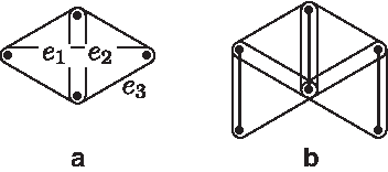
Three pairwise doubly incident 3-edges are called a doubly incident 3-edge-cycle (Fig. 4a). Figure 4b shows a hypergraph with a unique solution (depicted with bold 2-edges) which plays an important role in Lemma 6, which characterizes solutions for doubly connected components.

FIG. 4.

(a) Doubly incident 3-edge-cycle. (b) Forcing configuration of four doubly connected 3-edges.

Definition 11

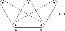
Let H be a hypergraph. A 3-edge-chain of length k is a subhypergraph of H composed of k 3-edges \documentclass{aastex}\usepackage{amsbsy}\usepackage{amsfonts}\usepackage{amssymb}\usepackage{bm}\usepackage{mathrsfs}\usepackage{pifont}\usepackage{stmaryrd}\usepackage{textcomp}\usepackage{portland, xspace}\usepackage{amsmath, amsxtra}\pagestyle{empty}\DeclareMathSizes{10}{9}{7}{6}\begin{document} $$e_1 = \{v_{1}, v_{2}, v_{3} \}, e_{2} = \{v_{2}, v_{3}, v_{4} \}, \ldots, e_{k} = \{v_{k}, v_{k + 1}, v_{k + 2} \}$$ \end{document} , where vertices \documentclass{aastex}\usepackage{amsbsy}\usepackage{amsfonts}\usepackage{amssymb}\usepackage{bm}\usepackage{mathrsfs}\usepackage{pifont}\usepackage{stmaryrd}\usepackage{textcomp}\usepackage{portland, xspace}\usepackage{amsmath, amsxtra}\pagestyle{empty}\DeclareMathSizes{10}{9}{7}{6}\begin{document} $$v_{1}, \ldots, v_{k + 2}$$ \end{document} are all distinct (Fig. 5). The vertices v₁ and v_k₊₂ are the end vertices of the chain.

FIG. 5.

Example of a 3-edge-chain of length k.

We have the following observation about solutions to the HC problem on 3-edge-chains.

Observation 4

If the input hypergraph for the HC problem is a 3-edge-chain \documentclass{aastex}\usepackage{amsbsy}\usepackage{amsfonts}\usepackage{amssymb}\usepackage{bm}\usepackage{mathrsfs}\usepackage{pifont}\usepackage{stmaryrd}\usepackage{textcomp}\usepackage{portland, xspace}\usepackage{amsmath, amsxtra}\pagestyle{empty}\DeclareMathSizes{10}{9}{7}{6}\begin{document} $$e_1 = \{v_{1}, v_{2}, v_{3} \}, e_{2} = \{v_{2}, v_{3}, v_{4} \}, \ldots, e_{k} = \{v_{k}, v_{k + 1}, v_{k + 2} \}$$ \end{document} , where k ≥ 3 then there are exactly two solutions. One solution consists of edges {(v_i, v_i₊₁); i is odd} and the other of edges {(v_i, v_i₊₁); i is even}. If k is odd then all but one of the end vertices are incident to an edge in both solutions. If k is even, in the first solution all vertices are incident to an edge, while in the second solution all but two end vertices are incident to an edge.

Lemma 6

Let H be a hypergraph with only 3-edges without doubly incident 3-edge-cycles such that every pair of vertices belongs to at most two 3-edges. If C contains the hypergraph depicted in Figure 4b then there is either no way or a unique way how to cover C. Otherwise, C is a 3-edge-chain.

Proof

First, if C has at most two 3-edges, it is a 3-edge-chain.

Second, consider a doubly connected set S with three 3-edges e₁, e₂, e₃. We may assume that e₁, e₂ (respectively, e₁, e₃) are doubly incident. Since, by assumption, e₂, e₃ are not doubly incident, we can assume that all doubly connected sets with three 3-edges form a 3-edge-chain (Fig. 6).

FIG. 6.

A 3-edge-chain.

Now, consider a doubly connected set S with four 3-edges. There are only four possibilities how this set can look like, depicted in Figure 7. In the first case, we have a 3-edge chain. In the second case, by Observation 3, there is either no covering or a unique covering of C. In the third and fourth cases there is no solution. Hence, we can assume that all doubly connected sets with four 3-edges form a 3-edge-chain. It follows that every doubly connected component is a 3-edge chain. ▪

FIG. 7.

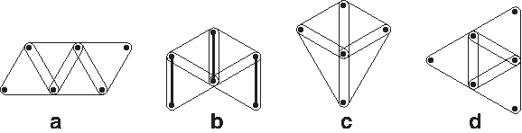
All possible cases for a doubly connected component with four 3-edges. The thick edges show the covering in case (b). In case (a) we have a 3-edge chain. In cases (c) and (d) there is no solution.

Now, we are ready to attack the HC problem in the general case.

Theorem 7

The HC problem can be solved in O(n(n + m)) time.

Proof

We give a polynomial algorithm for constructing a covering graph G with components of order at most 2 from an input hypergraph H. Initially, let G be the empty graph on vertices of H. First, we remove all 2-edges from H and place them to G. The algorithm will deal with the hyperedges of H one by one using a set of rules. Each processed hyperedge is removed from H and either

(T1) some pairs of vertices contained in the hyperedge are placed as edges to G so that the conditions of Definition 9 are satisfied, or

(T2) the choice for pairs of vertices from this hyperedge is postponed and binded to decision on the choice for another hyperedge still in H, or

(T3) an auxiliary hyperedge is added to H and the choice for pairs from the original hyperedge is binded to decision on the choice for this new hyperedge.

The first happens only if there is a unique choice for covering the processed hyperedge. Hence, in the moment when G contains two incident edges, it follows that there is no solution to the HC problem on H. It will be obvious from the algorithm that after applying all possible rules (in given order) either all hyperedges are processed, or all unprocessed edges are 3-edges, any two unprocessed hyperedges share at most one vertex and no unprocessed hyperedge and edge of G share a vertex. Hence, we can then apply the algorithm of Lemma 5 on the modified H (containing only unprocessed edges). Union of G and a solution from the algorithm of Lemma 5 gives a solution to the HC problem.

The set of rules:

1. If there is an hyperedge e contained in another hyperedge f, we proceed as in the case (T2). In particular, we remove e and bind the choice for pairs in e to the choice for pairs in f, i.e., covered pairs in e are exactly the pairs covered in f which are contained in e. From now on, we can assume that no hyperedge is contained in another.

2. If there is a pair of vertices u, v contained in at least three 3-edges, then remove all of them from H and add the edge (u, v) to G (Fig. 8).

3. If H contains doubly incident 3-edge-cycle (Fig. 4a), remove 3-edges of the cycle from H and add a new 4-edge into H consisting of the four vertices of the cycle. It is easy to see that this does not influence the solution.

4. For each 4-edge that intersect with other hyperedges in H or edge in G, its covering is uniquely determined or there is no covering for it and the algorithm fails. Consult Figure 9 for all possible cases.

(a) If two 4-edges share exactly one vertex, then there is no solution to the HC problem.

(b) If two 4-edges share exactly two vertices, remove them from H and add the pair of shared vertices as an edge to G. Furthermore, add the two remaining pairs (one per 4-edge) as edges to G. This results in covering of the two 4-edges.

(d) If a 4-edge shares exactly one vertex with a 3-edge e = {u, v, w}. Let u be the common vertex. Then remove e from H and add edge (v, w) to G.

(e) If a 4-edge shares exactly two vertices with a 3-edge, remove both of them from H and add the common pair together with the other disjoint pair of the 4-edge as edges to G.

(f) If a 4-edge shares exactly one vertex with a 2-edge in G, there is no solution.

After applying the above rules as many times as possible, the only 4-edges left in H are isolated from other hyperedges and also from edges in G. Hence, for each of them, we can arbitrarily pick covering pairs of edges and remove it from H. Thus, we can assume there are no 4-edges left in H.

5. If a 3-edge intersects a 2-edge in G in a single vertex, remove the 3-edge from H and add the edge formed by the remaining two vertices of the 3-edge to G. Apply this rule whenever a new edge is added to G.

6. Consider a doubly connected component C. By Lemma 6, either there is a unique or no way of covering C, or C is a 3-edge chain. In the former case, remove C from H and add 2-edges of the solution for C to G or return fail. Assume the second case. By Observation 4, if there is a 3-edge not in C containing an interval vertex of C, this 3-edge is uniquely covered. Hence, remove it from H and add the pair of its other two vertices as an edge to G. Now, all 3-edge chains can share only their end vertices.

FIG. 8.

The pair u, w contained in at least three 3-edges.

FIG. 9.

An 4-edge intersecting other hyperedges. The thick edges show the covering if it exists. In cases (a), (c), and (f ), there is no solution.

If a component C is a 3-edge-chain of even length, by Observation 4, there is a solution s for C which does not contain the end vertices (Fig. 10a). Covering C in this way will not affect the existence of the solution for H, since if there is a solution to H which contains the other solution for C then by replacing it with s results in a new solution which in addition has smaller number of edges. Hence, assume all doubly connected components are 3-edge-chains of odd length.

FIG. 10.

(a) An example of smaller solution to a 3-edge-chain of even length. (b) Replacement of a 3-edge-chain of odd length by a new 3-edge.

If there are two vertices which are end vertices of at least three 3-edge-chains, there is no solution. If there are two vertices which are end vertices of exactly two 3-edge-chains, then by Observation 4, there are only two solution for their union and each of them contains the two vertices. Hence, we can arbitrarily pick one of the solutions and add it to G and remove both 3-edge-chains from H.

Finally, we proceed as in case (T3): replace every 3-edge-chain by a 3-edge having the two end vertices u, v of the 3-edge-chain and one new vertex w (Fig. 10b). The solution for the 3-edge-chain is binded to the new 3-edge as follows: if the edge (u, v) is picked to cover the 3-edge, then cover the 3-edge-chain in any of the two possible ways; if the edge (u, w) is picked, cover the 3-edge-chain by the solution that contains u; and similarly for the edge (v, w).

After application of all rules above (which can be done in polynomial time), H will satisfy requirements of Lemma 5, and hence the solution can be found (if one exists) in polynomial time. Finally, the resolution of binded hyperedges can be done in polynomial time as well. To analyze the running time of the algorithm, let us look at individual steps. Steps 1–3 run in time O(n²), Steps 4 and 6 in O(n), and Step 5 in time O(nm). The algorithm of Lemma 5 takes time O(n²) and finally, resolution of binded hyperedges can be done in O(n) time. ▪

Note that the solution constructed by the above algorithm has the minimum number of edges; hence, the corresponding galled-tree network has the minimum number of recombinations.

To summarize the last phase, let us state the procedure inferring the genotype matrix A″.

Procedure 3. Inferring matrix using genotype hypergraph

1. Construct the genotype hypergraph for A″ (see Definition 9).

2. Use the algorithm described in Theorem 7 and Lemma 5 to find covering of the genotype hypergraph (with the minimal number of edges in the cover).

3. Using the covering determine how to infer every row with 2's.

Complexity analysis

The preprocessing which includes: determining values of indicators, listing of 2's in each row and computing the conflict graph of A, takes time O(nm²). Phase 1 takes time O(nm), Phase 2 O(n), and Phase 3 (solving HC problem) O(n² + nm). Thus, the algorithm runs in time O(n² + nm²).

3.5. Experimental results

We implemented the algorithm and performed the following experiments on simulation data. We compared our algorithm's performance with PHASE v2 (Stephens and Donnelly, 2003; Stephens et al., 2001). The results show that our algorithm seems promising for the corresponding haplotyping problem.

In particular, the data is prepared in three steps. First, binary matrices, each having a perfect phylogeny tree, are generated using Hudson's (Hudson, 2002) simulation program with recombination rate being 0. Then, for each matrix's perfect phylogeny tree, we randomly replace nodes on it with simple galls by adding new columns to matrices with each newly added column introducing a conflict between itself and an existing column in the matrix (thus, adding recombinations). Last, for each haplotype in the matrix, we randomly repeat it for two to six times and pair haplotypes to generate genotype matrices.

We infer haplotypes from the generated genotype matrices that have weak property using our algorithm and compare our algorithm's performance with PHASE base on three standards (Stephens et al., 2001): (1) the error rate, which is the proportion of genotypes having more than two 2's whose haplotypes are incorrectly inferred; (2) the discrepancy rate, which is the sum of frequency differences for each individual haplotypes (simulated or true ones); and (3) the switch accuracy (Lin et al., 2002) of the inferred haplotypes is defined as (h − w − 1)/(h − 1), where h is the number of 2's in a genotype g and w is the number of wrongly inferred 2's for g. Using Hudson's simulation algorithm and applying our random procedure to generate genotypes, we generated five sets of 100 matrices. The experimental results are shown in Table 1.

Table 1.

Comparison of Accuracy Between Our Algorithm (SGTN) and PHASE on the Five Sets of Matrices

	20^20*		30^20*		30^40*		100^50*		100^100*
	30^14*		45^16*		75^20*		199^33*		199^49*
	SGTN	PHASE	SGTN	PHASE	SGTN	PHASE	SGTN	PHASE	SGTN	PHASE
Error rate	0.005	0.008	0.012	0.013	0.002	0.000	0.007	0.002	0.002	0.001
Discrepancy	0.09	0.13	0.250	0.283	0.070	0.000	0.545	0.149	0.198	0.126
Switch accuracy	0.995	0.992	0.988	0.987	1	1	0.993	0.998	0.998	0.999
Time	0.54s	14.2s	0.49s	26.8s	0.43s	28.57s	0.83s	204s	2.95s	368.36s

The first row of the table lists the size of the matrices that were generated using Hudson program. The second row lists the average size of each group of matrices after applying our random algorithm and removed the duplated columns. Each rate is normalized by the number of genotype matrices in that set.

The results show that our algorithm have comparable accuracy with PHASE while runs tens to hundreds times faster.

4. Conclusions

We considered the problem of haplotyping via galled-tree networks introduced in Gusfield et al. (2004). We have shown that this problem can be solved in polynomial time for the input genotype matrices with the weak property and the galled-tree networks with two mutations per gall. Together with the result in Gupta et al. (2010) and preliminary results, where we showed that the problem is NP-complete if the size of galls (the number of mutation edges) is either not restricted or restricted to any k ≥ 3, we have determined the complexity of the problem depending on the number of mutations in galls. The remaining open problem is the complexity of the haplotyping via simple galled-tree networks for the genotype matrices without the weak property.

Footnotes

Disclosure Statement

No competing financial interests exist.

References

Bafna

, Gusfield

, Lancia

et al. 2003. Haplotyping as perfect phylogeny: a direct approach. J. Comput. Biol., 10:323–340.

Bonizzoni

, Vedova

G.D

, Dondi

et al. 2003. The haplotyping problem: an overview of computational models and solutions. J. Comput. Sci. Technol., 18:675–688.

Daly

, Rioux

, Schaffner

et al. 2001. High-resolution haplotype structure in the human genome. Nat. Genet., 29:229–232.

Gupta

, Maňuch

, Stacho

et al. 2006. Characterization of the existence of galled-tree networks. J. Bioinform. Comput. Biol., 4:1309–1328.

Gupta

, Maňuch

, Stacho

et al. 2007. Algorithm for haplotype inferring via galled-tree networks with simple galls (extended abstract) Lect. Notes Bioinform, 4463:121–132.

Gupta

, Maňuch

, Stacho

et al. 2009. Haplotype inferring via galled-tree networks using a hypergraph covering problem for special genotype matrices. Discrete Appl. Math., 157:2310–2324.

Gupta

, Karimi

, Maňuch

et al.(to appear)Haplotype inference via galled-tree networks is NP-complete. J. Comput. Biol., 17:1435–1449.

Gusfield

. 2002. Haplotyping as perfect phylogeny: conceptual framework and efficient solutions. Proc. RECOMB ’02, 166–175.

Gusfield

. 2004. An overview of combinatorial methods for haplotype inference. Lect. Notes Comput. Sci., 2983:9–25.

10.

Gusfield

. 2005. Optimal, efficient reconstruction of root-unknown phylogenetic networks with constrained and structured recombination. J. Comput. Syst. Sci., 70:381–398.

11.

Gusfield

, Orzack

S.H.

2005. Haplotype inference, 18–1–18–28. Handbook of Computational Molecular Biology. Chapman & Hall: London.

12.

Gusfield

, Eddhu

, Langley

. 2004. Optimal, efficient reconstruction of phylogenetic networks with constrained recombination. J. Bioinform. Comput. Biol., 2:173–213.

13.

Halldórsson

B.V

, Bafna

, Edwards

et al. 2004. A survey of computational methods for determining haplotypes. Lect. Notes Comput. Sci., 2983:26–47.

14.

Hein

. 1990. Reconstructing evolution of sequences subject to recombination using parsimony. Math. Biosci., 98:185–200.

15.

Hein

. 1993. A heuristic method to reconstruct the history of sequences subject to recombination. J. Mol. Evol., 36:396–405.

16.

Hudson

R.R

. 2002. Generating samples under a Wright-Fisher neutral model of genetic variation. Bioinformatics, 18:337–338.

17.

Lin

, Cutler

, Zwick

et al. 2002. Haplotype inference in random population samples. Am. J. Hum. Genet., 71:1129–1137.

18.

Mitra

R.D

, Butty

V.L

, Shendure

et al. 2003. Digital genotyping and haplotyping with polymerase colonies. Proc. Nat. Acad. Sci. USA, 100:5926–5931.

19.

Patil

, Berno

, Hinds

et al. 2001. Blocks of limited haplotype diversity revealed by high-resolution scanning of human chromosome 21. Science, 294:1719–1723.

20.

Song

, Hein

. 2003. On the minimum number of recombination events in the evolutionary history of DNA sequences. J. Math. Biol., 48:160–186.

21.

Song

Y.S

, Wu

, Gusfield

. 2005. Algorithms for imperfect phylogeny haplotyping (IPPH) with a single homoplasy or recombination event. Proc. WABI, 152–164.

22.

Sridhar

, Blelloch

G.E

, Ravi

et al. 2006. Optimal imperfect phylogeny reconstruction and haplotyping. Proc. Comput. Syst. Bioinform. Conf. (CSB06), 199–210.

23.

Stephens

, Donnelly

. 2003. A comparison of bayesian methods for haplotype reconstruction from population genotype data. Am. J. Hum. Genet., 73:1162–9.

24.

Stephens

, Smith

N.J

, Donnelly

. 2001. A new statistical method for haplotype reconstruction from population data. Am. J. Hum. Genet., 68:978–989.

25.

Wang

, Zhang

. 2001. Perfect phylogenetic networks with recombination. J. Comput. Biol., 8:69–78.