RNA Locally Optimal Secondary Structures

Abstract

RNA locally optimal secondary structures provide a concise and exhaustive description of all possible secondary structures of a given RNA sequence, and hence a very good representation of the RNA folding space. In this paper, we present an efficient algorithm that computes all locally optimal secondary structures for any folding model that takes into account the stability of helical regions. This algorithm is implemented in a software called regliss that runs on a publicly accessible web server.

1. Introduction

Noncoding RNAs (ncRNAs) play a wide range of roles in the cell (Mattick & Makunin, 2006), and for many of them, the function is mainly determined by their three-dimensional structure. A single stranded RNA folds upon itself to form base pairs, which shape the secondary structure of the molecule and act as a scaffold for the three-dimensional folding. Knowing the secondary structures is thus of critical importance to understanding the function of an RNA molecule. The earliest algorithms for the RNA folding problem appeared in the late 70s, see Eddy (2004) for a survey. Such algorithms take as input a single-stranded RNA sequence and output a single secondary structure possessing minimum free energy.

However, it became clear early on that computing the single minimum free-energy folding is not enough. For a number of reasons, the biologically correct structure is often not the optimal one, but rather a structure within a small percentage deviation of the minimum free energy. Firstly, slight changes in the thermodynamic model may produce very different foldings with a similar energy level. Secondly, the thermodynamic model does not allow for pseudoknots or base triplets, and it does not reflect the interactions of the RNA with other molecules in the cell. Thirdly, some biological processes involve switches, changes of conformation in RNA structures.

All of these reasons make it important to be able to predict multiple foldings, also called suboptimal foldings, that allow for a deeper insight at the RNA folding space. Moreover, being able to compute alternative structures may also be useful in designing RNA sequences, which not only have low folding energy, but whose folding landscape would suggest rapid and robust folding.

Several programs produce suboptimal foldings of RNA, including mfold/unafold (Zuker, 1989), RNAsubopt (Wuchty et al., 1999), and RNAshapes (Steffen et al., 2006). Unfortunately, as we will see in Section 2, none of these tools are fully suitable for an exhaustive enumeration of all possible secondary structures. To address this problem, Clote introduced the concept of locally optimal secondary structures (Clote, 2005a). A secondary structure is locally optimal if no base pairs can be added without creating a conflict, such as introducing a pseudoknot or a base triplet. The set of locally optimal secondary structures can be seen as a concise description of the space of all secondary structures, because each secondary structure is included in a locally optimal secondary structure. Clote proposed a dynamic programming algorithm to enumerate such structures. One drawback of this approach is that it uses the Nussinov-Jacobson model (Nussinov & Jacobson, 1980), which does not produce realistic secondary structures.

The problem of locally optimal secondary structures with an accurate folding model has been recently addressed in Lorenz & Clote (2011). The authors present an algorithm to compute the partition function over all locally optimal secondary structures of a given RNA sequence, extending the McCaskill's classical algorithm (McCaskill, 1990). This method, however, does not effectively produce the set of locally optimal secondary structures.

In this article, we introduce a novel approach to generate all locally optimal secondary structures assembled from a set of thermodynamically stable helices. We propose an efficient algorithm for this problem, which relies on decomposition of secondary structures into structures maximal for juxtaposition. As far as we know, this property has never been formulated or used to study locally optimal secondary structures. The article is organized as follows. Section 2 presents some background information on suboptimal and locally optimal secondary structures. Section 3 details our folding algorithms for the locally optimal structures. For pedagogical reasons, we first expose the main outlines of the algorithm for the simplistic Nussinov-Jacobson model (Section 3.1). We then explain how to adapt it to deal with thermodynamically stable helices (Section 3.2). Section 4 discusses the implementation. Finally, Section 5 presents some experimental results. All proofs are available in Supplementary Material, available online at www.liebertonline.com/cmb.

2. Background

In this section, we give a brief overview of the main suboptimal and locally optimal RNA folding methods.

Mfold/unafold (Zuker, 1989). The algorithm returns a sample set of the foldings by considering all possible base pairs and by computing the best folding that contains this base pair. The suboptimality level option further selects the suboptimal candidates to return only those within a given free energy range. The result is that not all possible structures need to be computed, which speeds up computational time. As a counterpart, even with 100% suboptimality level, the algorithm does not provide all possible suboptimal secondary structures. The number of calculated structures is intrinsically bounded by the number of possible base pairs. Whatever the suboptimality percentage is, it is quadratic in the length of the input sequence. By construction, secondary structures that contain at least “two different places” of suboptimality are not provided by the algorithm (Fig. 1, top). Another consequence is that the algorithm can output secondary structures that contain another secondary structure with a better free energy (Fig. 1, bottom).

FIG. 1.

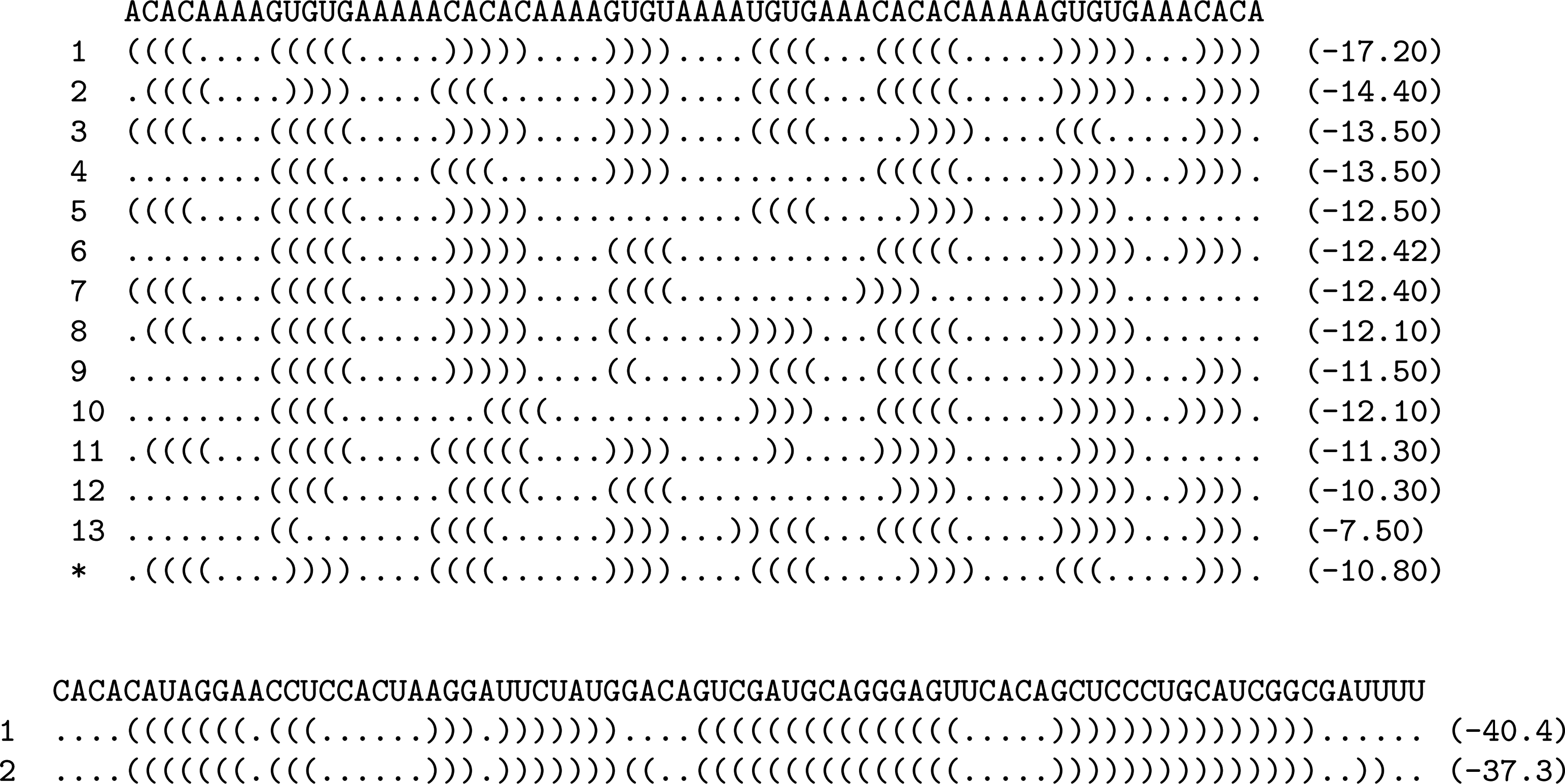
(Top) Unafold output on a toy sequence (64 nt) with 100% suboptimality. This software produces 13 suboptimal secondary structures, displayed in Vienna bracket-dot format, whose free energy ranges from −17.20 kcal/mol to −7.50 kcal/mol. It misses the structure * of free energy −10.80 kcal/mol, composed of four stem-loops. Each of these stem-loops has been identified by unafold (in structures #2 and #3), but the algorithm is not able to recover the four stem-loops in a same structure. (Bottom) Unafold output on sequence AY545598.5 (37939-38015), RF00107 (77 nt). Structure #2 contains structure #1, and has a higher energy level. Nevertheless, it is selected in the space of suboptimal structures, because it is the optimal structure containing base pair (33,75).

RNAsubopt (Wuchty et al., 1999). Another possibility to produce suboptimal structures is to modify the standard folding algorithm in order to output all secondary structures within a given energy range above the minimum free energy. However, if the threshold is set too low, not much variation is possible, and if it is set too high, too many structures may be generated for the reasonable evaluation. For example, the toy sequence of Figure 1 provides 4 structures within the energy range 10%, and 177 structures within the energy range 30%. The number of structures returned grows exponentially with both sequence length and energy range, and many structures are very similar.

RNAshapes (Steffen et al., 2006) organizes the suboptimal foldings to explore the folding space into classes of abstract shapes and reduces the potential exponential number of structures to a few classes. But two secondary structures with no common base pairs can be classified in the same shape.

Locally optimal secondary structures. The critical evaluation of these software programs suggests that there is a need of formal definitions for suboptimal secondary structures, which would correspond to local minima in the free energy landscape. The notions of saturated structures and locally optimal secondary structures meet this requirement. In Zuker and Sankoff (1984) and Evers and Giegerich (2001), a secondary structure is saturated when the stacking regions are extended maximally in both directions: No base pairs can be added at the extremity of a stacking region without degrading the free energy. Moreover, there is no isolated base pair.

In Clote (2005a), a secondary structure is locally optimal when no base pairs can be added without creating a conflict: either crossing pairings or a base triplet. The main drawback of Clote's result is that the algorithm relies on the Nussinov-Jacobson folding model. As a consequence, the number of locally optimal secondary structures is very large, and many of them are not thermodynamically stable in the nearest neighbor model. For example, the toy sequence of Figure 1 produces 1107 optimal secondary structures having 18 base pairs, 197,501 locally optimal secondary structures having 17 base pairs, and more than 6 million of locally optimal secondary structures having 16 base pairs. The work that we present here is inspired by this research. We start with the nice topological definition of locally optimal secondary structures, and extend it to take into account the stability of helical regions. In this context, locally optimal secondary structures are also saturated structures.

3. Algorithms

3.1. Folding at base pair resolution

We begin by considering locally optimal secondary structures for a simple model: All base pairs are independent, like in the Nussinov-Jacobson model. This model is mainly interesting for pedagogical purposes, because it allows us to provide basic definitions and ideas. We shall explain in Section 3.2 how to extend this to energetically stable helices to take into account interactions between adjacent base pairs.

3.1.1. Definitions

Let α be an RNA sequence of length n over the alphabet {A, C, G, U}: \documentclass{aastex}\usepackage{amsbsy}\usepackage{amsfonts}\usepackage{amssymb}\usepackage{bm}\usepackage{mathrsfs}\usepackage{pifont}\usepackage{stmaryrd}\usepackage{textcomp}\usepackage{portland, xspace}\usepackage{amsmath, amsxtra}\pagestyle{empty}\DeclareMathSizes{10}{9}{7}{6}\begin{document}$$\alpha = \alpha_1 \alpha_2 \ldots \alpha_n$$\end{document} . A base pair (x, y) on α is an ordered pair of natural numbers such that 1 ≤ x < y ≤ n. Base pairs are sorted according to the lexicographical order of their positions in the sequence: (x, y) is smaller than (z, t) if x < z, or if x = z and y < t. Given a set BP of base pairs on α, a structure is any subset of BP. We denote the empty structure by ɛ. A secondary structure on BP is a subset of BP such that any two distinct base pairs of S are either nested or juxtaposed:

• (x, y) is nested in (z, t) if z < x < y < t,

• (x, y) is juxtaposed with (z, t) if z < t < x < y.

The base pairs (x, y) and (z, t) are nested, if (x, y) is nested in (z, t) or (z, t) is nested in (x, y). The base pairs (x, y) and (z, t) are juxtaposed, if (x, y) is juxtaposed with (z, t) or (z, t) is juxtaposed with (x, y). Two base pairs that are neither nested nor juxtaposed are said to be conflicting.

Definition 1

Let S and T be two structures on BP. S is strictly included in T, or T is a strict extension of S, if any base pair of S is present in T, and there exists a base pair of T that is not in S.

Definition 2

Let S be a secondary structure on BP. S is locally optimal if it satisfies the following condition: If T is a structure that is strict extension of S, then T is not a secondary structure.

In other words, a secondary structure is locally optimal if no base pairs can be added without producing conflict. It follows that any secondary structure is included in a locally optimal structure. We give in Figure 2 an example of a set of base pairs and all its locally optimal secondary structures, which will serve as a running example throughout this paper.

FIG. 2.

Example and construction of locally optimal secondary structures. (a) The sequence has eight base pairs. (b) This set of base pairs contains 3 locally optimal secondary structures, {(1, 6), (2, 4), (7, 8), (9, 14), (10, 11), (12, 13)}, {(1, 6), (3, 5), (7, 8), (9, 14), (10, 11), (12, 13)} and {(2, 4), (5, 10), (7, 8), (12, 13)}. (c) It can form two structures maximal for juxtaposition, {(1, 6), (7, 8), (9, 14)} and {(2, 4), (5, 10), (12, 13)}. (d) The first structure maximal for juxtaposition extends to the two first locally optimal secondary structures. The second one extends to a single locally optimal secondary structure.

The set of all locally optimal secondary structures is potentially very large: It can be exponential in ℓ, the number of base pairs in BP. The exact upper bound, 3^ℓ/3, can be calculated by rephrasing the problem in terms of maximal independent sets. The set of vertices is BP and an edge links two conflicting base pairs. The locally optimal structures are exactly the maximal independent sets of the graph (see Fig. 1 in Supplementary Materials, available online at www.liebertonline.com/cmb.).

The idea of our algorithm is to reduce the combinatorics by taking advantage of properties of nested and juxtaposed relations, such as transitivity, to achieve a good running time in practice. We divide the construction of locally optimal structures into two steps: First applying only juxtaposition operations, then applying only nesting operations. Structures are thus decomposed into horizontal levels of juxtaposed base pairs. For that we need two more notations. Given a structure S, Toplevel(S) is defined as the set of base pairs of S that are not nested in any base pair of S. Given a base pair (x, y) in S, Nested(x, y, S) is the set of base pairs of S that are nested in (x, y) and that are not nested in any base pair nested in (x, y). These levels induce a partition of S: \documentclass{aastex}\usepackage{amsbsy}\usepackage{amsfonts}\usepackage{amssymb}\usepackage{bm}\usepackage{mathrsfs}\usepackage{pifont}\usepackage{stmaryrd}\usepackage{textcomp}\usepackage{portland, xspace}\usepackage{amsmath, amsxtra}\pagestyle{empty}\DeclareMathSizes{10}{9}{7}{6}\begin{document}$$S = {\rm Toplevel} ( S ) \cup \bigcup\nolimits_{ ( x , y ) \in S} { \rm Nested} ( x , y , S )$$\end{document} .

It is routine to verify that S is a secondary structure if, and only if, any two base pairs of Toplevel(S) are juxtaposed, and for each (x, y) of S, any two base pairs of Nested(x, y, S) are juxtaposed. One important result for our algorithm is that the property for a secondary structure to be locally optimal can be testified by looking only at the Toplevel and Nested subsets. We will show that these subsets must be maximal for juxtaposition.

Definition 3

Let S be a structure on BP. S is maximal for juxtaposition if it satisfies the two following conditions:

(i) if b and b′ are two distinct base pairs in S, then b and b′ are juxtaposed,

(ii) if b is a base pair of BP not present in S such that {b} ∪ S is a secondary structure, then b is nested in some base pair of S.

Figure 2c gives examples of structures maximal for juxtaposition. The link between structures maximal for juxtaposition and locally optimal secondary structures is established by Theorem 1.

Theorem 1

A structure S on BP is a locally optimal secondary structure if, and only if,

(i) Toplevel(S) is maximal for juxtaposition on BP[1 . n],

(ii) for each base pair (x, y) of S, Nested(x, y, S) is maximal for juxtaposition in BP[x+1 . y−1]

BP[x . y] denotes the subset of BP composed of base pairs (z, t) such that x ≤ z < t ≤ y. The proof of Theorem 1 is given in Supplementary Materials, available online at www.liebertonline.com/cmb. Figure 2d gives an illustration of the Theorem.

3.1.2. Construction of structures maximal for juxtaposition

We show how to efficiently construct the structures maximal for juxtaposition. For each pair of positions i and j of α, we define the set of secondary structures MJ(i, j) as follows.

1. If i ≥ j, then MJ(i, j) = {ɛ}

2. otherwise, if there is no base pair (i, y), i < y ≤ j, in BP, then MJ(i, j) = MJ(i + 1, j)

3. otherwise

\documentclass{aastex}\usepackage{amsbsy}\usepackage{amsfonts}\usepackage{amssymb}\usepackage{bm}\usepackage{mathrsfs}\usepackage{pifont}\usepackage{stmaryrd}\usepackage{textcomp}\usepackage{portland, xspace}\usepackage{amsmath, amsxtra}\pagestyle{empty}\DeclareMathSizes{10}{9}{7}{6}\begin{document}\begin{align*}\qquad\qquad\qquad\qquad\qquad{\rm MJ} ( i , j ) = \bigcup \begin{cases} \bigcup_{ ( i , y ) \in {\rm BP} [ i.j ] } \{ ( i , y ) \} \bigoplus {\rm MJ} ( y + 1 , j ) & \qquad\qquad\qquad\qquad\quad( a) \\ \\ \bigcap_{ ( i , y ) \in {\rm BP} [ i.j ] } Filter ( ( i , y ) , {\rm MJ} ( i + 1 , j ) ) & \qquad\qquad\qquad\qquad\quad ( b) \end{cases}\end{align*}\end{document}

The operator ⨁ denotes the concatenation of a base pair to a set of structures: S is in {(i, y)} ⨁ MJ(y + 1, j) if, and only if, there exists S′ in MJ(y+1, j) such that S = {(i, y)} ∪ S′. In rule 3b, a Filter function is used to check the maximality of structures. It is defined as follows: Given a base pair b, and a set of secondary structures R, the secondary structure S of R is in Filter(b, R) if, and only if, there exists a base pair b′ in S such that b and b′ are conflicting. We have the following Theorem.

Theorem 2

Let i and j be two positions on α. MJ(i, j) is exactly the set of all structures maximal for juxtaposition on BP[i . j].

The question is now how to implement the formula to compute MJ(i, j). The recurrence relation naturally suggests to use dynamic programming with a two-dimensional table, indexed by i and j. This can be further refined. A close inspection of Theorem 1 shows that not all pairs of positions i and j are useful for the computation of locally optimal secondary structures: We only need MJ(x+1,y−1) for all base pairs (x, y) of BP, and intermediate values necessary to obtain MJ(x+1, y−1). So we should only consider pairs of positions of the form (k,y−1) with x<k<y and (x, y) in BP. The last point that we want to make here is that in the rule 3b, the computation of Filter((x, y),MJ(i, j)) requires at most O(y − x) tests for every structure \documentclass{aastex}\usepackage{amsbsy}\usepackage{amsfonts}\usepackage{amssymb}\usepackage{bm}\usepackage{mathrsfs}\usepackage{pifont}\usepackage{stmaryrd}\usepackage{textcomp}\usepackage{portland, xspace}\usepackage{amsmath, amsxtra}\pagestyle{empty}\DeclareMathSizes{10}{9}{7}{6}\begin{document}$$S \in {\rm MJ} ( i , j )$$\end{document} . Indeed, given a structure S in MJ(i, j), let b be the first base pair of S not nested in (x, y). S belongs to Filter((x, y), MJ(i, j)) if, and only if, such a b exists and is conflicting with (x, y).

3.1.3. Construction of locally optimal secondary structures

We now explain how to compute the set of locally optimal secondary structures from the set of structures maximal for juxtaposition. The stepping stone is Theorem 1, stated in Section 3.1.1. This result allows us to view the set of locally optimal secondary structures as the set of ordered rooted tree whose vertices are labeled by structures maximal for juxtaposition. More precisely, each tree is such that:

• The root is labeled by an element of MJ(1, n),

• Each node is labeled by an element w of MJ(x+1, y−1) for some base pair (x, y) of BP,

• The out-degree of a node labeled by w is the number of base pairs of w,

• The ith child of a node labeled by w is labeled by an element of MJ(x+1, y−1), where (x, y) is the ith base pair of w.

Figure 3b gives the three possible trees for the locally optimal secondary structures of the example of Figure 2. This representation brings an effective way to compute all locally optimal secondary structures. The enumeration of all possible such trees can be done easily with a push-down stack whose elements are structures maximal for juxtaposition. The pseudo-code of the algorithm is given in Figure 4, and an example of a run is given in Figure 3c. At each iteration of the algorithm, the stack contains a different locally optimal secondary structure. The height of the stack is bounded by ℓ′, the maximal number of structures maximal for juxtaposition present in the locally optimal secondary structure. This value is much smaller than the number of base pairs of the output structure, and thus smaller than the total size of BP. Each iteration of the loop is then done in time O(ℓ′). Subsequently, the construction of all locally secondary structures can be performed in time linear in the size of the output, that is the total number of base pairs of all locally optimal secondary structures.

FIG. 3.

(a) Locally optimal secondary structures of Figure 3. (b) Associated ordered trees. MJ(i, j)[k] denotes the kth element of MJ(i, j). (c) Content of the stack at the end of each iteration of the algorithm of Figure 5 (lines 5, 6, and 7). MJ(i,j)[k] is now symbolized by the triplet (i, j, k). Each cell of the stack corresponds to an internal node of the underlying tree depicted in (b). For example, at iteration 1, the line 5 pushes the triplet (1, 14, 0), corresponding to MJ(1,14)[0] = {(1, 6), (7, 8), (9,14)}, then the nested structures are pushed.

FIG. 4.

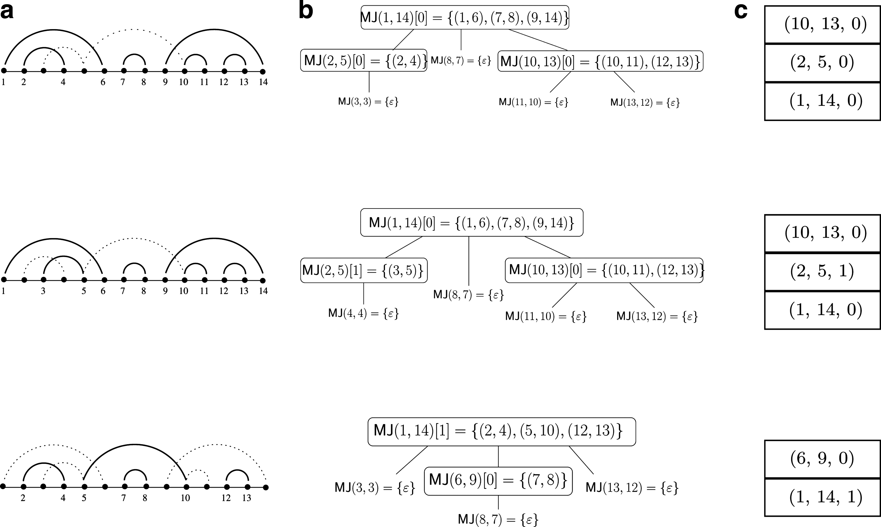
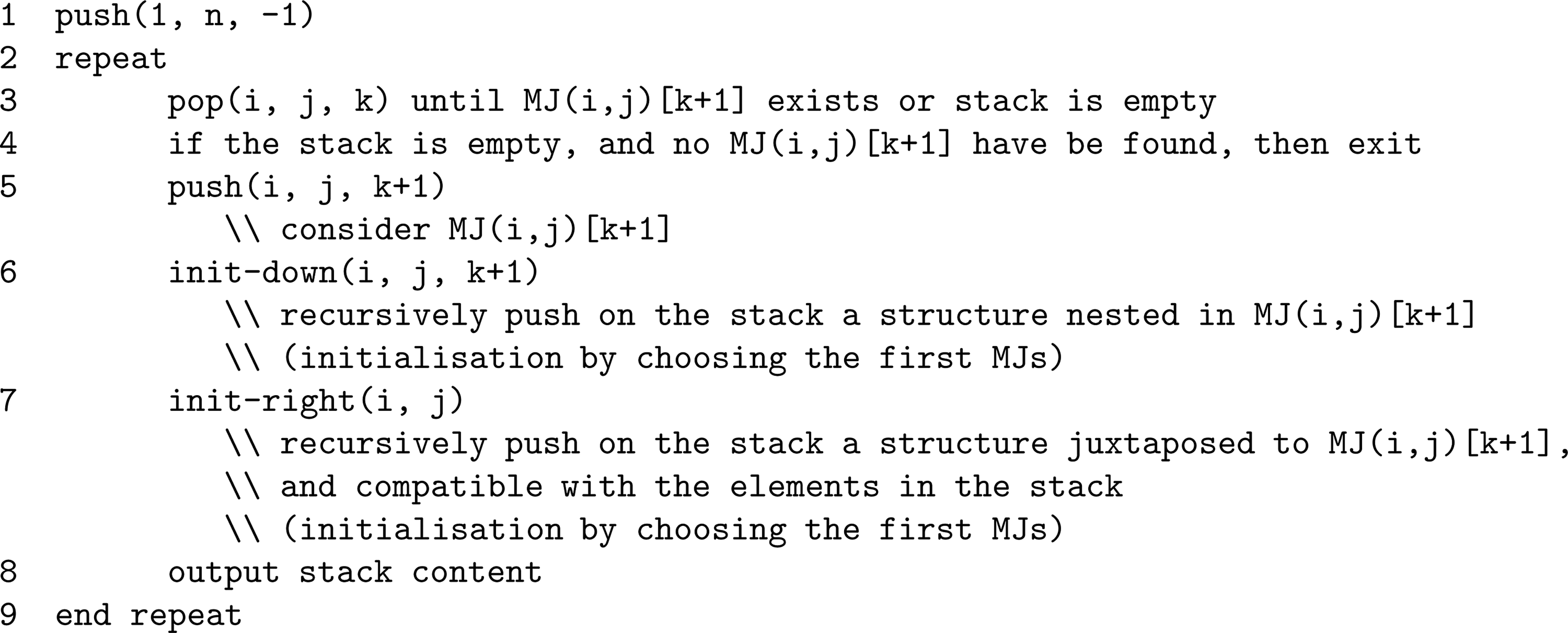
Enumeration of all locally optimal secondary structures from the set of all structures maximal for juxtaposition. Each iteration of the loop outputs one locally optimal structure. MJ(i, j)[k] denotes the kth element of MJ(i, j).

3.1.4. Back to Clote's algorithm

In Section 2, we mentioned the seminal work of Clote (2005a) on counting locally optimal secondary structures for the Nussinov-Jacobson model. This work uses a clever optimization based on the notion of visible bases and visible positions. Given a secondary structure S, a visible position p in S is a position outside any base pair of S: \documentclass{aastex}\usepackage{amsbsy}\usepackage{amsfonts}\usepackage{amssymb}\usepackage{bm}\usepackage{mathrsfs}\usepackage{pifont}\usepackage{stmaryrd}\usepackage{textcomp}\usepackage{portland, xspace}\usepackage{amsmath, amsxtra}\pagestyle{empty}\DeclareMathSizes{10}{9}{7}{6}\begin{document}$$\forall ( x , y ) \in S$$\end{document} , p < x ∨ y < p. By extension, a character \documentclass{aastex}\usepackage{amsbsy}\usepackage{amsfonts}\usepackage{amssymb}\usepackage{bm}\usepackage{mathrsfs}\usepackage{pifont}\usepackage{stmaryrd}\usepackage{textcomp}\usepackage{portland, xspace}\usepackage{amsmath, amsxtra}\pagestyle{empty}\DeclareMathSizes{10}{9}{7}{6}\begin{document}$$c \in \{ A , C , G , U \} $$\end{document} is visible in S if there exists a visible position p such that c = α_p. Let v ⊂{A, C, G, U} be a subset of the alphabet, and let Loc(i, j)[v] be the set of locally optimal structures between positions i and j, where the bases v, and only these bases, are visible. Then Loc(i, j), the set of all locally optimal structures between positions i and j, is the union of the different Loc(i, j)[v] for all v ⊂{A, C, G, U}.

Let's now fix a given set of allowed pairings. For example, one can consider only Watson-Crick base pairs, taking for BP (the set of possible base pairs) the following WC set: \documentclass{aastex}\usepackage{amsbsy}\usepackage{amsfonts}\usepackage{amssymb}\usepackage{bm}\usepackage{mathrsfs}\usepackage{pifont}\usepackage{stmaryrd}\usepackage{textcomp}\usepackage{portland, xspace}\usepackage{amsmath, amsxtra}\pagestyle{empty}\DeclareMathSizes{10}{9}{7}{6}\begin{document}\begin{align*}{\rm WC} = \{ ( x , y ) \mid 1 \le x < y \le n \ { \rm and} \ ( \{ \alpha_x , \alpha_y \} = \{ A , U \} \ { \rm or } \ \{ \alpha_x , \alpha_y \} = \{ C , G \} ) \} \end{align*}\end{document}

The sets of locally optimal structures can then be computed in a very efficient way: \documentclass{aastex}\usepackage{amsbsy}\usepackage{amsfonts}\usepackage{amssymb}\usepackage{bm}\usepackage{mathrsfs}\usepackage{pifont}\usepackage{stmaryrd}\usepackage{textcomp}\usepackage{portland, xspace}\usepackage{amsmath, amsxtra}\pagestyle{empty}\DeclareMathSizes{10}{9}{7}{6}\begin{document}\begin{align*}Loc ( i , j ) [ {\bf v} ] = \bigcup \begin{cases} \bigcup_{ ( i , y ) \in {\rm WC} [ i.j ] } \{ ( i , y ) \} \bigoplus Loc ( i + 1 , y - 1 ) \bigoplus Loc ( y + 1 , j ) [ {\bf v} ] \\ \\ Loc ( i + 1 , j ) [ {\bf v} - \{ \overline{ \alpha_i} \} ] \cup Loc ( i + 1 , j ) [ {\bf v} - \{ \alpha_i , \overline{ \alpha_i} \} ] \end{cases}\end{align*}\end{document}

In the second line, \documentclass{aastex}\usepackage{amsbsy}\usepackage{amsfonts}\usepackage{amssymb}\usepackage{bm}\usepackage{mathrsfs}\usepackage{pifont}\usepackage{stmaryrd}\usepackage{textcomp}\usepackage{portland, xspace}\usepackage{amsmath, amsxtra}\pagestyle{empty}\DeclareMathSizes{10}{9}{7}{6}\begin{document}$$\overline{ \alpha_i}$$\end{document} is the complementary base of α_i. As this base \documentclass{aastex}\usepackage{amsbsy}\usepackage{amsfonts}\usepackage{amssymb}\usepackage{bm}\usepackage{mathrsfs}\usepackage{pifont}\usepackage{stmaryrd}\usepackage{textcomp}\usepackage{portland, xspace}\usepackage{amsmath, amsxtra}\pagestyle{empty}\DeclareMathSizes{10}{9}{7}{6}\begin{document}$$\overline{ \alpha_i}$$\end{document} is never visible in the locally optimal structures in \documentclass{aastex}\usepackage{amsbsy}\usepackage{amsfonts}\usepackage{amssymb}\usepackage{bm}\usepackage{mathrsfs}\usepackage{pifont}\usepackage{stmaryrd}\usepackage{textcomp}\usepackage{portland, xspace}\usepackage{amsmath, amsxtra}\pagestyle{empty}\DeclareMathSizes{10}{9}{7}{6}\begin{document}$$Loc ( i + 1 , j ) [ { \bf v} - \{ \overline{ \alpha_i} \} ]$$\end{document} and \documentclass{aastex}\usepackage{amsbsy}\usepackage{amsfonts}\usepackage{amssymb}\usepackage{bm}\usepackage{mathrsfs}\usepackage{pifont}\usepackage{stmaryrd}\usepackage{textcomp}\usepackage{portland, xspace}\usepackage{amsmath, amsxtra}\pagestyle{empty}\DeclareMathSizes{10}{9}{7}{6}\begin{document}$$Loc ( i + 1 , j ) [ { \bf v} - \{ \alpha_i , \overline{ \alpha_i} \} ]$$\end{document} , that guarantees that all such structures are also locally optimal on WC[i . j] : no Filter function is further required.

It is possible to take advantage of this optimization and to combine it with our construction method through structures maximal for juxtaposition. We obtain the following recurrence relation for this construction: \documentclass{aastex}\usepackage{amsbsy}\usepackage{amsfonts}\usepackage{amssymb}\usepackage{bm}\usepackage{mathrsfs}\usepackage{pifont}\usepackage{stmaryrd}\usepackage{textcomp}\usepackage{portland, xspace}\usepackage{amsmath, amsxtra}\pagestyle{empty}\DeclareMathSizes{10}{9}{7}{6}\begin{document}\begin{align*}{\rm MJ} ( i , j ) [ {\bf v} ] = \bigcup \begin{cases} \bigcup_{ ( i , y ) \in {\rm WC} [ i.j ] } \{ ( i , y ) \} \bigoplus {\rm MJ} ( y + 1 , j ) [ {\bf v} ] \\ \\ {\rm MJ} ( i + 1 , j ) [ {\bf v} - \{ \overline{ \alpha_i} \} ] \cup {\rm MJ} ( i + 1 , j ) [ {\bf v} - \{ \alpha_i , \overline{ \alpha_i} \} ] \end{cases}\end{align*}\end{document}

The construction of locally optimal secondary structures from structures maximal for juxtaposition (as described in Theorem 1) is then unchanged. The same optimization can be adapted to some larger BP sets, including, for example, the wobble G-U pairs. However, the efficiency of the method relies on a set of fixed base pairs, independently of their positions: our algorithm allows far more flexibility, constructing locally optimal structures on any initial set of base pairs BP.

3.2. Folding at helix resolution

In this section, we extend the construction of locally optimal secondary structures to the framework of energetically favorable helices. This model is likely to produce more biologically realistic structures, because it takes into account the stacking energy between base pairs, such as introduced in the nearest neighbor model (Matthews et al., 1999), for example.

3.2.1. Definitions

We admit a generic definition for helices. It is an ordered set of base pairs \documentclass{aastex}\usepackage{amsbsy}\usepackage{amsfonts}\usepackage{amssymb}\usepackage{bm}\usepackage{mathrsfs}\usepackage{pifont}\usepackage{stmaryrd}\usepackage{textcomp}\usepackage{portland, xspace}\usepackage{amsmath, amsxtra}\pagestyle{empty}\DeclareMathSizes{10}{9}{7}{6}\begin{document}$$\{ ( x_1 , y_1 ) , \ldots , ( x_k , y_k ) \} $$\end{document} such that \documentclass{aastex}\usepackage{amsbsy}\usepackage{amsfonts}\usepackage{amssymb}\usepackage{bm}\usepackage{mathrsfs}\usepackage{pifont}\usepackage{stmaryrd}\usepackage{textcomp}\usepackage{portland, xspace}\usepackage{amsmath, amsxtra}\pagestyle{empty}\DeclareMathSizes{10}{9}{7}{6}\begin{document}$$x_1 < \ldots < x_k$$\end{document} , and \documentclass{aastex}\usepackage{amsbsy}\usepackage{amsfonts}\usepackage{amssymb}\usepackage{bm}\usepackage{mathrsfs}\usepackage{pifont}\usepackage{stmaryrd}\usepackage{textcomp}\usepackage{portland, xspace}\usepackage{amsmath, amsxtra}\pagestyle{empty}\DeclareMathSizes{10}{9}{7}{6}\begin{document}$$y_1 > \ldots > y_k$$\end{document} . It can contain bulges and internal loops. The 5′ arm of the helix is the set of positions \documentclass{aastex}\usepackage{amsbsy}\usepackage{amsfonts}\usepackage{amssymb}\usepackage{bm}\usepackage{mathrsfs}\usepackage{pifont}\usepackage{stmaryrd}\usepackage{textcomp}\usepackage{portland, xspace}\usepackage{amsmath, amsxtra}\pagestyle{empty}\DeclareMathSizes{10}{9}{7}{6}\begin{document}$$x_1 , \ldots , x_k$$\end{document} , and the 3′ arm is the set of positions \documentclass{aastex}\usepackage{amsbsy}\usepackage{amsfonts}\usepackage{amssymb}\usepackage{bm}\usepackage{mathrsfs}\usepackage{pifont}\usepackage{stmaryrd}\usepackage{textcomp}\usepackage{portland, xspace}\usepackage{amsmath, amsxtra}\pagestyle{empty}\DeclareMathSizes{10}{9}{7}{6}\begin{document}$$y_1 , \ldots , y_k$$\end{document} . We denote by f.5start, f.5end, f.3start, and f.3end the first position of the 5′ arm, the last position of the 5′ arm, the first position of the 3′ arm, and the last position of the 3′ arm, respectively. Given two distinct helices f and g, we define four different relations between f and g:

• g is nested in f if f.5end < g.5start and g.3end < f.3start (in this case, any base pair of g is nested in any base pair of f),

• g is juxtaposed with f if f.3end < g.5start (in this case, any base pair of g is juxtaposed with any base pair of f),

• g is embedded in f if any base pair of g is also a base pair of f,

• otherwise, f and g are said to be conflicting.

The concepts of structures, secondary structures, strict inclusion (Definition 1), and locally optimal secondary structures (Definition 2) on base pairs can easily be adapted to helices:

• A structure is any subset of H. Given a structure S on BP, S is described by the structure \documentclass{aastex}\usepackage{amsbsy}\usepackage{amsfonts}\usepackage{amssymb}\usepackage{bm}\usepackage{mathrsfs}\usepackage{pifont}\usepackage{stmaryrd}\usepackage{textcomp}\usepackage{portland, xspace}\usepackage{amsmath, amsxtra}\pagestyle{empty}\DeclareMathSizes{10}{9}{7}{6}\begin{document}$$\{ f_1 , \ldots , f_k \} $$\end{document} on H, if \documentclass{aastex}\usepackage{amsbsy}\usepackage{amsfonts}\usepackage{amssymb}\usepackage{bm}\usepackage{mathrsfs}\usepackage{pifont}\usepackage{stmaryrd}\usepackage{textcomp}\usepackage{portland, xspace}\usepackage{amsmath, amsxtra}\pagestyle{empty}\DeclareMathSizes{10}{9}{7}{6}\begin{document}$$S = f_1 \cup \cdots \cup f_k$$\end{document} .

• A secondary structure is any subset of H such that any two helices are either nested or juxtaposed.

• Given two structures \documentclass{aastex}\usepackage{amsbsy}\usepackage{amsfonts}\usepackage{amssymb}\usepackage{bm}\usepackage{mathrsfs}\usepackage{pifont}\usepackage{stmaryrd}\usepackage{textcomp}\usepackage{portland, xspace}\usepackage{amsmath, amsxtra}\pagestyle{empty}\DeclareMathSizes{10}{9}{7}{6}\begin{document}$$\{ f_1 , \ldots , f_k \} $$\end{document} and \documentclass{aastex}\usepackage{amsbsy}\usepackage{amsfonts}\usepackage{amssymb}\usepackage{bm}\usepackage{mathrsfs}\usepackage{pifont}\usepackage{stmaryrd}\usepackage{textcomp}\usepackage{portland, xspace}\usepackage{amsmath, amsxtra}\pagestyle{empty}\DeclareMathSizes{10}{9}{7}{6}\begin{document}$$\{ g_1 , \ldots , g_j \} $$\end{document} of H, we say that \documentclass{aastex}\usepackage{amsbsy}\usepackage{amsfonts}\usepackage{amssymb}\usepackage{bm}\usepackage{mathrsfs}\usepackage{pifont}\usepackage{stmaryrd}\usepackage{textcomp}\usepackage{portland, xspace}\usepackage{amsmath, amsxtra}\pagestyle{empty}\DeclareMathSizes{10}{9}{7}{6}\begin{document}$$\{ f_1 , \ldots , f_k \} $$\end{document} is strictly included in \documentclass{aastex}\usepackage{amsbsy}\usepackage{amsfonts}\usepackage{amssymb}\usepackage{bm}\usepackage{mathrsfs}\usepackage{pifont}\usepackage{stmaryrd}\usepackage{textcomp}\usepackage{portland, xspace}\usepackage{amsmath, amsxtra}\pagestyle{empty}\DeclareMathSizes{10}{9}{7}{6}\begin{document}$$\{ g_1 , \ldots , g_j \} $$\end{document} if the set of base pairs \documentclass{aastex}\usepackage{amsbsy}\usepackage{amsfonts}\usepackage{amssymb}\usepackage{bm}\usepackage{mathrsfs}\usepackage{pifont}\usepackage{stmaryrd}\usepackage{textcomp}\usepackage{portland, xspace}\usepackage{amsmath, amsxtra}\pagestyle{empty}\DeclareMathSizes{10}{9}{7}{6}\begin{document}$$f_1 \cup \cdots \cup f_k$$\end{document} is strictly included in \documentclass{aastex}\usepackage{amsbsy}\usepackage{amsfonts}\usepackage{amssymb}\usepackage{bm}\usepackage{mathrsfs}\usepackage{pifont}\usepackage{stmaryrd}\usepackage{textcomp}\usepackage{portland, xspace}\usepackage{amsmath, amsxtra}\pagestyle{empty}\DeclareMathSizes{10}{9}{7}{6}\begin{document}$$g_1 \cup \cdots \cup g_j$$\end{document} .

• A secondary structure \documentclass{aastex}\usepackage{amsbsy}\usepackage{amsfonts}\usepackage{amssymb}\usepackage{bm}\usepackage{mathrsfs}\usepackage{pifont}\usepackage{stmaryrd}\usepackage{textcomp}\usepackage{portland, xspace}\usepackage{amsmath, amsxtra}\pagestyle{empty}\DeclareMathSizes{10}{9}{7}{6}\begin{document}$$\{ f_1 , \ldots , f_k \} $$\end{document} of H is locally optimal if it satisfies the following condition: If \documentclass{aastex}\usepackage{amsbsy}\usepackage{amsfonts}\usepackage{amssymb}\usepackage{bm}\usepackage{mathrsfs}\usepackage{pifont}\usepackage{stmaryrd}\usepackage{textcomp}\usepackage{portland, xspace}\usepackage{amsmath, amsxtra}\pagestyle{empty}\DeclareMathSizes{10}{9}{7}{6}\begin{document}$$\{ g_1 , \ldots , g_j \} $$\end{document} is a structure on H that is a strict extension of \documentclass{aastex}\usepackage{amsbsy}\usepackage{amsfonts}\usepackage{amssymb}\usepackage{bm}\usepackage{mathrsfs}\usepackage{pifont}\usepackage{stmaryrd}\usepackage{textcomp}\usepackage{portland, xspace}\usepackage{amsmath, amsxtra}\pagestyle{empty}\DeclareMathSizes{10}{9}{7}{6}\begin{document}$$\{ f_1 , \ldots , f_k \} $$\end{document} , then \documentclass{aastex}\usepackage{amsbsy}\usepackage{amsfonts}\usepackage{amssymb}\usepackage{bm}\usepackage{mathrsfs}\usepackage{pifont}\usepackage{stmaryrd}\usepackage{textcomp}\usepackage{portland, xspace}\usepackage{amsmath, amsxtra}\pagestyle{empty}\DeclareMathSizes{10}{9}{7}{6}\begin{document}$$\{ g_1 , \ldots , g_j \} $$\end{document} is not a secondary structure on H.

From now on, we assume that we have a set H of helices of size ℓ, and we work with structures defined on H. We also assume that helices of H are ranked from 1 to ℓ according to a total helix ordering <, and that the order verifies f < g ⇒ f.5start < g.5start. Given two helices f and g in H, H[f.g] denotes the subset of H composed of helices whose all base pairs are in the interval [f.5start.g.3end], and H]f.g[ the subset of H composed of helices whose all base pairs are in the interval ]f.5end.g.3start[. As before, for a structure F on H, Toplevel(F) is defined as the set of helices of F that are not nested in any helix of F, and Nested(f, F) is the set of helices of F that are nested in the helix F and that are not nested in any helix nested in f.

We now turn to the problem of constructing all locally optimal secondary structures for a set of helices. The two-step method described in Section 3.1 is still valid: First considering structures maximal for juxtaposition and constructing them by dynamic programming, then recovering locally optimal secondary structures on the fly with a push-down stack. However, the algorithm needs some adaptation to take into account the existence of embedded helices and the fact that some helices can combine to form other helices present in the input set.

3.2.2. Construction of structures maximal for juxtaposition

Definition 3 for base pairs can be adapted to helices.

Definition 4

Given a set of helices H, and a structure F on H, F is maximal for juxtaposition if it satisfies the two following conditions:

(i) if f and g are two distinct helices of F, then f and g are juxtaposed,

(ii) if f is a helix of H not present in F such that {f} ∪ F is a secondary structure on H, then f is nested in some helix of F.

As in Section 3.1, we define for each pair of helices f and g of H a set of secondary structures MJ(f,g) that contains all structures maximal for juxtaposition for H[f.g].

1. If f.5start > g.3end, then MJ(f,g) = {ɛ}

2. otherwise, if f.3end > g.3end, then MJ(f,g) = MJ(f + 1,g)

3. otherwise

\documentclass{aastex}\usepackage{amsbsy}\usepackage{amsfonts}\usepackage{amssymb}\usepackage{bm}\usepackage{mathrsfs}\usepackage{pifont}\usepackage{stmaryrd}\usepackage{textcomp}\usepackage{portland, xspace}\usepackage{amsmath, amsxtra}\pagestyle{empty}\DeclareMathSizes{10}{9}{7}{6}\begin{document}\begin{align*}\qquad\qquad\qquad\qquad\qquad{\rm MJ} ( f , g ) = \bigcup \begin{cases} \{ f \} \bigoplus {\rm MJ} (\hbox{next Juxt} ( f ) , g ) & \qquad\qquad\qquad\qquad\qquad\qquad \quad(3a) \\ \\ Filter ( f , {\rm MJ} ( f + 1 , g ) ) & \qquad\qquad\qquad\qquad\qquad\quad\qquad( 3b) \end{cases}\end{align*}\end{document}

Now ⨁ denotes the concatenation of a helix to a set of structures, f + 1 denotes the next helix (wrt the helix ordering) after f, and nextJuxt(f) denotes the smallest helix (wrt the helix ordering) juxtaposed with f. The definition of Filter is a straightforward translation from the definition on base pairs to helices: Given a helix h and a set of secondary structures R on H, the secondary structure S of R is in Filter(h,R) if, and only if, there exists a helix h′ in S such that h and h′ are neither nested nor juxtaposed. We then have a result analogous to the Theorem 2.

Theorem 3

For each pair of helices f and g of H, MJ(f, g) is exactly the set of structures maximal for juxtaposition on H[f.g].

3.2.3. Construction of locally optimal secondary structures

The construction of locally optimal secondary structures must take into account the fact that different sets of helices can describe the same base pair secondary structure in some cases. This happens when two nested helices can combine to form a new helix (Fig. 5, left). Of course, the algorithm should output only one structure. To address this problem, we introduce the definition of strong nestedness. Intuitively, two helices of are strongly nested, if each time they occur simultaneously in a locally optimal secondary structure, they can be merged into a single helix.

FIG. 5.

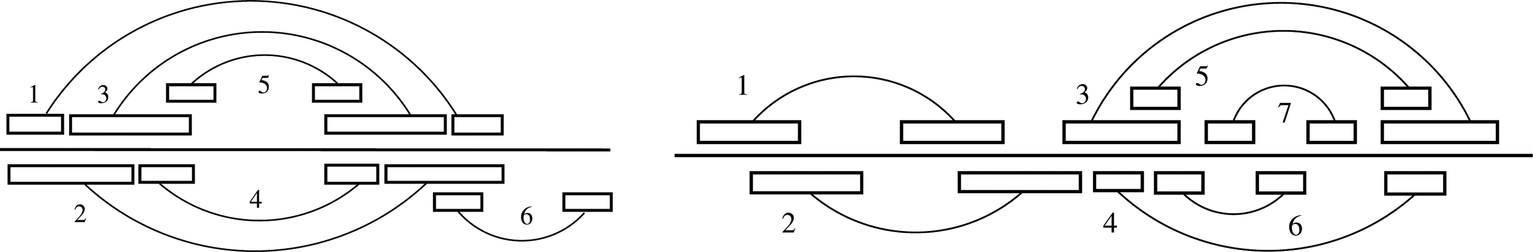
(Left) This helix set contains six helices, numbered from 1 to 6. The union of helices 1 and 3 gives the same set of base pairs as the union of helices 2 and 4. Thus {1,3} and {2,4} are two descriptions of the same structure of base pairs. Helix 3 is strongly nested in helix 1, and helix 4 is strongly nested in helix 2. The closure is obtained by adding the helix 1 ∪ 3. The locally optimal secondary structures are {1 ∪ 3}, {2,5}, {4,6}, and {5,6}. (Right) Structures maximal for juxtaposition and locally optimal secondary structures on helices. The set of helices H contains seven elements, ranked according to a helix ordering. Helix 5 is embedded in helix 3. There are five structures maximal for juxtaposition for H[1.3]: {1, 3}, {1, 4}, {1, 5}, {2, 4}, {2, 5}. There are six locally optimal secondary structures: {1, 3, 7}, {1, 4, 6}, {1, 4, 7}, {2, 4, 6}, {2, 4, 7}, {2, 5, 7}. Importantly, the structure {1, 5, 7} is not locally optimal, even if its substructures at Toplevel and Nested levels are maximal for juxtaposition. The reason is that it is strictly included in {1, 3, 7}.

Definition 5

Let f and g be two helices, such that g is nested in f. Helix g is strongly nested in f, if for any helix h that is either juxtaposed with g, or in which g is nested, then h is not nested in f. The set of helices H is closed under strong nestedness if, for any two helices f and g of H such that g is strongly nested in f, then f ∪ g is also in H.

For any set of helices H, it is easy to construct its closure under strong nestedness by iteratively adding a new helix obtained by merging two strongly nested helices until the set is closed (Fig. 5, left). The set of locally optimal secondary structures is unchanged. From now on, we assume that the set of input helices H is closed under strong nestedness. In this context, we show that each locally optimal secondary structure can be written in a unique way as the combination of helices that are mutually not strongly nested. We call such structures canonical structures.

Definition 6

A structure F is canonical if any two helices of F are not strongly nested.

Property 1

Let H be a set of helices closed under strong nestedness, and let G be a locally optimal secondary structure on H. There exists a unique canonical structure F, such that F and G describe the same base pairs structure.

So the problem of computing all locally optimal secondary structures reduces to construct all canonical locally optimal secondary structures. How to solve it? In Section 3.1, we saw that locally optimal secondary structures for base pairs could be obtained exactly from structures maximal for juxtaposition. Here, each locally optimal secondary structure can still be decomposed into levels of helices that are maximal for juxtaposition. However, the reciprocal result is no longer true. Figure 5, right, shows an example where some combination of structures maximal for juxtaposition gives a secondary structure that is not locally optimal. This fact comes from the existence of embedded helices. So we have to identify which combinations of structures maximal for juxtaposition lead to locally optimal secondary structures. With canonical secondary structures, the local optimality could be established by looking at all helices not present in the structure. This allows us to formulate a simple condition that guarantees that a given helix in a secondary structure cannot be replaced by an embedding helix.

Definition 7

Let f be a helix of H, and T be a subset of H. We say that f fulfills the condition (⋆) in T, if for any helix h of H such that f is embedded in h, h is conflicting with some helix of T.

In Figure 5b, the helix 5 does not fulfill the condition (⋆) in the structure {1,5,7}, as the helix 3 is not conflicting with any helix of the structure. Finally, Theorem 1 on base pairs is replaced by Theorem 4 on helices.

Theorem 4

Let F be a canonical secondary structure on H. F is locally optimal if, and only if, it fulfills the two following properties:

(i) Toplevel(F) is maximal for juxtaposition,

(ii) for each helix f of F, Nested(f, F) is maximal for juxtaposition on H]f.f[, Nested(f, F) is not a single helix, and f fulfills the condition (⋆) in F.

It follows that the construction of locally optimal secondary structures from the sets of structures maximal for juxtaposition can be performed using the same algorithm described in Section 3.1.3 and in Figure 4, based on a push-down stack whose elements are structures maximal for juxtaposition. The only difference, at line 5 (push of an element) and at lines 6 and 7 (push of nested and juxtaposed structures), is that structures containing exactly one helix (Condition (ii)b of Theorem 4), and the structures that do not meet the (⋆) condition (Condition (ii)c of Theorem 4) are not pushed on the stack.

4. Implementation and Availability

The algorithm for locally optimal secondary structures with helices was implemented in C in a software called regliss (standing for RNA energy landscape and secondary structures). It is freely available on the regliss server. The input of regliss is an RNA sequence together with a set of putative helices given by the user. The helices can also be computed directly by the server from the RNA sequence. The output is the set of all locally optimal structures, sorted according to the free energy as computed with rnaeval (Hofacker et al., 1994). We also produce an energy landscape graph, useful for visualizing at a glance all found structures.

Running times. We show in Table 1 the running times of regliss for a selection of RNA sequences. The program was run on an Athlon Core 2 Duo with 2 GB RAM. The running time mainly depends of the number of output structures. When there are only some one hundred stuctures, regliss runs almost instantaneoulsy. However, as the number of structures can be exponential in the number of putative helices, regliss can be longer for some sequences.

Table 1.

Running Times and Output Size of Regliss for Some RNA Sequences

Sequence family	Species	Sequence length	Number of helices	Number of structures	Running time
tRNA – RF00005	S. pombe	76 nt	54	511	<0.2 s
GcvB – RF00022	Enterobacter sp.1	208 nt	62	3663	0.08 s
SRP-euk-arch – RF00017	M. voltae	298 nt	76	49775	0.62 s
RNase P – RF00010	P. marinus	405 nt	76	93142	1.49 s
5S rRNA – RF00001	D. radiophilus	119 nt	124	304059	2.51 s
RNase P – RF00010	S. usitatus	358 nt	104	1071968	20.92 s

5. Experimentations

5.1. Example on a SECIS element

Selenocysteine insertion sequence (SECIS) elements occur in messenger RNAs encoding selenoproteins (Walczak et al., 1996) and direct the cell machinery to translate UGA (Uracil, Guanine, Adenine) stop codons as selenocysteines. They are around 60 nucleotides in length and that adopt a stem-loop structure. Here we work with sequence Y11109.1/1272-1330, from Oreochromis niloticus (RFAM RF00031; Gardner et al., 2009). We first ran unafold asking “all” suboptimal structures (100% suboptimality, option -P 100). This gives 30 structures, displayed in Figure 6. The expected consensus secondary structure is not present in this set of structures. We also observe that several predictions are redundant: structure #2 is a strict extension of structure #1, structures #4 and #6 are both strict extensions of structure #3, and structure #20 is a strict extension of structure #11. We kept all nonredundant structures, and from them we extracted all putative helices. By doing so, we obtained 39 helices and launched regliss on this helix set. Regliss generates 192 locally optimal secondary structures. Structure #14 found by regliss is consistent with the consensus structure provided in RFAM for this family.

FIG. 6.

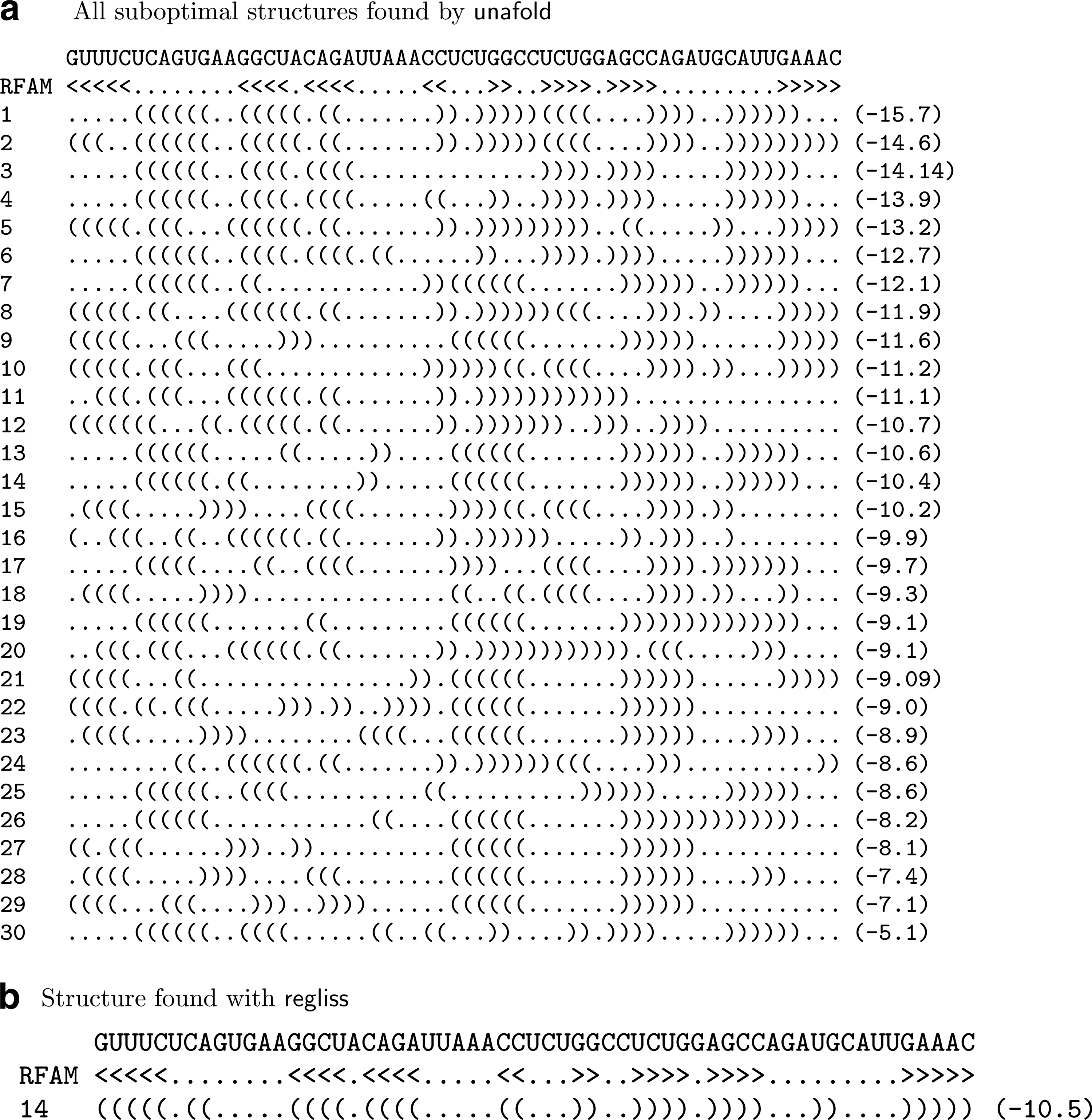
Results for SECIS element (Y11109.1/1272-1330). (a) Unafold results, all structures. (b) Structure #14, not found by unafold and found by regliss.

5.2. Comparison between regliss and unafold

We generalized the experiment of the previous paragraph, analyzing the size of the output of regliss and comparing it to unafold on a large number of RNA sequences from RFAM database. We selected all families of RFAM having sequences shorter than 200 nt, then picked up five sequences randomly for each family. This gives 5308 sequences. As in the preceding example, we run unafold with 100% suboptimality, and we provide regliss with helices coming from non redundant suboptimal unafold structures. Figure 7 shows the number of structures found with regliss compared to the theoretical upper bound of Section 3.1.1, as well as the number of structures produced by unafold on the same data. As expected, unafold generates at most a quadratic number of suboptimal structures, even with a 100%-suboptimality level, whereas regliss produces an exponential number of locally optimal structures.

FIG. 7.

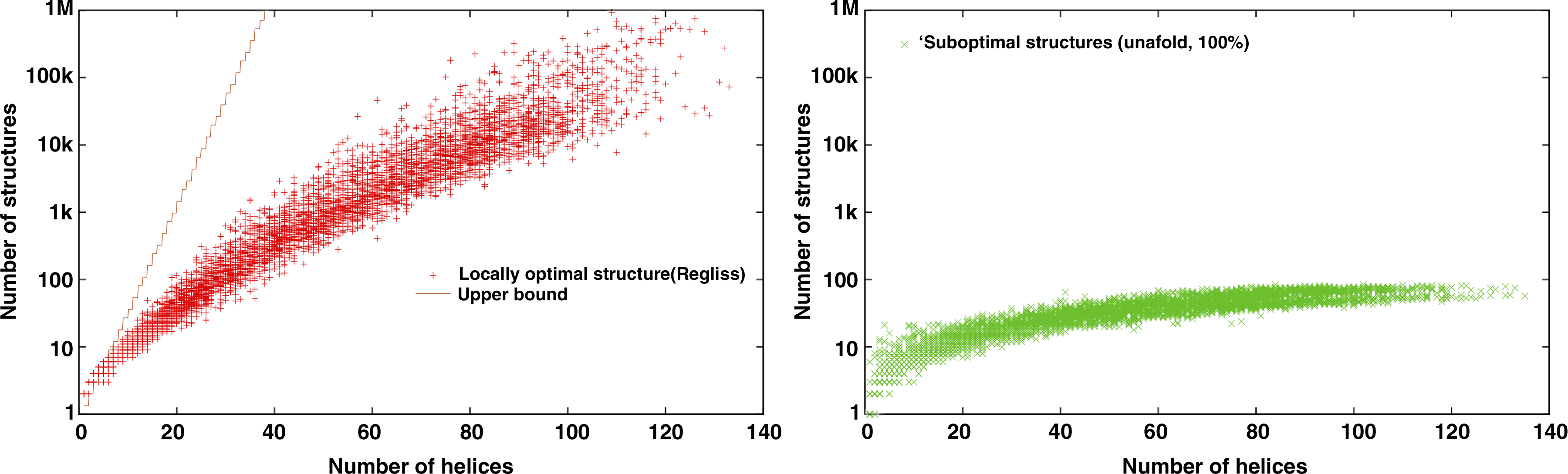
(Left) Number of structures produced by regliss on 5308 sequences from RFAM. The line is the 3^l/3 theoretical upper bound. On average, there are 2.98 times more locally optimal structures than structures maximal for juxtaposition. (Right) Number of structures produced by unafold (100% suboptimality) on the same set of helices. The unafold software never generates more than 84 structures.

We then evaluated the free energy of each structure with rnaeval and selected structures whose energy is greater than or equal to 80% of the optimal energy (we call them “20%-suboptimality structures”). The 5308 sequences divide in three groups:

• 10% sequences: unafold finds more structures than regliss. Typically, some of these structures are redundant, and are discarded by regliss;

• 25% sequences: unafold and regliss find the same number of 20%-suboptimality structures. In this group, almost all sequences have few putative helices and consequently a very small number of 20%-suboptimality structures (1205 sequences have at most 10 different 20%-suboptimality structures). Both programs often find exactly the same 20%-suboptimality structures;

• 65% sequences: regliss finds more 20%-suboptimality structures than unafold and so offers a larger variety of structures.

5.3. Structured versus random sequences

In Clote (2005a), it is proved that for some families, structured RNA has a different folding landscape than random RNA of the same dinucleotide frequency. We reproduce here this experimentation using regliss. We used the sequence of a Hammerhead type III ribozyme sequence that is also used in Clote (2005a). For this sequence, we generated 100 randomized sequences with the same length and the same dinucleotide composition. This computation has been performed with the dishuffle program, which implements the dinucleotide shuffle algorithm described in Altschul and Erickson (1985). We then compared the distributions of locally optimal secondary structures between these randomized sequences and the initial sequence. The result is shown in Figure 8. Graphs obtained with regliss are even more convincing than those obtained with RNALOSS. Figure 8 also shows graphs obtained on a 5S rRNA and on a tRNA sequence. Again, these tend to confirm that the folding landcapes, seen as the distribution of locally optimal structures, are different between structured RNAs and random sequences.

FIG. 8.

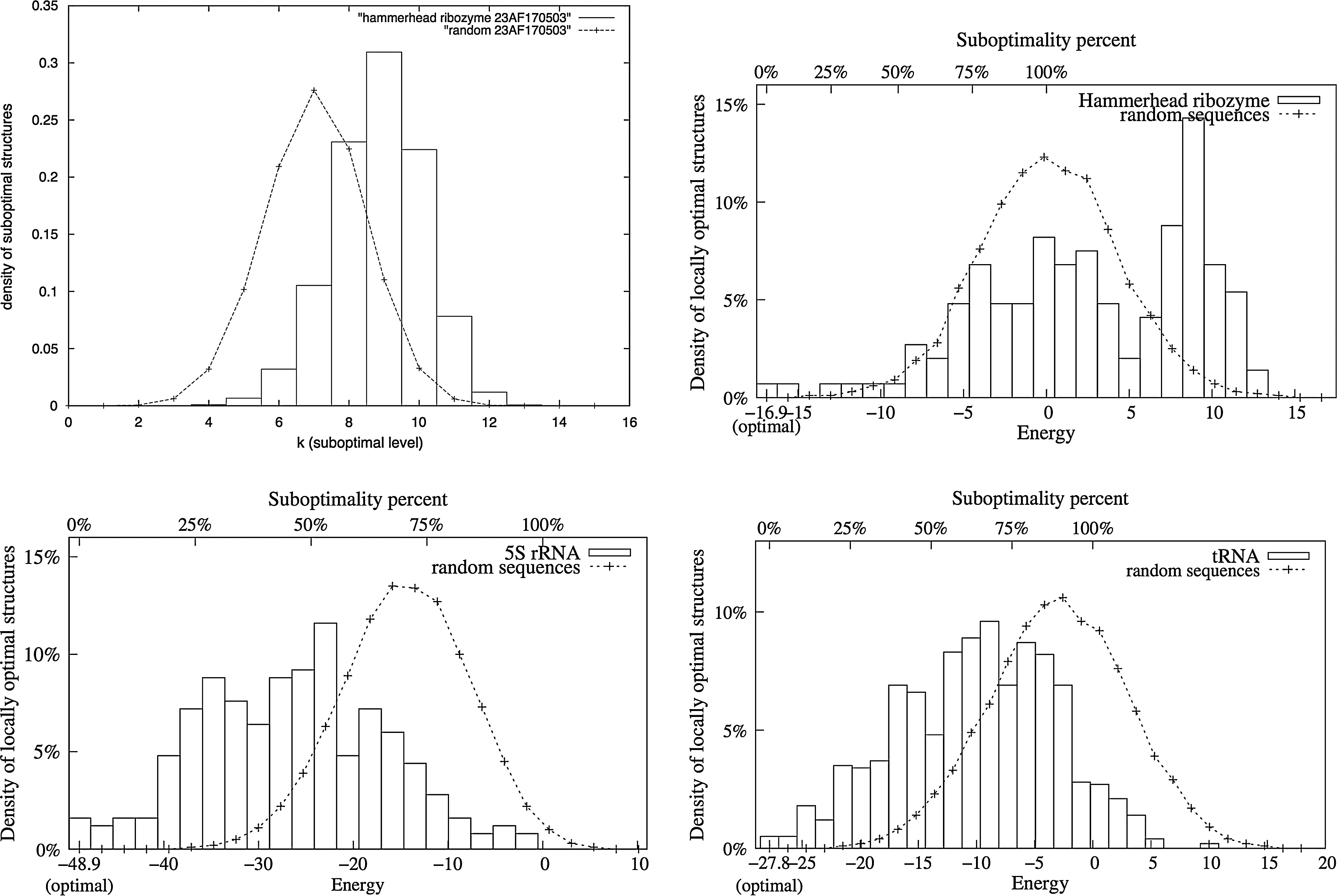
(Top) Density of locally optimal secondary structures of Hammerhead type III ribozyme (54 nt,RFAM RF0008, AF170503) versus average density off all locally optimal secondary structures of 100 random RNAs of same dinucleotide frequency and same length. (Left) RNALOSS results (figure from Clote, 2005a). (Right) Regliss results. (Below) Same experiment with 5S rRNA (RFAM RF00001, DQ397844.1/16860-16979) and tRNA (E.coli, PDB_00313).

6. Conclusion

We introduced a novel approach to produce locally optimal secondary structures of an RNA sequence, which enables us to break down the complexity of the problem into simpler steps. This work shows that all locally optimal secondary structures of a given RNA can effectively be computed. From a practical point of view, these structures can also be filtered out using some post-processing criterium, such as the free energy or the shape of the structure. This is a fruitful alternative to existing software programs, and the set of locally optimal secondary structures brings a new look into the folding space of an RNA sequence. Another advantage of the method is that the user can provide its own set of helices, based on the thermodynamic nearest neighbor model or any other model.

Footnotes

Disclosure Statement

No competing financial interests exist.

References

Altschul

S.F.

, Erickson

B.W.

1985. Significance of nucleotide sequence alignments: a method for random sequence permutation that preserves dinucleotide and codon usage. Molecular Biology and Evolution, 2:526–38.

Clote

2005a. An efficient algorithm to compute the landscape of locally optimal RNA secondary structures with respect to the Nussinov-Jacobson energy model. J. Computational Biology, 1:83–101.

Eddy

S.R.

2004. How do RNA folding algorithms work? Nat. Biotechnol, 22:1457–1458.

Evers

D.J.

, Giegerich

2001. Reducing the Conformation Space in RNA Structure Prediction. Presented at the German Conference on Bioinformatics, Braunschweig, Germany.

Gardner

P.P.

, Daub

, Tate

J.G.

et al. 2009. Rfam: updates to the RNA families database. Nucleic Acids Research, 37:D136–D140.

Hofacker

I.L.

, Fontana

, Stadler

P.F.

et al. 1994. Fast Folding and Comparison of RNA Secondary Structures. Monatshefte f. Chemie., 125:167–188.

Lorenz

W.A.

, Clote

2011. Computing the Partition Function for Kinetically Trapped RNA Secondary Structures. PLoS ONE, 6:e16178.

Matthews

D.H.

, Sabrina

, Zuker

et al. 1999. Expanded sequence dependence of thermodynamic parameters improves prediction of RNA secondary structure. J. Mol. Biol., 288:911–940.

Mattick

J.S.

, Makunin

I.V.

2006. Non-coding RNA. Hum Mol Genet, 15:R17–29.

10.

McCaskill

1990. The equilibrium partition function and base pair binding probabilities for RNA secondary structure. Biopolymers, 29:11051119.

11.

Moon

, Moser

1965. On cliques in graphs. Israel Journal of Mathematics, 3:23–28.

12.

Nussinov

, Jacobson

A.B.

1980. Fast algorithm for predicting the secondary structure of single-stranded RNA. Proc. Nat. Acad. Sci. USA. Biochemistry, 77:6309–6313.

13.

Steffen

, Voss

, Rehmsmeier

et al. 2006. RNAshapes: an integrated RNA analysis package based on abstract shapes. Bioinformatics, 22:500–503.

14.

Walczak

, Westhof

, Carbon

et al. 1996. A novel RNA structural motif in the selenocysteine insertion element of eukaryotic selenoprotein mRNAs. RNA, 2:367–379.

15.

Wuchty

, Fontana

, Hofacker

I.L

et al. 1999. Complete suboptimal folding of RNA and the stability of secondary structures. Biopolymers, 49:145–165.

16.

Zuker

1989. On finding all suboptimal foldings of an RNA molecule. Science, 244,4900:48–52.

17.

Zuker

, Sankoff

1984. RNA secondary structures and their prediction. Bulletin of Mathematical Biology, 46:591–621.

Supplementary Material

Please find the following supplemental material available below.

For Open Access articles published under a Creative Commons License, all supplemental material carries the same license as the article it is associated with.

For non-Open Access articles published, all supplemental material carries a non-exclusive license, and permission requests for re-use of supplemental material or any part of supplemental material shall be sent directly to the copyright owner as specified in the copyright notice associated with the article.

0.00 MB

0.09 MB