Gene Prediction Based on DNA Spectral Analysis: A Literature Review

Abstract

The identification of regions of DNA sequences that code for proteins is one of the most fundamental applications in bioinformatics. These protein-coding regions are in contrast to other DNA regions that encode functional RNA molecules, provide structural stability of chromosomes, serve as genetic raw materials, represent molecular fossils, or have no known purpose (sometimes called “junk DNA”). A number of approaches have been suggested for differentiating between the protein-coding and non-protein-coding regions of DNA. A selection of these approaches is based on digital signal processing (DSP) techniques. These DSP techniques rely on the phenomenon that protein-coding regions have a prominent power spectrum peak at frequency f = ⅓ arising from the length of codons (three nucleic acids). This article partitions the identification of protein-coding regions into four discrete steps. Based on this partitioning, DSP techniques can be easily described and compared based on their unique implementations of the processing steps. We compare the approaches, and discuss strengths and weaknesses of each in the context of different applications. Our work provides an accessible introduction and comparative review of DSP methods for the identification of protein-coding regions. Additionally, by breaking down the approaches into four steps, we suggest new combinations that may be worthy of future study.

1. Introduction

Genomic sequences consist of intergenic spacers and genes. For a long time, there was no known function for intergenic regions. However, recently it has been found that intergenic regions are not only junk regions, but they include many genes. These genes are called non-coding ribonucleic acids (ncRNAs), which do not code for proteins, but have other roles in different processes. They affect transcriptional regulation, chromosome structure, RNA processing and modification, gene splicing, and the stability and translation of messenger RNA, which is protein-coding RNA (Eddy, 2001; Storz, 2002). There are different classes of ncRNA, including microRNA (miRNA), small interfacing RNA (siRNA), and small nuclear RNA (snRNA) (Eddy, 2001). Protein-coding genes are responsible for protein synthesis, so they are called coding regions. Typically, intergenic spacers constitute about 95% of a genomic strand (Akhtar et al., 2008a). In the human genome, protein-coding genes constitute 2% of the total DNA (Akhtar et al., 2008b; Gibbs, 2003). In prokaryotes, coding genes are not separated by protein non-coding regions (introns). However, in eukaryotes, protein-coding regions that are also called exons are interrupted by protein non-coding regions, called introns (Akhtar et al., 2008a; Vaidyanathan and Yoon, 2002; Fox and Carreira, 2004). This article reviews methods that have been proposed to mainly identify protein-coding regions in eukaryotes. Since we are interested in studying methods in the scope of the identification of protein-coding regions, in this article we call these regions “coding-regions” and all other ncRNA regions “non-coding regions.”

Exonic regions code for amino acids. There are 20 amino acids in living cells. George Gamow proposed that there should be three bases that code for a protein amino acid, since 3 is the smallest integer n, such that 4ⁿ is at least 20 (Nanjundiah, 2004; Crick, 1988). The standard genetic code defines a mapping between the tri-nucleotide sequences and protein amino acids. According to this mapping, exonic regions are logically divided into groups of three bases, and each group of three bases is called a triplet or codon since a codon codes for a protein amino acid. There are 64 combinations of codons, which means some amino acids are redundantly coded by more than one codon (Cristea, 2002; Vaidyanathan and Yoon, 2002).

Predicting exons is important to know the primary structure of the protein that is synthesized by these exons. Learning the primary structure of a protein leads to studying and analyzing the secondary and tertiary structures of a protein in addition to protein function. Studying and analyzing the structure and function of a protein is important to design drugs, cure diseases, improve crop productivity, and synthesize biofuel (Nemati et al., 2009). In addition, coding regions represent the conserved part of genomes. Predicting conserved regions is important to study evolution and predict phylogenetic trees.

With the significant growth of sequenced genomic data, it has become important to come up with computerized methods for gene prediction. The productivity of the manual methods does not accommodate the accumulated sequenced genomes. Moreover, these methods require the intervention of experts in the process. Automatic and computational methods have been proposed to accelerate the gene prediction process. DSP has proved its success in different fields, and bioinformatics is one of these fields. DSP tools like the discrete Fourier transform (DFT) have been used to analyze DNA sequences. Gene prediction is one of the bioinformatics applications that have been implemented using the DFT. It has been observed that there is a prominent power spectrum peak at frequency f = ⅓ in the coding regions of a DNA sequence, and no such peak can be observed in non-coding regions (Chechetkin and Turygin, 1995; Tsonis et al., 1991; Fickett, 1982). This characteristic has also been called period-3 property or 3-base periodicity. Researchers have stated that the prominence of this peak at frequency f = ⅓ (period τ = 3) in coding regions is related to the nucleotide triplet arrangement (or codon) that encodes protein amino acids (Voss, 1992). Some researchers have attributed the existence of period-3 property in coding regions to the biased usage of codons in coding regions and the fact that proteins normally exhibit specific amino acid compositions (Tsonis et al., 1991; Fickett, 1982). Based on a variety of numerical experiments, Tiwari et al. (1997), however, proposed that while the biased usage of codons plays an important role in the existence of period-3 property, it is not the main reason of the existence of this property. Their experiments propose that this property could be a result of the amino acid sequence in natural proteins which expresses itself as a biased usage of certain triplets in coding regions of DNA sequences.

Most of the gene prediction techniques that are based on DSP analysis follow a sequence of common, specific steps in analyzing symbolic DNA sequences to predict coding regions. Figure 1 shows the block diagram of the generic gene prediction process based on the DSP analysis. We, therefore, propose that the process be broken down into four main components. Dividing the process into these components makes reviewing, comparing and contrasting papers proposed in this field more objective and easier. In addition, researchers in this field can address the weaknesses of their methods and work on improving the efficacy of each component of the process. The first component in the process is to convert symbolic DNA sequences into numerical sequences since DSP tools can process only numerical entities. Symbolic DNA sequences are mapped to numerical sequences while retaining the biological meaning of the represented information. The second step involves determining how sequences are processed. Some techniques process sequences based on a window, and the window shape and length are important parameters here (Akhtar et al., 2008b,c). The third stage, the analysis tool, is the most important component in the process. In this step, the period-3 component is extracted from DNA sequences to differentiate between coding and non-coding regions. This step could also include post-processing of the period-3 signal to improve the prediction accuracy. Finally, the last step is the classification of the resulting period-3 signals into coding and non-coding regions. Signal classification could include machine learning or be based on a threshold value.

FIG. 1.

The block diagram of the gene prediction process based on the spectral analysis of DNA sequences. The dashed line means that, in some methods, a sequence itself could be used in the classification stage to compute the threshold value intrinsically. A training data could be used in the analysis stage when a gene prediction method includes training.

In order to process DNA sequences by DSP tools, biomolecular sequences should be converted from a symbolic form into a numerical form. Several representation schemes have been proposed for this task (Bielinska-Waz et al., 2007; Yau et al., 2003; Voss, 1992). The Voss representation scheme is one of the most popular schemes used to map symbolic DNA sequences to numerical sequences (Voss, 1992). In this method, a DNA sequence is mapped to four binary indicator sequences corresponding to the four nucleotides. In each binary indicator sequence, the existence of a particular nucleotide in a relative base pair position is replaced by 1 and the absence of the nucleotide is replaced by 0 (Voss, 1992). Some methods map a DNA sequence into a complex-valued form (Cristea, 2002), while other methods replace each nucleotide with a 2D vector (Yau et al., 2003).

The windowing system of processing DNA sequences for coding region prediction is different from one technique to another. Most of the techniques analyze DNA sequences based on a walking window basis. According to the window basis, a rectangular window or any other shape with a specific length of base pairs is processed at a time. Then the window is slid by one or more base pair positions along the sequence, and the processing is repeated on that window until the end of the sequence. It has been shown that the window shape and length parameters affect the prediction results (Akhtar et al., 2008b,c; Liew et al., 2005; Li and Holste, 2005).

Researchers have used DSP tools to design gene prediction methods that use the period-3 property to discriminate between coding and non-coding regions. One of these tools is the short time Fourier transform (STFT) which has been used to compute the power spectrum peak at frequency f = ⅓ in DNA sequences (Tiwari et al., 1997; Anastassiou, 2000). The STFT processes a DNA sequence based on a sliding window basis. A DNA sequence is mapped to a numerical sequence, and a sliding window with a specific length L is shifted along the sequence. Each time the sliding window is shifted by one or more base pair positions, the power spectrum at frequency L/3 is computed in order to extract the period-3 property of the sequence (Tiwari et al., 1997). Digital filtering is another DSP tool that has been used in processing DNA sequences to extract the period-3 property (Vaidyanathan and Yoon, 2002). Digital filters centered at frequency 2π/3 are designed to extract the period-3 component.

Some gene prediction techniques are data-driven, which means these techniques rely on training or statistical data in the design of the analysis-tool stage. In these techniques, model parameters are tuned based on data used in a training or optimization process; in addition, these parameters could be calculated based on compositional statistics of data. Studies of computational gene prediction techniques (Makarov, 2002; Rogic et al., 2001) show that data-driven techniques depend more on compositional statistics of genomic sequences than the sequences themselves. High prediction accuracy can be attributed to friendly training and testing genomic data (Akhtar et al., 2008a). Therefore, the model might not be adaptive enough to work on data from various sources (organisms). Akhtar et al. (2008a) postulate that a system combining improved DSP techniques with existing data-driven techniques could provide a coding region prediction accuracy higher than that offered by the existing data-driven techniques alone.

After extracting the period-3 property, sequences are classified as coding and non-coding regions. Classification can be performed using a learning approach or a threshold. Thresholding is considered one of the major challenges in this field since the selection of its optimal value could be different from one sequence to another. Some authors have determined an experimental threshold for their measures depending on experimental implementations (Yin and Yau, 2007). Other authors have computed a threshold value intrinsically based on the sequence to be predicted (Jiang et al., 2008).

In this article, we review several methods that have been proposed to predict coding regions based on the spectral analysis of DNA sequences. Some of these methods use the STFT in the analysis, while other methods use digital filtering. We analyze and compare the methods from different aspects such as the representation scheme used, the windowing system, the analysis tool, and the classification. Studying these techniques in this way provides some advantages to readers. It makes it easier to understand the design of these techniques. Reviewers can objectively rate the proposed techniques when design steps are identified and broken down into principal components. Studying the methods as stages makes it easier and more objective to compare and contrast the methods, and it will be possible to have stage-based comparisons. In addition, studying the techniques within the component level makes it easier to identify the strengths and address the weaknesses of each method by identifying the components that constitute strength to a given technique and the components that constitute a weakness to that technique. As a result, this helps researches design new techniques by identifying design decisions. This work, thus, provides comparative review of DSP-based coding region prediction techniques, and readers can benefit from this review to explore possible areas of improvements to design new techniques. This work also presents works of multiple authors in consistent terminology and notation which makes the comparisons more understandable and tractable. In other words, unifying terminology helps readers review and compare multiple papers in one article, which is hard to do by reviewing and comparing several papers, or it is time-consuming process.

The remainder of this article is organized as follows. Section 2 summarizes the methods included in the review. This gives the reader an understanding of the scope of approaches used thus far, and also introduces methods that may be unfamiliar to the reader. Of course, the primary source references to the literature are provided for more detailed explorations. In addition, this section provides the reader with a quick introduction to the field and enough knowledge to begin the critical analysis which follows in Section 3.

Section 3 breaks down the methods included in this study into their four main components. It analyzes the methods according to the four components. This section also compares and contrasts the techniques with respect to each component. In each of the four stages, readers can figure out how the methods are designed. Furthermore, the strengths of the methods are identified, and the weaknesses are addressed. As a result, reading this section, readers can come up with a critical judgment about each method.

Section 4 provides a summary of the review. Section 5 includes the conclusions of this study; it also addresses the challenges that could be dealt with in future work.

2. Literature Review

The methods included in this review are summarized in this section. The summary is presented in a consistent way, and each technique is presented as algorithmic steps to provide readers with a clear idea about how each technique was implemented. For instance, it is explicitly mentioned for each technique whether it uses the DFT or another analysis tool. We also mention that whether the analysis uses a sliding window or not. We have stated whether the technique is data-driven or not. In addition, for each technique, the parameters that must be set by the user and the complexity of the technique have been stated. Some of the reviewed papers do not state all the points mentioned above explicitly, so we have figured out these points. The techniques covered in this review are: the spectral content measure, optimized spectral content measure, spectral rotation measure, exon prediction by nucleotide distribution, optimized gene predictor, time-frequency domain method, modified Gabor-wavelet transform method, Z curve method, signal boosting method, and model-based approach. Each of these techniques is detailed in its own section with relevant source references.

2.1. Spectral content measure

It has been proposed that there is a prominent short-range correlation in the nucleotide arrangement in coding regions which has been called f = ⅓ periodicity (Fickett, 1982). The prominence of this periodicity has been observed as a prominent spectral peak at frequency ⅓ in coding regions by the Fourier analysis of DNA sequences (Voss, 1992). This property has also been called the period-3 property or 3-base periodicity (Anastassiou, 2000). According to this observation, Tiwari et al. (1997) proposed that this observation is a property in all coding regions by analyzing different genomic sequences from different organisms. Tiwari et al. (1997) proposed a measure to quantify the strength of this property. They introduced the spectral content measure (SCM). This measure computes the spectrum of a DNA sequence as the sum of the spectra of the four binary indicator sequences u_A(n), u_C(n), u_G(n) and u_T(n) at a specific frequency (⅓ for ⅓ periodicity), where n denotes the base pair position. The SCM is given as follows: \documentclass{aastex}\usepackage{amsbsy}\usepackage{amsfonts}\usepackage{amssymb}\usepackage{bm}\usepackage{mathrsfs}\usepackage{pifont}\usepackage{stmaryrd}\usepackage{textcomp}\usepackage{portland,xspace}\usepackage{amsmath,amsxtra}\pagestyle{empty}\DeclareMathSizes{10}{9}{7}{6} \begin{document} \begin{align*} S (k) = \frac {1} {N^2} \left(\mid U_A (k) \mid ^2 + \mid U_C (k ) \mid ^2 + \mid U_G (k) \mid ^2 + \mid U_T (k) \mid ^2 \right), \qquad k = 0, 1, 2, \cdots N - 1 \tag {1} \end{align*} \end{document}

where U_A(k), U_C(k), U_G(k) and U_T (k) are, respectively, the Fourier transforms of u_A(n), u_C(n), u_G(n) and u_T(n), and N is the length of the sequence. This measure has become the basis for several techniques that have been proposed later on in the literature, and three of these techniques are included in this review in Sections 2.5, 2.7, and 2.9 (Jiang et al., 2008; Mena-Chalco et al., 2008; Gunawan et al., 2007).

In order to compare the period-3 property of coding regions with non-coding regions, Tiwari et al. (1997) proposed measuring the signal-to-noise ratio (SNR) of the peak at frequency f = ⅓. They proposed that the SNR can be computed as the ratio of the spectrum at f = ⅓ to the average of the total spectrum \documentclass{aastex}\usepackage{amsbsy}\usepackage{amsfonts}\usepackage{amssymb}\usepackage{bm}\usepackage{mathrsfs}\usepackage{pifont}\usepackage{stmaryrd}\usepackage{textcomp}\usepackage{portland,xspace}\usepackage{amsmath,amsxtra}\pagestyle{empty}\DeclareMathSizes{10}{9}{7}{6}\begin{document}$$\overline{S}$$\end{document} as follows: \documentclass{aastex}\usepackage{amsbsy}\usepackage{amsfonts}\usepackage{amssymb}\usepackage{bm}\usepackage{mathrsfs}\usepackage{pifont}\usepackage{stmaryrd}\usepackage{textcomp}\usepackage{portland,xspace}\usepackage{amsmath,amsxtra}\pagestyle{empty}\DeclareMathSizes{10}{9}{7}{6} \begin{document} \begin{align*} P = \frac {S (N / 3)} {\overline{S}}, \tag{2} \end{align*} \end{document} \documentclass{aastex}\usepackage{amsbsy}\usepackage{amsfonts}\usepackage{amssymb}\usepackage{bm}\usepackage{mathrsfs}\usepackage{pifont}\usepackage{stmaryrd}\usepackage{textcomp}\usepackage{portland,xspace}\usepackage{amsmath,amsxtra}\pagestyle{empty}\DeclareMathSizes{10}{9}{7}{6} \begin{document} \begin{align*} \overline {S} \equiv \frac {2} {N} \sum_ {k = 1} ^ {N / 2} S (k / N) = \frac {1} {N} \left (1 + \frac {1} {N} - \sum_ \alpha \rho_ {\alpha} ^2 \right) \tag{3} \end{align*} \end{document}

where ρ_α is the relative frequency of occurrence of \documentclass{aastex}\usepackage{amsbsy}\usepackage{amsfonts}\usepackage{amssymb}\usepackage{bm}\usepackage{mathrsfs}\usepackage{pifont}\usepackage{stmaryrd}\usepackage{textcomp}\usepackage{portland,xspace}\usepackage{amsmath,amsxtra}\pagestyle{empty}\DeclareMathSizes{10}{9}{7}{6}\begin{document}$$\alpha (\alpha \in \{A, C, G, T \}) $$\end{document} . Tiwari et al. (1997) investigated the value of P for a large number of coding and non-coding regions. They computed the cumulative distributions of SNR for these regions. They proposed the value P = 4 as a threshold to differentiate between coding and non-coding regions. If P is greater than or equal to 4, the region is identified as coding; otherwise, the region is identified as non-coding.

Tiwari et al. (1997) proposed a technique to predict probable genes based on a rectangular sliding window. The main steps of this technique are listed in Algorithm 1.

Algorithm 1

The Algorithm of the spectral content measure for coding region prediction

1.	For each j, where \documentclass{aastex}\usepackage{amsbsy}\usepackage{amsfonts}\usepackage{amssymb}\usepackage{bm}\usepackage{mathrsfs}\usepackage{pifont}\usepackage{stmaryrd}\usepackage{textcomp}\usepackage{portland,xspace}\usepackage{amsmath,amsxtra}\pagestyle{empty}\DeclareMathSizes{10}{9}{7}{6}\begin{document}$$j = 0, 1, \ldots N - L$$\end{document} , a sliding window of length L starting at position j of the whole sequence is analyzed according to formula (1) by computing the spectrum at frequency L/3.
2.	For each window, compute the local SNR, P_L(j), according to formula (2).
3.	By sliding the window along the sequence, a graph of P_L(j) versus j is generated.
4.	Initial prediction of probable genes is performed based on the threshold P_L > 4.
5.	To determine the end points of the predicted regions, the sequence is scanned to an L nucleotide length around the predicted region to locate the start and stop codons.
6.	The total spectrum of the predicted gene is computed by formula (1) to verify the prominence of the period-3 spectrum at frequency N/3 of a coding region.

Tiwari et al. (1997) studied the effect of the window length L on the results. They used the window length L = 351 for the analysis of genomic sequences of yeast and insect virus. There were few coding regions in these organisms of length less than 300 base pairs (bp). Noise was emphasized when they used a window length less than 250, and overlaps between consecutive coding regions occurred when a window length greater than 400 was used. Their experiment on the threshold showed that using P = 5 did not give much different results. However, using a low value of the threshold increased the false negatives (Tiwari et al., 1997).

The proposed technique is not data-driven except that the threshold of the SNR was determined experimentally. Our analysis of this technique shows that its complexity is O(NL). The window length is the only parameter that has to be set (Tiwari et al., 1997).

2.2. Optimized spectral content measure

Anastassiou (2000) proposed an optimized spectral content measure (OSCM) to predict coding regions. The OSCM computes the spectrum at frequency f = ⅓ as the squared modulus of the sum of the DFT coefficients of the four binary indicator sequences at frequency f = ⅓. He proposed that a proper choice of the parameters a,c,g and t could maximize the differentiation of the OSCM given in formula (4) between coding and non-coding regions: \documentclass{aastex}\usepackage{amsbsy}\usepackage{amsfonts}\usepackage{amssymb}\usepackage{bm}\usepackage{mathrsfs}\usepackage{pifont}\usepackage{stmaryrd}\usepackage{textcomp}\usepackage{portland,xspace}\usepackage{amsmath,amsxtra}\pagestyle{empty}\DeclareMathSizes{10}{9}{7}{6} \begin{document} \begin{align*} \mid S \mid ^2 = \left| aU_A (1 / 3) + cU_C (1/3) + gU_G (1 / 3) + tU_T (1 / 3) \right| ^2 \tag{4} \end{align*} \end{document}

where U_A, U_C, U_G and U_T are the DFTs of the indicator sequences u_A, u_C, u_G and u_T. The optimization problem has been formulated to maximize the differentiation between protein-coding regions and random DNA regions. Different sets of random variables U_AR, U_CR, U_GR and U_TR were generated. According to the Voss representation scheme, any three of the four indicator sequences can be sufficient to identify a DNA sequence since: \documentclass{aastex}\usepackage{amsbsy}\usepackage{amsfonts}\usepackage{amssymb}\usepackage{bm}\usepackage{mathrsfs}\usepackage{pifont}\usepackage{stmaryrd}\usepackage{textcomp}\usepackage{portland,xspace}\usepackage{amsmath,amsxtra}\pagestyle{empty}\DeclareMathSizes{10}{9}{7}{6} \begin{document} \begin{align*} u_A (n) + u_C (n) + u_G (n) + u_T (n) = 1, \qquad \hbox{for all} \quad n \tag{5} \end{align*} \end{document}

Thus, four parameters are redundant, and three parameters can be used to identify a DNA sequence. Therefore, Anastassiou (2000) set parameter c in formula (4) to be zero and the other parameters were optimized. The coding regions of chromosome XVI of S. cerevisiae (eukaryotes) were used in the optimization process (Anastassiou, 2000). He used the optimized parameters to compare the OSCM with the SCM proposed by Tiwari et al. (1997), and single-exon genes from the remaining 15 chromosomes of S. cerevisiae were used in this experiment. The results of this experiment showed that the OSCM has better differentiation between the spectrum of coding and non-coding regions than the SCM. However, the OSCM, with the optimized parameters, has not been evaluated with data from organisms other than S. cerevisiae (eukaryotes).

Anastassiou (2000) used a sliding window with the OSCM in predicting the coding regions of DNA sequences. The method is not data-driven since there is no statistical or learning data used in this technique. Our analysis of the complexity of this technique shows that it is equal to O(NL), where L is the window length, and N is the length of the sequence.

2.3. Spectral rotation measure

Kotlar and Lavner (2003) proposed a measure for gene prediction in eukaryotes. The measure depends on the the phase of the discrete Fourier transform coefficient at frequency f = ⅓. The frequency coefficient U_b(L/3) of the binary indicator sequence u_b(n), where \documentclass{aastex}\usepackage{amsbsy}\usepackage{amsfonts}\usepackage{amssymb}\usepackage{bm}\usepackage{mathrsfs}\usepackage{pifont}\usepackage{stmaryrd}\usepackage{textcomp}\usepackage{portland,xspace}\usepackage{amsmath,amsxtra}\pagestyle{empty}\DeclareMathSizes{10}{9}{7}{6}\begin{document}$$b \in \{A, C, G, T \} $$\end{document} and L is the length of a sliding window, can be computed as follows: \documentclass{aastex}\usepackage{amsbsy}\usepackage{amsfonts}\usepackage{amssymb}\usepackage{bm}\usepackage{mathrsfs}\usepackage{pifont}\usepackage{stmaryrd}\usepackage{textcomp}\usepackage{portland,xspace}\usepackage{amsmath,amsxtra}\pagestyle{empty}\DeclareMathSizes{10}{9}{7}{6} \begin{document} \begin{align*} U_b (L / 3) = \sum_ {n = 0} ^ {L - 1} u_b (n) e^ {- j \frac {2 \pi} {3} n} \tag {6} \end{align*} \end{document}

Formula (2.6) can be simplified to the following form: \documentclass{aastex}\usepackage{amsbsy}\usepackage{amsfonts}\usepackage{amssymb}\usepackage{bm}\usepackage{mathrsfs}\usepackage{pifont}\usepackage{stmaryrd}\usepackage{textcomp}\usepackage{portland,xspace}\usepackage{amsmath,amsxtra}\pagestyle{empty}\DeclareMathSizes{10}{9}{7}{6} \begin{document} \begin{align*} U_b (L / 3) = F_{b, 1} \cdot 1 + F_{b, 2} \cdot e^{- j\frac{2 \pi} {3}} + F_{b, 3} \cdot e^{- j\frac{2 \pi}{3}} \tag{7} \end{align*} \end{document}

where F_b,i is the frequency of occurrence of nucleotide b at codon position i, and i = 1, 2 or 3. Since \documentclass{aastex}\usepackage{amsbsy}\usepackage{amsfonts}\usepackage{amssymb}\usepackage{bm}\usepackage{mathrsfs}\usepackage{pifont}\usepackage{stmaryrd}\usepackage{textcomp}\usepackage{portland,xspace}\usepackage{amsmath,amsxtra}\pagestyle{empty}\DeclareMathSizes{10}{9}{7}{6}\begin{document}$$1 + e^{- j (2 \pi / 3)} + e^{j2 \pi / 3} = 0$$\end{document} , Kotlar and Lavner (2003) stated that formula (7) can be denoted as follows: \documentclass{aastex}\usepackage{amsbsy}\usepackage{amsfonts}\usepackage{amssymb}\usepackage{bm}\usepackage{mathrsfs}\usepackage{pifont}\usepackage{stmaryrd}\usepackage{textcomp}\usepackage{portland,xspace}\usepackage{amsmath,amsxtra}\pagestyle{empty}\DeclareMathSizes{10}{9}{7}{6} \begin{document} \begin{align*} U_b (L / 3) = (F_ {b, 1} - F_ {min}) \cdot 1 + (F_ {b, 2} - F_ {min}) \cdot e^ {- j \frac {2 \pi} {3}} + (F_ {b, 3} - F_ {min} ) \cdot e^ {- j \frac {2 \pi} {3}} \tag {8} \end{align*} \end{document}

Kotlar and Lavner (2003) calculated the values of the arguments of U_A(L/3), U_C(L/3), U_G(L/3) and U_T(L/3) in coding and non-coding regions for different organisms. The genes of 16 chromosomes of S. cerevisiae (eukaryotes) were concatenated to a single strand, and the distributions of the arguments of the four nucleotides for these coding regions were plotted as histograms. The plots reveal that the distributions of the arguments in the four nucleotides become thinner around a central value. The distributions of the arguments of nucleotides G and T are much narrower than those of the other two nucleotides. Similar results were noticed for each of the 16 chromosomes. The histogram analysis of non-coding regions including intergenic spacers and introns showed that the distributions of the arguments in all of the four nucleotides were uniform. Data from other organisms (eukaryotes) was analyzed, and the results were consistent (Kotlar and Lavner, 2003).

According to the above observation, Kotlar and Lavner (2003) proposed a spectral rotation measure (SRM) which is similar to the OSCM proposed by Anastassiou (2000). The SRM is given as follows: \documentclass{aastex}\usepackage{amsbsy}\usepackage{amsfonts}\usepackage{amssymb}\usepackage{bm}\usepackage{mathrsfs}\usepackage{pifont}\usepackage{stmaryrd}\usepackage{textcomp}\usepackage{portland,xspace}\usepackage{amsmath,amsxtra}\pagestyle{empty}\DeclareMathSizes{10}{9}{7}{6} \begin{document} \begin{align*} \mid V \mid ^2 = \left| \frac {e^ {- j \mu_A}} {\sigma_A} U_A (L / 3) + \frac {e^ {- j \mu_C}} {\sigma_C} U_C (L / 3) + \frac {e^ {- j \mu_G}} {\sigma_G} U_G (L / 3) + \frac {e^ {- j \mu_T}} {\sigma_T} U_T (L / 3) \right| ^2 \tag {9} \end{align*} \end{document}

where μ_A, μ_C, μ_G and μ_T are the average values of arg[U_A(L/3)], arg[U_C(L/3)], arg[U_G(L/3)] and arg[U_T(L/3)] in coding regions respectively. σ_A, σ_C, σ_G and σ_T are the angular deviation of U_A(L/3), U_C(L/3), U_G(L/3) and U_T(L/3) respectively. In coding regions, each average value μ_b will be close to the corresponding argument arg[U_b(L/3)]. The measure multiplies U_A(L/3), U_C(L/3), U_G(L/3) and U_T(L/3) by vectors pointing to μ_A, μ_C, μ_G and μ_T respectively. In other words, rotating U_A(L/3), U_C(L/3), U_G(L/3) and U_T(L/3) clockwise by μ_A, μ_C, μ_G and μ_T respectively so that they will be aligned with the positive real axis. Therefore, in coding regions, the magnitude will be large compared to the case where the vectors deviate from the direction of U_b(L/3) in random directions as in the case of the non-coding regions. The diagram in Figure 2 illustrates the process. In addition, the narrower the distribution of arg[U_A(L/3)], arg[U_C(L/3)], arg[U_G(L/3)] and arg[U_T(L/3)], the smaller the values of the angular deviation σ_A, σ_C, σ_G and σ_T respectively. Therefore, dividing U_b(L/3) by the corresponding σ_b gives more weight to the magnitude in coding regions.

FIG. 2.

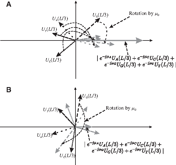
Aligning the four vectors according to the spectral rotation technique. Rotation and alignment of the vectors arg[UA(L/3)], arg[U_C(L/3)], arg[U_G(L/3)] and arg[U_T(L/3)] by μ_A, μ_C, μ_G and μ_T, respectively. (A) In coding regions. (B) In non-coding regions.

Kotlar and Lavner (2003) also proposed a G rotation (GR) measure for detecting short exons. The measure uses one statistical parameter that has a narrow distribution in short sequences. They selected arg[U_G(L/3)] since it has a narrow distribution when short exons with lengths of 120 bp are analyzed. In order to discriminate between coding and non-coding regions, the measure sums the vector U_G(L/3) rotated by μ_G with a reference value, |U_G(L/3)|. When U_G(L/3) belongs to a coding region and is rotated clockwise by μ_G, it will be directed towards the positive real axis. Therefore, adding |U_G(L/3)| to it will increase the magnitude. On the other hand, when U_G(L/3) belongs to a non-coding region, rotating it clockwise by μ_G will direct it to any direction. Therefore, summing it with the vector |U_G(L/3)| will decrease the magnitude of the resultant vector. Figure 3 shows a diagram that explains the process. Using |U_G(L/3)| as a reference vector provides discrimination between coding and non-coding regions. The GR measure is formulated as follows: \documentclass{aastex}\usepackage{amsbsy}\usepackage{amsfonts}\usepackage{amssymb}\usepackage{bm}\usepackage{mathrsfs}\usepackage{pifont}\usepackage{stmaryrd}\usepackage{textcomp}\usepackage{portland,xspace}\usepackage{amsmath,amsxtra}\pagestyle{empty}\DeclareMathSizes{10}{9}{7}{6} \begin{document} \begin{align*} \mid V_G \mid ^2 = \left|e^{- j \tilde{\mu}_G}U_G (L / 3) + \mid U_G (L / 3) \mid \right|^2 \tag{10} \end{align*} \end{document}

FIG. 3.

Aligning the U_G(L/3) vector according to the G rotation measure. Rotation and alignment of the vector U_G(L/3) by μ_G, and summing it with the reference ∣U_G(L/3)∣. (A) arg[U_G(L/3)] ≈ μ_G. (B) arg[U_G(L/3)] is any random value.

The technique uses a sliding window in the analysis. It is data-driven since statistical parameters are used in the analysis. Our analysis of the computational complexity of this technique shows that it is O(N), where N is the length of the sequence. The window length is the only parameter that has to be set (Kotlar and Lavner, 2003).

2.4. Exon prediction by nucleotide distribution

Digital signal processing-based gene finding algorithms use a fixed length window of a DNA signal in analyzing the spectrum properties of DNA sequences. A small window length emphasizes the small peaks that appear due to background noise; in addition, a large window length causes short exons or introns in DNA sequences to be missed (Tiwari et al., 1997; Liew et al., 2005). The 3-base periodicity in DNA sequences is caused by the unbalanced distributions of the four nucleotides in the three reading frames (codon positions). It has been observed that in exonic regions the nucleotide distributions in the three reading frames are unbalanced; however, these distributions are balanced in intronic regions. The unbalanced distribution in the three exonic reading frames occurs because there is redundant mapping in coding amino acids, and proteins prefer specific amino acid compositions (Fickett, 1982).

Yin and Yau (2005, 2007) studied the relationship between the 3-base periodicity and the nucleotide distributions by calculating the nucleotide frequencies at the three reading frames: \documentclass{aastex}\usepackage{amsbsy}\usepackage{amsfonts}\usepackage{amssymb}\usepackage{bm}\usepackage{mathrsfs}\usepackage{pifont}\usepackage{stmaryrd}\usepackage{textcomp}\usepackage{portland,xspace}\usepackage{amsmath,amsxtra}\pagestyle{empty}\DeclareMathSizes{10}{9}{7}{6} \begin{document} \begin{align*} \left[\begin{matrix} F_{A1} & F_{A2} & F_{A3} \\ F_{C1} & F_{C2} & F_{C3} \\ F_{G1} & F_{G2} & F_{G3} \\ F_{T1} & F_{T2} & F_{T3} \end{matrix} \right]\tag{11} \end{align*} \end{document}

where F_xi is the frequency of the nucleotide x at the reading frame i and \documentclass{aastex}\usepackage{amsbsy}\usepackage{amsfonts}\usepackage{amssymb}\usepackage{bm}\usepackage{mathrsfs}\usepackage{pifont}\usepackage{stmaryrd}\usepackage{textcomp}\usepackage{portland,xspace}\usepackage{amsmath,amsxtra}\pagestyle{empty}\DeclareMathSizes{10}{9}{7}{6}\begin{document}$$x \in \{A, C, G, T \} $$\end{document} . They concluded that the 3-base periodicity of a nucleotide is strong if the distribution of the nucleotide among the three reading frames is unbalanced. They proposed that the power spectrum at frequency 1/3 of a DNA sequence depends on the variance of nucleotide distributions in the three reading frames, where N is the length of the DNA sequence. They found that the variance of the nucleotide distributions in the three reading frames contributes to the 3-base periodicity in DNA sequences. This variance can be computed as follows: \documentclass{aastex}\usepackage{amsbsy}\usepackage{amsfonts}\usepackage{amssymb}\usepackage{bm}\usepackage{mathrsfs}\usepackage{pifont}\usepackage{stmaryrd}\usepackage{textcomp}\usepackage{portland,xspace}\usepackage{amsmath,amsxtra}\pagestyle{empty}\DeclareMathSizes{10}{9}{7}{6} \begin{document} \begin{align*} \sigma_ {x} = \sum_ {i = 1, 2, 3} \left(F_ {xi} - \frac {1} {3 } \sum_ {j = 1, 2, 3} F_ {xj} \right) ^2, \qquad x \in \{A, C, G, T \} \tag {12} \end{align*} \end{document}

The total measurement of the imbalance in the nucleotide distributions in the three reading frames can be computed as the sum of the variances of the nucleotides as follows: \documentclass{aastex}\usepackage{amsbsy}\usepackage{amsfonts}\usepackage{amssymb}\usepackage{bm}\usepackage{mathrsfs}\usepackage{pifont}\usepackage{stmaryrd}\usepackage{textcomp}\usepackage{portland,xspace}\usepackage{amsmath,amsxtra}\pagestyle{empty}\DeclareMathSizes{10}{9}{7}{6} \begin{document} \begin{align*} F_3 = \sum_{x = A, C, G, T} \sigma_x \tag{13} \end{align*} \end{document}

From formulas (12) and (13), we can get: \documentclass{aastex}\usepackage{amsbsy}\usepackage{amsfonts}\usepackage{amssymb}\usepackage{bm}\usepackage{mathrsfs}\usepackage{pifont}\usepackage{stmaryrd}\usepackage{textcomp}\usepackage{portland,xspace}\usepackage{amsmath,amsxtra}\pagestyle{empty}\DeclareMathSizes{10}{9}{7}{6} \begin{document} \begin{align*} F_3 = \frac {2} {3} \sum_ {x = A, C, G, T} \bigg (F^2_ {x1} + F^2_ {x2} + F^2_ {x3} - \left(F_ {x1} \times F_ {x2} + F_ {x2} \times F_ {x3} + F_ {x1} \times F_ {x3} \right) \bigg) \tag {14} \end{align*} \end{document}

To investigate the relationship between the frequency variance of the three reading frames and the value of the spectrum at frequency N/3, (PS(N/3)), Yin and Yau (2005) plotted the PS(N/3) that was computed by the DFT versus the corresponding variance frequency F₃. Their results showed that there is a linear relationship between PS(N/3) and F₃. The slope of this linear relationship was 3:2. PS(N/3) is computed by the DFT as follows: \documentclass{aastex}\usepackage{amsbsy}\usepackage{amsfonts}\usepackage{amssymb}\usepackage{bm}\usepackage{mathrsfs}\usepackage{pifont}\usepackage{stmaryrd}\usepackage{textcomp}\usepackage{portland,xspace}\usepackage{amsmath,amsxtra}\pagestyle{empty}\DeclareMathSizes{10}{9}{7}{6} \begin{document} \begin{align*} PS (N / 3) = \sum_{x = A, C, G, T} \left|\sum_{n = 0}^{N - 1}f_x (n) e^{- j2 \pi n / 3} \right|^2 \tag{15} \end{align*} \end{document}

where f_x(n) is the binary indicator sequence of nucleotide x, which was proposed by Voss (1992), and N is the length of the sequence. Therefore, it was suggested that PS(N/3) can be computed by formula (16) without computing the DFT of a DNA sequence. The computation time of this method is much less than the DFT method. For a window of length L, the computational complexity of the DFT method is O(NL); however, in the proposed method, the computational complexity is O(N). Moreover, the computation is accumulative since about 95% of the computation of the window is reused in the following slid window and this decreases the processing time. \documentclass{aastex}\usepackage{amsbsy}\usepackage{amsfonts}\usepackage{amssymb}\usepackage{bm}\usepackage{mathrsfs}\usepackage{pifont}\usepackage{stmaryrd}\usepackage{textcomp}\usepackage{portland,xspace}\usepackage{amsmath,amsxtra}\pagestyle{empty}\DeclareMathSizes{10}{9}{7}{6} \begin{document} \begin{align*} PS (N / 3) = \frac {3} {2} F_3 \tag {16}\end{align*} \end{document}

They concluded that the background noise of a DNA sequence of length N is related to the average power spectrum of the sequence. The ratio of the 3-base periodicity signal to the background noise of a DNA sequence is computed as follows: \documentclass{aastex}\usepackage{amsbsy}\usepackage{amsfonts}\usepackage{amssymb}\usepackage{bm}\usepackage{mathrsfs}\usepackage{pifont}\usepackage{stmaryrd}\usepackage{textcomp}\usepackage{portland,xspace}\usepackage{amsmath,amsxtra}\pagestyle{empty}\DeclareMathSizes{10}{9}{7}{6} \begin{document} \begin{align*} SNR (N) = \frac {PS (N / 3)} {N} \tag {17} \end{align*} \end{document}

SNR(N) can be considered as the strength of the 3-base periodicity per nucleotide. The experimental results, which included simulations on genomic sequences from Yeast and C. elegans (eukaryotes), have shown that SNR(N) is larger than or equal to 2 for most exonic sequences, while it is less than 2 for most intronic sequences. This property has been utilized by Yin and Yau (2007) in developing a new technique for predicting coding regions in DNA sequences. This technique is called exon prediction by nucleotide distribution (EPND). In this technique, there is no need to determine a window length since the sequence is processed accumulatively. As was mentioned above, the technique does not use the DFT.

For a DNA sequence of length N, let U_k denote the DNA walk sequence of length k. U_k is a sub-sequence of the DNA sequence ranging from the beginning to the position k. The EPND technique is summarized in Algorithm 2.

Algorithm 2

The Algorithm of the coding region predictor based on nucleotide distribution

1.	Set k = 1.
2.	Compute the nucleotide distributions of U_k in the three reading frames of F_xi where \documentclass{aastex}\usepackage{amsbsy}\usepackage{amsfonts}\usepackage{amssymb}\usepackage{bm}\usepackage{mathrsfs}\usepackage{pifont}\usepackage{stmaryrd}\usepackage{textcomp}\usepackage{portland,xspace}\usepackage{amsmath,amsxtra}\pagestyle{empty}\DeclareMathSizes{10}{9}{7}{6}\begin{document}$$x \in \{A, C, G, T \} $$\end{document} and \documentclass{aastex}\usepackage{amsbsy}\usepackage{amsfonts}\usepackage{amssymb}\usepackage{bm}\usepackage{mathrsfs}\usepackage{pifont}\usepackage{stmaryrd}\usepackage{textcomp}\usepackage{portland,xspace}\usepackage{amsmath,amsxtra}\pagestyle{empty}\DeclareMathSizes{10}{9}{7}{6}\begin{document}$$i \in \{1, 2, 3 \} $$\end{document} .
3.	Compute the magnitude of the 3-base periodicity PS(k/3) in U_k based on the formula (16) as follows:
	\documentclass{aastex}\usepackage{amsbsy}\usepackage{amsfonts}\usepackage{amssymb}\usepackage{bm}\usepackage{mathrsfs}\usepackage{pifont}\usepackage{stmaryrd}\usepackage{textcomp}\usepackage{portland,xspace}\usepackage{amsmath,amsxtra}\pagestyle{empty}\DeclareMathSizes{10}{9}{7}{6} \begin{document} \begin{align} PS (k / 3) = \frac {3} {2} F_3 \tag {18} \end{align} \end{document}
4.	Compute the signal-to-noise ratio SNR(k) for the sequence U_k by formula (17).
5.	Increase k by 1 and repeat steps 2-4 until k = N.
6.	Compute the slope of SNR at each position as follows:
	\documentclass{aastex}\usepackage{amsbsy}\usepackage{amsfonts}\usepackage{amssymb}\usepackage{bm}\usepackage{mathrsfs}\usepackage{pifont}\usepackage{stmaryrd}\usepackage{textcomp}\usepackage{portland,xspace}\usepackage{amsmath,amsxtra}\pagestyle{empty}\DeclareMathSizes{10}{9}{7}{6} \begin{document} \begin{align} SL (i) = \frac {SNR (i) - SNR (i - 50)} {50}, \qquad i = 51, 52 , \cdots N \tag {19} \end{align} \end{document}
	The slope is computed over 50 bp since the authors claim that the minimum length of exons and introns is not less than 50 bp (Yin and Yau, 2007). However, the histograms of the distribution of the lengths of exons in eukaryotes show that there are exons with lengths less than 50 bp but with low percentage (Long et al., 1995; Deutsch and Long, 1999).
7.	If the slope at the position i is larger than 0 and SNR(i) is greater than or equal to 2, set the nucleotide at this position as an exon nucleotide; otherwise, set the nucleotide as an intron nucleotide.
8.	Eliminate false positives and false negatives: if an exon region is less than 50 bp and flanked by two introns, this region is set as an intron region. In addition, if an intron region is less than 50 bp and flanked by two exons, this region is set to an exon region.

Yin and Yau (2007) stated that the algorithm does not work well with long DNA sequences which contain multiple exons and introns because the accumulated signal-to-noise ratio of the last exon will be low, especially when the exon comes after a long intron since the low SNR of the long intron dominates the high SNR of the following short exon. This affects the prediction accuracy. Therefore, the algorithm has been improved by dividing the long sequences into different subsequences (Yin and Yau, 2007). The improvement is summarized in Algorithm 3.

Algorithm 3

The improved EPND algorithm

1.	The DNA sequence is divided into subsequences of 2000 bp if it is longer than 2000 bp.
2.	Divide each subsequence into six even-spaced points:P₁ = 1, P₂ = 401, P₃ = 801, P₄ = 1201, P₅ = 1601 and P₆ = 2000.
3.	Identify exon or intron nucleotides using the EPND method on the subsequence between points P_i and P₆, where i = 1, 2, 3, 4, 5. Some of the nucleotides will be tested more than one time. A nucleotide is identified as an exon nucleotide when it is predicted as an exon region in the majority of the tests.

The advantage of this technique is that it does not need to determine a window length as in other DFT-based methods. The disadvantage of using a sliding window is that a window length parameter should be determined, which means the accuracy of the results will be dependent on the choice of this parameter since the optimum value of the window length is close to the lengths of the exons to be predicted (Liew et al., 2005). Using a short window will emphasize the statistical oscillations in non-coding regions, and this will increase the false positive exons. In addition, when a long window is used, short exons or introns will be missed. Therefore, the window length parameter is avoided in this technique. Compared with other DFT-based methods, the technique does not compute the DFT for the sequence. In addition, computing the frequencies of the nucleotides in the three reading frames can be done accumulatively. The method is not data-driven since no training data or statistical information is required in this technique. The authors state that the computational complexity of the technique is O(N), which is much less than the complexity of DFT-based methods.

The shortcoming of the technique is that the threshold is determined experimentally, and it might not work with different datasets. In genomes with long introns and short exons, the threshold might not work because the signal-to-noise ratio will be low, and there will be false negatives. In addition, segmenting the sequence into subsequences and computing the signal-to-noise ratio for each subsequence individually might cause a prediction error when there is an exon spanning the point of segmentation.

2.5. Optimized gene predictor

Jiang et al. (2008) proposed a gene prediction technique based on a 2D graphical representation method. This representation method does not cause degeneracy, i.e., there is a one-to-one correspondence between the universal representation graph and the original DNA sequence. When a representation method causes degeneration, biological information is lost, and the original DNA sequence cannot be recovered from its representation graph.

The graphical representation method uses a two-quadrant Cartesian coordinate system for representing DNA sequences. The four nucleotides are represented by four independent vectors as follows: \documentclass{aastex}\usepackage{amsbsy}\usepackage{amsfonts}\usepackage{amssymb}\usepackage{bm}\usepackage{mathrsfs}\usepackage{pifont}\usepackage{stmaryrd}\usepackage{textcomp}\usepackage{portland,xspace}\usepackage{amsmath,amsxtra}\pagestyle{empty}\DeclareMathSizes{10}{9}{7}{6} \begin{document} \begin{align*} &(\sin \theta, - \cos \theta) \rightarrow A \\ &(\cos \theta, \sin \theta) \rightarrow C \\ &(\cos \theta, - \sin \theta) \rightarrow G \\ &(\sin \theta, \cos \theta) \rightarrow T \tag{20} \end{align*} \end{document}

where \documentclass{aastex}\usepackage{amsbsy}\usepackage{amsfonts}\usepackage{amssymb}\usepackage{bm}\usepackage{mathrsfs}\usepackage{pifont}\usepackage{stmaryrd}\usepackage{textcomp}\usepackage{portland,xspace}\usepackage{amsmath,amsxtra}\pagestyle{empty}\DeclareMathSizes{10}{9}{7}{6}\begin{document}$$0 < \theta < \frac {\pi} {2} $$\end{document} and \documentclass{aastex}\usepackage{amsbsy}\usepackage{amsfonts}\usepackage{amssymb}\usepackage{bm}\usepackage{mathrsfs}\usepackage{pifont}\usepackage{stmaryrd}\usepackage{textcomp}\usepackage{portland,xspace}\usepackage{amsmath,amsxtra}\pagestyle{empty}\DeclareMathSizes{10}{9}{7}{6}\begin{document}$$\theta \neq \frac {\pi} {4} $$\end{document} . The graphical representation of the four nucleotides is shown in Figure 4. Each nucleotide is represented as a unit vector.

FIG. 4.

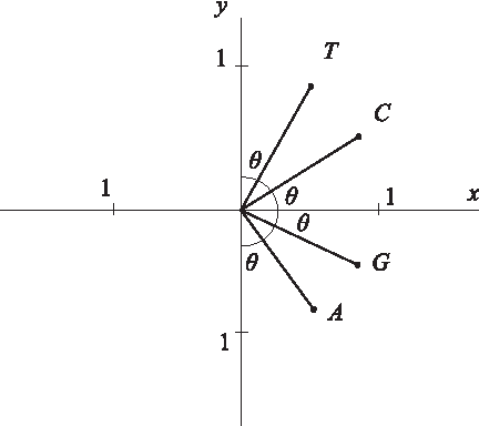
The unit vectors of the graphical representation in the Cartesian coordinate plane.

The amplitude characteristic of this representation method reflects the distribution of the four nucleotides along the DNA sequence. The amplitude at each point in the representation graph represents the sum of the amplitudes of the preceding points. Therefore, a change in the amplitude can reflect a change in the distribution of the four nucleotides along the DNA sequence (Jiang et al., 2008).

Let \documentclass{aastex}\usepackage{amsbsy}\usepackage{amsfonts}\usepackage{amssymb}\usepackage{bm}\usepackage{mathrsfs}\usepackage{pifont}\usepackage{stmaryrd}\usepackage{textcomp}\usepackage{portland,xspace}\usepackage{amsmath,amsxtra}\pagestyle{empty}\DeclareMathSizes{10}{9}{7}{6}\begin{document}$$S = \{a_1, a_2, a_3, \ldots, a_N \} $$\end{document} be a DNA sequence. S can be mapped to the representation graph by representing the four nucleotide sequences as follows: \documentclass{aastex}\usepackage{amsbsy}\usepackage{amsfonts}\usepackage{amssymb}\usepackage{bm}\usepackage{mathrsfs}\usepackage{pifont}\usepackage{stmaryrd}\usepackage{textcomp}\usepackage{portland,xspace}\usepackage{amsmath,amsxtra}\pagestyle{empty}\DeclareMathSizes{10}{9}{7}{6} \begin{document} \begin{align*} S_a [ k ] = \begin{cases} \sin \theta - j \cos \theta, \quad a_k = A \\ 0 \qquad \qquad \quad, \quad a_k \neq A\end{cases} \\ S_c [ k ] = \begin{cases} \cos \theta + j \sin \theta, \quad a_k= C \\ 0 \qquad \qquad \quad, \quad a_k \neq C\end{cases}\\ S_g [ k ] = \begin{cases} \cos \theta - j \sin \theta, \quad a_k = G \\ 0 \qquad \qquad \quad, \quad a_k \neq G\end{cases}\\ S_t [ k ] = \begin{cases} \sin \theta + j \cos \theta, \quad a_k = T \\ 0 \qquad \qquad \quad, \quad a_k \neq T\end{cases}\tag{21} \end{align*} \end{document}

where S_a[k], S_c[k], S_g[k], and S_t[k] are respectively the sequences of the nucleotides A, C, G, and T represented in the graphical representation and k is the base pair position. The DFT is applied to each of the four sequences to get four spectral representations S_A(k), S_C(k), S_G(k), and S_T(k). The upper case subscript is to show that the sequences are in the frequency domain. The power spectrum of a DNA sequence is computed as follows: \documentclass{aastex}\usepackage{amsbsy}\usepackage{amsfonts}\usepackage{amssymb}\usepackage{bm}\usepackage{mathrsfs}\usepackage{pifont}\usepackage{stmaryrd}\usepackage{textcomp}\usepackage{portland,xspace}\usepackage{amsmath,amsxtra}\pagestyle{empty}\DeclareMathSizes{10}{9}{7}{6} \begin{document} \begin{align*} S (k) = \mid S_A (k) \mid^2 + \mid S_C (k) \mid^2 + \mid S_G (k) \mid^2 + \mid S_T (k) \mid^2 \tag{22} \end{align*} \end{document}

Based on the above representation graph, the proposed gene prediction technique suggests a simple coding region predictor W(j, L), which determines whether the nucleotide at position j is a coding region or not, where L is the window length. The predictor is given as follows: \documentclass{aastex}\usepackage{amsbsy}\usepackage{amsfonts}\usepackage{amssymb}\usepackage{bm}\usepackage{mathrsfs}\usepackage{pifont}\usepackage{stmaryrd}\usepackage{textcomp}\usepackage{portland,xspace}\usepackage{amsmath,amsxtra}\pagestyle{empty}\DeclareMathSizes{10}{9}{7}{6} \begin{document} \begin{align*} W (j, L) = \mid a \mid A_L \mid ^2 + c \mid C_L \mid ^2 + g \mid G_L \mid ^2 + t \mid T_L \mid ^2 \mid \tag{23} \end{align*} \end{document}

where parameters a, c, g, and t represent the complex values: \documentclass{aastex}\usepackage{amsbsy}\usepackage{amsfonts}\usepackage{amssymb}\usepackage{bm}\usepackage{mathrsfs}\usepackage{pifont}\usepackage{stmaryrd}\usepackage{textcomp}\usepackage{portland,xspace}\usepackage{amsmath,amsxtra}\pagestyle{empty}\DeclareMathSizes{10}{9}{7}{6} \begin{document} \begin{align*} a =\sin \theta - j \cos \theta \\ c = \cos \theta + j \sin \theta\\ g = \cos \theta - j \sin \theta\\ t = \sin \theta + j \cos \theta \tag{24} \end{align*} \end{document}

and \documentclass{aastex}\usepackage{amsbsy}\usepackage{amsfonts}\usepackage{amssymb}\usepackage{bm}\usepackage{mathrsfs}\usepackage{pifont}\usepackage{stmaryrd}\usepackage{textcomp}\usepackage{portland,xspace}\usepackage{amsmath,amsxtra}\pagestyle{empty}\DeclareMathSizes{10}{9}{7}{6} \begin{document} \begin{align*} A_L = \frac {1} {L} S_A (L / 3) _j \\ C_L = \frac {1} {L} S_C (L / 3) _j \\ G_L = \frac {1} {L} S_G (L / 3) _j \\ T_L = \frac {1} {L} S_T (L / 3) _j \tag {25} \end{align*} \end{document}

where S_A(L/3)_j, S_C(L/3)_j, S_G(L/3)_j, and S_T(L/3)_j are DFT coefficients at frequency k = L/3 for a subsequence with a window width L starting at nucleotide j. The technique of coding region prediction based on the W(j, L) predictor is summarized in Algorithm 4.

Algorithm 4

The Algorithm of the coding region predictor using the universal representation method

1.	Select an arbitrary window length L, and set j to 1.
2.	Compute W(j, L) for the current value of j by formula (23).
3.	The mean over the entire window is computed to get the smoothed version W_s(j, L) of W(j, L).
4.	Increase j by 1.
5.	If j is less than or equal to N − L, repeat steps 2–4, where N is the length of the DNA sequence.
6.	The mean W_sm(L) of the whole W_s(j, L) is computed and used as a threshold.
7.	For j = 1 to N, If the nucleotide at position j in W_s(j, L) is above the threshold, it is considered as an exon region; otherwise, it is considered as an intron region.
8.	Compute the modified window length L_m based on the lengths of the predicted exons. The value of L_m is computed as the average of the lengths of the predicted exons as follows:
	\documentclass{aastex}\usepackage{amsbsy}\usepackage{amsfonts}\usepackage{amssymb}\usepackage{bm}\usepackage{mathrsfs}\usepackage{pifont}\usepackage{stmaryrd}\usepackage{textcomp}\usepackage{portland,xspace}\usepackage{amsmath,amsxtra}\pagestyle{empty}\DeclareMathSizes{10}{9}{7}{6} \begin{document} \begin{align} L_m = \frac {\sum\limits_ {d = 1}^{n} L_d} {n} \tag {26 } \end{align} \end{document}
	where n is the number of the predicted exons, L_d is the length of the predicted exon d.
9.	Set L = L_m and j = 1.
10.	Repeat steps 2–7 to predict the exons another time based on the new value of the window length.

The technique uses a sliding window in the analysis of DNA sequences. An arbitrary window length is used in the technique, and then a modified window length is computed based on the prediction done by the arbitrary window length. Adjusting the window length based on the lengths of the predicted exons will make it close to the lengths of the exons. This improves the prediction accuracy when it is repeated based on the modified window length since the window length will be greater than or equal to the minimum length of the exons. When the window length is close to the lengths of the exons to be predicted, the background 1/f noise is suppressed.

An optimized predictor P(L) has been proposed based on the predictor W(j, L). The predictor P(L) is the mean of all ratios between the value of \documentclass{aastex}\usepackage{amsbsy}\usepackage{amsfonts}\usepackage{amssymb}\usepackage{bm}\usepackage{mathrsfs}\usepackage{pifont}\usepackage{stmaryrd}\usepackage{textcomp}\usepackage{portland,xspace}\usepackage{amsmath,amsxtra}\pagestyle{empty}\DeclareMathSizes{10}{9}{7}{6}\begin{document}$$W (j + \lfloor {L}/ {3} \rfloor + 1, L)$$\end{document} , where j is the position offset from the start of the sequence, and the window size L: \documentclass{aastex}\usepackage{amsbsy}\usepackage{amsfonts}\usepackage{amssymb}\usepackage{bm}\usepackage{mathrsfs}\usepackage{pifont}\usepackage{stmaryrd}\usepackage{textcomp}\usepackage{portland,xspace}\usepackage{amsmath,amsxtra}\pagestyle{empty}\DeclareMathSizes{10}{9}{7}{6} \begin{document} \begin{align*} P (L) = \frac {\sum\limits_ {j = 1} ^ {N - L} \frac {W (j + \lfloor \frac {L} {3} \rfloor + 1, L)} {L}} {N - L} \tag {27} \end{align*} \end{document}

The predictor W(j, L) is first used to predict exons and introns and their corresponding boundaries. Then the P(L) value is calculated for each exon and intron. If the value of P(L) is greater than or equal to 1, the region is recognized as an exon; otherwise, it is recognized as an intron. Therefore, the predictor P(L) will either confirm the prediction of exons and introns which are already predicted by W(j, L) or readjust the prediction done by W(j, L). The P(L) predictor can disprove the prediction of small noise peaks that exceed the threshold in the W(j, L) predictor.

We have proposed an equivalent, but simpler, formula to compute P(L). This formula computes P(L) for each region predicted by W(j, L). The formula computes P(L) as the mean of the ratios of W(j, L) to the window length L for each coding region as follows: \documentclass{aastex}\usepackage{amsbsy}\usepackage{amsfonts}\usepackage{amssymb}\usepackage{bm}\usepackage{mathrsfs}\usepackage{pifont}\usepackage{stmaryrd}\usepackage{textcomp}\usepackage{portland,xspace}\usepackage{amsmath,amsxtra}\pagestyle{empty}\DeclareMathSizes{10}{9}{7}{6} \begin{document} \begin{align*} P (L) _m = \frac {\sum\limits_ {j = LB_m} ^ {UB_m} \frac {W (j, L)} {L}} {K_m} \tag {28} \end{align*} \end{document}

where LB_m and UB_m are respectively the lower and upper bounds of the m^th predicted region(exon or intron), K_m is its length and P(L)_m is the value of P(L) for the m^th region. Furthermore, A_L, C_L, G_L and T_L could be computed as follows: \documentclass{aastex}\usepackage{amsbsy}\usepackage{amsfonts}\usepackage{amssymb}\usepackage{bm}\usepackage{mathrsfs}\usepackage{pifont}\usepackage{stmaryrd}\usepackage{textcomp}\usepackage{portland,xspace}\usepackage{amsmath,amsxtra}\pagestyle{empty}\DeclareMathSizes{10}{9}{7}{6} \begin{document} \begin{align*} A_L = S_A (L / 3) _j \\ C_L = S_C (L / 3) _j \\ G_L = S_G (L / 3) _j \\ T_L = S_T (L / 3) _j \tag{29} \end{align*} \end{document}

According to formula (29), the values of W(j, L) could be greater than 1; as a result, the value of P(L) can be greater than or equal to 1 for exons. According to a personal correspondence with the first author, he has confirmed formulas (28) and (29).

The advantage of this technique is that the threshold is computed based on the DNA sequence to be predicted, and it is not determined based on experimental or training data, which might not be available. Therefore, the threshold is computed intrinsically, and it is specific to the sequence itself. In addition, the technique is not data-driven since it does not use any training data or statistical information in the analysis or the computation of the threshold as has been mentioned. The advantage of this method is that it can be used to analyze genomic data of species for which there is no previous knowledge available. Therefore, these methods can be used to annotate novel genomic sequences (Mena-Chalco et al., 2008).

We can identify the computational complexity of this technique to be O(NL), where N is the length of the DNA sequence, and L is the window length. The angle θ, used in the four representation vectors of the nucleotides, is a parameter that should be determined since the complex parameters a, c, g and t given in formula (24), which depend on θ, weight the power spectra A_L, C_L, G_L and T_L respectively as shown in formula (23). Anastassiou (2000) optimized complex parameters to obtain maximum differentiation between coding regions and non-coding regions, and used them in a formula similar to formula (23). Therefore, the optimum value of this angle might be different from sequence to sequence. Although an adjusted window length is computed, the initial window length L is another parameter that should be set.

2.6. Time-frequency domain method

Akhtar et al. (2008b) proposed a time-frequency domain method (TFDM) for gene prediction in eukaryotes. The method combines time-domain and frequency-domain measures. They demonstrated some DSP-based features for gene prediction. The DSP-based features have included spectral and statistical properties of DNA sequences. The paired numerical representation has been used for mapping DNA sequences. The paired representation depends on the property of the frequency of distribution of nucleotides A − T, and C − G. This property is based on the fact that intron regions are rich in nucleotides A and T, while exon regions are rich in nucleotides C and G. DNA sequences are converted into two binary indicator sequences x_A_− T[n] and x_C_− G[n]. This representation incorporates a useful structural property and reduces the computational cost (Akhtar et al., 2008a,b). However, we denote that this representation scheme causes degeneracy, and the original DNA sequence cannot be retrieved from the mapping since there is no one-to-one correspondence between the original sequence and its representation.

One of the measures that Akhtar et al. (2008a) proposed is the paired and weighted spectral rotation measure (PWSR). This measure uses the paired representation to extract the statistical and spectral properties that differentiate coding regions from non-coding regions in DNA sequences. The DFT is the analysis tool that is used to compute the period-3 spectrum. A sliding window with a specific length L is used in the analysis of DNA sequences. The model is data-driven since it uses training data to compute the means μ_m and the standard deviations σ_m of the distributions of the DFT phase angles of coding regions. In other words, the average of the DFT phase angles over each coding region is computed, and then μ_m and σ_m of these averages are computed. In addition, the frequencies of occurrences of nucleotides “A or T” and “C or G” in coding regions are used as weights w_m and calculated from the training data, where \documentclass{aastex}\usepackage{amsbsy}\usepackage{amsfonts}\usepackage{amssymb}\usepackage{bm}\usepackage{mathrsfs}\usepackage{pifont}\usepackage{stmaryrd}\usepackage{textcomp}\usepackage{portland,xspace}\usepackage{amsmath,amsxtra}\pagestyle{empty}\DeclareMathSizes{10}{9}{7}{6}\begin{document}$$m \in \{A - T, C - G \} $$\end{document} . The period-3 feature is extracted using the following formula: \documentclass{aastex}\usepackage{amsbsy}\usepackage{amsfonts}\usepackage{amssymb}\usepackage{bm}\usepackage{mathrsfs}\usepackage{pifont}\usepackage{stmaryrd}\usepackage{textcomp}\usepackage{portland,xspace}\usepackage{amsmath,amsxtra}\pagestyle{empty}\DeclareMathSizes{10}{9}{7}{6} \begin{document} \begin{align*} {PWSR_l} [k ] = \left|\frac {e^ {- j \mu_ {A - T}}} {\sigma_ {A - T}} \cdot w_ {A - T} \cdot X_ {A - T} [ k ] + \frac {e^ {- j \mu_ {C - G}}} {\sigma_ {C - G}} \cdot w_ {C - G} \cdot X_ {C - G } [ k ] \right| ^2 \tag {30} \end{align*} \end{document}

where k = L/3 and l denotes the forward (F) and reverse (R) directions of a DNA sequence since PWSR_l[k] is computed for the forward and the reverse directions of a DNA sequence and these are combined as follows: \documentclass{aastex}\usepackage{amsbsy}\usepackage{amsfonts}\usepackage{amssymb}\usepackage{bm}\usepackage{mathrsfs}\usepackage{pifont}\usepackage{stmaryrd}\usepackage{textcomp}\usepackage{portland,xspace}\usepackage{amsmath,amsxtra}\pagestyle{empty}\DeclareMathSizes{10}{9}{7}{6} \begin{document} \begin{align*} {PWSR} [k] = {PWSR_F} [k] + {PWSR_R} [k] \tag{31} \end{align*} \end{document}

The problem with this measure is it requires training from genomic sequences of a related organism, and these sequences might not be available.

Akhtar et al. (2008a) proposed another frequency-domain measure which is the paired spectral content (PSC) measure. This measure does not need training data from the same organism. The DNA sequence is converted to a single numerical sequence using the paired-numerical representation. Nucleotides A and T are denoted by +1, and nucleotides C and G are denoted by −1. Then the measure combines the forward and backward DFTs of the same DNA sequence as follows: \documentclass{aastex}\usepackage{amsbsy}\usepackage{amsfonts}\usepackage{amssymb}\usepackage{bm}\usepackage{mathrsfs}\usepackage{pifont}\usepackage{stmaryrd}\usepackage{textcomp}\usepackage{portland,xspace}\usepackage{amsmath,amsxtra}\pagestyle{empty}\DeclareMathSizes{10}{9}{7}{6} \begin{document} \begin{align*} {PSC} [ k ] = \mid X_F [ k ] \mid^2 + \mid X_R [ k ] \mid^2 \tag{32} \end{align*} \end{document}

where X_F[k] and X_R[k] are, respectively, the DFTs of the paired-numerical sequence x[n] in the forward and reverse directions. The PSC measure can be applied to sequences taken from any organism. There is not much difference between this measure and the traditional DFT method except the nucleotide representation scheme. A sliding window is used in the analysis of DNA sequences by this measure. Unlike the PWSR measure, the PSC measure is not data-driven since X_F[k] and X_R[k] are not weighted by statistical parameters. The authors state that involving the forward and reverse directions in the analysis increases the computational complexity. However, in terms of the representation method, they state that the computational complexity is reduced since two numerical sequences are processed instead of four (Akhtar et al., 2008a). We can identify the complexity of the two measures to be O(NL) for each direction, where N is the length of the DNA sequence, and L is the window length. The only parameter that has to be set is the window length L.

In the time-domain analysis, Akhtar et al. (2008a) proposed two algorithms that are the average magnitude difference function (AMDF) and the time domain periodogram (TDP). Pre-filtering for the four binary indicator sequences has been used in these algorithms. For this task, a second-order resonant filter centered at frequency 2π/3 has been used to extract the spectral component at this frequency and suppress or attenuate all other spectral components. A sliding window is used in the two measures to analyze the period-3 property. Since the two methods are time-domain, the DFT is not used here. The AMDF method is applied to the sequence x[n] as follows: \documentclass{aastex}\usepackage{amsbsy}\usepackage{amsfonts}\usepackage{amssymb}\usepackage{bm}\usepackage{mathrsfs}\usepackage{pifont}\usepackage{stmaryrd}\usepackage{textcomp}\usepackage{portland,xspace}\usepackage{amsmath,amsxtra}\pagestyle{empty}\DeclareMathSizes{10}{9}{7}{6} \begin{document} \begin{align*} {AMDF} [k ] = \frac {1} {L} \sum_ {n = 1} ^L \mid x [ n ] - x [ n - k ] \mid \tag {33} \end{align*} \end{document}

where L is the window length. k is set to 3 for period-3. A sliding window will move along the filtered sequence to compute AMDF[k] for the whole sequence, and the AMDFs of the four sequences are combined linearly.

According to the TDP method, the L-point window of data are arranged in a matrix with k columns and L/k rows; in other words, the first k samples of the sequence are arranged in the first row, the second k samples are arranged in the second row and so on, where k = 3 for period-3 testing (Akhtar et al., 2008a). Then the elements of the matrix are summed over the columns to obtain the TDP vector of size k as follows: \documentclass{aastex}\usepackage{amsbsy}\usepackage{amsfonts}\usepackage{amssymb}\usepackage{bm}\usepackage{mathrsfs}\usepackage{pifont}\usepackage{stmaryrd}\usepackage{textcomp}\usepackage{portland,xspace}\usepackage{amsmath,amsxtra}\pagestyle{empty}\DeclareMathSizes{10}{9}{7}{6} \begin{document} \begin{align*} {TDP}_{vector} [k ] = \left\{ \sum_{n = 1}^{L / k}x [ kn - (k - 1) ], \sum_{n = 1}^{L / k}x [ kn - (k - 2) ], \cdots \sum_{n = 1}^{L / k}x [ kn ] \right\} \tag{34} \end{align*} \end{document}

The estimate of the degree of periodicity is calculated as follows: \documentclass{aastex}\usepackage{amsbsy}\usepackage{amsfonts}\usepackage{amssymb}\usepackage{bm}\usepackage{mathrsfs}\usepackage{pifont}\usepackage{stmaryrd}\usepackage{textcomp}\usepackage{portland,xspace}\usepackage{amsmath,amsxtra}\pagestyle{empty}\DeclareMathSizes{10}{9}{7}{6} \begin{document} \begin{align*} {TDP} [ k ] = \max (TDP_{vector} [ k ]) - \min (TDP_{vector} [ k ] ) \tag{35} \end{align*} \end{document}

Considering that k equals 3, arranging the elements in the way mentioned above and then summing them is similar to finding the frequency of each nucleotide in the three reading frames. In addition, we denote calculating the degree of periodicity as shown in formula (35), this means finding the maximum bias of the nucleotide distributions in the three reading frames. This technique reminds us of the principle of the EPND (Yin and Yau, 2007) technique since the principles of the two techniques are somewhat related.

The AMDF and TDP techniques use a sliding window, and the choice of the window size could affect the results. Both of the AMDF and TDP techniques are not data-driven since no statistical or learning data is required in the processing. In the two techniques, we can determine the complexity of the filtering stage to be O(N) and the complexity of the extracting the period-3 spectrum using either of the two measures to be O(NL), where N is the length of the sequence. Some parameters could determine the accuracy of time-domain algorithms such as the power of the filter in removing the unfavorable spectral components. In addition, the choice of the window length might affect the results obtained from these methods.

In the TFDM, Akhtar et al. (2008b) combined the PWSR and AMDF measures to design a gene prediction algorithm. They modified the PWSR measure in formula (31) by using a suitable window shape and length. Signal boosting is performed on the output of the PWSR algorithm to enhance the spectrum signal and attenuate noise. The boosted signal is then combined with the output of the AMDF measure given in formula (33). A fusion method is used to combine the two outputs by normalizing the two outputs and combining them with unweighted sum.

2.7. Modified Gabor-Wavelet transform method

Mena-Chalco et al. (2008) proposed a technique based on a modified Gabor-wavelet transform (MGWT) to predict coding regions in DNA sequences. Using this transform, the method extracts the 3-base periodicity of DNA sequences. Then it will be possible to differentiate between coding and non-coding regions. The method does not use a sliding window, so it is not dependent on the window length parameter like other DFT-based methods. In this technique, the analysis is based on the wavelet transform.

The wavelet analysis of a signal u using the multiscale transform is defined as: \documentclass{aastex}\usepackage{amsbsy}\usepackage{amsfonts}\usepackage{amssymb}\usepackage{bm}\usepackage{mathrsfs}\usepackage{pifont}\usepackage{stmaryrd}\usepackage{textcomp}\usepackage{portland,xspace}\usepackage{amsmath,amsxtra}\pagestyle{empty}\DeclareMathSizes{10}{9}{7}{6} \begin{document} \begin{align*} U (b, a) = \int u (x) \psi (x, b, a) dx \tag{36} \end{align*} \end{document}

where a > 0 is the scale parameter, b is the time (or translation) parameter, and ψ is the analyzing function. The STFT and Gabor-wavelet transform functions are two possible analyzing functions that can be used in this problem. However, Mena-Chalco et al. (2008) showed that neither the STFT nor the Gabor-wavelet analyzing functions are suitable for the gene prediction problem. The STFT is also known as the Gabor transform and is defined as follows: \documentclass{aastex}\usepackage{amsbsy}\usepackage{amsfonts}\usepackage{amssymb}\usepackage{bm}\usepackage{mathrsfs}\usepackage{pifont}\usepackage{stmaryrd}\usepackage{textcomp}\usepackage{portland,xspace}\usepackage{amsmath,amsxtra}\pagestyle{empty}\DeclareMathSizes{10}{9}{7}{6} \begin{document} \begin{align*} \psi_ {STFT} (x, b, a) = e^ {- \frac {(x - b) ^2} {2}} e^ {j a (x - b)} \tag {37} \end{align*} \end{document}

The Gabor wavelet transform is defined as follows: \documentclass{aastex}\usepackage{amsbsy}\usepackage{amsfonts}\usepackage{amssymb}\usepackage{bm}\usepackage{mathrsfs}\usepackage{pifont}\usepackage{stmaryrd}\usepackage{textcomp}\usepackage{portland,xspace}\usepackage{amsmath,amsxtra}\pagestyle{empty}\DeclareMathSizes{10}{9}{7}{6} \begin{document} \begin{align*} \psi_ {GWT} (x, b, a) = e^ {- \frac {\left(\frac{x - b} {a}\right) ^2 } {2}} e^ {j \omega_0 \left(\frac {x - b} {a} \right)} \tag {38 } \end{align*} \end{document}

The two transforms analyze signals at different frequencies and scales, but the analysis is carried out in a dependent way, i.e., the frequency depends on the scale a. In other words, the scale cannot be changed while keeping the frequency constant. In formula (37), it can be noticed that varying the scale a causes a variation in the frequency, while the Gaussian standard deviation is kept constant. In formula (38), it is clear that varying the scale causes a variation in the frequency and Gaussian standard deviation. Both transforms are not suitable for analyzing DNA sequences since coding regions in DNA sequences are characterized by a specific periodicity which is 3-base periodicity which may occur at different scales. Therefore, the task here is to analyze these sequences at different scales while keeping the analysis frequency constant (Mena-Chalco et al., 2008). Mena-Chalco et al. (2008) modified formula (38) to keep the complex exponential frequency constant while varying the scale a. The modified Gabor wavelet transform is as follows: \documentclass{aastex}\usepackage{amsbsy}\usepackage{amsfonts}\usepackage{amssymb}\usepackage{bm}\usepackage{mathrsfs}\usepackage{pifont}\usepackage{stmaryrd}\usepackage{textcomp}\usepackage{portland,xspace}\usepackage{amsmath,amsxtra}\pagestyle{empty}\DeclareMathSizes{10}{9}{7}{6} \begin{document} \begin{align*} \psi_ {MGWT} (x, b, a) = e^ {- \frac {(x - b) ^2} {2a^2}} e^ {j \omega_0 (x - b)} \tag {39} \end{align*} \end{document}

Formula (39) is the analyzing function that Mena-Chalco et al. (2008) adopted in this technique. Algorithm 5 summarizes the steps of the MGWT technique.

Algorithm 5

Algorithm of the modified Gabor-wavelet transform

1.	Map the DNA sequence to four binary indicator sequences u_A, u_C, u_G, and u_T corresponding to the nucleotides A, C, G, and T, respectively.
2.	Apply the MGWT to each binary indicator sequence. The transforms are calculated for different scales and constant frequency ω₀. ω₀ is set to N/3 for 3-base periodicity analysis, where N is the length of the sequence. The transform of the four binary indicator sequences is given by:
	\documentclass{aastex}\usepackage{amsbsy}\usepackage{amsfonts}\usepackage{amssymb}\usepackage{bm}\usepackage{mathrsfs}\usepackage{pifont}\usepackage{stmaryrd}\usepackage{textcomp}\usepackage{portland,xspace}\usepackage{amsmath,amsxtra}\pagestyle{empty}\DeclareMathSizes{10}{9}{7}{6} \begin{document} \begin{align} U_ \alpha (b, a) = \int u_ \alpha (x) \psi_{MGWT} (x, b, a) dx \tag{40} \end{align} \end{document}
	where \documentclass{aastex}\usepackage{amsbsy}\usepackage{amsfonts}\usepackage{amssymb}\usepackage{bm}\usepackage{mathrsfs}\usepackage{pifont}\usepackage{stmaryrd}\usepackage{textcomp}\usepackage{portland,xspace}\usepackage{amsmath,amsxtra}\pagestyle{empty}\DeclareMathSizes{10}{9}{7}{6}\begin{document}$$\alpha \in \{A, C, G, T \} $$\end{document} , b is the position along the DNA sequence, and a is the scale parameter. The spectrum of each binary indicator sequence is calculated from its corresponding MGWT coefficients:
	\documentclass{aastex}\usepackage{amsbsy}\usepackage{amsfonts}\usepackage{amssymb}\usepackage{bm}\usepackage{mathrsfs}\usepackage{pifont}\usepackage{stmaryrd}\usepackage{textcomp}\usepackage{portland,xspace}\usepackage{amsmath,amsxtra}\pagestyle{empty}\DeclareMathSizes{10}{9}{7}{6} \begin{document} \begin{align} m_ \alpha (b, a) = \mid U_ \alpha (b, a) \mid^2 \tag{41} \end{align} \end{document}
	The spectrum of the DNA sequence is calculated by summing the spectra of the four binary sequences as follows:
	\documentclass{aastex}\usepackage{amsbsy}\usepackage{amsfonts}\usepackage{amssymb}\usepackage{bm}\usepackage{mathrsfs}\usepackage{pifont}\usepackage{stmaryrd}\usepackage{textcomp}\usepackage{portland,xspace}\usepackage{amsmath,amsxtra}\pagestyle{empty}\DeclareMathSizes{10}{9}{7}{6} \begin{document} \begin{align} M (b, a) = \sum_ \alpha m_ \alpha (b, a) \tag{42} \end{align} \end{document}
3.	Project the total spectrum onto the position axis to detect coding regions. Projection spectrum coefficients with strong 3-base periodicity will show high responses. For a sequence with length N, the projection of the spectrum onto the position axis is as follows:
	\documentclass{aastex}\usepackage{amsbsy}\usepackage{amsfonts}\usepackage{amssymb}\usepackage{bm}\usepackage{mathrsfs}\usepackage{pifont}\usepackage{stmaryrd}\usepackage{textcomp}\usepackage{portland,xspace}\usepackage{amsmath,amsxtra}\pagestyle{empty}\DeclareMathSizes{10}{9}{7}{6} \begin{document} \begin{align} M_p (b) = \sum_ \alpha M (b, a), \quad b = 0, 1, \cdots, N - 1 \tag{43} \end{align} \end{document}
4.	A threshold operation is applied to the projected spectrum to identify the coding regions. t percent small coefficients of M_p are set to zero, where t is a predetermined threshold. This percentage of small coefficients represents the non-coding regions coefficients.

The technique does not use a sliding window, so setting the window length parameter which affects the results is avoided. No training data is required, so the technique is not data-driven. The authors state that the complexity of the method is O(N log N), where N is the length of the biomolecular sequence. Two parameters have to be set, namely the scale range a and the threshold percentage t. The choice of these two parameters could affect the results and the optimum values could be different from one sequence to another.

2.8. An algorithm for gene prediction based on the Z curve

Based on the period-3 property of coding regions, Ma and Zhu (2007) proposed a technique that uses a kind of adaptive filter to predict the exons in DNA sequences. A recursive least squares (RLS) algorithm is used to predict the weights of the filter. The method adopts the Z curve representation as a numerical mapping of DNA sequences. The Z curve maps a DNA sequence to a three-dimensional curve. The sequence is mapped to three sequences—x₁(n), y₁(n), and z₁(n)—as follows: \documentclass{aastex}\usepackage{amsbsy}\usepackage{amsfonts}\usepackage{amssymb}\usepackage{bm}\usepackage{mathrsfs}\usepackage{pifont}\usepackage{stmaryrd}\usepackage{textcomp}\usepackage{portland,xspace}\usepackage{amsmath,amsxtra}\pagestyle{empty}\DeclareMathSizes{10}{9}{7}{6} \begin{document} \begin{align*} x_1 (n) = 2 [ x_A (n) + x_C (n) ] - 1 \\ y_1 (n) = 2 [ x_A (n) + x_G (n) ] - 1 \\ z_1 (n) = 2 [ x_A (n) + x_T (n) ] - 1 \tag{44} \end{align*} \end{document}

where x_A(n), x_C(n), x_G(n), and x_T(n) are the binary indicator sequences of the nucleotides A, C, G, and T at position n respectively. x₁(n), y₁(n), and z₁(n) will only have the values of 1 or −1. For each nucleotide, the three variables will have a distinct combination of the values of 1 and −1. Therefore, a DNA sequence can be decomposed into three sequences of digital signals, each with a clear biological meaning. The first sequence x₁ represents the distribution of the bases of purine/pyrimidine along the DNA sequence. The second sequence y₁ represents the distribution of the bases of the amino/keto types along the DNA sequence. The third sequence z₁ represents the distribution of the bases of the strong/weak hydrogen bonds along the sequence. Decomposing a DNA sequence into three sequences instead of four binary sequences reduces the computational cost (Ma and Zhu, 2007).

The adaptive filter is developed using the RLS algorithm which is a kind of adaptive algorithm. The principle of the RLS algorithm is based on minimizing the error between the desired response and the output of the filter, and adjusting a set of weight coefficients according to the error. The desired response is a signal containing only a pure period-3 frequency component. The block diagram of the adaptive algorithm is shown in Figure 5. 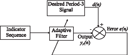The set of equations that describe the RLS algorithm is as follows: \documentclass{aastex}\usepackage{amsbsy}\usepackage{amsfonts}\usepackage{amssymb}\usepackage{bm}\usepackage{mathrsfs}\usepackage{pifont}\usepackage{stmaryrd}\usepackage{textcomp}\usepackage{portland,xspace}\usepackage{amsmath,amsxtra}\pagestyle{empty}\DeclareMathSizes{10}{9}{7}{6} \begin{document} \begin{align*} \begin{cases} k (n) = \frac {\lambda^ {- 1} P (n - 1) x (n)} {1 + \lambda^ {- 1} x^T (n) P (n - 1) x (n)} \\ y (n) = w^T (n - 1) x (n) \\ e (n) = d (n) - y (n) \\ w (n) = w (n - 1) + k (n) e (n)\\ P (n) = \lambda^ {- 1} [ P (n - 1) - k (n) x^T (n) P (n - 1) ] \end{cases} \tag {45} \end{align*} \end{document}

FIG. 5.

The block diagram of the adaptive algorithm.

where x(n) is the input to the filter, λ is the forgetting factor, 0 < λ < 1, y(n) is the output of the filter, w(n) is the weight vector, d(n) is the desired response signal, and e(n) is the estimated error between the output y(n) and the desired response d(n). k(n) is the gain vector (Eleftheriou and Falconer, 1986). The algorithm has been formulated based on computing the derivative of the objective function which is a function of the estimated error between the desired response and the output of the filter as follows: \documentclass{aastex}\usepackage{amsbsy}\usepackage{amsfonts}\usepackage{amssymb}\usepackage{bm}\usepackage{mathrsfs}\usepackage{pifont}\usepackage{stmaryrd}\usepackage{textcomp}\usepackage{portland,xspace}\usepackage{amsmath,amsxtra}\pagestyle{empty}\DeclareMathSizes{10}{9}{7}{6} \begin{document} \begin{align*} J (n) = \sum_{i = 0}^n \lambda^{n - i} \left| d (i) - w^T (n) x (i) \right| ^2 \tag{46} \end{align*} \end{document}

Computing the derivative of the objective function J(n) with respect to the weight w(n) and assigning it to zero yields: \documentclass{aastex}\usepackage{amsbsy}\usepackage{amsfonts}\usepackage{amssymb}\usepackage{bm}\usepackage{mathrsfs}\usepackage{pifont}\usepackage{stmaryrd}\usepackage{textcomp}\usepackage{portland,xspace}\usepackage{amsmath,amsxtra}\pagestyle{empty}\DeclareMathSizes{10}{9}{7}{6} \begin{document} \begin{align*} \frac {\partial J (n)} {\partial w (n)} = 0\end{align*} \end{document} \documentclass{aastex}\usepackage{amsbsy}\usepackage{amsfonts}\usepackage{amssymb}\usepackage{bm}\usepackage{mathrsfs}\usepackage{pifont}\usepackage{stmaryrd}\usepackage{textcomp}\usepackage{portland,xspace}\usepackage{amsmath,amsxtra}\pagestyle{empty}\DeclareMathSizes{10}{9}{7}{6} \begin{document} \begin{align*} w (n) = \left[ \sum_{i = 0}^n \lambda^{n - i}x (i) x^T (i) \right] ^{- 1} \left[ \sum_{i = 0}^nx (i) d (i) \right] \tag{47} \end{align*} \end{document}

d(n) is chosen to represent a period-3 signal; therefore, a sine wave signal with frequency ω = 2π/3 is considered as the desired response of the filter. In frequency response, the sine wave represents only one frequency component represented by the frequency of the signal. Therefore, if a sine wave with frequency ω = 2π/3 is chosen, it will represent a pure period-3 component. d(n) will adjust the weights so that the filter extracts the period-3 property from the input signal and eliminates the other frequency components.

The algorithm for extracting the period-3 spectrum by this technique is summarized in Algorithm 6.

Algorithm 6

Z curve-based coding region prediction algorithm

1.	Convert the DNA sequence into three sequences x₁(n), y₁(n) and z₁(n) as given by formula (44).
2.	Compute the output y_F(n), \documentclass{aastex}\usepackage{amsbsy}\usepackage{amsfonts}\usepackage{amssymb}\usepackage{bm}\usepackage{mathrsfs}\usepackage{pifont}\usepackage{stmaryrd}\usepackage{textcomp}\usepackage{portland,xspace}\usepackage{amsmath,amsxtra}\pagestyle{empty}\DeclareMathSizes{10}{9}{7}{6}\begin{document}$$F \in \{x_1, y_1, z_1 \} $$\end{document} , by RLS algorithm represented by the set of equations in (45)
3.	Compute the total output Y(n) as a linear combination of the power spectra of the three output signals as indicated by:
	\documentclass{aastex}\usepackage{amsbsy}\usepackage{amsfonts}\usepackage{amssymb}\usepackage{bm}\usepackage{mathrsfs}\usepackage{pifont}\usepackage{stmaryrd}\usepackage{textcomp}\usepackage{portland,xspace}\usepackage{amsmath,amsxtra}\pagestyle{empty}\DeclareMathSizes{10}{9}{7}{6} \begin{document} \begin{align} Y (n) = \mid y_{x_1} (n) \mid^2 + \mid y_{y_1} (n) \mid^2 + \mid y_{z_1} (n) \mid^2 \tag{48} \end{align} \end{document}

The technique does not use the DFT. In addition, no sliding window is used in this technique since a sequence is processed by the adaptive filter as one unit. The method is not data-driven since there is no statistical or learning data is required in the processing of sequences. Regarding the complexity of the method, the algorithm is recursive and the complexity of the iteration is O(N), where N is the length of the sequence. The number of weight coefficients L is a parameter that has to be set and could affect the results. The forgetting factor λ is another parameter that has to be set (Ma and Zhu, 2007).

The disadvantage of the technique is that it uses a recursive algorithm which might need much iteration to adjust the weights of the filter until the error converges to a minimum value. In addition, the weights are adjusted for each individual representation sequence.

2.9. Signal boosting

Gunawan et al. (2007) proposed a technique that enhances the period-3 spectrum of coding regions in DNA sequences and suppresses the period-3 spectrum of non-coding regions to improve the prediction of coding regions of DNA sequences. In this technique, a DNA sequence is mapped to four binary indicator sequences. The DFT is calculated for a Bartlett sliding window of length L of the sequences as follows: \documentclass{aastex}\usepackage{amsbsy}\usepackage{amsfonts}\usepackage{amssymb}\usepackage{bm}\usepackage{mathrsfs}\usepackage{pifont}\usepackage{stmaryrd}\usepackage{textcomp}\usepackage{portland,xspace}\usepackage{amsmath,amsxtra}\pagestyle{empty}\DeclareMathSizes{10}{9}{7}{6} \begin{document} \begin{align*} X_l [k ] = \sum_ {n = 0} ^ {L - 1} x_l [ n ] w [ n ] e^ {- j \frac {2 \pi n k} {L}} \tag {49} \end{align*} \end{document}

where w[n] is a Bartlett window with length L, \documentclass{aastex}\usepackage{amsbsy}\usepackage{amsfonts}\usepackage{amssymb}\usepackage{bm}\usepackage{mathrsfs}\usepackage{pifont}\usepackage{stmaryrd}\usepackage{textcomp}\usepackage{portland,xspace}\usepackage{amsmath,amsxtra}\pagestyle{empty}\DeclareMathSizes{10}{9}{7}{6}\begin{document}$$l \in \{A, C, G, T \} $$\end{document} , and x_l[n] is a sliding window of the sequence of nucleotide l with length L. The Bartlett window is very similar to the triangular window except that it ends with zeros at samples 1 and L, whereas the triangular window ends with nonzero values at those samples. The advantage of the Bartlett window is to eliminate extraneous peaks that appear due to background noise. The spectrum of a DNA sequence is calculated by summing the spectra of the four nucleotides as follows: \documentclass{aastex}\usepackage{amsbsy}\usepackage{amsfonts}\usepackage{amssymb}\usepackage{bm}\usepackage{mathrsfs}\usepackage{pifont}\usepackage{stmaryrd}\usepackage{textcomp}\usepackage{portland,xspace}\usepackage{amsmath,amsxtra}\pagestyle{empty}\DeclareMathSizes{10}{9}{7}{6} \begin{document} \begin{align*} S [k ] = \mid X_A [ k ] \mid^2 + \mid X_C [ k ] \mid^2 + \mid X_G [ k ] \mid^2 + \mid X_T [ k ] \mid^2 \tag{50} \end{align*} \end{document}

The value of S[L/3], which represents the 3-base periodicity, is stored as follows: \documentclass{aastex}\usepackage{amsbsy}\usepackage{amsfonts}\usepackage{amssymb}\usepackage{bm}\usepackage{mathrsfs}\usepackage{pifont}\usepackage{stmaryrd}\usepackage{textcomp}\usepackage{portland,xspace}\usepackage{amsmath,amsxtra}\pagestyle{empty}\DeclareMathSizes{10}{9}{7}{6} \begin{document} \begin{align*} \psi (m) = S_m [ L / 3 ], \quad m = 1, 2, \cdots, N - L \tag{51} \end{align*} \end{document}

where m is the position of the sliding window and N is the length of the DNA sequence.

A gain function, Γ(m), is calculated to enhance the period-3 spectrum at coding regions and attenuate it at non-coding regions. Γ(m) is calculated based on the spectrum, ψ(m), by estimating the signal-to-noise ratio SNR of the signal. The SNR is calculated by computing a short term average signal energy, P(m), as follows: \documentclass{aastex}\usepackage{amsbsy}\usepackage{amsfonts}\usepackage{amssymb}\usepackage{bm}\usepackage{mathrsfs}\usepackage{pifont}\usepackage{stmaryrd}\usepackage{textcomp}\usepackage{portland,xspace}\usepackage{amsmath,amsxtra}\pagestyle{empty}\DeclareMathSizes{10}{9}{7}{6} \begin{document} \begin{align*} P (m) = (1 - \alpha) P (m) + \alpha \cdot \psi (m) \tag{52} \end{align*} \end{document}

where α is a small positive constant, e.g., α = 0.2, which acts as a smoothing factor. An estimate of the noise floor level, Q(m), is also calculated as follows: \documentclass{aastex}\usepackage{amsbsy}\usepackage{amsfonts}\usepackage{amssymb}\usepackage{bm}\usepackage{mathrsfs}\usepackage{pifont}\usepackage{stmaryrd}\usepackage{textcomp}\usepackage{portland,xspace}\usepackage{amsmath,amsxtra}\pagestyle{empty}\DeclareMathSizes{10}{9}{7}{6} \begin{document} \begin{align*} Q (m) = \begin{cases} (1 + \beta) q (m - 1) \, \quad Q (m - 1) \leq P (m) \\ P (m) \qquad \qquad \ \, \ \quad Q (m - 1) > P (m) \end{cases} \tag{53} \end{align*} \end{document}

where β is a small positive constant, e.g., β = 0.0002, controlling how fast the noise floor level adapts to changes. For the initial state, P(1) = 0.5ψ(1) and Q(1) = 0.1.

The gain function at the base pair position m is the ratio of the SNR to the signal floor level as follows: \documentclass{aastex}\usepackage{amsbsy}\usepackage{amsfonts}\usepackage{amssymb}\usepackage{bm}\usepackage{mathrsfs}\usepackage{pifont}\usepackage{stmaryrd}\usepackage{textcomp}\usepackage{portland,xspace}\usepackage{amsmath,amsxtra}\pagestyle{empty}\DeclareMathSizes{10}{9}{7}{6} \begin{document} \begin{align*} \Gamma (m) = \frac {P (m)} {Q (m)} \tag {54} \end{align*} \end{document}

The boosted signal is then calculated as follows: \documentclass{aastex}\usepackage{amsbsy}\usepackage{amsfonts}\usepackage{amssymb}\usepackage{bm}\usepackage{mathrsfs}\usepackage{pifont}\usepackage{stmaryrd}\usepackage{textcomp}\usepackage{portland,xspace}\usepackage{amsmath,amsxtra}\pagestyle{empty}\DeclareMathSizes{10}{9}{7}{6} \begin{document} \begin{align*} \hat{\psi} (m) = \Gamma (m) \cdot \psi (m) \tag{55} \end{align*} \end{document}

The gain Γ(m) is limited to be no greater than 10 dB.

The boosted signal is applied to a neural network classifier to differentiate the coding from non-coding regions. The authors presented a multilayer neural network trained using a backpropagation algorithm for this purpose. The configuration of the network is 1-4-4-1 (Gunawan et al., 2007). The input to the network is a sample of the boosted signal, \documentclass{aastex}\usepackage{amsbsy}\usepackage{amsfonts}\usepackage{amssymb}\usepackage{bm}\usepackage{mathrsfs}\usepackage{pifont}\usepackage{stmaryrd}\usepackage{textcomp}\usepackage{portland,xspace}\usepackage{amsmath,amsxtra}\pagestyle{empty}\DeclareMathSizes{10}{9}{7}{6}\begin{document}$$\hat{\psi}_m$$\end{document} , and the output of the network is a coding or non-coding label for a particular region's nucleotide. According to the large amount of training data used, we suggest that this network architecture is too simple to be trained to differentiate between coding and non-coding regions. We postulate that a frame of the signal has to be presented to the network each time for training instead of a single sample element. In addition, the number of hidden units should be small to some extent so that the network can generalize in the training. Algorithm 7 summarizes the main steps of this technique.

Algorithm 7

Algorithm of the signal boosting technique

1.	Convert the DNA sequence into four binary indicator sequences corresponding to the four nucleotides
2.	Using a sliding window, compute the spectrum of each of the binary indicator sequences at frequency L/3 by formula (49)
3.	Compute the period-3 spectrum of the sequence ψ(m) as the sum of the power spectra of four indicator sequences
4.	Compute the short term signal energy P(m) and an estimate of the noise floor level Q(m) by formulas (52) and (53), respectively.
5.	Compute the gain function Γ(m) by formula (54)
6.	Calculate the boosted spectrum signal \documentclass{aastex}\usepackage{amsbsy}\usepackage{amsfonts}\usepackage{amssymb}\usepackage{bm}\usepackage{mathrsfs}\usepackage{pifont}\usepackage{stmaryrd}\usepackage{textcomp}\usepackage{portland,xspace}\usepackage{amsmath,amsxtra}\pagestyle{empty}\DeclareMathSizes{10}{9}{7}{6}\begin{document}$$\hat{\psi} (m)$$\end{document} by formula (55)
7.	Classify the boosted spectrum signal into coding and non-coding regions by an artificial neural network

The method is considered as data-driven since it uses learning data to train the neural network for clustering the spectrum signal. Since the method computes the spectrum using the DFT, we can say that the complexity of the technique is O(NL). We can also identify the complexity of training the neural network as \documentclass{aastex}\usepackage{amsbsy}\usepackage{amsfonts}\usepackage{amssymb}\usepackage{bm}\usepackage{mathrsfs}\usepackage{pifont}\usepackage{stmaryrd}\usepackage{textcomp}\usepackage{portland,xspace}\usepackage{amsmath,amsxtra}\pagestyle{empty}\DeclareMathSizes{10}{9}{7}{6}\begin{document}$$O ({\cal N}E)$$ \end{document} , where \documentclass{aastex}\usepackage{amsbsy}\usepackage{amsfonts}\usepackage{amssymb}\usepackage{bm}\usepackage{mathrsfs}\usepackage{pifont}\usepackage{stmaryrd}\usepackage{textcomp}\usepackage{portland,xspace}\usepackage{amsmath,amsxtra}\pagestyle{empty}\DeclareMathSizes{10}{9}{7}{6}\begin{document}$${\cal N}$$\end{document} is the number of epochs, and E is the amount of training data. The window length is a parameter that has to be set and its value affects the results. The optimum value of this parameter is usually different from one sequence to another.

Boosting the period-3 spectrum signal could eliminate background noise that might produce wrong exons in the prediction process. Using a neural network classifier might lead to more accurate prediction than using an apriori crude threshold since neural networks have a good reputation as a classifier if they are set properly and trained with sufficient data.

2.10. Model-based approach

Kahumani et al. (2008) proposed a technique considering that the 3-base periodicity is embedded in noise. Therefore, the task is to extract the period-3 component from the noisy signal using a statistically optimal null filter (SONF). The technique maximizes the signal-to-noise ratio of the output using an instantaneous matched filter (IMF), then the estimated signal is enhanced using a least-square optimization technique by minimizing the error between estimated noise and the noise of the input. Therefore, the algorithm computes a gain matrix P[m] and a scaling function λ[m]. The scaling function scales the output of the IMF filter to obtain a better approximation of the desired signal which is embedded in noise. Based on the recursive least square algorithm, the recursive algorithm for implementing the SONF is denoted as follows (Agarwal et al., 2001): \documentclass{aastex}\usepackage{amsbsy}\usepackage{amsfonts}\usepackage{amssymb}\usepackage{bm}\usepackage{mathrsfs}\usepackage{pifont}\usepackage{stmaryrd}\usepackage{textcomp}\usepackage{portland,xspace}\usepackage{amsmath,amsxtra}\pagestyle{empty}\DeclareMathSizes{10}{9}{7}{6} \begin{document} \begin{align*} \begin{cases} v [m ] = v [ m - 1 ] + x [ m ] \phi [ m ] \\ P [ m ] = P [ m - 1 ] - \frac {P [ m - 1 ] \phi [ m ] \phi^T [ m ] P [ m - 1 ]} {1 + \phi^T [ m ] P [ m - 1 ] \phi [ m ]} \\ \lambda [ m ] = p [ m ] \phi [ m ] \\ y [ m ] = v^T [ m ] \lambda [ m ] \end{cases} \tag {56} \end{align*} \end{document}

where x[m] is the input to the SONF, φ[m] is the basis function, v[m] is the output of the IMF filter, P[m] is the gain matrix, λ[m] is the scaling function, and y[m] is the output of the SONF. The block diagram of the SONF, shown in Figure 6, clarifies this algorithm. The basis function φ[m] is chosen so that it models the period-3 property of coding regions. Therefore, three basis functions with lengths equal to the length of the input sequence are used in the process. 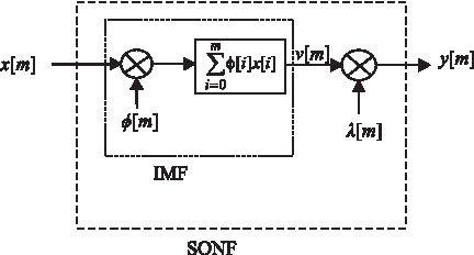The three functions correspond to the three possible reading frames and are given by: \documentclass{aastex}\usepackage{amsbsy}\usepackage{amsfonts}\usepackage{amssymb}\usepackage{bm}\usepackage{mathrsfs}\usepackage{pifont}\usepackage{stmaryrd}\usepackage{textcomp}\usepackage{portland,xspace}\usepackage{amsmath,amsxtra}\pagestyle{empty}\DeclareMathSizes{10}{9}{7}{6} \begin{document} \begin{align*} \phi_1 [ m] &= [100100100 \cdots ] \\ \phi_2 [ m ] &= [010010010 \cdots ] \\ \phi_3 [ m ] &= [001001001 \cdots ] \tag{57} \end{align*} \end{document}

FIG. 6.

The block diagram of statistically optimal null filter.

The coding region prediction algorithm for a DNA sequence of length N based on the SONF technique is summarized in Algorithm 8.

Algorithm 8

Algorithm of the model-based coding region prediction approach

1.	Set the position index l = 1.
2.	Select a window of length L nucleotides starting at position l of the DNA sequence
3.	Find the four binary indicator sequences x_A[m], x_C[m], x_G[m], and x_T[m] for the windowed sequence.
4.	Each of the four binary sequences is fed to a SONF and using the basis function, the corresponding outputs of the SONFs y_A[m], y_C[m], y_G[m], and y_T[m] are evaluated using the recursive formula (56).
5.	The SNR power gains G_A, G_C, G_G and G_T are computed as the ratio of the variance of the output of the SONF to the variance of the corresponding input, and then the total SNR gain G[l] is computed as the sum of these four power gains.
6.	The value of l is increased by 1, and if (l + L) is less than or equal to N, go to step 2.
7.	The peaks in G[l] represent the possible exon regions.

The algorithm computes the period-3 spectrum as the ratio of the variance of the output of the SONF to the corresponding input. This means that the filter tries to enhance the variance of the input signal by removing the background noise. Enhancing the variance means enhancing the biased distribution of the nucleotide in the three reading frames. This concept is related to the empirical explanation of Yin and Yau (2005) and the mathematical proof provided by Marhon and Kremer (2010) about the relationship of the period-3 spectrum property and the nucleotide distribution.

The method does not use the DFT in the analysis. It uses a sliding window, and like other window-based methods, setting the window length parameter could make the accuracy of the results different from one DNA sequence to another depending on the lengths of the exons in each sequence. The method is not data driven since there is no need for statistical or learning data in the analysis. We can identify the overall complexity of this technique to be O(NLK), where K is the number of iterations required to process the window by the filter. The window length L is a parameter that has to be set.

3. DSP-Based Gene Prediction Process

In this section, we break down the approaches used by the researchers that we described in the preceding section to create a generic DSP gene prediction model. This model serves as a common framework upon which the various approaches are built. By identifying the underlying common model, it will be easier to understand and relate the methods to each other. Furthermore, this framework will suggest new hybrid approaches and act as a guide for future processes. Most of the techniques of gene prediction that are based on the DSP analysis follow specific steps in analyzing symbolic DNA sequences to predict coding regions. Figure 1 has shown the generic block diagram of the gene prediction process based on DSP analysis.

Step 1: Mapping DNA sequences

Usually, the first step in the process is to convert symbolic DNA sequences into numerical sequences since DSP tools can process only numerical entities. Symbolic DNA sequences are mapped to numerical sequences while retaining the biological meaning of the represented information. In other words, the conversion is done in a way so that the original DNA sequence can be retrieved from the numerical information.

Step 2: Sequence windowing

The next step in the process is the windowing system. Most of the techniques analyze DNA sequences based on a walking window basis. This is necessary because the recognition of genes is impossible from single nucleotides, yet is a location specific process across extended DNA sequences. The windowing system of processing DNA sequences is different from one technique to another. According to the window basis, a rectangular window or any other shape with a specific length of base pairs is processed at a time. Then the window is slid by one or more base pair positions along the sequence, and the processing is repeated on that window until the end of the sequence. It has been shown that the window shape and length parameters affect the prediction results (Akhtar et al., 2008b,c). Tiwari et al. (1997), Anastassiou (2000), and Kotlar and Lavner (2003) used a rectangular window in the analysis of DNA sequences using the DFT tool. However, Gunawan et al. (2007) and Akhtar et al. (2008b) respectively used Bartlett and Kaiser windows in their methods in order to eliminate the edges that are produced with the rectangular window. Other window shapes such as Gaussian, Hamming, Hanning, and Blackman could also be used. Figure 7 shows various window shapes with length L. Akhtar et al. (2008b) analyzed the use of these window shapes by comparing the area under the receiver operating characteristic (ROC) curve. According to their experiment, the performance of Blackman and Hanning is poor in gene prediction. On the other hand, the rectangular window causes the power of the STFT to leak over the adjacent frequencies. Akhtar et al. (2008b) have also shown that the window length parameter affects the results and its optimum value depends on the lengths and the number of exons in the sequence. According to these findings, we propose here optimizing the window shape and length for each biomolecular sequence under consideration to maximize the prediction accuracy in an adaptive way. Optimizing those two parameters will eliminate their effect on prediction results with the variation of biomolecular sequences.

FIG. 7.

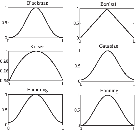
A diagram shows various window shapes.

Step 3: Period-3 spectrum extraction

Different techniques adopt different analysis tools in investigating the spectral properties of DNA sequences. These tools vary in their performance and computational complexities. Some tools, for example, the STFT, analyze genomic sequences based on a sliding window (Tiwari et al., 1997; Anastassiou, 2000), while other tools analyze a sequence as one unity (Mena-Chalco et al., 2008). Filtering is one of the tools that are also used in extracting a period-3 component in DNA sequences. In addition, some analysis tools process genomic data in the time domain, while others process sequences in the frequency domain. As a result, all the tools that are used to predict coding regions based on spectral analysis try to extract the period-3 component from the spectrum band of DNA sequences and enhance this frequency component in coding regions while attenuating the background noise in non-coding regions. Some tools are considered data-driven since they depend on experimental data or learning data in the analysis.

Step 4: Classification

After extracting the period-3 property, sequences are classified as coding and non-coding regions. Classification can be performed using a learning approach or a threshold. Thresholding is considered one of the major challenges in this field since threshold values could be different from one sequence to another. Some authors have determined experimental thresholds for their measures depending on experimental implementations (Yin and Yau, 2007). Other authors have computed a threshold value intrinsically based on the sequence to be predicted (Jiang et al., 2008).

We now map the methods described in Section 2 into the new framework. Table 1 presents the details of the stages of the gene prediction process followed by the ten techniques that we focus on in this study. In the following subsections, we analyze the differences between these techniques according to each stage in the prediction process.

Table 1.

Details of the Reviewed Gene Prediction Techniques

Technique	Representation method	Windowing system	Analysis tool	Classifier/threshold	Data driven	Exon length suitability	Reference
SCM	Voss	Window	DFT	Apriori threshold	No	Long/short (>100bp)	Tiwari et al. (1997)
OSCM	Optimized parameters	Window	DFT	None	No	Not stated	Anastassiou (2000)
SRM	Voss	Window	Spectral argument	None	Yes	Long/short	Kotlar and Lavner (2003)
EPND	None	Accumulative computation	Nucleotide distribution	Apriori threshold	No	Long	Yin and Yau (2007)
P(L)^(A) predictor	2D representation graph	Adjustable window length	DFT	Intrinsic threshold	No	Long/short	Jiang et al. (2008)
PWSR	Paired numerical	Window	DFT/statistics	None	Yes	Not stated	Akhtar et al. (2008a)
AMDF	Voss	Window	Filtering/magnitude averaging	None	No	Long/short	Akhtar et al. (2008a)
TDP	Voss	Window	Filtering/periodogram	None	No	Long/short	Akhtar et al. (2008a)
MGWT	Voss	Whole sequence	Wavelet	Apriori threshold	No	Long/short	Mena-Chalco et al. (2008)
RLS	Z curve	Whole sequence	Adaptive filter	None	No	Not stated	Ma and Zhu (2007)
Signal boosting	Voss	Bartlett window	DFT/signal boosting	NN classifier	Yes	Not stated	Gunawan et al. (2007)
SONF	Voss	Rectangular window	SONF	None	No	Long/short	Kahumani et al. (2008)

3.1. Representation method

A number of DSP-based coding region prediction techniques have been recently proposed and are discussed in this article. In order to apply digital signal processing tools to DNA sequences, symbolic sequences must first be converted into a numerical representation. Several representation schemes have been proposed to represent DNA sequences. Table 2 shows the most popular representation schemes used to convert DNA sequences into numerical sequences in order to analyze them using DSP tools. These schemes have taken into consideration some biological properties of nucleotides in order to preserve the biological meaning of the mapped information. One of these schemes is to give each nucleotide an equal weight since there is no biological evidence which says that one nucleotide is more important than another even though some researchers have optimized the parameters corresponding to the four nucleotides (Anastassiou, 2000). Another property that has been considered in some representation schemes is the classification of purine(A,G)/pyrimidine (C,T) and the strength of the hydrogen bond. This property has been considered in the representation that uses complex numbers (Cristea, 2002). In general, avoiding redundancy and degeneracy has been taken into consideration in representation schemes. In addition, there is coordination between the representation and the DSP tool applied to the numerical data.

Table 2.

Details of Some DNA Sequence Representation Schemes

Technique	Numerical sequences	Description	Type
Voss	Four indicator sequences	The presence of a nucleotide is represented by 1, and the absence is represented by 0	Real
Z curve	Three sequences represent 3D curve	Each base pair is represented by a 3D vertex in a 3D curve	Real
2D dynamic representation	Two sequences	2D dynamic graphical representation	Real
Universal graphical representation	Four complex sequences	Four 2D vectors represent the four nucleotides	Complex
Optimized parameters	Four complex sequences	Four complex parameters are optimized to represent the four nucleotides	Complex
Complex representation	Four complex sequences	Four complex numbers represent the four nucleotides	Complex
Paired numerical representation	Two sequences correspond to the A-T and G-C nucleotides	The presence of a nucleotide is represented by 1, and the absence is represented by 0	Real
DV-curve	A sequence of Cartesian coordinates	Each nucleotide is represented by dual 2D vectors	Real

Voss (1992) proposed a technique in which a symbolic sequence composed of K symbols can be decomposed into K binary sequences. This technique solves the problem of correlation that occurs between bases of DNA sequences when the number of dimensions is less than four. In DNA sequences, a genomic sequence is decomposed into four binary indicator sequences corresponding to the four nucleotides. The presence of a nucleotide at a particular base pair position is represented by 1, and the absence of it is represented by 0. Figure 8 shows the diagram of the Voss representation of the DNA sequence for the mouse β-globin exon-1 [GenBank:J00413]. The diagram represents the presence of a nucleotide at a particular base pair position as a high-level pulse and the absence as a low-level pulse.

FIG. 8.

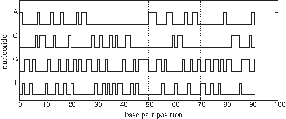
A diagram shows the Voss representation of the DNA sequence for the mouse β-globin exon-1 [GenBank:J00413].

Zhang and Zhang (1994) proposed decomposing a DNA sequence into three series of digital signals in a technique called Z curve representation. The numerical values of these series consist of −1 and +1. The three series have clear biological meanings. The first series characterizes the distribution of the bases as purine and pyrimidine. The second series characterizes the distribution of the amino/keto type of the bases along a DNA sequence. The third series characterizes the distribution of the strength of the hydrogen bond (weak/strong) of bases along the DNA sequence. Therefore, the molecular characteristics are retained and represented with only three series of digital values (Yan et al., 1998). Figure 9 shows the 3D graph of the Z curve representation of the DNA sequence for the mouse β-globin exon-1 [GenBank:J00413]. The 3D graph is constructed as the vector addition of the voxels corresponding to the nucleotides in the DNA sequence.

FIG. 9.

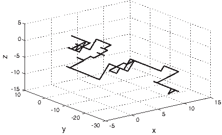
3D graph of the Z curve representation of the DNA sequence for the mouse β-globin exon-1 [GenBank:J00413]. Each base pair is represented by a 3D point (x,y,z).

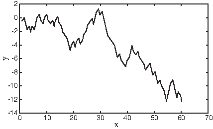
Bielinska-Waz et al. (2007) proposed a 2D-dynamic graphical representation method. In this technique, material points with different masses represent DNA sequences in the 2D space. The method eliminates the degeneracies that occurred in a previous method (Nandy, 1994) which the proposed method has depended on. The method distinguishes between the graphical points that are visited more than one time by an integer index called the mass. In addition, the simplicity of the original model, in Nandy (1994), is retained (Bielinska-Waz et al., 2007). Figure 10 shows the 2D graph of the 2D-dynamic representation of the DNA sequence for the mouse β-globin exon-1 [GenBank:J00413].

FIG. 10.

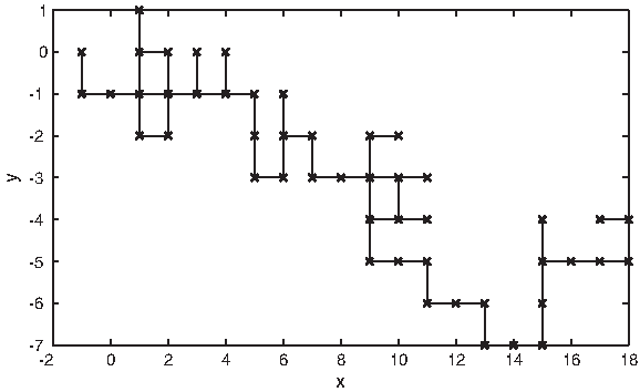
A 2D dynamic graph of the DNA sequence for the mouse β-globin exon-1 [GenBank:J00413]. The x-axis represents the real part of the complex value, and the y-axis represents the imaginary part of the complex value.

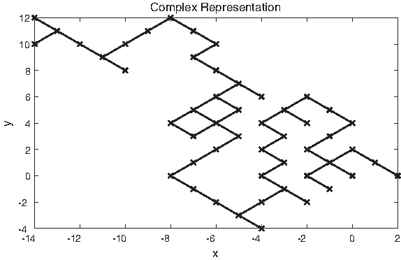
Yau et al. (2003) proposed a graphical representation method to convert symbolic DNA sequences into a 2D graph. The four nucleotides are represented by four 2D vectors in the first and fourth quarters. They determined specific Cartesian coordinates of vectors. Jiang et al. (2008) modified this method by determining the Cartesian coordinates of the four vectors by an angle θ. Jiang et al. (2008) used different values of θ for different sequences when they analyzed these sequences by the DFT to predict their coding regions. The Cartesian coordinates of the four vectors are considered as complex numbers when sequences are analyzed by DSP tools. The problem is that θ is a parameter that has to be set. Figure 11 shows a diagram of the graphical representation of the DNA sequence for the mouse β-globin exon-1 [GenBank:J00413] with θ = π/3. In this graph, each point, corresponding to a nucleotide at a particular base pair position, is evaluated as the vector addition of the previous points, corresponding to the previous nucleotides in the previous base pair positons of the biomolecular sequence.

FIG. 11.

A 2D graph of the universal graphical representation of the DNA sequence for the mouse β-globin exon-1 [GenBank:J00413]. The x-axis represents the real value of the complex value, and the y-axis represents the imaginary part of the complex value.

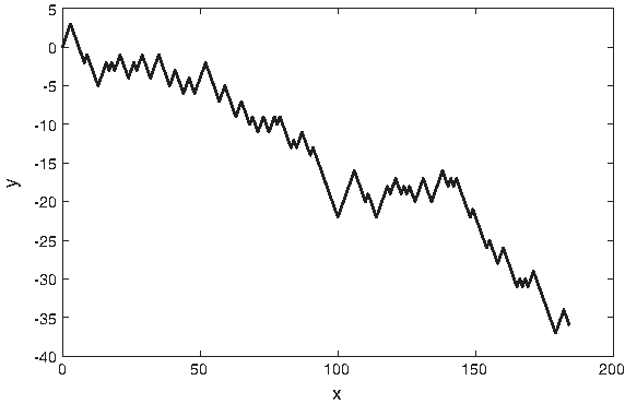
Anastassiou (2000) optimized four parameters corresponding to the four nucleotides to obtain maximum differentiation between the period-3 spectrum of coding and non-coding regions. A DNA sequence is converted to four complex sequences corresponding to the four nucleotides. The presence of a nucleotide is represented by the value of the corresponding optimized parameter, and the absence of it is represented by 0. Anastassiou (2000) used the optimized parameters in the OSCM that he proposed. The optimized values may not give good results if they are applied with other techniques such as the SCM since the objective function used in the optimization problem is based on the OSCM as given in formula (4). Figure 12 shows the optimized complex representation of the DNA sequence for the mouse β-globin exon-1 [GenBank:J00413] in the complex plane.

FIG. 12.

A 2D graph of the optimized complex representation of the DNA sequence for the mouse β-globin exon-1 [GenBank:J00413]. The x-axis represents the real part of the complex value, and the y-axis represents the imaginary part of the complex value.

The complex representation is another method which is similar to the Voss representation except it represents the presence of a nucleotide by a complex number instead of 1 (Cristea, 2002; Anastassiou, 2000). In this representation, the features of the bases have been retained by translating them into mathematical properties. For example, the complex numbers of the pairs A-T and C-G are complex conjugate and this emulates the property of the two strands that form the DNA molecule. In addition, the purine and pyrimidine bases have equal imaginary parts and equal real parts with an opposite sign. Figure 13 shows the complex representation of the DNA sequence for the mouse β-globin exon-1 [GenBank:J00413] in the complex plane.

FIG. 13.

A 2D graph of complex representation of the DNA sequence for the mouse β-globin exon-1 [GenBank:J00413]. The x-axis represents the real part of the complex value, and the y-axis represents the imaginary part of the complex value.

Akhtar et al. (2007a) proposed a numerical representation technique that assigns the values +1 and −1 to the presence of the A-T and C-G nucleotides. This representation is based on statistical evidence that says introns are rich in nucleotides A and T, while exons are rich in nucleotides C and G (Cristea, 2002). Therefore, Akhtar et al. (2007a) employed this representation to predict coding regions in DNA sequences.

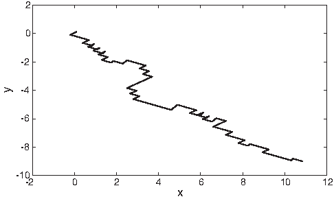
Zhang (2009) proposed a new representation method in which each nucleotide is represented by dual 2D vectors. For a DNA sequence, a DV-curve is constructed according to a mathematical model. The DV-curve visualizes the sequence without loss of information. The DV-curve reflects the length of the sequence. It also reflects useful information such as mutation (Zhang, 2009). Figure 14 shows the 2D graph of the DV-curve mapping of the DNA sequence for the mouse β-globin exon-1 [GenBank:J00413].

FIG. 14.

A 2D graph of the DV curve representation of the DNA sequence for the mouse β-globin exon-1 [GenBank:J00413]. The x and y values represent the coordinates of a 2D vector.

In the SCM, Tiwari et al. (1997) used the Voss representation to convert symbolic DNA sequences to numerical sequences in order to process them by the STFT. Based on this representation scheme, they proposed their SCM given in formula (1) to extract the 3-base periodicity of coding regions (Tiwari et al., 1997). Kotlar and Lavner (2003) also depended on the Voss representation to propose their SRM given in formula (8). This technique computes the argument of the DFT of each of the four binary indicator sequences at frequency f = 1/3 based on the number of occurrences of the corresponding nucleotide in the three reading frames.

Yin and Yau (2007) did not convert symbolic DNA sequences into numerical representation since their technique, EPND, is based on the nucleotide distributions in a DNA sequence. Thier technique, however, uses the Voss representation in origin since formula (16), used to compute the period-3 spectrum, has been derived based on the DFT and the Voss representation (Marhon and Kremer, 2010). They could compute the 3-base periodicity at each nucleotide position based on the variance in the distributions of the four nucleotides. They did not need to map DNA sequences to a numerical representation and use the STFT like other DFT-based methods.

In the W(j, L) and P(L) predictors, Jiang et al. (2008) used the 2D representation graph to represent DNA sequences as numerical series. The 2D representation graph was presented by Yau et al. (2003). The method assigns a 2D Cartesian vector to each nucleotide. The method does not cause degeneracy; otherwise, there will be loss of biological information. In addition, the graphical representation is universal, which means there is a one-to-one correspondence between the graph and the original DNA sequence. The amplitude of each point in the representation graph represents the sum of the amplitudes of the preceding nucleotides; therefore, the difference between the amplitudes of two points represents the change in the distributions of the nucleotides. Jiang et al. (2008) represented the graphical representation vectors as complex numbers to transform a DNA sequence to four sequences as in formula (21). This representation is similar to the representation (optimized complex numbers) of Anastassiou (2000) used in the OSCM except that, in the former, the real and imaginary parts are evaluated as trigonometric functions (sin and cos) of θ. Using complex numbers increases the computation time when the DFT is applied, but it could improve the accuracy of the results by differentiating more effectively between the spectrum of coding and non-coding regions when 3-base periodicity is investigated.

In their PWSR measure, Akhtar et al. (2008a) used the paired-numerical representation that they proposed in Akhtar et al. (2007a). This representation pairs the nucleotides A and T in one representation and the nucleotides C and G in another representation. This pairing is based on the statistical property that exons are rich in nucleotides C and G, while introns are rich in nucleotides A and T (Cristea, 2002). The values +1 and −1 are used to denote A-T and C-G nucleotide pairs respectively. This could give more differentiation between exon and intron regions when the 3-base property is investigated. It could decrease the computation time compared with Voss representation since two numerical sequences are used instead of four. Akhtar et al. (2008a) also used the Voss representation with the time-domain algorithms AMDF and TDP. They used the Voss representation here because it is more appropriate to apply such algorithms to the four binary indicator sequences than other representation schemes. These algorithms extract the 3-base periodicity of each binary indicator after removing other frequency components by filtering.

In the MGWT, Mena-Chalco et al. (2008) applied the modified Gabor-Wavelet transform to a DNA sequence after converting it to four binary indicator sequences (Voss). Their technique is based on filtering each binary indicator sequence separately by keeping the period-3 component and removing other components. Filter coefficients are computed based on the modified Gabor-Wavelet basis function shown in formula (39). Then they transformed the coefficients to the time-domain using the inverse Fourier transform. Filtering each indicator sequence is done by convoluting the sequence by the filter coefficients vector at different scales. The authors analyzed each nucleotide sequence after mapping it to a sequence of numbers.

In the Z curve method, Ma and Zhu (2007) exploited the Z curve representation in the RLS algorithm for gene prediction. The Z curve is a 3D curve representation for a given DNA sequence. The Z curve coordinates and the Voss representation are related as a pair of linear transformations as denoted in formula (44). x₁(n), y₁(n) and z₁(n) take the digital values 1 and −1. x₁(n) takes the value 1 when the n^th base is a purine (A or G), or −1 when the n^th base is a pyrimidine(T or C). y₁(n) takes the value 1 when the n^th base is amino-type (A or C), or −1 when the n^th base is keto-type (T or G). z₁(n) is equal to 1 when the n^th base represents a weak hydrogen bond (A or T), or −1 when the n^th base represents a strong hydrogen bond (G or C). They justified the use of this representation scheme because it contains all the biological information of a DNA sequence. It was shown that a DNA sequence and its Z curve representation can be reconstructed from each other (Yan et al., 1998). Mapping a DNA sequence to three digital sequences reduces the computation time compared with the Voss representation. In the signal boosting and the SONF methods, Gunawan et al. (2007) and Kahumani et al. (2008), respectively, used the Voss representation to map DNA sequences to a numerical form. Gunawan et al. (2007) justified the use of the Voss representation for its simplicity and popularity.

3.2. Windowing system

DFT-based gene prediction methods differentiate between coding and non-coding regions by measuring the spectrum at f = ⅓. These methods apply the STFT to a rectangular window of length L of a DNA sequence and compute the power spectrum at frequency L/3. The window is successively shifted by one base pair position along the sequence, and the spectrum is recomputed (Tiwari et al., 1997; Anastassiou, 2000). The window size should be chosen carefully. An excessively small window size emphasizes the small peaks of background noise, while an excessively large window size results in missing short exons and introns (Tiwari et al., 1997; Akhtar et al., 2008b). These two cases affect the prediction accuracy. Other DSP-based methods that measure the 3-base periodicity without computing the DFT sometimes do not use a sliding window in the analysis of DNA sequences (Yin and Yau, 2007; Mena-Chalco et al., 2008).

In the SCM, Tiwari et al. (1997) used a sliding window in the analysis of DNA sequences using the STFT. They used a rectangular window with a length of 351 bp in the analysis. They stated that a window length of 250–400 bp gives similar results, and with a window length of 351 bp, the number of false negatives is minimized. When the window length was less than 250, noise was emphasized. On the other hand, some exons are missed when the window length is greater than 400 bp due to the overlap between regions. Anastassiou (2000), in the OSCM, also used a rectangular window in the analysis by the STFT. He used a sliding window with a length of 351 bp. Kotlar and Lavner (2003), in the SRM, used a sliding frame in the analysis and tested their method with different frame lengths. They commented that analyzing DNA sequences using short frames results in detecting small exons and introns, while analyzing sequences using long frames results in missing them. On the other hand, using short frames increases false positives and negatives. According to their comment, the accuracy of the SRM is also affected by the window or frame length, and this is clear since this measure also depends on the asymmetry of nucleotides in the three reading frames in computing the spectral rotation as given in formulas (8) and (7).

In the EPND technique, Yin and Yau (2007) computed the SNR of a DNA sequence at each base pair position k as the ratio of the 3-base periodicity at that position to the length of the DNA walk sequence which is the subsequence from the beginning of the DNA sequence to the k^th base pair. The computation of the SNR was given in formula (17). The authors computed the distributions of the four nucleotides at the three reading frames along a DNA sequence accumulatively (Yin and Yau, 2007). In other words, the nucleotide distributions of a DNA walk sequence of length k were calculated recursively from the previous calculations of the DNA walk sequence of length k − 1 with the frequencies of the nucleotides in the position k. This has reduced the computational complexity of the technique.

For long DNA sequences that contain more than two exons or two introns, the accumulated SNR of the last exon will be low especially when the preceding intron is long. According to the algorithm mentioned in Section 2.4, the SNR of this exonic region will not exceed the predetermined threshold, and this might affect the prediction accuracy. Therefore, to overcome this problem, the authors suggested partitioning a long DNA sequence if it is longer than 2000 bp. However, a problem might emerge if the partitioning point is set in the middle of an exon since each part of the exon will be analyzed in a different partition. There is another problem with the accumulative computation of SNR; a short exon between two long introns or a short intron between two long exons might be missed, and this affects the accuracy of prediction.

Jiang et al. (2008), in their approach P(L), used a rectangular window to calculate the 3-base periodicity spectrum using the DFT. The difference between their approach and other DFT-based approaches that adopt a sliding window is that they use an arbitrary window length for the initial analysis. Then they recompute the window length depending on the lengths of the exons predicted by the arbitrary window length analysis. They proposed that the modified window length is the average of the lengths of the initially predicted exons. This could improve the prediction accuracy since the optimum window length should be close to the lengths of the exons to be predicted.

In the TFDM, Akhtar et al. (2008b) used a Kaiser sliding window with the PWSR measure and a rectangular sliding window with the AMDF measure, and combined the outputs of the two measures to form the total output of the hybrid method. With the PWSR measure, they tested different window shapes by comparing the area under the ROC curve. Their results showed that the Kaiser window has better performance than other window shapes. In the AMDF measure, a rectangular sliding window is also used to compute the 3-base periodicity in the time domain after performing bandpass filtering on numerical sequences.

It has been shown that the window length parameter has a significant effect on the prediction accuracy (Liew et al., 2005). Therefore, Mena-Chalco et al. (2008), in their MGWT technique, aimed to eliminate the dependency of the accuracy of prediction results on the window length parameter. In their technique, they used an analyzing function with 40 scale values determined as equal steps within a range. They truncated the length of the function to 1200 sequence points. Then, they convoluted each of the four binary sequences by the function sequence without using a sliding window. Even though the effect of the window length parameter has been eliminated in this technique, other parameters have been presented in the technique such as the lower and upper bounds of the scale range, which could affect the accuracy of the results. The authors state that short coding regions should be analyzed with small scales and long coding regions should be analyzed with large scales (Mena-Chalco et al., 2008). This implies that the scale range is a parameter that affects results. In addition, when a scale range is used, it is used with the analysis of the whole sequence which might include short and long coding regions. However, the effect of the scale range parameter might not be as much as the effect of the window length parameter.

Ma and Zhu (2007), in the RLS technique, analyzed the whole sequence by an adaptive filter. After converting a DNA sequence to the Z curve representation, they apply each Z curve sequence to the adaptive filter to extract the 3-base periodicity spectrum without applying the DFT. Kahumani et al. (2008), in the SONF method, also used filtering to remove embedded noise in DNA signals and keep period-3 components. They used a rectangular sliding window in their technique. The output of the SONF is a filtered window of the corresponding input window. The method has a high computational complexity since it involves a sliding window and a recursive algorithm applied successively.

Like other DFT-based methods, Gunawan et al. (2007), in the signal boosting technique, used a sliding window to calculate the 3-base periodicity spectrum of a DNA sequence, and then they boosted the spectrum signal to eliminate background noise. They used a Bartlett window to eliminate small peaks that are produced with the rectangular window. In their work, they fixed the window length parameter to be 351 bp, which was adopted in the OSCM (Anastassiou, 2000) and in other DFT-based methods.

3.3. Analysis tool

Almost all DSP-based gene prediction techniques depend on the analysis of the spectral characteristics of DNA sequences. These spectral characteristics include the 3-base periodicity of these sequences due to an unbalanced distribution of the four nucleotides in the three reading frames in coding regions. Amino acids have redundant codes which are combinations of three consecutive base pairs. The unbalanced distribution of the nucleotides in the three reading frames is due to the preference of amino acids for specific codes in coding regions and/or the biased usage of amino acids in proteins (Fickett, 1982; Tsonis et al., 1991). Most of the techniques use the DFT to analyze the 3-base periodicity of DNA sequences (Tiwari et al., 1997; Anastassiou, 2000). Other techniques used other tools, but the goal is the same which is analyzing the 3-base periodicity of DNA sequences to differentiate between coding and non-coding regions (Yin and Yau, 2007; Mena-Chalco et al., 2008; Ma and Zhu, 2007; Kahumani et al., 2008). Some gene prediction techniques use training data or parameters calculated experimentally (Solovyev et al., 1995; Burge and Karlin, 1997; Krogh, 1997; Kotlar and Lavner, 2003). These techniques are called data-driven techniques. In these techniques, the accuracy of the results depends on the amount of data used in training and the diversity of the sources (organisms) of data (Akhtar et al., 2008a). The advantage of training-free methods is that the methods work well when there is a lack of previous knowledge about the species under analysis, and these methods can annotate novel genomic sequences (Mena-Chalco et al., 2008).

In the SCM, Tiwari et al. (1997) proposed their measure given in formula (1) to compute the spectrum at frequency f = ⅓. This measure has become the basis for different techniques that have been proposed later on (Jiang et al., 2008; Mena-Chalco et al., 2008; Gunawan et al., 2007). In this technique, a DNA sequence is converted into four binary sequences to be analyzed by the DFT and the total Fourier spectrum of the sequence is computed as the sum of the spectra of the four binary sequences as given in formula (1). The technique did not handle the background noise in intronic regions. In addition, the effect of the rectangular window wasn't studied. In order to compare the spectra of coding and non-coding regions at frequency f = ⅓, Tiwari et al. (1997) calculated the SNR of the peak at f = ⅓ as the ratio of the spectrum at f = ⅓ to the average of the spectrum at all frequencies. Tiwari et al. (1997) showed that the average of the total spectrum \documentclass{aastex}\usepackage{amsbsy}\usepackage{amsfonts}\usepackage{amssymb}\usepackage{bm}\usepackage{mathrsfs}\usepackage{pifont}\usepackage{stmaryrd}\usepackage{textcomp}\usepackage{portland,xspace}\usepackage{amsmath,amsxtra}\pagestyle{empty}\DeclareMathSizes{10}{9}{7}{6}\begin{document}$$\overline{S}$$\end{document} can be calculated as given in formula (3). We think that this formula does not really reflect the average of the power spectrum. According to the experimental analysis of the average power spectrum of several DNA sequences, it is equal to N: \documentclass{aastex}\usepackage{amsbsy}\usepackage{amsfonts}\usepackage{amssymb}\usepackage{bm}\usepackage{mathrsfs}\usepackage{pifont}\usepackage{stmaryrd}\usepackage{textcomp}\usepackage{portland,xspace}\usepackage{amsmath,amsxtra}\pagestyle{empty}\DeclareMathSizes{10}{9}{7}{6} \begin{document} \begin{align*} \overline {S} = \frac {1} {N} \sum_ {k = 1} ^ {N} S (k / N) \approx N \tag {58} \end{align*} \end{document}

Anastassiou (2000), in the OSCM, also used the STFT in the analysis of DNA sequences. He assumed that the sum S, in formula (4), of the multiplication of each of the four Fourier coefficients U_A(N/3), U_C(N/3), U_G(N/3) and U_T(N/3) by four parameters a, c, g and t respectively can be considered as a complex random variable and its properties are based on the choice of the parameters a, c, g and t. Therefore, he optimized the mentioned parameters to maximize the discriminatory capability of the magnitude of S between coding and non-coding regions. Anastassiou (2000) used synthesized random DNA sequences as intron sequences in the optimization problem, but this might not reflect the synthesis of real introns. In addition, he used genomic data from only one organism (S. cerevisiae) in formulating the optimization problem. No results (of different organisms) have been presented to show the generality of the optimized parameters.

Compared with the work of Kotlar and Lavner (2003) mentioned below, we observe that what Anastassiou (2000) really did was to optimize complex vectors which align the vectors U_A(N/3), U_C(N/3), U_G(N/3) and U_T(N/3) in one direction to enhance the magnitude of the vector resulting from summing the aligned vectors. In non-coding regions, the optimized vectors will not align the vectors U_A(N/3), U_C(N/3), U_G(N/3) and U_T(N/3) in one direction, so the magnitude will not be large. Anastassiou (2000) kept the vector corresponding to nucleotide C constant c = 0, which means the effect of the vector U_C(N/3) is canceled. Anastassiou (2000) optimized only three parameters because, according to the Voss representation, four parameters would be redundant, and a DNA sequence can be identified by three parameters. Ignoring the effect of nucleotide C might affect the discrimination power even though the nucleotide C in Kotlar and Lavner (2003) has the least narrow argument distribution among the four nucleotides.

The SRM proposed by Kotlar and Lavner (2003) is similar to the OSCM of Anastassiou (2000). However, the difference between the two methods is that Anastassiou (2000) optimized three complex parameters (and set the fourth to be 0) to weight the coefficients U_A(N/3), U_C(N/3), U_G(N/3) and U_T(N/3) so that the magnitude of S in formula (4) provides maximum differentiation between coding and non-coding regions as has been mentioned above. On the other hand, Kotlar and Lavner (2003) weighted these coefficients using statistical parameters. These parameters were computed based on the average values μ_A, μ_C, μ_G and μ_T, and the angular deviations σ_A, σ_C, σ_G and σ_T of the spectral arguments of coding regions as given in formula (9). Kotlar and Lavner (2003) observed that the spectral argument of the four nucleotides has a narrow distribution around a central value in coding regions. In non-coding regions, however, the distribution is uniform. Multiplying each vector U_b(N/3) by a corresponding vector whose spectral phase μ clockwise rotates the vectors U_b(N/3) and aligns them in one direction depending on the reading frame, and multiplying each vector U_b(N/3) by a factor 1/σ_b enhances its magnitude if it belongs to a coding region. In contrast to the OSCM, all four nucleotides are effective in the SRM.

In the EPND technique, Yin and Yau (2007) computed the 3-base periodicity and the SNR from nucleotide distributions of a DNA sequence. Yin and Yau (2005) demonstrated that the magnitude of the 3-base periodicity can be computed from a nucleotide distribution without computing the DFT. The computational complexity of the method becomes O(N) instead of O(NL), where N is the length of the sequence and L is the length of the window when the STFT is used. They proposed this conclusion, but they did not present a proof for their conclusion. They mentioned that their results have indicated that there is an accurate linear correlation between PS(N/3) and the sum of the variances of distributions of the four nucleotides in the three reading frames, and they found out that the slope of this line is 3/2 (Yin and Yau, 2005). In Marhon and Kremer (2010), Marhon and Kremer provided a theoretical justification for that observation in the form of a mathematical proof of this correlation.

Yin and Yau (2007) used the nucleotide distributions to compute PS(N/3) of a DNA sequence accumulatively. The SNR is computed at each base pair position by formula (17). The prediction of coding regions is based on the SNR signal and the slope of this signal at each base pair position. They computed the SNR of a DNA sequence as the ratio of the power spectrum at frequency N/3 to the average power spectrum \documentclass{aastex}\usepackage{amsbsy}\usepackage{amsfonts}\usepackage{amssymb}\usepackage{bm}\usepackage{mathrsfs}\usepackage{pifont}\usepackage{stmaryrd}\usepackage{textcomp}\usepackage{portland,xspace}\usepackage{amsmath,amsxtra}\pagestyle{empty}\DeclareMathSizes{10}{9}{7}{6}\begin{document}$$\overline{S}$$\end{document} over all the frequencies. In Yin and Yau (2005), they proposed that \documentclass{aastex}\usepackage{amsbsy}\usepackage{amsfonts}\usepackage{amssymb}\usepackage{bm}\usepackage{mathrsfs}\usepackage{pifont}\usepackage{stmaryrd}\usepackage{textcomp}\usepackage{portland,xspace}\usepackage{amsmath,amsxtra}\pagestyle{empty}\DeclareMathSizes{10}{9}{7}{6}\begin{document}$$\overline{S}$$\end{document} can be computed by the following formula: \documentclass{aastex}\usepackage{amsbsy}\usepackage{amsfonts}\usepackage{amssymb}\usepackage{bm}\usepackage{mathrsfs}\usepackage{pifont}\usepackage{stmaryrd}\usepackage{textcomp}\usepackage{portland,xspace}\usepackage{amsmath,amsxtra}\pagestyle{empty}\DeclareMathSizes{10}{9}{7}{6} \begin{document} \begin{align*} \overline {S} = \frac {1} {N} \sum_ {k = 0} ^ {N - 1} S (k) \tag {59} \end{align*} \end{document}

where S(k) is the power spectrum at frequency k, and N is the length of the sequence. Yin and Yau (2005) demonstrated a correlation between \documentclass{aastex}\usepackage{amsbsy}\usepackage{amsfonts}\usepackage{amssymb}\usepackage{bm}\usepackage{mathrsfs}\usepackage{pifont}\usepackage{stmaryrd}\usepackage{textcomp}\usepackage{portland,xspace}\usepackage{amsmath,amsxtra}\pagestyle{empty}\DeclareMathSizes{10}{9}{7}{6}\begin{document}$$\overline{S}$$\end{document} and the nucleotide distributions F_c as given in formula (60), where F_c is the nucleotide distribution of all the three reading frames. They stated that F_c is a function of the length of the sequence N and the variance of nucleotide frequencies. According to the approximation in formula (3) and the dependency of F_c on N, Yin and Yau (2007) proposed that the average power spectrum of a DNA sequence can be considered as N since it is determined by the length of the sequence N. Therefore, they used it as the average power spectrum in formula (17). \documentclass{aastex}\usepackage{amsbsy}\usepackage{amsfonts}\usepackage{amssymb}\usepackage{bm}\usepackage{mathrsfs}\usepackage{pifont}\usepackage{stmaryrd}\usepackage{textcomp}\usepackage{portland,xspace}\usepackage{amsmath,amsxtra}\pagestyle{empty}\DeclareMathSizes{10}{9}{7}{6} \begin{document} \begin{align*} \overline{S} \approx 0.8550 \sqrt{F_c} \tag{60} \end{align*} \end{document}

The authors depended on experiments done in Yin and Yau (2005) to determine a threshold to differentiate between coding and non-coding regions. It has been shown that positions and lengths of exons affect the prediction accuracy (Logeswaran et al., 2006; Saeys et al., 2007). The distribution of intron and exon lengths shows that there is a high percentage of short exons and introns in eukaryotes (Deutsch and Long, 1999). In addition, there is a percentage of long exons and introns even though it is low. In the EPND method, the prediction accuracy could be variant and dependent on the lengths of exons and introns and their positions. In other words, when a short exon is preceded by a long intron, this makes the SNR for this exon low. In addition, when a short intron is preceded by a long exon, the SNR for this intron might be greater than the threshold value (i.e., ≥ 2). Even though the authors tried to solve this problem in their improved algorithm by partitioning long DNA sequences, the problem might still happen. In addition, another problem might happen due to sequence partitioning. When a partitioning point is set in the middle of an exon, each part will be analyzed in a different partition. This might increase the false negatives and affect the prediction accuracy.

Tiwari et al. (1997) and Yin and Yau (2007) used the same concept to classify regions into coding and non-coding. Tiwari et al. (1997) computed the SNR as the ratio of the period-3 spectrum to the average spectrum. Yin and Yau (2007) also used the SNR. However, Tiwari et al. (1997) formulate the computation of the average power spectrum as given in formula (3). On the other hand, Yin and Yau (2007) concluded that the average spectrum is equal to N. In the two methods, the SCM and EPND, the term “average spectrum” has been used in an inconsistent way. We think that the definition in Yin and Yau (2007) is more precise. In addition, Tiwari et al. (1997) stated that P = 4 is the threshold value of the SNR to classify regions into coding and non-coding. However, Yin and Yau (2007) stated that SN = 2 along with the sign of the slope of the SNR curve is the threshold value used to classify regions. The difference in the two values of the threshold is justified since the two methods have adopted different measures to compute the spectrum (the SCM used a sliding window, while EPND used the cumulative computation). Yin and Yau (2007) determined this value based on computer generated sequences and verified it with 12 exons/introns of two organisms. However, synthesized sequences do not always reflect the reality of the structure of DNA sequences. Tiwari et al. (1997) determined the criterion of the threshold value based on experiments performed on sequences from different organisms. About 95% of the tested sequences satisfied this criterion (P > 4). In addition, about 90% the non-coding regions tested satisfied P < 4.

In the P(L) predictor, Jiang et al. (2008) used the DFT to compute the power spectrum of a DNA sequence at frequency L/3, where L is the width of a window starting at the j^th base pair. Calculating the smoothed version W_s(j, L) of W(j, L) makes it more accurate to determine the boundaries of exons from the intersections of W_s(j, L) with a threshold. The authors optimized the W(j, L) predictor by proposing another predictor P(L). P(L) confirms the prediction done by W(j, L). P(L) is calculated for every region (exon or intron) predicted by W(j, L) by formula (27). If P(L) is greater than or equal to 1, the corresponding region is an exon region; otherwise, it is an intron region. According to what is mentioned in Jiang et al. (2008), P(L) is calculated for every region predicted by W(j, L); however, formula (27) does not reflect this fact or it is not clear enough. From the given formula, it sounds that P(L) is computed for the whole sequence but not for every region. In addition, according to the way of calculating W(j, L) and according to formula (27), P(L) cannot be greater than or equal to 1 in any case. The information about this formula is vague in Jiang et al. (2008). We have proposed that P(L) should be calculated for each predicted region individually, which is consistent with what is mentioned in Jiang et al. (2008). Therefore, we have seen that P(L) could be computed as in formula (28). In addition, A_L, C_L, G_L and T_L can be computed according to formula (29) instead of formula (25). According to a personal correspondence with the first author, he confirmed our proposed formulas.

The P(L) predictor will either confirm or disprove the initial prediction of the region. The optimized predictor does not adjust the boundaries of the predicted regions. For DNA sequences with long introns and short exons or vice versa, the technique might fail to detect region bounds accurately since long regions will be predominant in computing the threshold. In general, compared with EPND (Yin and Yau, 2007), the threshold in this technique is more accurate since it is calculated based on the sequence to be predicted. However, in EPND, the threshold was determined based on experimental simulations performed on synthesized sequences and verified with 12 exons/introns from two organisms.

In the TFDM, Akhtar et al. (2008b) combined a frequency domain measure PWSR with a time-domain measure AMDF to propose a gene prediction method. In PWSR, they used the DFT in addition to statistical information calculated from their training data. They calculate the PWSR in both forward and reverse directions by computing the DFT of the two paired numerical sequences in both directions. A Kaiser sliding window was used instead of a rectangular window. They studied the performance of different window shapes in gene prediction, and they concluded that the Bartlett and Kaiser window shapes outperform the other types (Akhtar et al., 2008b). In order to improve the SNR of the signal, the signals of the forward and reverse computations are boosted based on the method proposed in Gunawan et al. (2007). The statistical information, used in this measure, is the mean and the standard deviation of the DFT phase angle averaged over the coding regions of the training data (Akhtar et al., 2007b). The use of this statistical information has also been proposed in the SRM proposed by Kotlar and Lavner (2003). Kotlar and Lavner (2003) observed that the distribution of the DFT phase angle (at frequency f = ⅓) in coding regions is bell-shaped, while it is uniform in non-coding regions. However, in Akhtar et al. 2007b, Fig. 1b), the distribution in non-coding regions sounds to be narrower than coding regions. In addition, Kotlar and Lavner (2003) used the statistical information of each nucleotide separately, while Akhtar et al. (2007b) used their statistical information for each two nucleotides collectively (A-T and C-G). We cannot be sure if there will be a distinction between coding and non-coding regions when the statistical information is used in pairs.

In AMDF, Akhtar et al. (2008a) used a second-order resonant filter (Vaidyanathan and Yoon, 2002) with a center frequency of 2π/3 to attenuate all frequency components and emphasize the period-3 component. The magnitudes of the differences between a current sample and the third earlier sample are averaged over a specific window length as given in formula (33). The outputs of the two measures are normalized and linearly combined. The performance of the AMDF measure depends on the efficiency of the filter in suppressing the components. The problem with the filter used is that the harmonics of the frequency 2π/3 pass along with the 2π/3 frequency component (Tomar et al., 2008; Fox and Carreira, 2004). These harmonics contribute to the strength of the peaks in coding and non-coding regions. Therefore, the accuracy of prediction will be degraded, and noise suppression will be important to improve the accuracy of prediction (Tomar et al., 2008; Fox and Carreira, 2004).

In the MGWT method, Mena-Chalco et al. (2008) used a modified Gabor-wavelet transform to detect the period-3 property of DNA sequences. They modified the Gabor-wavelet basis function in order to analyze DNA sequences at different scales and constant frequency ω₀ = N/3 as given in formula (39). The spectrum of each binary indicator sequence is calculated separately and at different scales. The spectrum is projected onto the base pair axis as given in formula (43). The spectrum of the whole sequence is calculated by combining the spectra of the four indicator sequences. The window length parameter has been avoided in this technique. Even though the dependency on the window length parameter has been eliminated, other parameters which are the lower and upper bounds of the scale range have been added. The technique could be sensitive to the values of the scale range. Another problem that could be present in this technique is that the strength of the 3-base periodicity could be variable throughout the scale range. Therefore, after projecting the spectrum onto the position axis, a weak-scale spectrum could attenuate the sharp peaks of the coding regions. We suggest a selective scale strategy that might be used by examining the strength of period-3 peaks at different scales, keeping the spectrum at scales of strong peaks, and discarding it at scales of weak peaks. A SNR measure could be proposed for this purpose which is identical to that introduced in Tiwari et al. (1997) and Yin and Yau (2007). The length of the basis function could affect the quality of results even though it was kept constant in this method. Mena-Chalco et al. (2008) state that, by the analysis of the method, they found subregions with high period-3 spectrum, and these regions are considered as non-coding regions. They postulate that these regions correspond to unannotated coding regions or pseudogenes. However, they do not indicate if these regions have already been predicted as non-coding regions by other methods and which are the methods used to predict these regions.

In the RLS technique, Ma and Zhu (2007) used an adaptive filter to detect the period-3 behavior in DNA sequences. Each of the three sequences of the Z curve representation is applied as an input to the filter, and the recursive algorithm given in formula (45) is iterated to calculate the weights of the filter. A sine wave with frequency of 2π/3 is applied to the filter as a desired period-3 signal. The number of the weight coefficients could be a parameter that affects the accuracy of results. The computational cost of the recursive algorithm increases as the number of weight coefficients increases. In addition, there might not be convergence if the DNA sequence is long. Unlike Tomar et al. (2008) and Fox and Carreira (2004), who used signal suppression after filtering, Ma and Zhu (2007) did not use signal boosting or noise suppression in their technique. Noise suppression might be important to suppress harmonics that pass filtering along with the frequency 2π/3 (Tomar et al., 2008).

Gunawan et al. (2007) proposed a signal boosting method. The method uses the SCM proposed by Tiwari et al. (1997) but with a Bartlett window instead of a rectangular window. They used a Bartlett window to avoid the power leakage over adjacent frequencies caused by using a rectangular window (Datta et al., 2004). Gunawan et al. (2007) used a gain function Γ(m) to weight the period-3 spectrum. The signal is smoothed by computing the short-term average signal to eliminate the small spikes in the signal as given in formula (52). A noise floor estimate is calculated as in formula (53). The gain function Γ(m) is computed as the ratio of the short-term average signal to the noise floor estimate as given in formula (54). The boosted signal is computed as the original signal weighted by the gain function as in formula (55). Gunawan et al. (2007) used a backpropagation neural network to classify the boosted signal as coding and non-coding regions. They set the architecture of the network as 1-4-4-1 (one-neuron input layer, two four-neuron hidden layers and one-neuron output layer). They trained the network with a 177-sequence training set, and obtained a mean squared error MSE below 0.001. With this volume of training data, we observe that it is hard to train a network with the 1-4-4-1 architecture. We understand that neural networks need a reasonable number of hidden neurons so that the network can be trained to consistently identify input patterns that are not used in training. The number of hidden neurons should accord with the volume of training patterns (Wanas et al., 1998). In addition, the network might not be able to classify the signal sample by sample. Classifying the signal as frames or segments could be better since these frames constitute patterns of the signal that can also be classified as exon-intron or intron-exon splice junctions. A modified version of Gunawan et al. (2007) has been republished in Gunawan et al. (2008) without mentioning the neural network classifier.

Kahumani et al. (2008) used the SONF to extract the period-3 feature which is embedded in noise. Each indicator sequence is separately processed by the filter. The task of the filter is to extract the 3-base periodicity by matching each indicator sequence with three possible basis functions corresponding to three possible full period-3 signals in reading frames 1, 2, and 3. Extracting the putative period-3 feature means enhancing the variance of nucleotide distribution in the three reading frames. Therefore, the measure will be a power gain which is the ratio of the variance of the output of the SONF to the variance of the input signal. In coding regions, the variance should be enhanced by removing the noise. In a non-coding region, the variance will not increase as in coding regions. The linear combination of the four power gains corresponding to the four indicator sequences results in the period-3 signal of the sequence.

In the reviewed methods, most of the techniques use either the STFT or filtering to extract the period-3 feature of DNA sequences. Other methods use different tools such as the nucleotide distribution or the wavelet transform to extract the period-3 feature. In general, the methods that use the STFT process sequences based on a sliding window. On the other hand, methods that use filtering process sequences as one entity.

3.4. Classification

After extracting the period-3 spectrum, the next important step is signal classification. The signal is classified as coding and non-coding regions. Background noise and extraneous edges obscure the classification process. Therefore, noise suppression and signal boosting are important steps to improve signal classification. Classification is performed based on determining a threshold value or machine learning. Some researchers determine a threshold value experimentally or compute it based on the sequence under analysis (Tiwari et al., 1997; Yin and Yau, 2007; Jiang et al., 2008). Other researchers use machine learning to classify the signal (Gunawan et al., 2007; Eftestol et al., 2006). In some papers, authors do not mention how they have classified their signal. However, since some of them depend on previously proposed measures, they likely use the same classification techniques used with these measures. In Table 1, if the Classifier/Threshold field of a technique contains the entry “None,” it means nothing is mentioned about signal classification in the corresponding technique (Akhtar et al., 2008a; Ma and Zhu, 2007; Kahumani et al., 2008).

In the SCM, Tiwari et al. (1997) computed the SNR for different coding and non-coding sequences from a variety of organisms to investigate whether there is a threshold value that discriminates the spectra of the two types of regions. They computed the SNR, P, as the ratio of the power spectrum of a sequence at frequency f = ⅓ to the average of the total spectrum of that sequence. The average of the total spectrum is computed as in formula (3). They found that about 95% of the tested coding sequences have P > = 4. In addition, almost 90% of the tested non-coding sequences have P < 4. Therefore, they proposed that P = 4 is the discriminator between coding and non-coding sequences. Using real sequences from a variety of organisms in analyzing the value of P results in a more precise value of this discriminator. Some researchers used simulated sequences in training a machine learning classifier, but these classifiers show bad performance when they are evaluated by real sequences (Eftestol et al., 2006).

In EPND, Yin and Yau (2007) proposed that a nucleotide is set as an exon nucleotide if the SNR at the position of that nucleotide is ≥ 2 and the slope of the SNR curve is positive. Otherwise, it is classified as an intron nucleotide. They set this threshold value based on computational simulations on synthesized DNA sequences and verified it with 12 exons/introns from two organisms. A threshold value set based on synthesized DNA sequences might not always be precise. This value might classify sequences from a variety of species precisely. As has been mentioned, Tiwari et al. (1997) proposed their threshold value based on analyzing different coding and non-coding sequences from a variety of organisms.

In the P(L) predictor, Jiang et al. (2008) computed the threshold value intrinsically from the spectrum of the sequence under analysis. The threshold value is computed as the mean of the smoothed spectrum signal of a sequence at frequency f = ⅓. Computing the threshold value intrinsically could be better than determining an experimental value since the computed value will depend on the strength of the spectrum of the sequence. However, when a sequence includes long introns and short exons, false positives might increase. In addition, when a sequence includes short introns and long exons, false negatives might increase.

In the MGWT method, Mena-Chalco et al. (2008) proposed that t percent smaller coefficients resulting from the MGWT are excluded, where t is an apriori threshold. In other words, t percent of the bases of a sequence will be considered as non-coding regions. They proposed that the best performance of their method occurs when the threshold value t is set at 75–85%. We postulate that setting a threshold value in such a way might not work with sequences containing long exons and short introns and vice versa. For instance, we propose that when a sequence includes a long intron and a short exon, t should be large. On the other hand, when a sequence includes a short intron and a long exon, t should be small.

In the signal boosting technique, Gunawan et al. (2007) proposed a machine learning classifier based on a backpropagation neural network. They proposed that the architecture of the network is 1-4-4-1. The input to the network is a spectrum sample at a base pair position, and the output is either 1 or 0 corresponding to a coding or non-coding region respectively. The network is trained with a 177-sequence training set.

In this section, we have analyzed the studied gene prediction techniques with respect to the four main components that most DSP-based gene prediction techniques are composed of, as we have proposed, in an integrated way. The comparison and the contrast of the studied techniques have been analyzed at each component level. First, the section compared the techniques according to the representation schemes used in mapping biomolecular sequences into numerical sequences. Second, the techniques have been studied according to the way of processing DNA sequences which is either as one entity or based on a windowing basis. Third, the analysis tools have been studied by focusing on the performance and the complexity of each tool. Finally, we analyzed the classification of the period-3 spectrum signal into coding and non-coding regions and how each technique has dealt with this stage.

4. Summary

This article presents a review of methods proposed for gene finding based on spectral analysis of DNA sequences. In this review, it can be noticed that DNA spectral analysis methods for gene prediction are based on extracting the period-3 spectrum of sequences. The outline of the process includes four main discrete steps as we have proposed in Figure 1. The four components are (i) mapping symbolic DNA sequences to numerical sequences, (ii) determining the way of processing sequences such as window-based processing or whole-sequence processing, (iii) extracting the period-3 spectrum using an analysis tool, and (iv) classifying the spectrum signal into coding and non-coding regions. Most of the methods proposed in this topic follow this process. Some methods involve a noise suppression step before classifying the spectrum signal (Gunawan et al., 2007).

DSP tools process numerical data, so mapping DNA sequences to numerical data is a necessary step in the process. In most representation schemes, biological traits of genomic data are retained when symbolic DNA sequences are mapped to numerical data. In addition, most representation schemes are degeneracy-free, and genomic sequences can be retrieved from the numerical form without loss of information. Most of the mapping schemes have been proposed to facilitate the spectral analysis of DNA sequences. Some methods map genomic sequences to real-valued numerical sequences (Voss, 1992). There are other schemes that map the biological sequences to sequences of 2D vectors or complex numbers (Bielinska-Waz et al., 2007; Yau et al., 2003; Cristea, 2002). It has been shown that the numerical values representing the four nucleotides may affect the differentiation between coding and non-coding sequences (Anastassiou, 2000), and these numerical values have been optimized to enhance this differentiation. In addition, the representation scheme could affect the quality of noise suppression, and one scheme may provide better noise suppression than another one (Hota and Srivastava, 2008). In addition, processing time is also affected by the representation scheme since some mapping techniques map a DNA sequence to one numerical sequence, and other techniques map it to multiple numerical sequences which multiplies the processing cost.

Some gene prediction methods process DNA sequences based on shifting a window along sequences. Usually, this concept is used with the STFT. The STFT provides a good time-frequency representation of the signal by using a sliding window in the analysis. However, it suffers from a time-frequency resolution tradeoff problem (Zhang et al., 2008). In gene prediction, it has been observed that using a long window results in missing short exons, while using a short window results in emphasizing background noise which is analogous to the notion of time-frequency resolution. In other words, if a long sliding window is used, there will be good frequency resolution but bad time resolution and vice versa if a short sliding window is used. The window shape also affects the quality of results. Using a rectangular window results in power leakage over adjacent frequencies. Kaiser and Bartlett windows outperform other window shapes when they are applied to gene prediction. When filtering is applied to gene prediction, a sequence is applied as one entity and there is no need to use a sliding window in the analysis. Therefore, whenever a sliding window is used in the analysis, its shape and length affect the results.

According to the analysis tool, spectral analysis-based gene prediction methods can be divided into two main groups. The first group includes methods that mainly use the STFT in the analysis. This class of methods extracts the period-3 spectrum by processing a sequence based on a sliding window basis. Basically, the complexity of these methods is O(NL), where N is the length of the sequence and L is the length of the sliding window. Computing the period-3 spectrum based on the nucleotide distribution variance in the three reading frames has been observed and later on proved to be equivalent to computing it by the STFT. The complexity of this technique is O(N). The other group includes methods that use digital filtering to extract the period-3 spectrum. Digital filters process a sequence as one entity, so the problems of a sliding window is avoided here. However, another problem could appear such as the ability of filters to suppress the harmonics that might pass with the frequency component 2π/3. These harmonics represent background noise. The efficacy of the filter in suppressing these harmonics is important to provide better noise suppression. Another DSP tool that is used in the analysis is the wavelet transform. For instance, the MGWT does not use a sliding window in the analysis which could be an advantage over the STFT. Some techniques perform a post-processing step on the spectrum signal to suppress noise. This step makes the classification step easier and more accurate.

Signal classification is an important step in the gene prediction process. The period-3 spectrum signal is classified into coding and non-coding regions. Some proposed techniques do not go into the classification step and how the extracted period-3 spectrum will be classified into coding and non-coding regions. Classification can be performed based on thresholding the signal. A threshold value is determined based on a series of experiments done on sequences from different species. The experiments should be comprehensive so that the determined threshold value becomes more objective. Some techniques use machine learning to classify the spectrum signal. Background noise obscures better signal classification and degrades the prediction accuracy.

To conclude, DSP-based gene prediction techniques are composed of the four discrete stages mentioned above. The techniques are variant in their strengths and weaknesses in these stages. Breaking down the techniques into the four stages makes it easier to evaluate and analyze the design of these techniques.

5. Conclusion

Gene prediction is an important application in bioinformatics. Its importance comes from the fact that proteins cannot be analyzed and studied unless the locations and lengths of their exons are predicted in genomic sequences. DSP tools have been applied in this field based on the observation that coding regions have a prominent period-3 spectrum peak at frequency f = ⅓, while non-coding regions lack such a prominent peak. Digital filtering and the DFT are the two main tools used to quantify this property.

In this article, we proposed decomposing the design of DSP-based protein-coding region prediction techniques into four discrete components. We analyzed several techniques according to this partitioning. Analyzing these techniques based on the stage basis provides readers with a better understanding of how these techniques are designed. Our method of analysis also helps taking an objective, evaluating look at all techniques under study at the component level. In addition, studying each component individually helps addressing the challenges of each stage in a more precise way, and states the interface between the design stages. In our review, we have studied several methods proposed in field of gene prediction based on spectral analysis. We have noticed outstanding challenges in this topic such as background noise and region classification. These challenges could degrade prediction accuracy. In addition, sequence windowing is another problem that is responsible for noise existence. A representation scheme plays an important role in this process and affects the complexity of the method and the obtained results. Therefore, tuning these solutions constitutes valuable future work in this area of research.

Footnotes

Acknowledgments

We would like to thank the authors who responded to our inquiries and concerns regarding some points in their papers that needed clarifications. Their clarifications have helped us in analyzing the techniques objectively. We would also like to thank the reviewers of the manuscript for their helpful and constructive comments. Dr. Stefan C. Kremer is funded by the NSERC of Canada.

Disclosure Statement

No competing financial interests exist.

References

Agarwal

, Plotkin

E.I.

, Swamy

M.N.S.

2001. Statistical optimal null filter based on instantaneous matched processing. Circ. Syst. Signal Process, 20:37–61.

Akhtar

, Epps

, Ambikairajah

2008a. Signal processing in sequence analysis: advances in eukaryotic gene prediction. IEEE J. Sel. Top. Signal, 2:310–321.

Akhtar

, Ambikairajah

, Epps

2008b. Digital signal processing techniques for gene finding in eukaryotes. Lect. Notes Comput. Sci, 5099:144–152.

Akhtar

, Ambikairajah

, Epps

2008c. Optimizing period-3 methods for eukaryotic gene prediction. Proc. IEEE Int. Conf. Acoust. Speech Signal Process. (ICASSP), 621–624.

Akhtar

, Epps

, Ambikairajah

2007a. On DNA numerical representations for period-3 based exon prediction. Proc. 5th IEEE Int. Workshop Genomic Signal Process. Stat, 34–37.

Akhtar

, Epps

, Ambikairajah

2007b. Time and frequency domain methods for gene and exon prediction in eukaryotes. Proc. IEEE Int. Conf. Acoust. Speech Signal Process. (ICASSP), 573–576.

Anastassiou

2000. Frequency-domain analysis of biomolecular sequences. Bioinformatics, 16:1073–1081.

Bielinska-Waz

, Clark

, Wa

et al. 2007. 2D-dynamic representation of DNA sequences. Chem. Phys. Lett, 442:140–144.

Burge

, Karlin

1997. Prediction of complete gene structure in human genomic DNA. J. Mol. Biol., 268:78–94.

10.

Chechetkin

V.R.

, Turygin

A.Y.

1995. Size-dependence of three-periodicity and long-range correlations in DNA sequences. Phys. Lett. A, 199:75–80.

11.

Crick

F.H.C.

1988. What Mad Pursuit: A Personal View of Science. Basic Books: New York.

12.

Cristea

P.D.

2002. Conversion of nucleotides sequences into genomic signals. J. Cell. Mol. Med., 6:279–303.

13.

Datta

, Asif

, Wang

2004. Prediction of protein coding regions in DNA sequences using Fourier spectral characteristics. Proc. IEEE 6th Int. Symp. Multimedia Software Eng., 160–163.

14.

Deutsch

, Long

1999. Intron-exon structures of eukaryotic model organisms. Nucleic Acids Res, 27:3219–3228.

15.

Eddy

S.R.

2001. Noncoding RNA genes and the modern RNA world. Nat. Rev. Genet., 2:919–929.

16.

Eftestol

, Ryen

, Aase

S.O.

et al. 2006. Eukaryotic gene prediction by spectral analysis and pattern recognition techniques. Proc. 7th Nordic Signal Process. Symp.

17.

Eleftheriou

, Falconer

D.D.

1986. Tracking properties and steady-state performance of RLS adaptive filter algorithms. IEEE Trans. Acoust. Speech, 34:1097–1110.

18.

Fickett

J.W.

1982. Recognition of protein coding regions in DNA sequences. Nucleic Acids Res, 10:5303–5318.

19.

Fox

, Carreira

2004. A digital signal processing method for gene prediction with improved noise suppression. EURASIP J. Appl. Signal. Process., 1:108–114.

20.

Gibbs

W.W.

2003. The unseen genome: beyond DNA. Sci. Am., 108–113.

21.

Gunawan

, Ambikairajah

, Epps

2007. A signal boosting technique for gene prediction. Proc. IEEE 6th Int. Conf. Inform. Commun. Signal Process., 1486–1489.

22.

Gunawan

, Epps

, Ambikairajah

2008. Boosting approach to exon detection in DNA sequences. Electron Lett, 44:323–324.

23.

Hota

M.K.

, Srivastava

V.K.

2008. DSP technique for gene and exon prediction taking complex indicator sequence. Proc. IEEE TENCON 2008.

24.

Jiang

, Lavenier

, Yau

2008. Coding region prediction based on a universal DNA sequence representation method. J. Comput. Biol, 15:1237–1256.

25.

Kahumani

, Devabhaktuni

, Ahmad

2008. Prediction of protein-coding regions in DNA sequences using a model-based approach. Proc. IEEE Int. Symp. Circuits Syst., 1918–1921.

26.

Kotlar

, Lavner

2003. Gene prediction by spectral rotation measure: a new method for identifying protein-coding regions. Genome Res., 13:1930–1937.

27.

Krogh

1997. Two methods for improving performance of an HMM and their applications for gene-finding. Proc. 5th Int. Conf. Intell. Syst. Mol. Biol., 179–186.

28.

, Holste

2005. Universal 1/f noise, crossovers of scaling exponents, and chromosome-specific patterns of guanine-cytosine content in DNA sequences of the human genome. Phys. Rev. E, 71:041910.

29.

Liew

, Yan

, Yang

2005. Pattern recognition techniques for the emerging field of bioinformatics: a review. Pattern Recogn, 38:2055–2073.

30.

Logeswaran

, Ambikairajah

, Epps

2006. A method for detecting short initial exons. Proc. IEEE Workshop Genomic Signal Process. Stat., 61–62.

31.

Long

, Rosenberg

, Gilbert

1995. Intron phase correlations and the evolution of the intron/exon structure of genes. Proc. Natl. Acad. Sci. USA, 92:12495–12499.

32.

, Zhu

2007. An algorithm for gene prediction based on the Z curve. IEEE Int. Conf. Bioinform. Biomed. Eng., 1:188–191.

33.

Makarov

2002. Computer programs for eukaryotic gene prediction. Brief Bioinform., 3:195–199.

34.

Marhon

, Kremer

S.C.

2010. Theoretical justification of computing the 3-base periodicity using nucleotide distribution variance. BioSystems 10.1016/j.biosystems.2010.07.001.

35.

Mena-Chalco

, Carrer

, Zana

et al. 2008. Identification of protein coding regions using the modified Gabor-Wavelet transform. IEEE ACM Trans. Comput. Biol, 5:198–207.

36.

Nandy

1994. A new graphical representation and analysis of DNAc sequence structure: methodology and application to globin genes. Curr. Sci., 66:309–314.

37.

Nanjundiah

2004. George Gamow and the genetic code. Resonance, 9:44–49.

38.

Nemati

, Basiri

, Ghasem-Aghaee

et al. 2009. A novel ACO-GA hybrid algorithm for feature selection in protein function prediction. Expert Syst. Appl., 36:12086–12094.

39.

Rogic

, Mackworth

A.K.

, Ouellette

B.F.

2001. Evaluation of gene finding programs on mammalian sequences. Genome Res., 11:817–832.

40.

Saeys

, Rouze

, de Peer

Y.V.

2007. In search of the small ones: improved prediction of short exons in vertebrates, plants, fungi and protists. Bioinformatics, 23:414–420.

41.

Solovyev

V.V.

, Salamov

A.A.

, Lawrence

C.B.

1995. Identification of human gene structure using linear discriminant functions and dynamic programming. Proc. 3rd Int. Conf. Intell. Syst. Mol. Biol., 367–375.

42.

Storz

2002. An expanding universe of noncoding RNAs. Science, 296:1260–1263.

43.

Tiwari

, Ramachandran

, Bhattacharya

et al. 1997. Prediction of probable genes by Fourier analysis of genomic sequences. Comput. Appl. Biosci., 13:263–270.

44.

Tomar

, Gandhi

, Vijaykumar

2008. Digital signal processing for gene prediction. Proc. IEEE Region 10 Annu. Int. Conf. Proc. TENCON 2008.

45.

Tsonis

, Elsner

, Tsonis

1991. Periodicity in DNA coding sequences: implications in gene evolution. J. Theor. Biol., 151:323–331.

46.

Vaidyanathan

P.P.

, Yoon

B.J.

2002. Digital filters for gene prediction applications. Proc. Asilomar Conf. Signals Syst. Comput., 306–310.

47.

Voss

R.F.

1992. Evolution of long-range fractal correlations and 1/f noise in DNA base sequences. Phys. Rev. Lett., 68:3805–3808.

48.

Wanas

, Auda

, Kamel

M.S.

et al. 1998. On the optimal number of hidden nodes in a neural network. Proc. IEEE Can. Conf. Electrical Comput. Eng., 918–921.

49.

Yan

, Lin

Z.S.

, Zhang

C.T.

1998. A new Fourier transform approach for protein coding measure based on the format Z-curve. Bioinformatics, 14:685–690.

50.

Yau

S.S.T.

, Wang

, Niknejad

et al. 2003. DNA Sequence representation without degeneracy. Nucleic Acids Res., 31:3078–3080.

51.

Yin

, Yau

2005. A Fourier characteristics of coding sequences: origins and a non-Fourier approximation. J. Comput. Biol, 12:1153–1165.

52.

Yin

, Yau

2007. Prediction of protein coding regions by the 3-base periodicity analysis of a DNA sequence. J. Theor. Biol, 247:687–694.

53.

Zhang

2009. DV-Curve: a novel intuitive tool for visualizing and analyzing DNA sequences. Bioinformatics, 25:1112–1117.

54.

Zhang

, Zhang

C.T.

1994. Z curves, an intuitive tool for visualizing and analyzing the DNA sequences. J. Biomol. Struct. Dyn., 11:767–782.

55.

Zhang

Z.G.

, Zhang

V.W.

, Chan

S.C

et al. 2008. Time-frequency analysis of click-evoked otoacoustic emissions by means of a minimum variance spectral estimation-based method. Hearing Res., 243:18–27.