The k Partition-Distance Problem

Abstract

Many applications of data partitioning (clustering) have been well studied in bioinformatics. Consider, for instance, a set N of organisms (elements) based on DNA marker data. A partition divides all elements in N into two or more disjoint clusters that cover all elements, where a cluster contains a non-empty subset of N. Different partitioning algorithms may produce different partitions. To compute the distance and find the consensus partition (also called consensus clustering) between two or more partitions are important and interesting problems that arise frequently in bioinformatics and data mining, in which different distance functions may be considered in different partition algorithms. In this article, we discuss the k partition-distance problem. Given a set of elements N with k partitions of N, the k partition-distance problem is to delete the minimum number of elements from each partition such that all remaining partitions become identical. This problem is NP-complete for general k > 2 partitions, and no algorithms are known at present. We design the first known heuristic and approximation algorithms with performance ratios 2 to solve the k partition-distance problem in O(k · ρ · |N|) time, where ρ is the maximum number of clusters of these k partitions and |N| is the number of elements in N. We also present the first known exact algorithm in O(ℓ · 2^ℓ·k² · |N|²) time, where ℓ is the partition-distance of the optimal solution for this problem. Performances of our exact and approximation algorithms in testing the random data with actual sets of organisms based on DNA markers are compared and discussed. Experimental results reveal that our algorithms can improve the computational speed of the exact algorithm for the two partition-distance problem in practice if the maximum number of elements per cluster is less than ρ. From both theoretical and computational points of view, our solutions are at most twice the partition-distance of the optimal solution. A website offering the interactive service of solving the k partition-distance problem using our and previous algorithms is available (see http://mail.tmue.edu.tw/∼yhchen/KPDP.html).

1. Introduction

Clustering is an interdisciplinary and fundamental research. The clustering problem involves collecting data (elements) into some groups such that data in the same group will be similar to one another and different from those in other groups (Jain et al., 1999). Consider a set of elements N. A partition (or partition-based clustering) divides all elements in N into two or more disjoint clusters that cover all elements, where a cluster contains a non-empty subset of N (Han and Kamber, 2006; Tan et al., 2006). The partition-based clustering is one type of major clusterings. In contrast to the partition-based clustering, the hierarchical clustering is concerned with constructing a hierarchical series of nested clusters of the given set of elements (Han and Kamber, 2006; Tan et al., 2006).

Motivated by the reconstruction of the family structure from a set of individuals in biology, many partitioning (clustering) algorithms have been well studied (Almudevar and Field, 1999; Bagirov and Mardaneh, 2006; Beyer and May, 2003; Konovalov, 2006; Konovalov et al., 2005b; Konovalov et al., 2004). Almudevar and Field (1999), Konovalov et al. (2005b), and Konovalov (2006) provided some reconstructing full sibling clustering algorithms in order to deduce the family relationships of a set of organisms based on DNA markers. Konovalov et al. (2004) implemented a java program for reconstructing clusters of pedigree relationships by estimating an overall likelihood for alternative partitions. Beyer and May (2003) developed a graph-theoretic approach to group a set of individuals into full-sib families using single-locus co-dominant markers. Bagirov and Mardaneh (2006) designed a modified global k-means algorithm applied to analysis of gene expression data.

Different partitioning algorithms may produce different partitions. How to assess the partitions (partitioning algorithms) and find a consensus partition are important and interesting problems after some partitions have been generated. Hence, methods to compare and validate cluster consensus have been widely studied (Almudevar and Field, 1999; Berman et al., 2007; Butler et al., 2004; Goder and Filkov, 2008; Gusfield, 2002; Hirsch et al., 2007; Konovalov et al., 2005a; Swift et al., 2004; Yeung et al., 2001; Yu et al., 2005). Different distance functions between two or more partitions usually need to be computed by different algorithms. In this article, we focus on the partition-distance function which has been introduced by Almudevar and Field (1999), Gusfield (2002), and Konovalov et al. (2005a).

Now, we describe the partition-distance as follows. For two partitions P_u and P_v, the two partitions are identical if and only if every cluster in P_u maps to the same cluster in P_v (the converse is then forced) (Gusfield, 2002). A partition-distance between two partitions is defined as the number of elements that need to be deleted from both partitions such that the remaining partitions are identical. Given a set of elements N and two partitions of N, the partition-distance problem is to delete the minimum number of elements from each partition such that both remaining partitions become identical (Almudevar and Field, 1999). For this problem, Almudevar and Field (1999) gave an exponential-time exact algorithm in order to find a good partition of the individuals (fisheries actually) into sibling groups. Butler et al. (2004) used Almudevar and Field's algorithm to compare four partitions (partitioning algorithms) for reconstructing full-sib pedigrees from DNA marker data. Gusfield (2002) proposed an O(c³ + |N|)-time algorithm by reduction of this problem to the maximum weighted assignment problem (Kuhn, 2005), where c is the sum of the number of clusters of both partitions and |N| denotes the number of elements in N. Konovalov et al. (2005a) also designed an O(c³ + |N|)-time algorithm by reduction of this problem to the minimum weighted assignment problem (Kuhn, 2005). Note that both algorithms run in O(|N|³)-time because c = O(|N|) in the worst case.

Gusfield (2002) also proposed a generalization of the partition-distance problem, called the k partition-distance problem. Given a set of elements N and k partitions of N, k ≥ 2, the partition-distance among these partitions is defined as the number of elements that need to be deleted from each partition such that the remaining partitions are identical. The k partition-distance (k-PD for short) problem is concerned with finding a minimum partition-distance for the k partitions. When k > 2, Gusfield (2002) showed the k-PD problem is NP-complete by reduction from the 3-dimensional matching problem (Garey and Johnson, 1979). An example to illustrate the k-PD problem as follows. Consider the instance shown in Table 1, in which a partition set P = {P₁, P₂, P₃} has three partitions of the set of elements N = {1, 2, 3, 4, 5, 6, 7, 8, 9, 0}. P₁ consists of clusters C_1,1, C_1,2 and C_1,3, P₂ consists of clusters C_2,1, C_2,2 and C_2,3, and P₃ consists of clusters C_3,1, C_3,2 and C_3,3. The optimal solution to the k-PD problem consists in deleting these elements {4, 5, 8, 9, 0} such that P₁, P₂ and P₃ become identical. If we only consider the two partitions P₁ and P₂, we need to delete the elements {1, 2} such that P₁ and P₂ become identical.

Table 1.

An Instance P = {P₁, P₂, P₃} with Ten Elements for the 3-PD Problem

P₁	P₂	P₃
C_1,1 = {1, 2, 8, 9, 0}	C_2,1 = {8, 9, 0}	C_3,1 = {1, 2}
C_1,2 = {4, 5}	C_2,2 = {1, 2, 4, 5}	C_3,2 = {4, 8}
C_1,3 = {3, 6, 7}	C_2,3 = {3, 6, 7}	C_3,3 = {3, 5, 6, 7, 9, 0}

Except to compare two different partitions for reconstructing full-sib pedigrees from DNA marker data (Almudevar and Field, 1999; Butler et al., 2004; Gusfield, 2002; Konovalov et al., 2005a), another application of the k-PD problem aims at finding the consensus partition (also called the consensus clustering) from multiple partitions (Berman et al., 2007; Goder and Filkov, 2008; Hirsch et al., 2007; Swift et al., 2004; Yeung et al., 2001; Yu et al., 2005). A similar problem was defined by Berman et al. (2007). We briefly describe this problem as follows.

If the number of clusters of the two partitions P_u and P_v are equal, an alignment between both partitions is that each cluster in P_u matches (aligns) to a unique cluster in P_v. Then we can calculate the number of elements of symmetric difference between both clusters that are aligned with each other. After all clusters of both partitions are aligned, another partition-distance between the two partitions is the sum of all number of elements of symmetric difference among all aligned cluster pairs. If there are more than two partitions, we can align all partitions simultaneously. The partition-distance between these partitions is defined to be the total partition-distance summed over all pairs of partitions. Given a set of elements N and k partitions of N containing exactly the same number of clusters, the k partition-clustering problem involves the simultaneous alignment of the k partitions with minimum partition-distance among all possible alignments of these k partitions. Berman et al. (2007) showed that the two partition-clustering problem can be transformed to the 2-PD problem. They also showed that the k partition-clustering problem is Max SNP-hard even when k = 3. Moreover, they proposed a \documentclass{aastex} \usepackage{amsbsy} \usepackage{amsfonts} \usepackage{amssymb} \usepackage{bm} \usepackage{mathrsfs} \usepackage{pifont} \usepackage{stmaryrd} \usepackage{textcomp} \usepackage{portland, xspace} \usepackage{amsmath, amsxtra} \pagestyle{empty} \DeclareMathSizes {10} {9} {7} {6} \begin{document} $$(2 - \frac {2} {k})$$\end{document} -approximation algorithm in O(k² · (|N| + ρ³)) time to solve the k partition-clustering problem, where ρ is the number of clusters of these k partitions and ρ ≤ |N|. However, the relationship between the k partition-clustering problem and the k-PD problem is unknown when k > 2. Hence, it is still unclear whether there exists a polynomial time approximation algorithm for the k-PD problem.

In this article, we present the first known approximation algorithm with performance ratio 2 for the k-PD problem in O(k · ρ · |N|) time. Then we propose a heuristic algorithm based on the 2-approximation algorithm. The solution of this heuristic algorithm would be closer to the optimal solution of the k-PD problem than the 2-approximation algorithm in practice. Moreover, we design the first known exact algorithm in O(ℓ · 2^ℓ · k² · |N|²) time which is actually a fixed-parameter algorithm, where ℓ is the partition-distance of the optimal solution to the k-PD problem. Furthermore, performances of our exact and approximation algorithms in testing the simulated and actual sets of organisms based on DNA markers (Konovalov et al., 2005a) are compared and discussed. Finally, a web site offering the interactive service of solving the k partition-distance problem using our and previous algorithms is also gently established.

The rest of this article is organized as follows: In Section 2, we describe our 2-approximation algorithm and our heuristic algorithm based on the 2-approximation algorithm to solve the k-PD problem. In Section 3, we present an exact fixed-parameter algorithm for the k-PD problem. In Section 4, we apply the proposed approximation and heuristic algorithms to some simulated random data with actual sets in bioinformatics (Konovalov et al., 2005a), and then compare with Konovalov et al.'s (2005a) and Gusfield's (2002) algorithms that output an optimal solution of the 2-PD problem and our exact algorithm for the k-PD problem. In Section 4.4., information about a website offering the interactive service of solving the k partition-distance problem using our and previous algorithms is given. Finally, concluding remarks are given in Section 5.

2. A 2-Approximation Algorithm for the k-PD Problem

k-PD problem (k partition-distance problem)

Instance: A set of elements N and k partitions \documentclass{aastex} \usepackage{amsbsy} \usepackage{amsfonts} \usepackage{amssymb} \usepackage{bm} \usepackage{mathrsfs} \usepackage{pifont} \usepackage{stmaryrd} \usepackage{textcomp} \usepackage{portland, xspace} \usepackage{amsmath, amsxtra} \pagestyle{empty} \DeclareMathSizes {10} {9} {7} {6} \begin{document} $$P = \{P_{1}, P_{2}, \ldots, P_k \} \ {\rm of} \ N, k \ge 2$$\end{document} .

Goal: Delete the minimum number of elements from each partition in P such that all remaining partitions become identical.

In this section, we first devise a fast 2-approximation algorithm to solve the 2-PD problem. Then we generalize our idea to any k-PD problem for k > 2 such that the performance ratio of 2 still holds. Finally, we modify the 2-approximation algorithm into a heuristic algorithm to improve the performance ratio of the partition-distance in practice.

According to the definition for two partitions P_u and P_v to be identical, it is easy to realize that if some cluster in P_u does not map to some same cluster in P_v, they are not identical. More specifically, any pair of two elements, which reside in one cluster, say C_u_,i, in P_u but in two different clusters, say C_v_,r and C_v_,s where r ≠ s, in P_v, causes C_u_,i no way to map to any cluster in P_v. We define such a pair formally as follows:

Definition 1

Given a pair of elements \documentclass{aastex} \usepackage{amsbsy} \usepackage{amsfonts} \usepackage{amssymb} \usepackage{bm} \usepackage{mathrsfs} \usepackage{pifont} \usepackage{stmaryrd} \usepackage{textcomp} \usepackage{portland, xspace} \usepackage{amsmath, amsxtra} \pagestyle{empty} \DeclareMathSizes {10} {9} {7} {6} \begin{document} $$\{x, y \} \in N$$\end{document} and two partitions P_u and P_v of N, {x, y} is a migrated pair between P_u and P_v if x and y are in a same cluster of P_u (or P_v) but in two different clusters in P_v (or P_u).

Apparently, if any migrated pair exists, P_u and P_v would not be identical. In addition, if P_u and P_v are not identical, there must exist at least one migrated pair. On the other hand, it is not hard to see that if all pairs of two elements are not migrated, P_u and P_v are identical. Besides, if P_u and P_v are identical, all pairs of two elements are not migrated. We address these implications in the following lemma:

Lemma 1

Consider two partitions P_u and P_v of N.

(a) P_u and P_v are not identical, if and only if there exists a migrated pair between them.

(b) P_u and P_v are identical, if and only if all pairs between them are not migrated.

Whenever we find any migrated pair {x, y}, which prevents P_u and P_v from being identical, we should consider delete either x or y (or even both) from both P_u and P_v to sustain the possibility for the remaining partitions to be identical. Consequently, deleting at least one element from those migrated pairs turns out to be a “necessary” condition to make the remaining partitions identical.

Lemma 2

Deleting at least one element from any migrated pair in both P_u and P_v repeatedly until no migrated pair exists makes the remaining partitions identical.

Proof

We prove by contradiction. Assume that deleting at least one element from any migrated pair in both P_u and P_v repeatedly till no migrated pair exists cannot guarantee the remaining partitions, namely P_a and P_b, respectively, to be identical. Then by Lemma 1 (a), there exists at least one migrated pair \documentclass{aastex} \usepackage{amsbsy} \usepackage{amsfonts} \usepackage{amssymb} \usepackage{bm} \usepackage{mathrsfs} \usepackage{pifont} \usepackage{stmaryrd} \usepackage{textcomp} \usepackage{portland, xspace} \usepackage{amsmath, amsxtra} \pagestyle{empty} \DeclareMathSizes {10} {9} {7} {6} \begin{document} $$\{x, y \} \in N$$\end{document} such that x and y are in a certain cluster C_a_,i in P_a, but \documentclass{aastex} \usepackage{amsbsy} \usepackage{amsfonts} \usepackage{amssymb} \usepackage{bm} \usepackage{mathrsfs} \usepackage{pifont} \usepackage{stmaryrd} \usepackage{textcomp} \usepackage{portland, xspace} \usepackage{amsmath, amsxtra} \pagestyle{empty} \DeclareMathSizes {10} {9} {7} {6} \begin{document} $$x \in C_{b, r}$$\end{document} and \documentclass{aastex} \usepackage{amsbsy} \usepackage{amsfonts} \usepackage{amssymb} \usepackage{bm} \usepackage{mathrsfs} \usepackage{pifont} \usepackage{stmaryrd} \usepackage{textcomp} \usepackage{portland, xspace} \usepackage{amsmath, amsxtra} \pagestyle{empty} \DeclareMathSizes {10} {9} {7} {6} \begin{document} $$y \in C_{b, s}$$\end{document} where r ≠ s and C_b_,r and C_b_,s are clusters in P_b. However, this is impossible for such {x, y} to exist since at least one element would be deleted from any migrated pair in P_u and P_v. No such violation may occur. By the principle of contradiction, this lemma is proved. ▪

In fact, Lemma 2 itself infers some constructive algorithms to ensure the remaining partitions of P_a and P_b to be identical after applying Lemma 2. Nevertheless, any algorithm based on Lemma 2 obtains only a feasible solution to the 2-PD problem. The solution quality varies as the order of the deletions of at least one element from migrated pairs in both P_u and P_v changes. Inspired from Lemma 2, we shall devise an efficient way to find effective migrated pairs and then design a 2-approximation algorithm for the 2-PD problem in the next subsection.

2.1. On the 2-PD problem

Given a set of elements N with two partitions P_u and P_v of N, a partition-distance between P_u and P_v is defined as the number of elements that need to be deleted from P_u and P_v such that the remaining partitions are identical. Let \documentclass{aastex} \usepackage{amsbsy} \usepackage{amsfonts} \usepackage{amssymb} \usepackage{bm} \usepackage{mathrsfs} \usepackage{pifont} \usepackage{stmaryrd} \usepackage{textcomp} \usepackage{portland, xspace} \usepackage{amsmath, amsxtra} \pagestyle{empty} \DeclareMathSizes {10} {9} {7} {6} \begin{document} $$\{C_{u, 1}, C_{u, 2}, C_{u, 3}, \ldots, C_{u, \alpha} \}$$\end{document} be the set of α clusters in P_u and \documentclass{aastex} \usepackage{amsbsy} \usepackage{amsfonts} \usepackage{amssymb} \usepackage{bm} \usepackage{mathrsfs} \usepackage{pifont} \usepackage{stmaryrd} \usepackage{textcomp} \usepackage{portland, xspace} \usepackage{amsmath, amsxtra} \pagestyle{empty} \DeclareMathSizes {10} {9} {7} {6} \begin{document} $$\{C_{v, 1}, C_{v, 2}, C_{v, 3}, \ldots, C_{v, \beta} \}$$\end{document} be the set of β clusters in P_v. For brevity, for any pair of clusters \documentclass{aastex} \usepackage{amsbsy} \usepackage{amsfonts} \usepackage{amssymb} \usepackage{bm} \usepackage{mathrsfs} \usepackage{pifont} \usepackage{stmaryrd} \usepackage{textcomp} \usepackage{portland, xspace} \usepackage{amsmath, amsxtra} \pagestyle{empty} \DeclareMathSizes {10} {9} {7} {6} \begin{document} $$C_{u, i} \in P_u$$\end{document} and \documentclass{aastex} \usepackage{amsbsy} \usepackage{amsfonts} \usepackage{amssymb} \usepackage{bm} \usepackage{mathrsfs} \usepackage{pifont} \usepackage{stmaryrd} \usepackage{textcomp} \usepackage{portland, xspace} \usepackage{amsmath, amsxtra} \pagestyle{empty} \DeclareMathSizes {10} {9} {7} {6} \begin{document} $$C_{v, j} \in P_{v}$$\end{document} , 1 ≤ i ≤ α and 1 ≤ j ≤ β, we use Δ(C_u_,i, C_v_,j) to denote symmetric difference between clusters C_u_,i and C_v_,j (i.e., {(C_u_,i\C_v_,j) ∪ (C_v_,j\C_u_,i)}) and ▿(C_u_,i, C_v_,j) to denote intersection of these two clusters (i.e., {(C_u_,i ∩ C_v,j)}), respectively.

Consider two specific clusters \documentclass{aastex} \usepackage{amsbsy} \usepackage{amsfonts} \usepackage{amssymb} \usepackage{bm} \usepackage{mathrsfs} \usepackage{pifont} \usepackage{stmaryrd} \usepackage{textcomp} \usepackage{portland, xspace} \usepackage{amsmath, amsxtra} \pagestyle{empty} \DeclareMathSizes {10} {9} {7} {6} \begin{document} $$C_{u, i} \in P_u$$\end{document} and \documentclass{aastex} \usepackage{amsbsy} \usepackage{amsfonts} \usepackage{amssymb} \usepackage{bm} \usepackage{mathrsfs} \usepackage{pifont} \usepackage{stmaryrd} \usepackage{textcomp} \usepackage{portland, xspace} \usepackage{amsmath, amsxtra} \pagestyle{empty} \DeclareMathSizes {10} {9} {7} {6} \begin{document} $$C_{v, i} \in P_v$$\end{document} . ▿(C_u_,i, C_v_,j) collects all common elements in C_u_,i and C_v_,j, while Δ(C_u_,i, C_v_,j) gathers all elements in {(C_u_,i ∪ C_v_,j)\▿(C_u_,i, C_v_,j)}. Thus, {x, y} constructed by \documentclass{aastex} \usepackage{amsbsy} \usepackage{amsfonts} \usepackage{amssymb} \usepackage{bm} \usepackage{mathrsfs} \usepackage{pifont} \usepackage{stmaryrd} \usepackage{textcomp} \usepackage{portland, xspace} \usepackage{amsmath, amsxtra} \pagestyle{empty} \DeclareMathSizes {10} {9} {7} {6} \begin{document} $$x \in \nabla (C_{u, i}, C_{v, j})$$\end{document} and \documentclass{aastex} \usepackage{amsbsy} \usepackage{amsfonts} \usepackage{amssymb} \usepackage{bm} \usepackage{mathrsfs} \usepackage{pifont} \usepackage{stmaryrd} \usepackage{textcomp} \usepackage{portland, xspace} \usepackage{amsmath, amsxtra} \pagestyle{empty} \DeclareMathSizes {10} {9} {7} {6} \begin{document} $$y \in \Delta (C_{u, i}, C_{v, j}) \ ({\rm or}\ x \in \Delta (C_{u, i}, C_{v, j})$$\end{document} and \documentclass{aastex} \usepackage{amsbsy} \usepackage{amsfonts} \usepackage{amssymb} \usepackage{bm} \usepackage{mathrsfs} \usepackage{pifont} \usepackage{stmaryrd} \usepackage{textcomp} \usepackage{portland, xspace} \usepackage{amsmath, amsxtra} \pagestyle{empty} \DeclareMathSizes {10} {9} {7} {6} \begin{document} $$y \in \nabla (C_{u, i}, C_{v, j}))$$\end{document} must be a migrated pair between P_u and P_v owing to the fact that both x and y are in C_u_,i but not in C_v_,j (or they are in C_v_,j but not in C_u_,i); otherwise, they both should be in ▿(C_u_,i, C_v_,j). The following lemma is an immediate consequence:

Lemma 3

{x, y}, in which \documentclass{aastex} \usepackage{amsbsy} \usepackage{amsfonts} \usepackage{amssymb} \usepackage{bm} \usepackage{mathrsfs} \usepackage{pifont} \usepackage{stmaryrd} \usepackage{textcomp} \usepackage{portland, xspace} \usepackage{amsmath, amsxtra} \pagestyle{empty} \DeclareMathSizes {10} {9} {7} {6} \begin{document} $$x \in \nabla (C_{u, i}, C_{v, j})$$\end{document} and \documentclass{aastex} \usepackage{amsbsy} \usepackage{amsfonts} \usepackage{amssymb} \usepackage{bm} \usepackage{mathrsfs} \usepackage{pifont} \usepackage{stmaryrd} \usepackage{textcomp} \usepackage{portland, xspace} \usepackage{amsmath, amsxtra} \pagestyle{empty} \DeclareMathSizes {10} {9} {7} {6} \begin{document} $$y \in \Delta (C_{u, i}, C_{v, j})\ ({\rm or} \ x \in \Delta (C_{u, i}, C_{v, j,})$$\end{document} and \documentclass{aastex} \usepackage{amsbsy} \usepackage{amsfonts} \usepackage{amssymb} \usepackage{bm} \usepackage{mathrsfs} \usepackage{pifont} \usepackage{stmaryrd} \usepackage{textcomp} \usepackage{portland, xspace} \usepackage{amsmath, amsxtra} \pagestyle{empty} \DeclareMathSizes {10} {9} {7} {6} \begin{document} $$y \in \nabla (C_{u, i}, C_{v, j}))$$\end{document} , is a migrated pair between P_u and P_v.

By Lemma 3, migrated pairs between P_u and P_v can be found by ▿(C_u_,i, C_v_,j) and Δ(C_u_,i, C_v_,j), for 1 ≤ i ≤ α and 1 ≤ j ≤ β. However, we are interested in those migrated pairs that are disjoint, defined as follows:

Definition 2

Any two migrated pairs {a, b} and {c, d} between P_u and P_v are disjoint if and only if {a, b} ∩ {c, d} = φ.

Basically, once ▿(C_u_,i, C_v_,j) and Δ(C_u_,i, C_v_,j) have been found for C_u_,i and C_v_,j, we may determine γ = min{|▿(C_u,i, C_v_,j)|,|Δ(C_u_,i, C_v_,j)|} disjoint migrated pairs by pairing γ elements in ▿(C_u_,i, C_v_,j) and γ random ones from Δ(C_u_,i, C_v_,j) if |▿(C_u_,i, C_v_,j)| ≤ |Δ(C_u_,i, C_v_,j)|; or γ elements in Δ(C_u_,i, C_v_,j) and γ random ones from ▿(C_u_,i, C_v_,j), otherwise. Let us pay attention to these γ disjoint migrated pairs. Following Lemmas 1 and 2, we realize that deleting at least one element from each of the γ disjoint migrated pairs in both C_u_,i and C_v_,j is necessary to make possible the remaining partitions identical. In fact, the following lemma holds immediately:

Lemma 4

Given γ disjoint migrated pairs in both P_u and P_v, at least γ elements should be deleted to ensure the remaining partitions to be identical.

Lemma 4 also implies that the number of all disjoint migrated pairs between P_u and P_v becomes a lower bound to the optimal solution of the 2-PD problem.

Essentially, our approximation algorithm first constructs disjoint migrated pairs and then deletes both elements in each of them between each pair of \documentclass{aastex} \usepackage{amsbsy} \usepackage{amsfonts} \usepackage{amssymb} \usepackage{bm} \usepackage{mathrsfs} \usepackage{pifont} \usepackage{stmaryrd} \usepackage{textcomp} \usepackage{portland, xspace} \usepackage{amsmath, amsxtra} \pagestyle{empty} \DeclareMathSizes {10} {9} {7} {6} \begin{document} $$C_{u, i} \in P_u$$\end{document} and \documentclass{aastex} \usepackage{amsbsy} \usepackage{amsfonts} \usepackage{amssymb} \usepackage{bm} \usepackage{mathrsfs} \usepackage{pifont} \usepackage{stmaryrd} \usepackage{textcomp} \usepackage{portland, xspace} \usepackage{amsmath, amsxtra} \pagestyle{empty} \DeclareMathSizes {10} {9} {7} {6} \begin{document} $$C_{v, j} \in P_v$$\end{document} for 1 ≤ i ≤ α and 1 ≤ j ≤ β. Algorithm 1 illustrates the procedure of our constructions and deletions in a formal way, where S_APX denotes the set of elements that are deleted from both P_u and P_v and it is an empty set initially.

Algorithm 1:
Deletions of the elements in disjoint migrated pairs

1. For each \documentclass{aastex} \usepackage{amsbsy} \usepackage{amsfonts} \usepackage{amssymb} \usepackage{bm} \usepackage{mathrsfs} \usepackage{pifont} \usepackage{stmaryrd} \usepackage{textcomp} \usepackage{portland, xspace} \usepackage{amsmath, amsxtra} \pagestyle{empty} \DeclareMathSizes {10} {9} {7} {6} \begin{document} $$C_{u, i} \in P_u$$\end{document} and \documentclass{aastex} \usepackage{amsbsy} \usepackage{amsfonts} \usepackage{amssymb} \usepackage{bm} \usepackage{mathrsfs} \usepackage{pifont} \usepackage{stmaryrd} \usepackage{textcomp} \usepackage{portland, xspace} \usepackage{amsmath, amsxtra} \pagestyle{empty} \DeclareMathSizes {10} {9} {7} {6} \begin{document} $$C_{v, j} \in P_v$$\end{document} do

1.1. Find all elements in Δ(C_u_,i, C_v_,j) and ▿(C_u_,i, C_v_,j), respectively.

1.2. A set S = φ.

1.3. If (|▿(C_u_,i, C_v_,j)| − |Δ(C_u_,i, C_v_,j)| ≤ 0) then

choose all elements in ▿(C_u_,i, C_v_,j) and arbitrarily choose |▿(C_u_,i, C_v_,j)| elements in Δ(C_u_,i, C_v_,j) to form |▿(C_u_,i, C_v_,j)| disjoint migrated pairs and add them into S

else

choose all elements in Δ(C_u_,i, C_v_,j) and arbitrarily choose |Δ(C_u_,i, C_v_,j)| elements in ▿(C_u_,i, C_v_,j) to form |Δ(C_u_,i, C_v_,j)| disjoint migrated pairs and add them into S.

1.4. If S ≠ φ then delete these elements of disjoint migrated pairs in S from both C_u_,i and C_v_,j (or equivalently, P_u and P_v).

1.5. S_APX = S_APX ∪ S.

1.6. If |S_APX| = |N| then quit the algorithm.

end for

2. Let P_u′ and P_v′ be the remaining partitions of P_u and P_v after deleting elements in S_APX.

3. Return (S_APX, P_u′, P_v′).

Lemma 5 validates the effectiveness and time-complexity of Algorithm 1 in eliminating all migrated pairs.

Lemma 5

No migrated pair exists between P_u′ and P_v′ produced by Algorithm 1 in O(β · |N| + α · |N|) time with respect to the given N and two partitions P_u and P_v of N.

Proof

Consider a pair of clusters \documentclass{aastex} \usepackage{amsbsy} \usepackage{amsfonts} \usepackage{amssymb} \usepackage{bm} \usepackage{mathrsfs} \usepackage{pifont} \usepackage{stmaryrd} \usepackage{textcomp} \usepackage{portland, xspace} \usepackage{amsmath, amsxtra} \pagestyle{empty} \DeclareMathSizes {10} {9} {7} {6} \begin{document} $$C_{u, i} \in P_u$$\end{document} and \documentclass{aastex} \usepackage{amsbsy} \usepackage{amsfonts} \usepackage{amssymb} \usepackage{bm} \usepackage{mathrsfs} \usepackage{pifont} \usepackage{stmaryrd} \usepackage{textcomp} \usepackage{portland, xspace} \usepackage{amsmath, amsxtra} \pagestyle{empty} \DeclareMathSizes {10} {9} {7} {6} \begin{document} $$C_{v, j} \in P_v$$\end{document} . Regarding the relationship between |▿(C_u_,i, C_v_,j)| and |Δ(C_u_,i, C_v_,j)|, there are three cases: (a) |▿(C_u_,i, C_v_,j)| > |Δ(C_u_,i, C_v_,j)|, (b) |▿(C_u_,i, C_v_,j)| = |Δ(C_u_,i, C_v_,j)|, and (c) |▿(C_u_,i, C_v_,j)| < |Δ(C_u_,i, C_v_,j)|.

For case (a), γ = (min{|▿(C_u_,i, C_v_,j)|,|Δ(C_u_,i, C_v_,j)|} = |Δ(C_u_,i, C_v_,j)|) disjoint migrated pairs are formed by Step 1.3. All elements in these γ disjoint migrated pairs are deleted from both C_u_,i and C_v_,j by Step 1.4. Let the resultant clusters be C_u_,i′ and C_v_,j′, respectively. Then |▿(C_u_,i′, C_v_,j′)| = |▿(C_u_,i, C_v_,j)| − γ and Δ(C_u_,i′, C_v_,j′) = φ. That is, clusters C_u_,i′ and C_v_,j′ are the same.

Concerning case (b), after deleting all elements of the γ disjoint migrated pairs, ▿(C_u_,i′, C_v_,j′) = Δ(C_u_,i′, C_v_,j′) = φ. That means C_u_,i′ = φ = C_v_,j′.

For case (c), after deleting all elements of the γ disjoint migrated pairs, ▿(C_u_,i′, C_v_,j′) = φ and |Δ(C_u_,i′, C_v_,j′)| = |Δ(C_u_,i, C_v_,j)| − γ. Any element e in C_u_,i′ (or C_v_,j′) has never been chosen into S_APX (otherwise, they would be deleted in previous iterations), but e will eventually belong to some ▿(C_u_,i′, C_v_,m) (or ▿(C_u_,m, C_v_,j′)) in some further iteration (since P_u and P_v are partitions of N) where \documentclass{aastex} \usepackage{amsbsy} \usepackage{amsfonts} \usepackage{amssymb} \usepackage{bm} \usepackage{mathrsfs} \usepackage{pifont} \usepackage{stmaryrd} \usepackage{textcomp} \usepackage{portland, xspace} \usepackage{amsmath, amsxtra} \pagestyle{empty} \DeclareMathSizes {10} {9} {7} {6} \begin{document} $$C_{v, m} \in P_v\ ({\rm or} \ C_{u, m} \in P_u)$$\end{document} is some cluster executed by Algorithm 1 later than C_v_,j (or C_u_,i). At that time, e in C_u_,i′ (or C_v_,j′) may be in case (a) so that e would be deleted or left in both C_u_,i″ and C_v_,m′ (or C_u_,m′ and C_v_,j″), which are remaining clusters of C_u_,i′ and C_v_,m (or C_u_,m and C_v_,j′), respectively after that iteration; or in case (b) where e would be deleted; or in case (c) where it would be also deleted.

Consider a certain migrated pair {x, y} between P_u and P_v such that x and y are both in some C_u_,i of P_u, but in C_v_,r and C_v_,s, respectively of P_v where r ≠ s. According to the above three cases, x and y would be dealt with (as the role of disjoint migrated pair(s)) in the iterations handling (C_u_,i, C_v_,r) and/or (C_u_,i, C_v_,s) (note that x and y may be settled in the former iteration), respectively or further iterations as mentioned in case (c) by Algorithm 1. Elements x and y, which may be deleted or left in remaining same clusters, would no more be migrated pair in P_u′ and P_v′. That is, no migrated pair exists between P_u′ and P_v′ after Algorithm 1.

For Step 1.1, to find elements in ▿(C_u_,i, C_v_,j) and Δ(C_u_,i, C_v_,j) can be done in O(|C_u_,i| + |C_v_,j|) time for each pair of clusters \documentclass{aastex} \usepackage{amsbsy} \usepackage{amsfonts} \usepackage{amssymb} \usepackage{bm} \usepackage{mathrsfs} \usepackage{pifont} \usepackage{stmaryrd} \usepackage{textcomp} \usepackage{portland, xspace} \usepackage{amsmath, amsxtra} \pagestyle{empty} \DeclareMathSizes {10} {9} {7} {6} \begin{document} $$C_{u, i} \in P_u$$\end{document} and \documentclass{aastex} \usepackage{amsbsy} \usepackage{amsfonts} \usepackage{amssymb} \usepackage{bm} \usepackage{mathrsfs} \usepackage{pifont} \usepackage{stmaryrd} \usepackage{textcomp} \usepackage{portland, xspace} \usepackage{amsmath, amsxtra} \pagestyle{empty} \DeclareMathSizes {10} {9} {7} {6} \begin{document} $$C_{v, j} \in P_v$$\end{document} when elements of each cluster are sorted. In Step 1.3, for a pair of clusters \documentclass{aastex} \usepackage{amsbsy} \usepackage{amsfonts} \usepackage{amssymb} \usepackage{bm} \usepackage{mathrsfs} \usepackage{pifont} \usepackage{stmaryrd} \usepackage{textcomp} \usepackage{portland, xspace} \usepackage{amsmath, amsxtra} \pagestyle{empty} \DeclareMathSizes {10} {9} {7} {6} \begin{document} $$C_{u, i} \in P_u$$\end{document} and \documentclass{aastex} \usepackage{amsbsy} \usepackage{amsfonts} \usepackage{amssymb} \usepackage{bm} \usepackage{mathrsfs} \usepackage{pifont} \usepackage{stmaryrd} \usepackage{textcomp} \usepackage{portland, xspace} \usepackage{amsmath, amsxtra} \pagestyle{empty} \DeclareMathSizes {10} {9} {7} {6} \begin{document} $$C_{v, j} \in P_v$$\end{document} , we choose 2 · min{|▿(C_u_,i, C_v_,j)|,|Δ(C_u_,i, C_v_,j)|} elements to S which are deleted in Step 1.4. Hence, Step 1.3 and Step 1.4 take O(|C_u_,i| + |C_v_,j|) time since there are at most (|C_u_,i| + |C_v_,j|) elements in ▿(C_u_,i, C_v_,j) and Δ(C_u_,i, C_v_,j) of the two clusters. For a cluster \documentclass{aastex} \usepackage{amsbsy} \usepackage{amsfonts} \usepackage{amssymb} \usepackage{bm} \usepackage{mathrsfs} \usepackage{pifont} \usepackage{stmaryrd} \usepackage{textcomp} \usepackage{portland, xspace} \usepackage{amsmath, amsxtra} \pagestyle{empty} \DeclareMathSizes {10} {9} {7} {6} \begin{document} $$C_{u, i} \in P_u$$\end{document} and all clusters in P_v, the total running time is O(β · |C_u_,i| + |N|) since \documentclass{aastex} \usepackage{amsbsy} \usepackage{amsfonts} \usepackage{amssymb} \usepackage{bm} \usepackage{mathrsfs} \usepackage{pifont} \usepackage{stmaryrd} \usepackage{textcomp} \usepackage{portland, xspace} \usepackage{amsmath, amsxtra} \pagestyle{empty} \DeclareMathSizes {10} {9} {7} {6} \begin{document} $$\sum\nolimits_{j = 1}^\beta \mid C_{v, j} \mid = \mid N \mid$$\end{document} . In summary, the total time-complexity of Algorithm 1 is O(β · |N| + α · |N|) since we have α clusters in P_u and \documentclass{aastex} \usepackage{amsbsy} \usepackage{amsfonts} \usepackage{amssymb} \usepackage{bm} \usepackage{mathrsfs} \usepackage{pifont} \usepackage{stmaryrd} \usepackage{textcomp} \usepackage{portland, xspace} \usepackage{amsmath, amsxtra} \pagestyle{empty} \DeclareMathSizes {10} {9} {7} {6} \begin{document} $$\sum\nolimits_{i = 1}^\alpha \mid C_{u, i} \mid = \mid N \mid$$\end{document} . ▪

Based upon the above discussions and Lemmas 1 and 5, we have the following lemma:

Lemma 6

P_u′ and P_v′ produced by Algorithm 1 in O(ρ · |N|) time are identical with respect to the given N and two partitions P_u and P_v of N, where ρ = max{α, β}.

Now, we are ready to present our approximation algorithm for the 2-PD problem.

Algorithm
APX-2-PD

Input: A set of elements N and two partitions P_u and P_v of N.

Output: A set of elements S_APX ⊆ N such that deleting all elements in S_APX from both P_u and P_v into P_u′ and P_v′, respectively makes P_u′ and P_v′ identical.

1. S_APX ← ∅.

2. For each cluster C in P_u and P_j, do sort elements in C.

3. /* Apply Algorithm 1 with respect to N, P_u and P_v to obtain S_APX, P_u′ and *P_v′.**/

(S_APX, P_u′, P_v′) = Algorithm1(N, P_u, P_v).

4. Return (S_APX, P_u′, P_v′).

Theorem 7

Algorithm APX-2-PD finds a 2-approximation solution to the 2-PD problem in O(ρ · |N|) time, where ρ = max{α, β}.

Proof

Note that the time-complexity of Algorithm APX-2-PD is dominated by Step 3 for running the Algorithm 1 where sorting elements for all clusters of both partitions can be done in O(ρ · |N|) time by some integer sorting algorithms and some data structures for disjoint set (Cormen et al., 2001). Following Lemma 6, we know that Algorithm APX-2-PD solves the 2-PD problem with time-complexity O(ρ · |N|).

Let S_OPT be the optimal solution to the 2-PD problem. Recall that in each iteration for each pair of clusters \documentclass{aastex} \usepackage{amsbsy} \usepackage{amsfonts} \usepackage{amssymb} \usepackage{bm} \usepackage{mathrsfs} \usepackage{pifont} \usepackage{stmaryrd} \usepackage{textcomp} \usepackage{portland, xspace} \usepackage{amsmath, amsxtra} \pagestyle{empty} \DeclareMathSizes {10} {9} {7} {6} \begin{document} $$C_{u, i} \in P_u$$\end{document} and \documentclass{aastex} \usepackage{amsbsy} \usepackage{amsfonts} \usepackage{amssymb} \usepackage{bm} \usepackage{mathrsfs} \usepackage{pifont} \usepackage{stmaryrd} \usepackage{textcomp} \usepackage{portland, xspace} \usepackage{amsmath, amsxtra} \pagestyle{empty} \DeclareMathSizes {10} {9} {7} {6} \begin{document} $$C_{v, j} \in P_v$$\end{document} of Algorithm 1, we choose γ = min{|▿(C_u_,i, C_v_,j)|,|Δ(C_u_,i, C_v_,j)|} disjoint migrated pairs, which consist of 2 · γ elements in total, and we append them into S_APX as well as delete them from both P_u and P_v. From Lemma 4, we know that at least γ elements must belong to S_OPT for this iteration. Our deletion of 2 · γ elements keeps the performance ratio no greater than 2 in this iteration. When all iterations are considered, we have |S_APX| ≤ 2 · |S_OPT|. In summary, Algorithm APX-2-PD produces a 2-approximation solution to the 2-PD problem. ▪

2.2. On the k-PD problem

In the last subsection, we presented a 2-approximation algorithm for the 2-PD problem. We extend our idea to any general k-PD problem here. Given a set of elements N and a set P of k partitions \documentclass{aastex} \usepackage{amsbsy} \usepackage{amsfonts} \usepackage{amssymb} \usepackage{bm} \usepackage{mathrsfs} \usepackage{pifont} \usepackage{stmaryrd} \usepackage{textcomp} \usepackage{portland, xspace} \usepackage{amsmath, amsxtra} \pagestyle{empty} \DeclareMathSizes {10} {9} {7} {6} \begin{document} $$\{P_{1}, P_{2}, \ldots, P_{k} \}$$\end{document} of N, k ≥ 2, the k-PD problem is to delete the minimum number of elements from each partition such that all remaining partitions become identical.

First of all, we observe disjoint migrated pairs in each pair of two clusters in any two of the k partitions. Given a set of disjoint migrated pairs, let {x, y} be a disjoint migrated pair between P_u and P_v for 1 ≤ u ≠ v ≤ k. Deleting at least one element of {x, y} from P_u and P_v is “necessary” to make possible the two remaining partitions identical (see Lemma 4), and consequently the k remaining partitions identical. No matter which (or even both) is deleted from P_u and P_v, it should be removed from all other partitions (to further make possible all remaining partitions identical), even for the situation that {x, y} are in the same cluster in all partitions other than P_u and P_v. In short, at least one element of any disjoint migrated pair in any two of the k partitions should be deleted from all partitions before all remaining partitions become identical. This is also a “necessary” condition to any feasible solution to the k-PD problem. In other words, if we have o disjoint migrated pairs, at least o elements must be deleted from P to sustain the possibility for all remaining partitions to be identical. Hence, the following lemma holds immediately:

Lemma 8

Given o disjoint migrated pairs in all pairs of partitions \documentclass{aastex} \usepackage{amsbsy} \usepackage{amsfonts} \usepackage{amssymb} \usepackage{bm} \usepackage{mathrsfs} \usepackage{pifont} \usepackage{stmaryrd} \usepackage{textcomp} \usepackage{portland, xspace} \usepackage{amsmath, amsxtra} \pagestyle{empty} \DeclareMathSizes {10} {9} {7} {6} \begin{document} $$\{P_{u}, P_{v} \} \in P$$\end{document} , at least o elements should be deleted to ensure all remaining partitions to be identical.

Lemma 8 also implies that the maximum number of disjoint migrated pairs of an instance of k-PD problem is a lower bound to the optimal solution of the k-PD problem.

For 1 ≤ i ≤ k, let \documentclass{aastex} \usepackage{amsbsy} \usepackage{amsfonts} \usepackage{amssymb} \usepackage{bm} \usepackage{mathrsfs} \usepackage{pifont} \usepackage{stmaryrd} \usepackage{textcomp} \usepackage{portland, xspace} \usepackage{amsmath, amsxtra} \pagestyle{empty} \DeclareMathSizes {10} {9} {7} {6} \begin{document} $$P_{i}^{1} = P_i$$\end{document} and N₁ = N. Our approximation algorithm thus applies Algorithm 1 to drive \documentclass{aastex} \usepackage{amsbsy} \usepackage{amsfonts} \usepackage{amssymb} \usepackage{bm} \usepackage{mathrsfs} \usepackage{pifont} \usepackage{stmaryrd} \usepackage{textcomp} \usepackage{portland, xspace} \usepackage{amsmath, amsxtra} \pagestyle{empty} \DeclareMathSizes {10} {9} {7} {6} \begin{document} $$P_{1}^1$$\end{document} and \documentclass{aastex} \usepackage{amsbsy} \usepackage{amsfonts} \usepackage{amssymb} \usepackage{bm} \usepackage{mathrsfs} \usepackage{pifont} \usepackage{stmaryrd} \usepackage{textcomp} \usepackage{portland, xspace} \usepackage{amsmath, amsxtra} \pagestyle{empty} \DeclareMathSizes {10} {9} {7} {6} \begin{document} $$P_{2}^1$$\end{document} identical where \documentclass{aastex} \usepackage{amsbsy} \usepackage{amsfonts} \usepackage{amssymb} \usepackage{bm} \usepackage{mathrsfs} \usepackage{pifont} \usepackage{stmaryrd} \usepackage{textcomp} \usepackage{portland, xspace} \usepackage{amsmath, amsxtra} \pagestyle{empty} \DeclareMathSizes {10} {9} {7} {6} \begin{document} $$(S^{1}, P_{1}^{2}, P_{2}^{2})$$\end{document} = Algorithm1 \documentclass{aastex} \usepackage{amsbsy} \usepackage{amsfonts} \usepackage{amssymb} \usepackage{bm} \usepackage{mathrsfs} \usepackage{pifont} \usepackage{stmaryrd} \usepackage{textcomp} \usepackage{portland, xspace} \usepackage{amsmath, amsxtra} \pagestyle{empty} \DeclareMathSizes {10} {9} {7} {6} \begin{document} $$(N_{1}, P_{1}^{1}, P_{2}^{1})$$\end{document} and delete elements in S¹ for each partition \documentclass{aastex} \usepackage{amsbsy} \usepackage{amsfonts} \usepackage{amssymb} \usepackage{bm} \usepackage{mathrsfs} \usepackage{pifont} \usepackage{stmaryrd} \usepackage{textcomp} \usepackage{portland, xspace} \usepackage{amsmath, amsxtra} \pagestyle{empty} \DeclareMathSizes {10} {9} {7} {6} \begin{document} $$P_{i}^1$$\end{document} to form a new partition \documentclass{aastex} \usepackage{amsbsy} \usepackage{amsfonts} \usepackage{amssymb} \usepackage{bm} \usepackage{mathrsfs} \usepackage{pifont} \usepackage{stmaryrd} \usepackage{textcomp} \usepackage{portland, xspace} \usepackage{amsmath, amsxtra} \pagestyle{empty} \DeclareMathSizes {10} {9} {7} {6} \begin{document} $$P_{i}^2$$\end{document} of N₂ in which 3 ≤ i ≤ k and N₂ = {N₁\S¹}; to drive \documentclass{aastex} \usepackage{amsbsy} \usepackage{amsfonts} \usepackage{amssymb} \usepackage{bm} \usepackage{mathrsfs} \usepackage{pifont} \usepackage{stmaryrd} \usepackage{textcomp} \usepackage{portland, xspace} \usepackage{amsmath, amsxtra} \pagestyle{empty} \DeclareMathSizes {10} {9} {7} {6} \begin{document} $$P_{1}^2$$\end{document} and \documentclass{aastex} \usepackage{amsbsy} \usepackage{amsfonts} \usepackage{amssymb} \usepackage{bm} \usepackage{mathrsfs} \usepackage{pifont} \usepackage{stmaryrd} \usepackage{textcomp} \usepackage{portland, xspace} \usepackage{amsmath, amsxtra} \pagestyle{empty} \DeclareMathSizes {10} {9} {7} {6} \begin{document} $$P_{3}^2$$\end{document} identical where \documentclass{aastex} \usepackage{amsbsy} \usepackage{amsfonts} \usepackage{amssymb} \usepackage{bm} \usepackage{mathrsfs} \usepackage{pifont} \usepackage{stmaryrd} \usepackage{textcomp} \usepackage{portland, xspace} \usepackage{amsmath, amsxtra} \pagestyle{empty} \DeclareMathSizes {10} {9} {7} {6} \begin{document} $$(S^{2}, P_{1}^{3}, P_{3}^{3})$$\end{document} = Algorithm1 \documentclass{aastex} \usepackage{amsbsy} \usepackage{amsfonts} \usepackage{amssymb} \usepackage{bm} \usepackage{mathrsfs} \usepackage{pifont} \usepackage{stmaryrd} \usepackage{textcomp} \usepackage{portland, xspace} \usepackage{amsmath, amsxtra} \pagestyle{empty} \DeclareMathSizes {10} {9} {7} {6} \begin{document} $$(N_{2}, P_{1}^{2}, P_{3}^{2})$$\end{document} and delete elements in S² for each partition \documentclass{aastex} \usepackage{amsbsy} \usepackage{amsfonts} \usepackage{amssymb} \usepackage{bm} \usepackage{mathrsfs} \usepackage{pifont} \usepackage{stmaryrd} \usepackage{textcomp} \usepackage{portland, xspace} \usepackage{amsmath, amsxtra} \pagestyle{empty} \DeclareMathSizes {10} {9} {7} {6} \begin{document} $$P_{i}^2$$\end{document} to form \documentclass{aastex} \usepackage{amsbsy} \usepackage{amsfonts} \usepackage{amssymb} \usepackage{bm} \usepackage{mathrsfs} \usepackage{pifont} \usepackage{stmaryrd} \usepackage{textcomp} \usepackage{portland, xspace} \usepackage{amsmath, amsxtra} \pagestyle{empty} \DeclareMathSizes {10} {9} {7} {6} \begin{document} $$P_{i}^3$$\end{document} of N₃ in which 2 ≤ i ≠ 3 ≤ k, and \documentclass{aastex} \usepackage{amsbsy} \usepackage{amsfonts} \usepackage{amssymb} \usepackage{bm} \usepackage{mathrsfs} \usepackage{pifont} \usepackage{stmaryrd} \usepackage{textcomp} \usepackage{portland, xspace} \usepackage{amsmath, amsxtra} \pagestyle{empty} \DeclareMathSizes {10} {9} {7} {6} \begin{document} $$N_3 = \{N_2$$\end{document} \ \documentclass{aastex} \usepackage{amsbsy} \usepackage{amsfonts} \usepackage{amssymb} \usepackage{bm} \usepackage{mathrsfs} \usepackage{pifont} \usepackage{stmaryrd} \usepackage{textcomp} \usepackage{portland, xspace} \usepackage{amsmath, amsxtra} \pagestyle{empty} \DeclareMathSizes {10} {9} {7} {6} \begin{document} $$S^2 \}, \ldots$$\end{document} , and to drive \documentclass{aastex} \usepackage{amsbsy} \usepackage{amsfonts} \usepackage{amssymb} \usepackage{bm} \usepackage{mathrsfs} \usepackage{pifont} \usepackage{stmaryrd} \usepackage{textcomp} \usepackage{portland, xspace} \usepackage{amsmath, amsxtra} \pagestyle{empty} \DeclareMathSizes {10} {9} {7} {6} \begin{document} $$P_{1}^{k - 1}$$\end{document} and \documentclass{aastex} \usepackage{amsbsy} \usepackage{amsfonts} \usepackage{amssymb} \usepackage{bm} \usepackage{mathrsfs} \usepackage{pifont} \usepackage{stmaryrd} \usepackage{textcomp} \usepackage{portland, xspace} \usepackage{amsmath, amsxtra} \pagestyle{empty} \DeclareMathSizes {10} {9} {7} {6} \begin{document} $$P_{k}^{k - 1}$$\end{document} identical where \documentclass{aastex} \usepackage{amsbsy} \usepackage{amsfonts} \usepackage{amssymb} \usepackage{bm} \usepackage{mathrsfs} \usepackage{pifont} \usepackage{stmaryrd} \usepackage{textcomp} \usepackage{portland, xspace} \usepackage{amsmath, amsxtra} \pagestyle{empty} \DeclareMathSizes {10} {9} {7} {6} \begin{document} $$(S^{k - 1}, P_{1}^{k}, P_{k}^{k}$$\end{document} ) = Algorithm1 \documentclass{aastex} \usepackage{amsbsy} \usepackage{amsfonts} \usepackage{amssymb} \usepackage{bm} \usepackage{mathrsfs} \usepackage{pifont} \usepackage{stmaryrd} \usepackage{textcomp} \usepackage{portland, xspace} \usepackage{amsmath, amsxtra} \pagestyle{empty} \DeclareMathSizes {10} {9} {7} {6} \begin{document} $$(N_{k - 1}, P_{1}^{k - 1}, P_{k}^{k - 1})$$\end{document} and delete elements in S^k⁻¹ from all remaining partitions. Algorithm APX-k-PD presents our idea formally.

Algorithm
APX-k-PD

Input: A set of elements N, and a set of k partitions \documentclass{aastex} \usepackage{amsbsy} \usepackage{amsfonts} \usepackage{amssymb} \usepackage{bm} \usepackage{mathrsfs} \usepackage{pifont} \usepackage{stmaryrd} \usepackage{textcomp} \usepackage{portland, xspace} \usepackage{amsmath, amsxtra} \pagestyle{empty} \DeclareMathSizes {10} {9} {7} {6} \begin{document} $$P = \{P_{1}, P_{2}, \ldots, P_{k} \}$$\end{document} of N, k ≥ 2.

Output: A set of elements S_APX ⊆ N such that deleting all elements in S_APX from all partitions in P makes all remaining partitions identical.

1. S_APX ← ∅.

2. For 1 ≤ i ≤ k, let \documentclass{aastex} \usepackage{amsbsy} \usepackage{amsfonts} \usepackage{amssymb} \usepackage{bm} \usepackage{mathrsfs} \usepackage{pifont} \usepackage{stmaryrd} \usepackage{textcomp} \usepackage{portland, xspace} \usepackage{amsmath, amsxtra} \pagestyle{empty} \DeclareMathSizes {10} {9} {7} {6} \begin{document} $$P_{i}^1 = P_{i}$$\end{document} and N₁ = N.

3. For each cluster C in P_i, 1 ≤ i ≤ k, do sort elements in C.

4. For each pair of partitions P_u and P_v, u = 1 and 2 ≤ v ≤ k, do

4.1. \documentclass{aastex} \usepackage{amsbsy} \usepackage{amsfonts} \usepackage{amssymb} \usepackage{bm} \usepackage{mathrsfs} \usepackage{pifont} \usepackage{stmaryrd} \usepackage{textcomp} \usepackage{portland, xspace} \usepackage{amsmath, amsxtra} \pagestyle{empty} \DeclareMathSizes {10} {9} {7} {6} \begin{document} $$(S^{v - 1}, P_{u}^{v}, P_{v}^{v})$$\end{document} = Algorithm1 \documentclass{aastex} \usepackage{amsbsy} \usepackage{amsfonts} \usepackage{amssymb} \usepackage{bm} \usepackage{mathrsfs} \usepackage{pifont} \usepackage{stmaryrd} \usepackage{textcomp} \usepackage{portland, xspace} \usepackage{amsmath, amsxtra} \pagestyle{empty} \DeclareMathSizes {10} {9} {7} {6} \begin{document} $$(N_{v - 1}, P_{u}^{v - 1}, P_{v}^{v - 1})$$\end{document} . \documentclass{aastex} \usepackage{amsbsy} \usepackage{amsfonts} \usepackage{amssymb} \usepackage{bm} \usepackage{mathrsfs} \usepackage{pifont} \usepackage{stmaryrd} \usepackage{textcomp} \usepackage{portland, xspace} \usepackage{amsmath, amsxtra} \pagestyle{empty} \DeclareMathSizes {10} {9} {7} {6} \begin{document} $$/ / P_{u}^{1} = P_{1}^{1}$$\end{document}

4.2. Delete elements in S^v⁻¹ for each partition \documentclass{aastex} \usepackage{amsbsy} \usepackage{amsfonts} \usepackage{amssymb} \usepackage{bm} \usepackage{mathrsfs} \usepackage{pifont} \usepackage{stmaryrd} \usepackage{textcomp} \usepackage{portland, xspace} \usepackage{amsmath, amsxtra} \pagestyle{empty} \DeclareMathSizes {10} {9} {7} {6} \begin{document} $$P_{i}^{v - 1}$$\end{document} (except, \documentclass{aastex} \usepackage{amsbsy} \usepackage{amsfonts} \usepackage{amssymb} \usepackage{bm} \usepackage{mathrsfs} \usepackage{pifont} \usepackage{stmaryrd} \usepackage{textcomp} \usepackage{portland, xspace} \usepackage{amsmath, amsxtra} \pagestyle{empty} \DeclareMathSizes {10} {9} {7} {6} \begin{document} $$P_{v}^{v - 1}$$\end{document} ) to form a new partition \documentclass{aastex} \usepackage{amsbsy} \usepackage{amsfonts} \usepackage{amssymb} \usepackage{bm} \usepackage{mathrsfs} \usepackage{pifont} \usepackage{stmaryrd} \usepackage{textcomp} \usepackage{portland, xspace} \usepackage{amsmath, amsxtra} \pagestyle{empty} \DeclareMathSizes {10} {9} {7} {6} \begin{document} $$P_{i}^{v}$$\end{document} of N_v, where 2 ≤ i ≠ v ≤ k and N_v = {N_v₋₁\S^v⁻¹}.

4.3. S_APX = S_APX ∪ S^v⁻¹.

end for

5. Return (S_APX).

For each 2 ≤ v ≤ k, our algorithm makes the remaining partitions \documentclass{aastex} \usepackage{amsbsy} \usepackage{amsfonts} \usepackage{amssymb} \usepackage{bm} \usepackage{mathrsfs} \usepackage{pifont} \usepackage{stmaryrd} \usepackage{textcomp} \usepackage{portland, xspace} \usepackage{amsmath, amsxtra} \pagestyle{empty} \DeclareMathSizes {10} {9} {7} {6} \begin{document} $$P_{1}^{v}$$\end{document} and \documentclass{aastex} \usepackage{amsbsy} \usepackage{amsfonts} \usepackage{amssymb} \usepackage{bm} \usepackage{mathrsfs} \usepackage{pifont} \usepackage{stmaryrd} \usepackage{textcomp} \usepackage{portland, xspace} \usepackage{amsmath, amsxtra} \pagestyle{empty} \DeclareMathSizes {10} {9} {7} {6} \begin{document} $$P_{v}^{v}$$\end{document} identical after running Step 4.1. Then we delete these elements in S^v⁻¹ from all partitions in Step 4.2. Consider k = 3. In the first iteration, \documentclass{aastex} \usepackage{amsbsy} \usepackage{amsfonts} \usepackage{amssymb} \usepackage{bm} \usepackage{mathrsfs} \usepackage{pifont} \usepackage{stmaryrd} \usepackage{textcomp} \usepackage{portland, xspace} \usepackage{amsmath, amsxtra} \pagestyle{empty} \DeclareMathSizes {10} {9} {7} {6} \begin{document} $$P_{1}^{2}$$\end{document} and \documentclass{aastex} \usepackage{amsbsy} \usepackage{amsfonts} \usepackage{amssymb} \usepackage{bm} \usepackage{mathrsfs} \usepackage{pifont} \usepackage{stmaryrd} \usepackage{textcomp} \usepackage{portland, xspace} \usepackage{amsmath, amsxtra} \pagestyle{empty} \DeclareMathSizes {10} {9} {7} {6} \begin{document} $$P_{2}^{2}$$\end{document} are identical and elements in S¹ are deleted from \documentclass{aastex} \usepackage{amsbsy} \usepackage{amsfonts} \usepackage{amssymb} \usepackage{bm} \usepackage{mathrsfs} \usepackage{pifont} \usepackage{stmaryrd} \usepackage{textcomp} \usepackage{portland, xspace} \usepackage{amsmath, amsxtra} \pagestyle{empty} \DeclareMathSizes {10} {9} {7} {6} \begin{document} $$P_{3} = P_{3}^{1}$$\end{document} . In the second iteration, \documentclass{aastex} \usepackage{amsbsy} \usepackage{amsfonts} \usepackage{amssymb} \usepackage{bm} \usepackage{mathrsfs} \usepackage{pifont} \usepackage{stmaryrd} \usepackage{textcomp} \usepackage{portland, xspace} \usepackage{amsmath, amsxtra} \pagestyle{empty} \DeclareMathSizes {10} {9} {7} {6} \begin{document} $$P_1^3$$\end{document} and \documentclass{aastex} \usepackage{amsbsy} \usepackage{amsfonts} \usepackage{amssymb} \usepackage{bm} \usepackage{mathrsfs} \usepackage{pifont} \usepackage{stmaryrd} \usepackage{textcomp} \usepackage{portland, xspace} \usepackage{amsmath, amsxtra} \pagestyle{empty} \DeclareMathSizes {10} {9} {7} {6} \begin{document} $$P_{3}^{3}$$\end{document} are identical and elements in S² are deleted from \documentclass{aastex} \usepackage{amsbsy} \usepackage{amsfonts} \usepackage{amssymb} \usepackage{bm} \usepackage{mathrsfs} \usepackage{pifont} \usepackage{stmaryrd} \usepackage{textcomp} \usepackage{portland, xspace} \usepackage{amsmath, amsxtra} \pagestyle{empty} \DeclareMathSizes {10} {9} {7} {6} \begin{document} $$P_{2}^{2}$$\end{document} . Note that before the deletion, \documentclass{aastex} \usepackage{amsbsy} \usepackage{amsfonts} \usepackage{amssymb} \usepackage{bm} \usepackage{mathrsfs} \usepackage{pifont} \usepackage{stmaryrd} \usepackage{textcomp} \usepackage{portland, xspace} \usepackage{amsmath, amsxtra} \pagestyle{empty} \DeclareMathSizes {10} {9} {7} {6} \begin{document} $$P_{2}^{2}$$\end{document} is identical to \documentclass{aastex} \usepackage{amsbsy} \usepackage{amsfonts} \usepackage{amssymb} \usepackage{bm} \usepackage{mathrsfs} \usepackage{pifont} \usepackage{stmaryrd} \usepackage{textcomp} \usepackage{portland, xspace} \usepackage{amsmath, amsxtra} \pagestyle{empty} \DeclareMathSizes {10} {9} {7} {6} \begin{document} $$P_1^2$$\end{document} ; whereas, after the deletion, \documentclass{aastex} \usepackage{amsbsy} \usepackage{amsfonts} \usepackage{amssymb} \usepackage{bm} \usepackage{mathrsfs} \usepackage{pifont} \usepackage{stmaryrd} \usepackage{textcomp} \usepackage{portland, xspace} \usepackage{amsmath, amsxtra} \pagestyle{empty} \DeclareMathSizes {10} {9} {7} {6} \begin{document} $$P_2^2$$\end{document} become \documentclass{aastex} \usepackage{amsbsy} \usepackage{amsfonts} \usepackage{amssymb} \usepackage{bm} \usepackage{mathrsfs} \usepackage{pifont} \usepackage{stmaryrd} \usepackage{textcomp} \usepackage{portland, xspace} \usepackage{amsmath, amsxtra} \pagestyle{empty} \DeclareMathSizes {10} {9} {7} {6} \begin{document} $$P_2^3$$\end{document} which is identical to \documentclass{aastex} \usepackage{amsbsy} \usepackage{amsfonts} \usepackage{amssymb} \usepackage{bm} \usepackage{mathrsfs} \usepackage{pifont} \usepackage{stmaryrd} \usepackage{textcomp} \usepackage{portland, xspace} \usepackage{amsmath, amsxtra} \pagestyle{empty} \DeclareMathSizes {10} {9} {7} {6} \begin{document} $$P_1^3$$\end{document} . Therefore, \documentclass{aastex} \usepackage{amsbsy} \usepackage{amsfonts} \usepackage{amssymb} \usepackage{bm} \usepackage{mathrsfs} \usepackage{pifont} \usepackage{stmaryrd} \usepackage{textcomp} \usepackage{portland, xspace} \usepackage{amsmath, amsxtra} \pagestyle{empty} \DeclareMathSizes {10} {9} {7} {6} \begin{document} $$P_1^3$$\end{document} , \documentclass{aastex} \usepackage{amsbsy} \usepackage{amsfonts} \usepackage{amssymb} \usepackage{bm} \usepackage{mathrsfs} \usepackage{pifont} \usepackage{stmaryrd} \usepackage{textcomp} \usepackage{portland, xspace} \usepackage{amsmath, amsxtra} \pagestyle{empty} \DeclareMathSizes {10} {9} {7} {6} \begin{document} $$P_2^3$$\end{document} and \documentclass{aastex} \usepackage{amsbsy} \usepackage{amsfonts} \usepackage{amssymb} \usepackage{bm} \usepackage{mathrsfs} \usepackage{pifont} \usepackage{stmaryrd} \usepackage{textcomp} \usepackage{portland, xspace} \usepackage{amsmath, amsxtra} \pagestyle{empty} \DeclareMathSizes {10} {9} {7} {6} \begin{document} $$P_3^3$$\end{document} are all identical. Hence, after running Algorithm APX-k-PD, all remaining partitions in P become identical.

Theorem 9

Algorithm APX-k-PD finds a 2-approximation solution to the k-PD problem in O(k · ρ · |N|) time, where ρ is the maximum number of clusters of these k partitions.

Proof

We first analyze the time-complexity of Algorithm APX-k-PD as follows. Step 3 can be done in O(k · ρ · |N|). There are (k − 1) iterations in Step 4. Step 4.1 runs in O(ρ · |N|) time by Lemma 6. Step 4.2 and Step 4.3 can be done in O(k · |N|) time. As a result, the time-complexity of Algorithm APX-k-PD is O(k · ρ · |N|).

Next, we prove that the performance ratio of Algorithm APX-k-PD is 2 by mathematical induction. Given a set of elements N with k partitions \documentclass{aastex} \usepackage{amsbsy} \usepackage{amsfonts} \usepackage{amssymb} \usepackage{bm} \usepackage{mathrsfs} \usepackage{pifont} \usepackage{stmaryrd} \usepackage{textcomp} \usepackage{portland, xspace} \usepackage{amsmath, amsxtra} \pagestyle{empty} \DeclareMathSizes {10} {9} {7} {6} \begin{document} $$\{P_{1}, P_{2}, \ldots, P_k \}$$\end{document} of N, let S_APX(k) and S_O(k) be the approximation and optimal solution for the k-PD problem, respectively. When k = 2, it is clear that at most |S_O(2)| disjoint migrated pairs between \documentclass{aastex} \usepackage{amsbsy} \usepackage{amsfonts} \usepackage{amssymb} \usepackage{bm} \usepackage{mathrsfs} \usepackage{pifont} \usepackage{stmaryrd} \usepackage{textcomp} \usepackage{portland, xspace} \usepackage{amsmath, amsxtra} \pagestyle{empty} \DeclareMathSizes {10} {9} {7} {6} \begin{document} $$P_1^1$$\end{document} and \documentclass{aastex} \usepackage{amsbsy} \usepackage{amsfonts} \usepackage{amssymb} \usepackage{bm} \usepackage{mathrsfs} \usepackage{pifont} \usepackage{stmaryrd} \usepackage{textcomp} \usepackage{portland, xspace} \usepackage{amsmath, amsxtra} \pagestyle{empty} \DeclareMathSizes {10} {9} {7} {6} \begin{document} $$P_2^1$$\end{document} must belong to S¹ (equivalently, S_APX(2)) by Theorem 7. Hence, we have |S_APX(2)| ≤ 2 · |S_O(2)|. Thus, the 2-approximation result holds. Assume that the result holds for k = i, i.e., |S_APX(i)| ≤ 2 · |S_O(i)| and at most |S_O(i)| disjoint migrated pairs belong to S_APX(i). We shall show that it is also true for k = i + 1. In this case, we add a new partition \documentclass{aastex} \usepackage{amsbsy} \usepackage{amsfonts} \usepackage{amssymb} \usepackage{bm} \usepackage{mathrsfs} \usepackage{pifont} \usepackage{stmaryrd} \usepackage{textcomp} \usepackage{portland, xspace} \usepackage{amsmath, amsxtra} \pagestyle{empty} \DeclareMathSizes {10} {9} {7} {6} \begin{document} $$P_{i + 1}$$\end{document} . After running (i − 1)-iteration of Algorithm APX-k-PD, the remaining elements in \documentclass{aastex} \usepackage{amsbsy} \usepackage{amsfonts} \usepackage{amssymb} \usepackage{bm} \usepackage{mathrsfs} \usepackage{pifont} \usepackage{stmaryrd} \usepackage{textcomp} \usepackage{portland, xspace} \usepackage{amsmath, amsxtra} \pagestyle{empty} \DeclareMathSizes {10} {9} {7} {6} \begin{document} $$P_{i + 1}^i$$\end{document} will belong to {N\S _APX(i)} that is equal to N_i and we have the partitions \documentclass{aastex} \usepackage{amsbsy} \usepackage{amsfonts} \usepackage{amssymb} \usepackage{bm} \usepackage{mathrsfs} \usepackage{pifont} \usepackage{stmaryrd} \usepackage{textcomp} \usepackage{portland, xspace} \usepackage{amsmath, amsxtra} \pagestyle{empty} \DeclareMathSizes {10} {9} {7} {6} \begin{document} $$P_1^i = P_2^i = \ldots = P_i^i$$\end{document} of N_i. Then we run Algorithm 1 \documentclass{aastex} \usepackage{amsbsy} \usepackage{amsfonts} \usepackage{amssymb} \usepackage{bm} \usepackage{mathrsfs} \usepackage{pifont} \usepackage{stmaryrd} \usepackage{textcomp} \usepackage{portland, xspace} \usepackage{amsmath, amsxtra} \pagestyle{empty} \DeclareMathSizes {10} {9} {7} {6} \begin{document} $$(N_{i}, P_1^{i}, P_{i + 1}^i)$$\end{document} to return \documentclass{aastex} \usepackage{amsbsy} \usepackage{amsfonts} \usepackage{amssymb} \usepackage{bm} \usepackage{mathrsfs} \usepackage{pifont} \usepackage{stmaryrd} \usepackage{textcomp} \usepackage{portland, xspace} \usepackage{amsmath, amsxtra} \pagestyle{empty} \DeclareMathSizes {10} {9} {7} {6} \begin{document} $$(S^{i}, P_1^{i + 1}, P_{i + 1}^{i + 1})$$\end{document} . Let Sⁱ consist of γ disjoint migrated pairs between \documentclass{aastex} \usepackage{amsbsy} \usepackage{amsfonts} \usepackage{amssymb} \usepackage{bm} \usepackage{mathrsfs} \usepackage{pifont} \usepackage{stmaryrd} \usepackage{textcomp} \usepackage{portland, xspace} \usepackage{amsmath, amsxtra} \pagestyle{empty} \DeclareMathSizes {10} {9} {7} {6} \begin{document} $$P_1^i$$\end{document} and \documentclass{aastex} \usepackage{amsbsy} \usepackage{amsfonts} \usepackage{amssymb} \usepackage{bm} \usepackage{mathrsfs} \usepackage{pifont} \usepackage{stmaryrd} \usepackage{textcomp} \usepackage{portland, xspace} \usepackage{amsmath, amsxtra} \pagestyle{empty} \DeclareMathSizes {10} {9} {7} {6} \begin{document} $$P_{i + 1}^i$$\end{document} of {N\S_APX(i)}. Our algorithm deletes these γ disjoint migrated pairs from \documentclass{aastex} \usepackage{amsbsy} \usepackage{amsfonts} \usepackage{amssymb} \usepackage{bm} \usepackage{mathrsfs} \usepackage{pifont} \usepackage{stmaryrd} \usepackage{textcomp} \usepackage{portland, xspace} \usepackage{amsmath, amsxtra} \pagestyle{empty} \DeclareMathSizes {10} {9} {7} {6} \begin{document} $$P_1^i$$\end{document} and \documentclass{aastex} \usepackage{amsbsy} \usepackage{amsfonts} \usepackage{amssymb} \usepackage{bm} \usepackage{mathrsfs} \usepackage{pifont} \usepackage{stmaryrd} \usepackage{textcomp} \usepackage{portland, xspace} \usepackage{amsmath, amsxtra} \pagestyle{empty} \DeclareMathSizes {10} {9} {7} {6} \begin{document} $$P_{i + 1}^i$$\end{document} to make \documentclass{aastex} \usepackage{amsbsy} \usepackage{amsfonts} \usepackage{amssymb} \usepackage{bm} \usepackage{mathrsfs} \usepackage{pifont} \usepackage{stmaryrd} \usepackage{textcomp} \usepackage{portland, xspace} \usepackage{amsmath, amsxtra} \pagestyle{empty} \DeclareMathSizes {10} {9} {7} {6} \begin{document} $$P_1^{i + 1}$$\end{document} and \documentclass{aastex} \usepackage{amsbsy} \usepackage{amsfonts} \usepackage{amssymb} \usepackage{bm} \usepackage{mathrsfs} \usepackage{pifont} \usepackage{stmaryrd} \usepackage{textcomp} \usepackage{portland, xspace} \usepackage{amsmath, amsxtra} \pagestyle{empty} \DeclareMathSizes {10} {9} {7} {6} \begin{document} $$P_{i + 1}^{i + 1}$$\end{document} identical. Then delete all elements in Sⁱ from all other remaining partitions. However, Sⁱ ∩ S_APX(i) = φ. Due to the fact that Sⁱ ⊆ {N\S_APX(i)}. Hence, S_APX(i + 1) = S_APX(i) ∪ Sⁱ contains at most |S_O(i)| + γ disjoint migrated pairs. Since all migrated pairs considered are disjoint, at least |S_O(i)| + γ elements must belong to S_O(i + 1) by Lemma 8. Then S_APX(i + 1) = S_APX(i) ∪ Sⁱ consists of at most 2 · (|S_O(i)| + γ) elements in total. Hence, |S_APX(i + 1)| ≤ 2 · |S_O(i + 1)|. The proof is complete. ▪

Now, we describe a simple heuristic algorithm to improve the performance ratio of the partition-distance in practice. This heuristic algorithm is modified from Algorithm 1. For completeness, we show this algorithm.

For Algorithm APX-k-PD (respectively, Algorithm APX-2-PD), we simply apply Algorithm 2 instead of Algorithm 1 in Step 4.1. (respectively, Step 3) to establish a new heuristic algorithm. Clearly, the performance ratio of the partition-distance will be improved in practice.

Algorithm 2:
Deletions of the elements

1. For each \documentclass{aastex} \usepackage{amsbsy} \usepackage{amsfonts} \usepackage{amssymb} \usepackage{bm} \usepackage{mathrsfs} \usepackage{pifont} \usepackage{stmaryrd} \usepackage{textcomp} \usepackage{portland, xspace} \usepackage{amsmath, amsxtra} \pagestyle{empty} \DeclareMathSizes {10} {9} {7} {6} \begin{document} $$C_{u, i}\in P_u {\rm \ and} \ C_{v, j} \in P_v$$\end{document} do

1.1. Find all elements in Δ(C_u,i, C_v,j) and ∇(C_u,i, C_v,j), respectively.

1.2. A set S = φ.

1.3. If (|∇(C_u,i, C_v,j)| − |Δ(C_u,i,C_v,j)| ≤ 0) then

choose all elements in ∇ (C_u,i,C_v,j) and add them into S

else

choose all elements in Δ (C_u,i,C_v,j) and add them into S.

1.4. If S ≠ φ then delete these elements in S from both C_u,i and C_v,j (or equivalently, P_u and P_v).

1.5. S_APX = S_APX ∪ S.

1.6. If |S_APX| = |N| then quit the algorithm.

end for

2. Let \documentclass{aastex} \usepackage{amsbsy} \usepackage{amsfonts} \usepackage{amssymb} \usepackage{bm} \usepackage{mathrsfs} \usepackage{pifont} \usepackage{stmaryrd} \usepackage{textcomp} \usepackage{portland, xspace} \usepackage{amsmath, amsxtra} \pagestyle{empty} \DeclareMathSizes {10} {9} {7} {6} \begin{document} $$P_{u^\prime}$$\end{document} and \documentclass{aastex} \usepackage{amsbsy} \usepackage{amsfonts} \usepackage{amssymb} \usepackage{bm} \usepackage{mathrsfs} \usepackage{pifont} \usepackage{stmaryrd} \usepackage{textcomp} \usepackage{portland, xspace} \usepackage{amsmath, amsxtra} \pagestyle{empty} \DeclareMathSizes {10} {9} {7} {6} \begin{document} $$P_{v^\prime}$$\end{document} be the remaining partitions of P_u and P_v after deleting elements in S_APX.

3. Return \documentclass{aastex} \usepackage{amsbsy} \usepackage{amsfonts} \usepackage{amssymb} \usepackage{bm} \usepackage{mathrsfs} \usepackage{pifont} \usepackage{stmaryrd} \usepackage{textcomp} \usepackage{portland, xspace} \usepackage{amsmath, amsxtra} \pagestyle{empty} \DeclareMathSizes {10} {9} {7} {6} \begin{document} $$(S_{APX}, P_{u^\prime}, P_{v^\prime})$$\end{document} .

3. An Exact Algorithm for the k-PD Problem

In this section, we present the first known exact algorithm for the k-PD problem which is actually fixed parameter algorithm when k > 2. The parameter is the partition-distance of the optimal solution. For any migrated pair {x,y} in N between two partitions \documentclass{aastex} \usepackage{amsbsy} \usepackage{amsfonts} \usepackage{amssymb} \usepackage{bm} \usepackage{mathrsfs} \usepackage{pifont} \usepackage{stmaryrd} \usepackage{textcomp} \usepackage{portland, xspace} \usepackage{amsmath, amsxtra} \pagestyle{empty} \DeclareMathSizes {10} {9} {7} {6} \begin{document} $$\{P_{u}, P_v \} \in P$$\end{document} , deleting at least one of the two elements {x,y} from each partition is a necessary condition. It is clear that the optimal solution of the k-PD problem is either the union of {x} and the optimal solution of the instance of {N \{x}} or the union of {y} and the optimal solution of the instance of {N \{y}} by Lemma 1. Given an integer parameter ℓ and a set of elements N with a set of k partitions P of N, a binary function PD(k,N,ℓ) is defined as follows: \documentclass{aastex} \usepackage{amsbsy} \usepackage{amsfonts} \usepackage{amssymb} \usepackage{bm} \usepackage{mathrsfs} \usepackage{pifont} \usepackage{stmaryrd} \usepackage{textcomp} \usepackage{portland, xspace} \usepackage{amsmath, amsxtra} \pagestyle{empty} \DeclareMathSizes {10} {9} {7} {6} \begin{document} \begin{align} PD (k, N, \ell) = \begin{cases}1,\ {\rm the \ partition \hbox{-} distance \ of \ the \ optimal \ solution \ is \ less \ than \ or} \\ {\rm \ \ \ \ equal \ to} \ \ell. \\ 0, \ {\rm otherwise.}\end{cases} \end{align}\end{document}

Hence, given an instance of the k-PD problem with a parameter ℓ, PD(k,N,ℓ) can be computed as follows: \documentclass{aastex} \usepackage{amsbsy} \usepackage{amsfonts} \usepackage{amssymb} \usepackage{bm} \usepackage{mathrsfs} \usepackage{pifont} \usepackage{stmaryrd} \usepackage{textcomp} \usepackage{portland, xspace} \usepackage{amsmath, amsxtra} \pagestyle{empty} \DeclareMathSizes {10} {9} {7} {6} \begin{document} \begin{align} PD (k, N, \ell) = \begin{cases} 0, & \ell < 0. \\ \\ \max \{PD (k, \{N \setminus{x} \}, \ell - 1) & \ell \geq 0 \hbox{\rm and any migrated pair}\ \{x, y \} \in N \\ \ \qquad, PD (k, \{N \setminus{y} \}, \ell - 1) \}, & \hbox{\rm in any two partitions}\ \{P_u, P_v \} \in P. \\ \\ 1, & {\rm otherwise.}\end{cases} \end{align}\end{document}

For clarification, we describe the recursive procedure PD(k,N,ℓ) next.

Procedure
PD(k,N,ℓ)

For each pair of elements \documentclass{aastex} \usepackage{amsbsy} \usepackage{amsfonts} \usepackage{amssymb} \usepackage{bm} \usepackage{mathrsfs} \usepackage{pifont} \usepackage{stmaryrd} \usepackage{textcomp} \usepackage{portland, xspace} \usepackage{amsmath, amsxtra} \pagestyle{empty} \DeclareMathSizes {10} {9} {7} {6} \begin{document} $$\{x, y \} \in N$$\end{document} between each pair of partitions \documentclass{aastex} \usepackage{amsbsy} \usepackage{amsfonts} \usepackage{amssymb} \usepackage{bm} \usepackage{mathrsfs} \usepackage{pifont} \usepackage{stmaryrd} \usepackage{textcomp} \usepackage{portland, xspace} \usepackage{amsmath, amsxtra} \pagestyle{empty} \DeclareMathSizes {10} {9} {7} {6} \begin{document} $$\{P_u, P_v \} \in P$$\end{document} do

If {x,y} is a migrated pair between P_u and P_v then

If ℓ < 0 then return 0

else return max{PD(k,{N\x}, ℓ - 1), PD(k,{N\y}, ℓ - 1)}

else

If ℓ ≥ 0 then return 1

else return 0.

end for

Let T(ℓ) be the time of running PD(k, N, ℓ). Clearly, T(ℓ) can be computed by the following recurrence relation: \documentclass{aastex} \usepackage{amsbsy} \usepackage{amsfonts} \usepackage{amssymb} \usepackage{bm} \usepackage{mathrsfs} \usepackage{pifont} \usepackage{stmaryrd} \usepackage{textcomp} \usepackage{portland, xspace} \usepackage{amsmath, amsxtra} \pagestyle{empty} \DeclareMathSizes {10} {9} {7} {6} \begin{document} \begin{align}T (\ell) = 2T (\ell - 1) + k^2 \cdot \mid N \mid^2.\end{align}\end{document}

Hence, the time-complexity of PD(k, N, ℓ) is O(2ℓ · k2 · |N|²).

Let S_OPT be the optimal solution to the k-PD problem. For completeness, we give the exact algorithm for the k-PD problem next.

Algorithm
OPT-k-PD

Input: A set of elements N, and a set of k partitions \documentclass{aastex} \usepackage{amsbsy} \usepackage{amsfonts} \usepackage{amssymb} \usepackage{bm} \usepackage{mathrsfs} \usepackage{pifont} \usepackage{stmaryrd} \usepackage{textcomp} \usepackage{portland, xspace} \usepackage{amsmath, amsxtra} \pagestyle{empty} \DeclareMathSizes {10} {9} {7} {6} \begin{document} $$P = \{P_1, P_2, \ldots, P_k \}$$\end{document} of N, k ≥ 2.

Output: A set of elements S_OPT ⊆ N such that deleting all elements in S_OPT from all partitions in P makes all remaining partitions identical.

1. Let S_OPT ← ∅ and ℓ be an integer parameter.

2. For ℓ = 0 to N do

2.1. If PD(k, N, ℓ) > 0 then backtrack to find the optimal solution to S_OPT and quit the algorithm.

end for

3. Return (S_OPT).

The backtracking of Step 2.1 is that when PD(k, N, ℓ) ← PD(k, {N\x}, ℓ − 1) (respectively, PD(k, N, ℓ) ← PD(k, {N\y}, ℓ − 1)), put the element x (respectively, y) to S_OPT. It takes at most O(|N|) time. Clearly, the time-complexity of Algorithm OPT-k-PD is dominated by the cost of Step 2. Hence, Algorithm OPT-k-PD runs in O(ℓ · 2^ℓ · k² · |N|²) time.

4. Simulations

In this section, we perform our algorithms and then compare the expected performance measurements (respectively, performance ratios) of our approximation and heuristic algorithms with the expected performance measurements (respectively, performance ratios) of the optimal solution for the k-PD problem. We implement our algorithms in C++ and PHP codes. Then we also implement an exact algorithm for the 2-PD problem. The optimal solution of the 2-PD problem can be transformed to the optimal solution of the maximum (Gusfield, 2002) or minimum (Konovalov et al., 2005a) weighted assignment problem, respectively. Many polynomial-time exact algorithms for the maximum or minimum weighted assignment problem had been studied (Burkard et al., 2009). We implement the Kuhn-Munkres algorithm (Kuhn, 2005) which can solve the maximum or minimum weighted assignment problem in O(c³) time, where c is the sum of the number of clusters of both partitions. The exact algorithm of Section 3 is only used to compare the performance ratio with our approximation and heuristic algorithms for k > 2, since the worst-case running time of the exact algorithm is exponential. All algorithms in this article are also available at http://mail.tmue.edu.tw/∼yhchen/KPDP.html.

Although our approximation and heuristic algorithms obtain larger partition-distance than the exact algorithm, the computational speeds of these algorithms are faster than Gusfield's exact algorithm when the maximum number of elements per cluster is less than ρ in practice, where ρ is the maximum number of clusters of these k partitions. Now, we let D(λ, N_max) denote that a partition has λ clusters and the maximum number of elements per cluster is N_max. We use three simulated data sets (Butler et al., 2004; Konovalov et al., 2005a). The first data set is to test one partition D(λ, 1), and others are random creating partitions. The second data set is to test one partition D(λ, 10) and others are random creating partitions. Finally, the third data set is to test one partition D(5, 5) and others are random creating partitions for k = 3, 4, 5. These algorithms run on the same workstation Sun Microsystems Sun4u Sun Ultra 5/10 UPA/PCI, cpu type is UltraSPARC-III 300MHZ, and the operating system is Solaris 7.

4.1. Simulation test D(λ, 1)

The first data set comes from the unrelated individuals with insufficient genetic information (i.e., small number of loci and/or alleles) (Butler et al., 2004; Konovalov et al., 2005a). Hence, we construct the first partition D(λ, 1). Other partitions are constructed by λ elements and randomly assign each element to a cluster. The maximum number of clusters of each random partition is less than or equal to λ and the number of elements per cluster is also less than or equal to λ. In this case, Gusfield's algorithm (Gusfield, 2002) runs in O(|N|³) time but our approximation algorithm runs in O(|N|²) time for the 2-PD problem in the worst case. Note that we do not list the expected time of the exact algorithm of Section 3, since it runs in exponential time in the worst case.

Figure 1 presents a few experimental comparisons of expected performance measurements for our approximation algorithm and Gusfield's (2002) algorithm. For example, Butler et al. (2004) reconstructed 50 unrelated individuals described by four loci, each with four alleles per loci. Hence, an instance of the first partition is D(50, 1). In the case, an expected time of our approximation algorithm runs in 2.6ms and Gusfield's (2002) algorithm runs in 15ms for k = 2. We also simulate our approximation algorithm for k = 5 and k = 10, respectively. It is clear that our approximation algorithm runs faster than Gusfield's (2002) algorithm from Figure 1.

FIG 1.
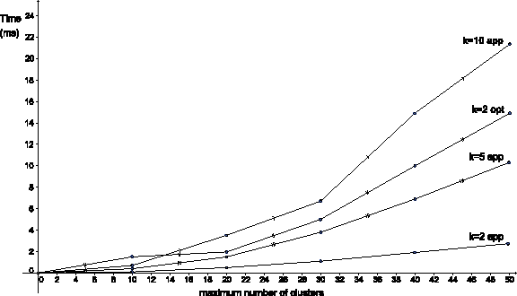
Each performance measurement is obtained to find partition-distance and consensus partition on the simulation set D(λ, 1) and other random partitions. Each point is an average over 100 instances with ± 0.004 SD.

Table 2 shows the performance ratios that are the 2-approximation solution over the optimal solution and the heuristic solution over the optimal solution on the simulation set D(λ, 1) and two random partitions (i.e., k = 3). It is clear that Table 2 shows that the partition-distances of our solutions are at most twice the partition-distances of the optimal solutions.

Table 2.
Each Performance Ratio Is Obtained to Find the Partition-Distance on the Simulation Set D(λ, 1) and Two Random Partitions for the 2-Approximation Algorithm, the Heuristic Algorithm, and the Exact Algorithm When k = 3.

Case Approximation solution Heuristic solution

ρ Optimal solution Optimal solution

10 1.56 1.09

20 1.60 1.22

30 1.61 1.17

40 1.53 1.16

50 1.65 1.21

Each value is an average over 100 instances with ±0.02 SD.

4.2. Simulation test D(λ, 10)

The second data set is settled to simulate possible outcomes of accuracy testing in Butler et al. (2004) and Konovalov et al. (2005a) for a number of clusters, and each cluster contains ten individuals. Hence, we construct the first simulated partition D(λ, 10) which is λ clusters with each cluster containing 10 elements. Other partitions are constructed λ * 10 elements and randomly assign each element to a cluster. The maximum number of clusters of each random partition is less than or equal to λ and the number of elements per cluster is less than or equal to λ. Note that we also do not list the expected time of the exact algorithm of Section 3, since it runs in exponential time in the worst case.

Figure 2 illustrates a few experimental comparisons of expected performance measurements for Gusfield's (2002) algorithm and our approximation algorithm. For example, Konovalov et al. (2005a) reconstructed 5010 individuals from 50 families each containing 10 full siblings. Hence, an instance of the first partition is D(50, 10). In the case, an expected time of our approximation algorithm runs in 16.3ms and Gusfield's (2002) algorithm runs in 36.3ms for k = 2. We also simulate our approximation algorithm for k = 5 and k = 10, respectively. It is also clear that our approximation algorithm runs faster than Gusfield's (2002) algorithm from Figure 2.

FIG 2.
The same as in Figure 1 but for the simulation set D(λ, 10) and other random partitions when k=2, k=5 and k=10. Each value is an average over 100 instances with ±0.005 SD.

Table 3 shows the performance ratios that are the 2-approximation solution over the optimal solution and the heuristic solution over the optimal solution on the simulation set D(λ, 10) and a random partition (i.e., k = 2). It is also clear that Table 3 shows that the partition-distances of our solutions are at most twice the partition-distances of the optimal solutions.

Table 3.
Same as in Table 2 but for the Simulation Set D(λ, 10) and a Random Partition When k = 2

Case* Approximation solution Heuristic solution

ρ Optimal solution Optimal solution

10 1.31 1.23

20 1.24 1.19

30 1.19 1.17

40 1.18 1.15

50 1.17 1.15

Each value is an average over 100 instances with ±0.02 SD.

4.3. Simulation test for k = 3, 4, 5

In this section, we simulate some random data for k = 3, 4, 5. The third data set is settled to simulate possible outcomes for five clusters and each cluster contains five individuals. We construct the first simulated partition D(5, 5) which is 5 clusters with each cluster containing 5 elements. Other partitions are constructed 25 elements and randomly assign each element to a cluster. The maximum number of clusters of each random partition is less than or equal to 5 and the number of elements per cluster is less than or equal to 25.

Table 4 shows the performance ratios that are the 2-approximation solution over the optimal solution and the heuristic solution over the optimal solution on the simulation set D(5, 5) and other random partitions for k = 3, 4, 5. It is also clear that Table 4 shows that the partition-distances of our solutions are at most twice the partition-distances of the optimal solutions.

Table 4.
Each Performance Ratio Is Obtained to Find the Partition-Distance on the Simulation Set D(5, 5) and Several Random Partitions for the 2-Approximation Algorithm, the Heuristic Algorithm, and the Exact Algorithm When k = 3, 4, 5

Case Approximation solution Heuristic solution

K Optimal solution Optimal solution

3 1.24 1.11

4 1.14 1.08

5 1.13 1.07

Each value is an average over 100 instances with ±0.0018 SD.

4.4. Interactive website version

A website to implement Gusfield's (2002) and our algorithms is available at http://mail.tmue.edu.tw/∼yhchen/KPDP.html. We give five input types: (1) user mode, (2) random mode, (3) D(λ, 1) mode, (4) D(λ, 10) mode, and (5) D(λ, any) mode. And we give four algorithms: (a) 2-approximation algorithm, (b) heuristic algorithm, (c) Gusfield's (2002) algorithm (i.e., an exact algorithm for the 2-PD problem), and (d) exact algorithm for k > 2. Before activating the algorithms on the website, you need to fill in the number of partitions (k), the maximum number of clusters of these k partitions (ρ), the maximum number of elements per cluster (N_max), the number of elements (|N|), and select an input type. If you select the user mode, you need to fill in each element to its cluster for each partition P_i, 1 ≤ i ≤ k sequentially. If you choose (3) and (4) modes, all partitions are generated by Sections 4.1 and 4.2, respectively. If you choose (5) mode, you need to fill in each element to its cluster for the first partition P₁, sequentially. Other partitions are randomly generated. After the aforementioned settings, you merely select one algorithm and enter “Run” button to obtain the corresponding solutions to the k-PD problem.

5. Conclusion

In this article, we have shown the first known exact, heuristic, and 2-approximation algorithms for the k-PD problem. It would be interesting and challenging to find a better exact or approximation algorithm for the k-PD problem. Another interesting topic for future research could involve studying whether the 2-PD problem can be exactly solved in O(ρ · |N|) time.

Case	Approximation solution	Heuristic solution
10	1.56	1.09
20	1.60	1.22
30	1.61	1.17
40	1.53	1.16
50	1.65	1.21

Case	Approximation solution	Heuristic solution
10	1.31	1.23
20	1.24	1.19
30	1.19	1.17
40	1.18	1.15
50	1.17	1.15

Case	Approximation solution	Heuristic solution
3	1.24	1.11
4	1.14	1.08
5	1.13	1.07

Footnotes

Acknowledgments

We would like to thank Prof. Shyong Jian Shyu and the anonymous referees, whose useful comments helped to improve this article. This work was supported in part by the National Science Council of the Republic of China under Contract NSC NSC 98-2221-E-133-002.

Disclosure Statement

No competing financial interests exist.

References

Almudevar

, Field

1999. Estimation of single generation sibling relationships based on DNA markers. J. Agric. Biol. Environ. Stat., 4:136–165.

Bagirov

A.M.

, Mardaneh

2006. Modified global k-means algorithm for clustering in gene expression data sets. Proc. ACM 2006 Workshop Intell. Syst. Bioinform., 73:23–28.

Berman

, DasGupta

, Kao

M.-Y.

et al. 2007. On constructing an optimal consensus clustering from multiple clusterings. Inform. Process. Lett., 104:137–145.

Beyer

, May

2003. A graph-theoretic approach to the partition of individuals into full-sib families. Mol. Ecol., 12:2243–2250.

Burkard

, Dell'Amico

, Martello

2009. Assignment Problem. Society for Industrial and Applied Mathematics: New York.

Butler

, Field

, Herbinger

C.M.

et al. 2004. Accuracy, efficiency and robustness of four algorithms allowing full sibship reconstruction from DNA marker data. Mol. Ecol., 13:1589–1600.

Cormen

T.H.

, Leiserson

C.E.

, Rivest

R.L.

et al. 2001. Introduction to Algorithm, 2nd. MIT Press: Cambridge, MA.

Garey

M.R.

, Johnson

D.S.

1979. Computers and Intractability: A Guide to the Theory of NP-Completeness. W.H. Freeman and Company: San Francisco.

Goder

, Filkov

2008. Consensus clustering algorithms: comparison and refinement. Proc. SIAM 9th Workshop Alg. Eng. Exp., 109–117.

10.

Gusfield

2002. Partition-distance: a problem and class of perfect graphs arising in clustering. Inform. Process. Lett., 82:159–164.

11.

Han

, Kamber

2006. Data Mining: Concepts and Techniques, 2nd. Academic Press: San Francisco.

12.

Hirsch

, Swift

, Liu

2007. Optimal search space for clustering gene expression data via consensus. J. Comput. Biol., 14:1327–1341.

13.

Jain

A.K.

, Murty

M.N.

, Flynn

P.J.

1999. Data clustering: a review. ACM Comput. Surv., 31:264–323.

14.

Konovalov

D.A.

2006. Accuracy of four heuristics for the full sibship reconstruction problem in the presence of genotype errors. Proc. 4th Asia-Pacific Bioinform. Conf., 7–16.

15.

Konovalov

D.A.

, Litow

, Bajema

2005a. Partition-distance via the assignment problem. Bioinformatics, 21:2463–2468.

16.

Konovalov

D.A.

, Bajema

, Litow

2005b. Modified simpson O(n³) algorithm for the full sibship reconstruction problem. Bioinformatics, 21:3912–3917.

17.

Konovalov

D.A.

, Manning

, Henshaw

M.T.

2004. KinGroup: a program for pedigree relationship reconstruction and kin group assignments using genetic markers. Mol. Ecol. Notes, 4:779–782.

18.

Kuhn

H.W.

2005. The Hungarian method for the assignment problem. Naval Res. Logis., 52:7–21.

19.

Swift

, Tucker

, Vinciotti

et al. 2004. Consensus clustering and functional interpretation of gene-expression data. Genome Biol., 11:R94.1–R94.16.

20.

Tan

P.-N.

, Steinbach

, Kumar

2006. Introduction to Data Mining. Addison-Wesley: Boston.

21.

Yeung

K.Y.

, Haynor

D.R.

, Ruzz

W.L.

2001. Validating clustering for gene expression data. Bioinformatics, 17:309–318.

22.

, Wong

H.-S.

, Wang

2005. Graph-based consensus clustering for class discovery from gene expression data. Bioinformatics, 21:2463–2468.

Case	Approximation solution	Heuristic solution
ρ	Optimal solution	Optimal solution
10	1.56	1.09
20	1.60	1.22
30	1.61	1.17
40	1.53	1.16
50	1.65	1.21