Reconstructing the History of Large-Scale Genomic Changes: Biological Questions and Computational Challenges

Abstract

In addition to point mutations, larger-scale structural changes (including rearrangements, duplications, insertions, and deletions) are also prevalent between different mammalian genomes. Capturing these large-scale changes is critical to unraveling the history of mammalian evolution in order to better understand the human genome. It also has profound biomedical significance, because many human diseases are associated with structural genomic aberrations. The increasing number of mammalian genomes being sequenced as well as the recent advancement in DNA sequencing technologies are allowing us to identify these structural genomic changes with vastly greater accuracy. However, there are a considerable number of computational challenges related to these problems. In this article, we introduce the ancestral genome reconstruction problem, which enables us to explain the large-scale genomic changes between species in an evolutionary context. The application of these methods to within-species structural variation and disease genome analysis is also discussed. The target audience of this article is advanced undergraduate students in biology.

1. Introduction

The Human Genome Project (HGP) is one of the greatest scientific achievements in the 20th century. In 2001, the draft of the human genome was completed. The human genome has been sequenced in high quality in terms of accuracy and coverage (i.e., the proportion of sequenced bases). One may ask the question: Does this mean that we have almost successfully understood our genomes? Unfortunately, this is not the case. We have only scratched the surface of this question, and we are actually at the very beginning of this long scientific journey; much investigation is still required to understand how genes and the genome contribute to the complex cellular functions of our body.

1.1. Comparative genomics

During evolution, negative (or purifying) selection causes genomic sequences that yield functional products to evolve more slowly than the neutral expectation. Therefore, an important approach to identify the functional sequences in the human genome is to compare it with the genomes of other species and search for conserved regions. Since the Human Genome Project, a number of other mammalian genome sequencing projects have been completed, including mouse, rat, dog, chimpanzee, rhesus macaque, opossum, and cow. The genome sequences from these mammals have greatly advanced the study of mammalian comparative genomics (Miller et al., 2004). Scientists have developed various computational methods to compare these sequenced genomes to select candidate functional regions to further test in the laboratory. The sequencing of more mammalian species is planned.

Besides conserved regions, these mammalian genomes have also provided us a great opportunity to elucidate dramatic genomic differences between species. For example, Figure 1 shows the large-scale chromosomal differences between human and mouse; the sequences in the mouse genome are colored according to their similarity counterparts (or homology) in the human genome. We can observe that a stretch of DNA in human can be scattered into different places in mouse. The figure illustrates about 100 big homologous pieces between human and mouse. In other words, if we cut the human genome into these pieces, we can rearrange them to make a genome similar to that of the mouse genome. We now know that these differences are caused by chromosomal changes that happened some time after the human and mouse diverged (approximately 80 million years ago [MYA]). But can we determine when these changes happened? After human-mouse divergence, did these changes happen on the human lineage or on the mouse lineage?

FIG. 1.

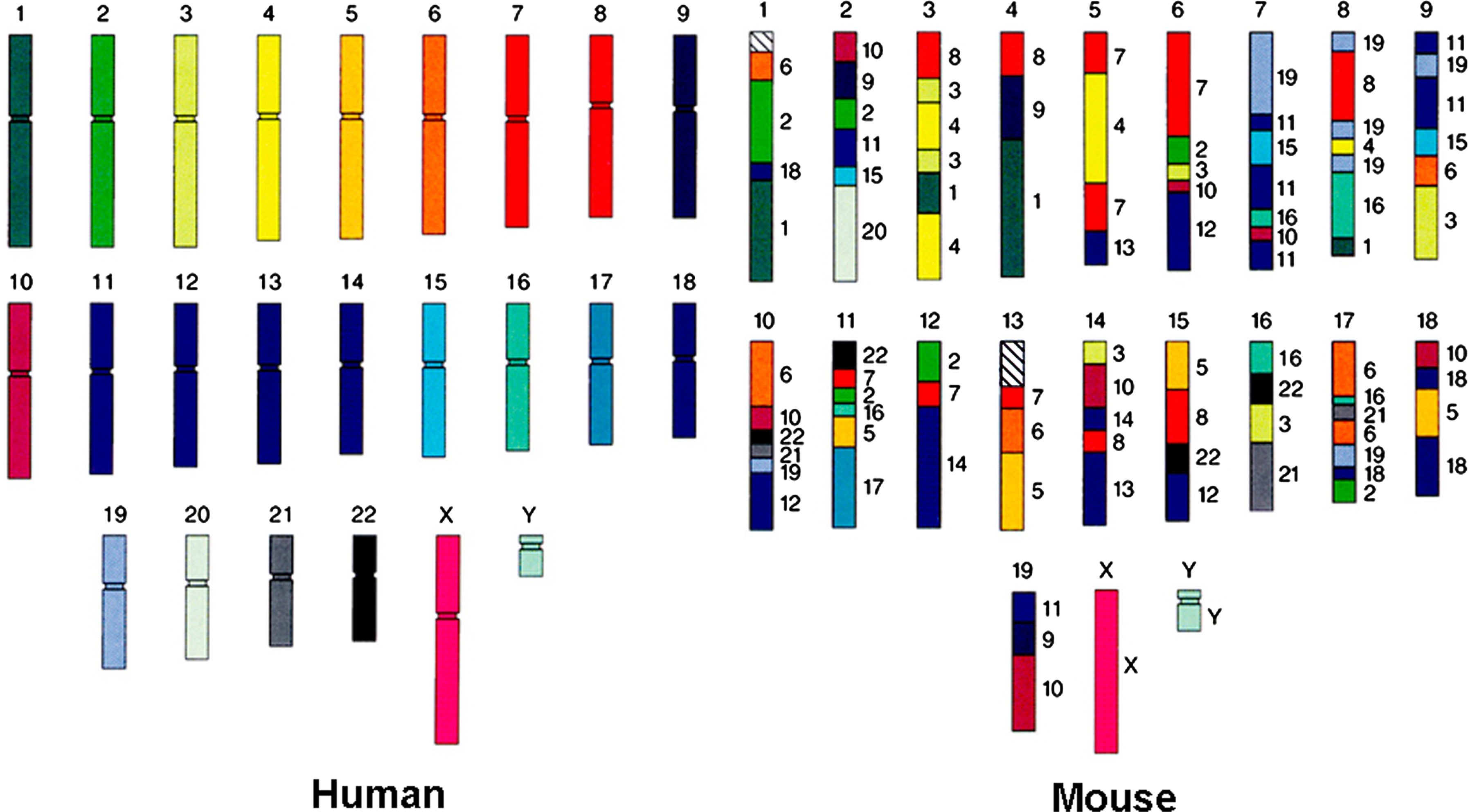
Genomic differences between mouse and human. There are about 100 homologous segments (i.e., the segments in human and mouse share common ancestry) illustrated here. The colors and corresponding numbers next to the mouse chromosomes indicate the human counterparts. Adapted from the original figure, courtesy of Lawrence Livermore National Laboratory.)

In fact, if we compare only the human and mouse genomes, we cannot answer this question. Since both human and mouse evolved from a common ancestor, more species are needed to determine when the genomic rearrangements happened after human and mouse diverged. Figure 2 illustrates mammalian evolution. The phylogenetic tree shows the evolutionary relationships between human and some representative mammalian species, from the closest relative chimpanzee (divergence time 4–5 MYA), to platypus, which shares a mammalian common ancestor with human at approximately 160 MYA. We are particularly interested in the changes in molecular evolution along the branch toward modern human, because those genomic innovations may greatly contribute to distinguishing human from other mammalian species. Hence, systematic comparative genomic analysis will shed light on one of the most exciting questions in science: How did we become human?

FIG. 2.

The phylogeny of mammalian species. Figure is modified from Figure 1 in Margulies et al. (2007) with the relationship among Boreoeutheria, Xenarthra, and Afrotheria adjusted based on Murphy et al. (2007).

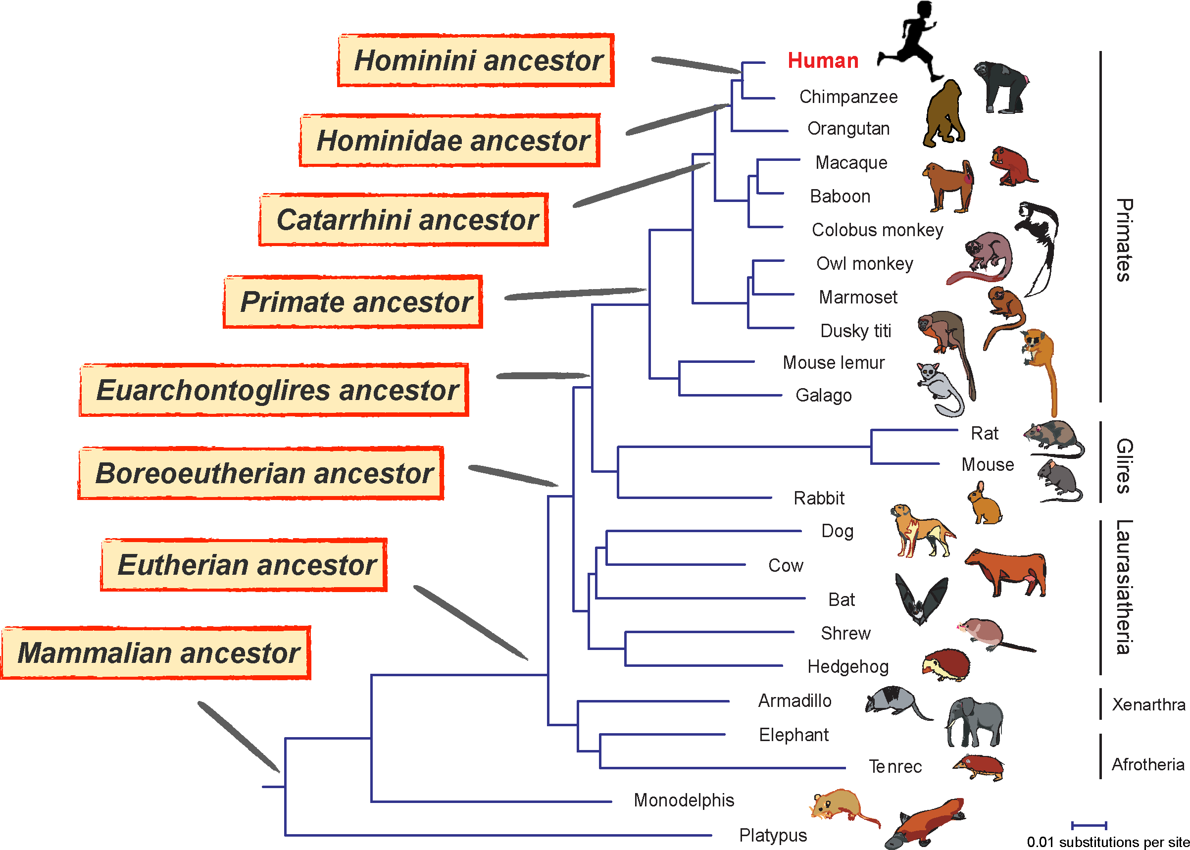
We know that the differences between mammalian genomes in Figure 2 are the result of evolutionary changes after their divergence from their common ancestor. For example, all placental mammals share a common ancestor, called the Boreoeutherian common ancestor. Over the last 100 million years, that ancestor's descendants have evolved into a complex array of different placental mammals—of which, about 5,000 are currently living on the planet. As the result of speciation events and many significant changes in each lineage, we see remarkable differences among living placental mammals, both genetic and morphological. If we could somehow obtain the genome of those ancestral species at the precise moment of speciation for each branch in the phylogenetic tree in Figure 2, we would be able to compare two genomes on both sides (one ancestor and one descendant) and determine exactly what happened during a particular period of time in mammalian evolution. That would be incredibly exciting, since this unravelled trajectory would tell us how the human genome reached its present state of evolution. Sadly, although new technologies allow us to get DNA from specimens of some relatively recent ancient species, for example, Neanderthal (Green et al., 2006) and woolly mammoth (Miller et al., 2008), we cannot directly obtain DNA sequences older than a million years. However, the mammalian genomes already sequenced and the additional diverse set of mammalian species that will be sequenced in the future give us an alternative approach.

1.2. Genome reconstruction provides an additional dimension for comparative genomics

All placental mammals living today show a wide range of variation. However, since these species are descended from a common ancestor, they all have inherited specific DNA sequences from the ancestral genome. Therefore, given the genomes of related species, we can use computational analysis to work backwards and determine most of the specific DNA changes that probably occurred, reconstructing the history of the genetic changes for all the individual bases. With the reconstructed history, we will be able to explain the genomic changes on any given lineage, including the human lineage. This will provide an extremely illuminating vertical map, in the sense that we can view the evolutionary changes from past to present directly, decoding the molecular basis for the extraordinary diversity of mammalian forms and capabilities.

Here, we use two examples to show that genome reconstruction can provide an additional dimension for comparative genomics analysis and facilitate discoveries. Figure 3 shows a gene called acyltransferase 3 (ACYL3), which was present in archaea, bacteria, and eukaryotes. ACYL3 is still found in the genomes of many mammals, such as rhesus, rat, mouse, and dog, but has been lost in both human and chimpanzee (Zhu et al., 2007). What happened? Figure 3 illustrates the reconstructed history of this gene, which gives us a direct sense of what transpired from past to present. A close look reveals that there was a G to A transition that happened after the primate common ancestor and before the ape common ancestor. This nonsense mutation changed the tryptophan codon (W) to a stop codon and made this gene non-functional.

FIG. 3.

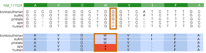
Part of the reconstructed history of the ACYL3 gene (NM_177028), which was lost in both human and chimpanzee. Boreoeutherian, the reconstructed sequence in the Boreoeutherian ancestor; euArc, the Euarchontoglires ancestor; primate, the primate common ancestor; ape, the human-chimpanzee common ancestor. The G to A transition is highlighted in the DNA multiple sequence alignment (top). The consequence, a change from a tryptophan codon (W) to a stop codon, is also illustrated in the alignment with codon translation (bottom).

The second example is a region called Human Accelerated Region 1 (HAR1) (Pollard et al., 2006) with 118 base pairs. Almost all the bases are conserved in mammalian species; furthermore, only two bases differ between chimpanzee and chicken (310-MY divergence time). However, human has surprisingly accumulated 18 substitutions since human and chimpanzee divergence. Figure 4 shows the reconstructed history of part of the HAR1 region, highlighting 11 out of the 18 substitutions. Scientists believe that this region has experienced accelerated evolution in the human genome due to positive selection. It turns out that HAR1 is part of a novel RNA gene that is expressed specifically during a critical window in embryonic development for a specific set of neurons that guide the development of the layers of the cerebral cortex.

FIG. 4.

Part of the reconstructed history of the Human Accelerated Region 1 (HAR1). Mutations that accumulated in human after diverging from the chimpanzee common ancestor are highlighted.

The above examples have demonstrated that, if we can create such a reconstructed evolutionary history, we will be able to make a lot of discoveries like this, which will be enormously exciting for human biology. But what kind of computational methods should we use to create such a vertical map that documents all the important genomic changes in mammalian evolution?

1.3. Base-level ancestral reconstruction

In addition to point mutations, which are the most common small-scale genomic changes, various other types of genomic changes can occur. In multiple alignment for sequences from different species, we often see gaps in some of the sequences. What do those gaps mean? Let's examine the following example:

human	ATCAGC------GGCGAT
chimp	ATCAGC------GGCGAT
macaque	ATCAGCCGGATCGGCGAT
mouse	ATCAGCCGGATCGGCGAT
rat	ATCAGCCGGATCGGCGAT
dog	ATCAGCCGGATCGGCGAT
cow	ATCAGCCGGATCGGCGAT

Actually, the gaps in the alignment correspond to insertion and deletion (indel) events. In the above example, we can infer that the gaps in human and chimpanzee reflect a deletion event that happened before human-chimp common ancestor but after human-macaque common ancestor, which by the principle of parsimony is more likely than any other scenarios. Determining the most plausible indel scenario is the basic idea of inferring indel events from the multiple alignment.

Note that the quality of multiple alignment is critically important for base level reconstruction. The reconstruction methods usually assume that the alignments are evolutionarily correct: in other words, all the bases are placed in the same alignment column as long as they are derived from the same ancestral base, and the boundaries of gaps are placed perfectly consistently with the indel events. Unfortunately, perfect alignment is in practice hard to achieve, especially for genomic regions that have repeatedly undergone various types of genomic changes. The good news is that the majority of the mammalian genomes can be aligned with high confidence. Blanchette et al. (2004) showed that, given a large genomic region in which there has been no shuffling of bases since the most recent common ancestor, the Boreoeutherian ancestral sequence can be recovered with an accuracy as high as 98% from only 20 optimally chosen modern mammals. Now, how can we reconstruct the entire ancestral genome? The challenge remains: for whole-genome analysis, we must consider large scale chromosomal changes between different species.

2. Cross-Species Large-Scale Genomic Changes

2.1. Genome rearrangements

A chromosome is a threadlike macromolecular complex. In eukaryotic cells, chromosomes have a linear form rather than circular. Each chromosome has two arms; the shorter one is called the p arm, while the longer one is the q arm. A chromatid is one of the two identical parts of the chromosome after the synthesis phase. Two chromatids are attached at an area called the centromere. The telomere is the region found at either end of a linear chromosome.

Different kinds of organisms have different numbers of chromosomes. For example, humans have 23 pairs of chromosomes, dogs have 39 pairs, and mice have 20 pairs. A graphic representation of all the chromosomes in a cell of any species is called a karyotype. Karyotype diversity among different species is caused by chromosome rearrangements. Dobzhansky and Sturtevant (1938) reported the observation of inversion events between two Drosophila species, thus pioneering the study of chromosome rearrangement. Since then, many studies have concentrated on understanding the differences between genome architectures from an evolutionary perspective. These rearrangements are genomic “earthquakes” (Alekseyev and Pevzner, 2007) that change the chromosomal architecture of an organism. We know that there are a number of different types of rearrangement operations that can be accumulated during chromosomal evolution. In general, these rearrangements are comprised of inversions, translocations, fusions, and fissions.

Figure 5 illustrates these four rearrangement operations. In an inversion operation, a genomic segment on one chromosome is reversed and complemented (e.g., AAGTCAT becomes ATGACTT). In a translocation operation, the end part of one chromosome is swapped with the end of another chromosome. In a a fusion operation, two chromosomes are joined to form one chromosome; while in a fission operation, a single chromosome is broken into two chromosomes. Among these operations, inversions are the most common events in chromosomal evolution. For translocations, there are two main types, reciprocal (Fig. 5C) and Robertsonian. A Robertsonian translocation involves two chromosomes, in which their long arms fuse at the centromere and the remaining two short arms are lost. It has been suggested that Robertsonian translocation also occurred in mammalian genome evolution.

FIG. 5.

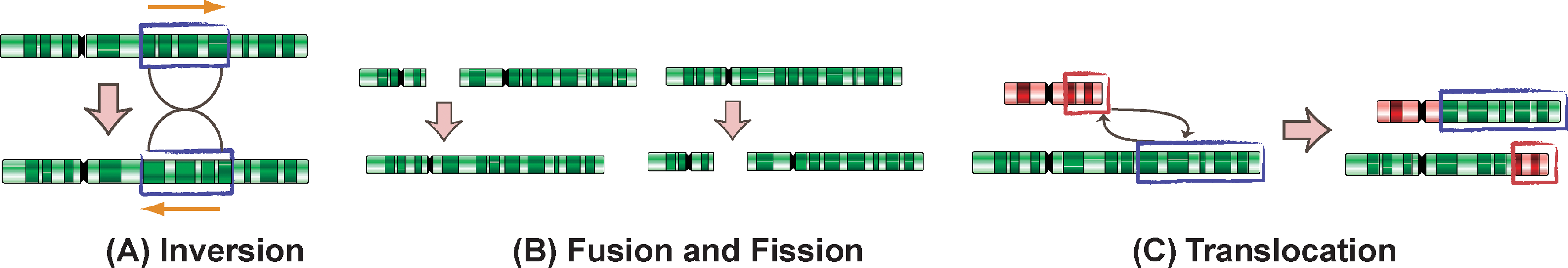
Different types of genomic rearrangements. Each green or red rectangle is a chromosome. Each big arrow indicates what the chromosomes look like before and after the rearrangement operation.

In the general mathematical model of chromosome evolution, a chromosome can be represented as a string of signed numbers (or signed permutation), and a genome as a set of these strings, for example, 1 2 3 4 5 • 6 7 8, where • separates chromosomes. Numbers could represent any genomic content, for example, a single base, a gene, or a longer DNA sequence. Numbers have signs, either + or −, which indicate the relative orientation of the genomic content.

Here are some examples of chromosome rearrangements within this mathematical structure:

Inversion: 1 2 3 4 5 • 6 7 ⇒ 1 −4 −3 −2 5 • 6 7 (in bioinformatics literature, inversion is also called reversal);

Translocation: 1 2 3 4 5 • 6 7 ⇒ 1 7 • 6 2 3 4 5;

Fusion: 1 2 3 4 5 • 6 7 ⇒ 1 2 3 4 5 6 7;

Fission: 1 2 3 4 5 • 6 7 ⇒ 1 2 • 3 4 5 • 6 7.

Overlapping or nested operations form composite operations. For example, 1 2 3 4 5 6 7 can be transformed to 1 −4 −6 • −5 2 3 7 by two overlapping inversions followed by a fission: 1 2 3 4 5 6 7 ⇒1 −4 −3−2 5 6 7 ⇒ 1 −4 −6 −5 2 3 7 ⇒ 1 −4 −6 • −5 2 3 7.

2.2. Synteny blocks

Identifying the genomic content that signed permutations can represent has always been an essential problem in studying genome rearrangements. Nadeau and Taylor (1984) first introduced the term “conserved segment” to name a maximal genomic segment with preserved gene orders that are not disrupted by rearrangements between species. In the past decade, using comparative gene mapping to find orthologous gene loci as the evolutionary markers played an important role in testing algorithms and understanding rearrangement scenarios (the term “orthologous” means that two loci share the same ancestry). However, although this approach works well in small genomes, for example, virus genomes or mitochondrial genomes, reliable gene annotation and orthology assignment in the entire mammalian genome are technically very difficult, partly because of the great number of duplicated genes existing in mammals. This problem is further complicated by the large proportion of non-coding regions throughout the genome.

Pevzner and Tesler (2003) proposed the GRIMM-Synteny algorithm to partition the genomes into segments that tolerate a certain amount of local microrearrangements that are smaller than the size of the segments. These segments are called “synteny blocks,” which conceptually is similar to conserved segments. Based on this method, multi-way synteny blocks can be created for multiple species. The GRIMM-Synteny algorithm greatly improved the resolution and precision for whole-genome rearrangement studies.

In recent years, improved whole-genome alignments have allowed us to produce synteny blocks with higher coverage and higher resolution for ancestral genome reconstruction. Ma et al. (2006) is one of these methods. The basic idea can be summarized in Figure 6. If two synteny blocks are adjacent in one species and separate in the other, which reflects a breakpoint between these two species. The algorithm processes the whole-genome alignment and partitions the genome every time it encounters a breakpoint in one of the species. In the example in Figure 6, if we set the synteny block threshold as 50kb (i.e., any rearrangements smaller than 50kb are ignored), this region can be partitioned into five synteny blocks.

FIG. 6.

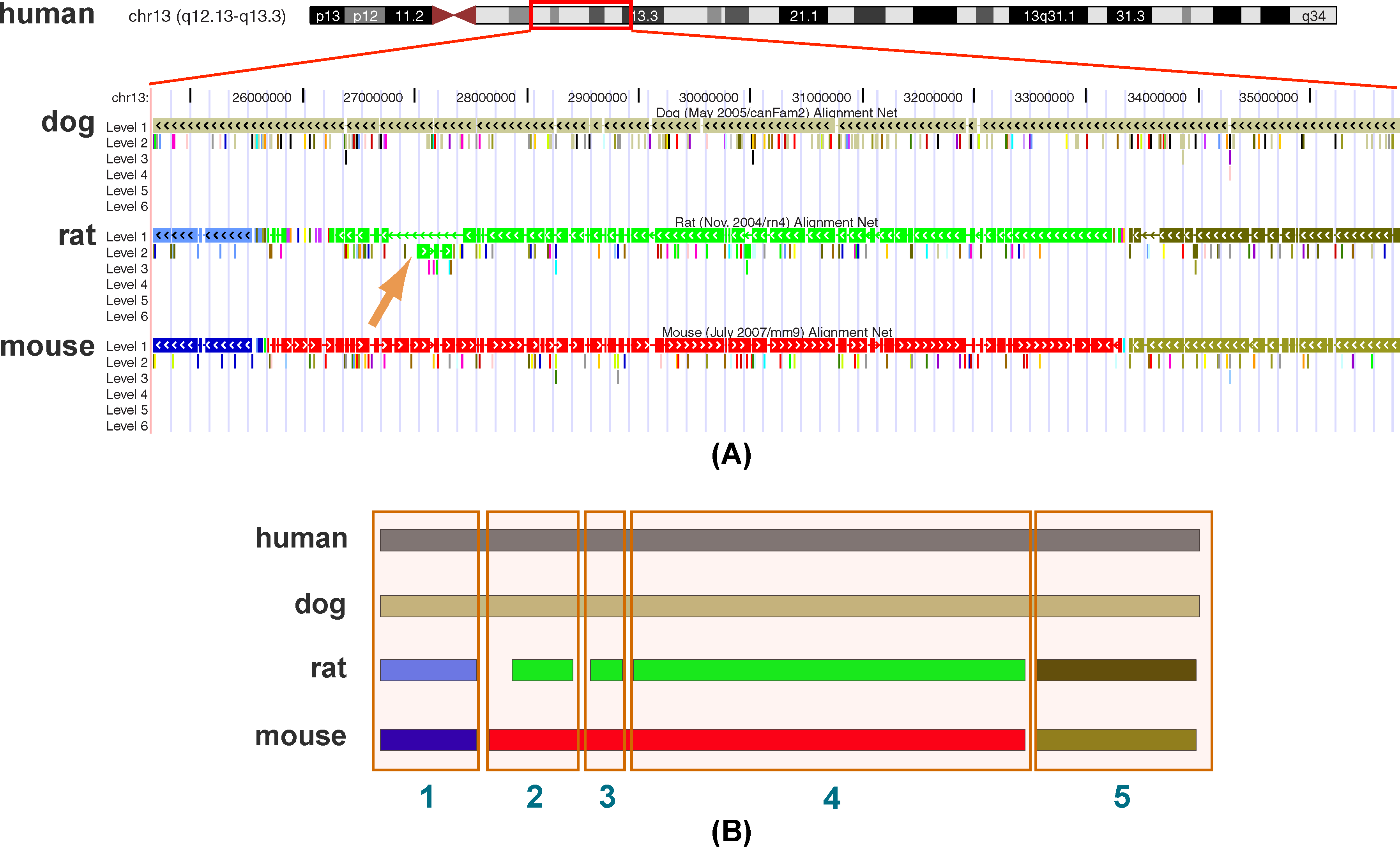
Constructing synteny blocks based on whole-genome alignment. (A) A region on human chromosome 13 and its corresponding regions in mouse, rat, and dog (based on their pairwise alignments with human). Different colors refer to different chromosomes in dog, rat, and mouse. This is a snapshot of the UCSC genome browser for this region on human chromosome 13. Each track is a pairwise alignment net between human and a secondary species. In the figure, net identifies putative orthologous genomic segments between two genomes. Level 1 net shows the primary alignment of the region. For example, this human region is roughly orthologous to three regions in different chromosomes in mouse (shown by three colors). Level 2 and beyond show additional nets, which indicate rearrangements (smaller than level 1). For example, the orthologous region on rat chromosome 12 (the green part) has a big net as a level 2 net (indicated by an orange arrow), suggesting a rearrangement. (B) An abstract version of (A), where this genomic region can be partitioned into five synteny blocks.

When we construct synteny blocks, resolution (size threshold) is always a factor to consider (low resolution = large blocks and high resolution = small blocks). If we construct higher resolution synteny blocks, we can capture more interesting rearrangements, but the smaller ones may not be very reliable due to potentially problematic sequence alignment. If we build lower resolution synteny blocks, we will have more reliable evolutionary conserved synteny blocks, but we certainly miss a lot of rearrangements that are under the size threshold. In Ma et al. (2006), for human, mouse, rat, and dog, 1338 synteny blocks (size threshold = 50kb) were constructed, covering about 95% of the human genome.

Once we have the synteny blocks, the next step is to figure out what the ancestral order and orientation of these blocks were in a certain ancestor and what kinds of evolutionary events caused the dramatic shuffling of these blocks in different descendant species.

2.3. Duplications and other structural changes

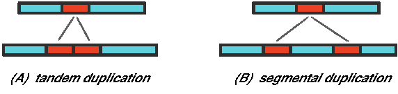
Besides the rearrangement operations mentioned above, chromosome architecture can also be changed by other large-scale operations. For example, transposition is a more complicated rearrangement in which a segment of DNA is removed from its original location and then gets inserted into a new location. Duplication is another major source of large scale genomic change. There are generally two types of duplication events: tandem duplication and segmental duplication (Fig. 7). In addition, large-scale insertion and deletion can also happen. Even more complex operations are occasionally observed in human disease-associated genome rearrangements (Lee et al., 2007).

FIG. 7.

(A) Tandem duplication, where the two copies are adjacent to each other after the duplication. (B) Segmental duplication, where the target copy is far away from the source copy after the duplication.

All these operations may happen in nested or overlapping forms during evolution. As a result, genomic architectures between different modern species can be highly distinct. An ancestral genomic segment can be broken into several fragments in an extant genome and widely scattered to different chromosomes and different positions (Fig. 1).

3. Reconstructing Evolutionary History

3.1. Ancestral karyotype reconstruction

In fact, the problem of ancestral mammalian karyotype reconstruction has been studied for quite a long time. The development of comparative gene mapping and cytogenetic methods have provided biologists with powerful tools in their attempt to solve the puzzle. However, the number of chromosomes in the mammalian common ancestor is still not fixed and is believed that 24 or 25 is currently the best guess. Even though there is no solid evidence of the number of chromosomes in the ancestral eutherian karyotype, some configurations have been widely confirmed, for example, Hsa14/Hsa15 (“Hsa” refers to a human chromosome), which means human chromosomes 14 and 15 were in the same ancestral chromosome (in other words, a chromosomal fission happened on the path leading to human).

In the past decade, the primary experimental technique used in the study of chromosomal evolution is chromosome painting, in which fluorescently labeled chromosomes from one species are hybridized to chromosomes from another species so that breakpoints can be identified. Although the requirement of optical visibility means that the chromosome painting approach can recognize only rearrangements with long conserved segments and cannot identify intrachromosomal rearrangements, the chromosomal painting approach has the advantage that data are available for more species because we don't need to sequence the genome.

3.2. Rearrangement-based ancestral reconstruction

Indeed, for the past 15 years, genome rearrangement problems have fascinated computational biologists. Computer scientists have also tried to reconstruct the ancestral genome architecture using bioinformatic algorithms in a parsimony framework based on certain distance measurements.

Sankoff et al. (1992) pioneered the theoretical study of reversal distance, and phylogenetic analysis using gene order data. The analysis of the most parsimonious rearrangement scenarios is the central part of theoretical genome rearrangement study, among which the most well studied is sorting by reversals. Sorting by reversals is the problem of converting one permutation into another using the minimum number of reversal operations. The minimal number of reversals is regarded as reversal distance between two permutations. For example, in Figure 8i, the reversal distance between A and B, abbreviated d(A, B), is 7 because 7 is the minimum number of inversions needed to transform A into B. For these kind of signed permutations, which are very important to model mammalian genomes, Hannenhalli and Pevzner (1995) gave the first efficient algorithm to solve the sorting by reversal problem.

FIG. 8.

(i) One most parsimonious solution of sorting by reversal between A and B. (ii) An example of the Median Problem. The median M = 1 2 3 −4 −5 6 −8 −7, with d(A, M) + d(B, M) + d(C, M) = 8.

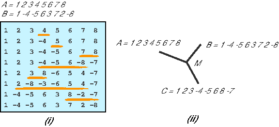
However, when we need to use reversal distance to perform phylogenetic analysis (in which we need more than two species), the problem suddenly becomes computationally intractable. A typical problem is the Median Problem: Given three signed genomes A, B, and C, as well as the distance measure d, find a median genome, which is a genome M such that Σ d = d(A, M) + d(B, M) + d(C, M) is minimal, as illustrated in Figure 8ii. Unfortunately, this problem is computationally intractable. Note that the Median Problem is the simplest problem for genome reconstruction problem based on reversal distance, in which we have two descendant genomes A and B as well as an outgroup species C. However, there are heuristic approaches available to solve this problem, for example, MGR (Bourque and Pevzner, 2002).

3.3. Adjacency-based ancestral reconstruction

Two synteny blocks are adjacent if they are next to each other on a chromosome. Ma et al. (2006) observed that the adjacencies of genomic content in modern species can be used to infer the ancestral adjacencies. The problem can be described as follows: given a tree, predict the ancestral order and orientation based on adjacencies in modern genomes. That is, consider the end of a synteny block x that does not correspond to a human telomere or centromere. How can we identify the segment that was adjacent to x in the ancestral genome?

If the segment that is currently adjacent in human is identical to the one that is adjacent in dog (but a different segment is adjacent in mouse and rat), the most parsimonious assumption (based on the phylogeny of human, mouse, rat, and dog, as shown in Fig. 9) is that the first and second segments were adjacent in the ancestral genome (and that a disruption occurred in the rodent lineage at this genomic position).

FIG. 9.

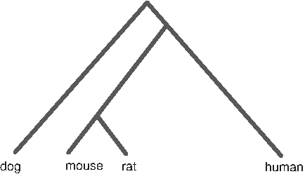
The phylogeny of human, mouse, rat, and dog.

If the same segment is adjacent to the chosen segment in human, mouse, and rat, but not in dog, we need more information to confidently predict the ancestral configuration, since there is a chance that the dog adjacency is ancestral and that the breakage occurred on the short branch from the human-dog ancestor to the human-rodent ancestor. To help resolve these cases, we can add outgroup information, for example, the opossum sequence. Figure 10 shows an example that demonstrates this principle. This snapshot from the UCSC genome browser clearly shows the relative orientations from which the ancestral orientation can be inferred by parsimony. This region can be partitioned into three synteny blocks: 1, 2, and 3. Human, rhesus, mouse, and rat share the order 1 2 3, while dog and opossum have the order 1 − 2 3. Based on the parsimony principle discussed above, we can infer that 1 is followed by −2 and 3 is preceded by −2 in the human-dog common ancestor, which creates the ancestor order 1 −2 3. How can we generalize this procedure algorithmically?

FIG. 10.

(A) The phylogenetic tree of human, rhesus, mouse, rat, dog, and opossum, where opossum is an outgroup of the placental mammals (all the descendants of the Boreoeutherian common ancestor). (B) A snapshot of the UCSC genome browser of this region. Each track is a pairwise alignment net between human and a secondary species. In this region, both dog and opossum have level 2 net that reflects an inversion in the alignment with human. Based on the tree in (A), we infer that the inversion happened on the branch leading from the Boreoeutherian common ancestor to the Euarchontoglires common ancestor (the primate-rodent ancestor), as highlighted by the orange arrow. The corresponding human region is hg18.chr13:57,380,591-57,383,765.

The approach is inspired by the method of Fitch (1971), which was originally used to infer minimum substitutions in a specified tree topology. For that problem, one is given a phylogenetic tree and a letter for every position in each leaf of the tree (corresponding to the contents of orthologous sequence sites). The problem is to infer the ancestral letters (corresponding to internal nodes of the tree), so as to minimize the number of substitutions (i.e., differences between the letters at each end of an edge in the tree).

The algorithm works sequentially, in two stages. For each position, in a bottom-up fashion, it first determines a set M_π of candidate nucleotides at each node π in the tree according to the following rule: if π is a leaf, M_π just contains its nucleotide character; otherwise, if π has children τ and φ, then M_π equals either to intersection M_τ ∩ M_φ or the union M_τ ∪ M_φ depending on whether M_τ and M_φ are disjoint or not. That is,

if M_τ and M_φ do not overlap

then M_π ← M_τ ∪ M_φ

else M_π ← M_τ ∩ M_φ

Then, in a top-down fashion, it assigns a character b_π from M_π to π according to the following rule: Let ρ be the parent of π; if the character b_ρ assigned to ρ belongs to M_π, then, b_π = b_ρ. Otherwise, set b_π to be any character in M_π. Although character assignment in this second stage may not be unique, any assignment gives an evolutionary history with the minimum number of substitution events.

The rationale behind Fitch's method is as follows. If the character b_π belongs to both children of π, then an optimal strategy for labeling nodes in the subtree rooted at π is to put b at each of π, τ and φ, and label the subtrees of τ and φ optimally. If there is no such b, then the strategy is to put a character from either M_τ or M_φ at π, pay for one substitution to reach the other child, and optimally label the two subtrees (Fig. 11). The characters at leaves are given. Then we do a postorder tree traversal (i.e., visiting each node in the tree by recursively processing all subtrees and finally processing the root) and create sets in the internal nodes until we reach the root. In this example, the ancestral nucleotide A will give us the minimum number of substitutions, which is 2, for this position.

FIG. 11.

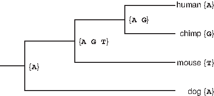
An example of Fitch's algorithm.

Let's now formally prove by induction that the Fitch algorithm constructs the most parsimonious solution for the total number of substations. Let k(π) denote the minimum number of substitutions in the subtree rooted at π. Let τ and φ be the two children of π. Basis: if tree height h = 1, then τ and φ are leaves in the phylogeny. If τ and φ are the same, then no substitution is needed; k(π) = 0. Otherwise, only 1 substitution is needed; k(π) = 1. Induction: we assume the Fitch algorithm constructs the most parsimonious solution for the subtree height is h, then prove this is the case for height h + 1. If the intersection of M_τ and M_φ is not empty, then we can have k(π) = k(τ) + k(φ) by assigning any character in the intersection to π. Otherwise, k(π) is k(τ) + k(φ) + 1, by assigning any character in the union of M_τ and M_φ. This completes the proof.

In our case, we deal with sequences of signed integers, rather than characters of nucleotides or amino acids, and instead of keeping track of letters at a particular sequence position, we track the synteny blocks for each of the immediately adjacent positions. Based on this logic, for a certain ancestor, we can infer what would be the most parsimonious neighbors of each synteny block in the ancestral genome.

We first define predecessor and successor. If modern genome g contains synteny block i, then the predecessor p_g(i) is defined as the signed block that immediately precedes i on the same chromosome relative to the original orientation. In the opposite orientation, p_g(−i) immediately precedes − i in the reverse complement of the same chromosome. We set p_g(i) = φ if i appears first on a chromosome. The successor s_g(i) of i is defined analogously; we set s_g(i) = φ if i appears last on a chromosome. For instance, let g have the chromosome (1 − 4 − 3 5 2). Then, in the positive orientation, we have: p_g(1) = 0, p_g(2) = 5, p_g(−3) = −4, p_g(−4) = 1, p_g(5) = −3, while s_g(1) = −4, s_g(2) = 0, s_g(−3) = 5, s_g(−4) = −3, s_g(5) = 2. In the opposite orientation, (−2 −5 3 4 −1), we have: p_g(−1) = 4, p_g(−2) = 0, p_g(3) = −5, p_g(4) = 3, p_g(−5) = −2, while s_g(−1) = 0, s_g(−2) = −5, s_g(3) = 4, s_g(4) = −1, s_g(−5) = 3.

We consider keeping track of the set of all possible synteny blocks that follow a fixed synteny block in a most-parsimonious evolutionary scenario. In the genome that corresponds to node π, block i could be followed by any block that follows i in both τ and φ, without requiring any rearrangements on the branches leading from π to its children. Otherwise, i can be followed by any block that follows i in one of π's children, at the cost of a chromosomal break next to i along the branch leading from π to the other child. This is all closely analogous to the case of substitutions, as sketched above.

Thus, for any genome g, we associate with each block i two sets of signed blocks, denoted P_g(i) and S_g(i), giving potential predecessors and successors of i relative to chromosomes of g. If g is a modern genome, P_g(i) = {p_g(i)} and S_g(i) = {s_g(i)}, for each i. If g does not contain i, then both sets are empty.

Algorithm 1, Get-Predecessor-Successor(R), constructs P_g(i) and S_g(i) for each synteny block i of every ancestral genome g in the tree (π is a tree node; τ and φ are π's children in the tree; N is the total number of synteny blocks):

Algorithm 1 Get-Predecessor-Successor (π)
1	if π is non-leaf node
2	then Get-Predecessor-Successor(τ)
3	Get-Predecessor-Successor(φ)
4	for i ← −N to N (i ≠ 0)
5	do if P_τ(i) and P_φ(i) do not overlap
6	then P_π(i) ← P_τ(i) ∪ P_φ(i)
7	else P_π(i) ← P_τ(i) ∩ P_φ(i)
8	if S_τ(i) and S_φ(i) do not overlap
9	then S_π(i) ← S_τ(i) ∪ S_φ(i)
10	else S_π(i) ← S_τ(i) ∩ S_φ(i)

Finally, there is an algorithm to connect the synteny blocks in the ancestor based on possible predecessor/successor relationships into continuous ancestral regions (CARs), which resemble ancestral chromosomes. Using 1338 synteny blocks constructed from human, mouse, rat, and dog, the karyotype of the Boreoeutherian ancestral genome (Fig. 12) can be reconstructed with relatively high accuracy (Ma et al., 2006; Rocchi et al., 2006). The accuracy can be assessed by comparing to experimental chromosomal painting results and computational simulations.

FIG. 12.

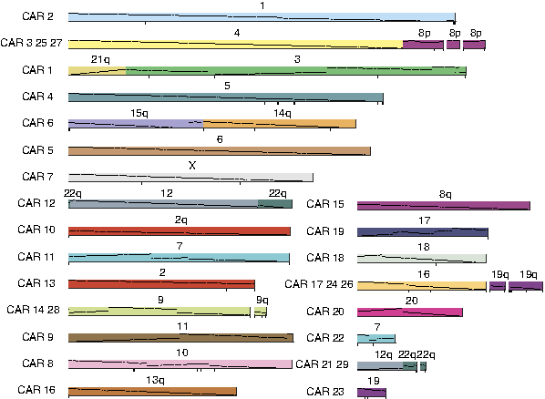
Map of the Boreoeutherian ancestral genome. Numbers above bars indicate the corresponding human chromosomes. 1338 synteny blocks are constructed from whole genome sequences of human, mouse, rat, and dog (size threshold = 50kb; covering about 95% of the human genome).

3.4. Challenges and future directions

The method discussed in the previous section, which was based on adjacencies of synteny blocks, reduced the number of discrepancies between computational and experimental large-scale genome reconstruction. The result, in much higher resolution than previous studies, has proven to be reliable (Rocchi et al., 2006). However, such an adjacency-based reconstruction, albeit undoubtedly informative, provides no direct knowledge of the detailed evolutionary operations transforming the ancestor to the present day genomes. Therefore, models that handle sophisticated genomic operations are needed.

With regard to models of evolutionary operations, a key step was the unification of inversion, translocation, fusion, and fission into the general operation of double-cut-and-join (DCJ) (Yancopoulos et al., 2005) (also termed “two-break operation”; Fig. 13). Other types of operation were also studied (e.g., transposition and indels). More importantly, duplications cannot be left out of the analysis given their critical role in mammalian evolution. Regarding recovering complex operations on genomes, a recent article by Ma et al. (2008) formalized the problem of recovering (by parsimony) the evolutionary history of a set of genomes that are related to an unseen common ancestor genome by operations of deletion, insertion, duplication, and rearrangement of segments of bases, and by speciation events. The authors show that, as the number of bases (“sites”) in the genome approaches infinity, the problem of reconstructing simplest history of operations becomes tractable.

FIG. 13.

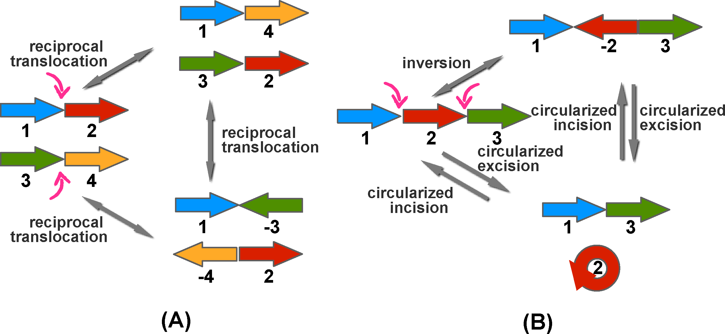
Two-break operations, in which we break the genome in two places, creating four free ends, and then we rejoin the four free ends. (A) Two breakpoints are on the different chromosomes; this models translocation. (B) Two breakpoints are on the same chromosome; this models inversion and indels.

There are a number of computational challenges ahead. For example, so far most algorithms assume that each operation is equally likely to happen in the genome. To be more realistic, each of the different types of operations could have a different cost, and the goal would be to find an evolutionary history with minimal total cost. This method is called weighted parsimony. Models that consider weighted parsimony based on empirical data from practice will be very useful.

In addition, breakpoint reuse, in which the same genomic location is broken more than once during evolution, arises in real data, partly because the synteny block construction method often cannot pinpoint the breakpoint to one-base resolution. It is also still a challenge to locate more precise breakpoints caused by structural changes, widely believed to contain enriched genomic variation and very interesting biology (Larkin et al., 2009).

4. Chromosomal Aberrations in Human Disease Genomes

Many individual human genomes have been entirely sequenced, including the Nobel Laureate James Watson, a Han Chinese individual, a Korean individual, and Yoruban individuals. These data revealed that, between different normal human individuals, our genomes also show a large amount of structural variation. One may wonder: How representative is the reference human genome sequenced by the Human Genome Project a decade ago?

We now know that many human diseases are associated with structural genomic changes. New technologies are allowing researchers to map disease-causing structural changes to the genome in much finer resolution. When multiple changes have occurred to the genome and created a genetic state that causes diseases, the algorithms of genome reconstruction discussed above may be useful in better understanding the detailed scenario of these changes, as well as identifying the specific operations that have occurred and the properties of the DNA sequences near their breakpoints.

Cancer is another group of genetic diseases associated with a massive amount of structural genomic changes. Much as germline genomes undergo various chromosomal structural changes over an evolutionary timescale, genomes of somatic cells also undergo structural changes during cancer progression, including rearrangements, insertions and deletions, and duplications. Recent rapid advancement in high-throughput sequencing technologies have enabled us to use paired-end reads to map novel DNA segment adjacencies caused by different types of rearrangements in individual tumor genomes. A paired-end read consists of two stretches of sequenced DNA with an unsequenced insert of known size between them. Thus, after mapping the paired-end read from a tumor genome to a normal genome, if the distance between those two stretches of DNA changes, then we know there must be a structural genomic change. Interested readers can read Medvedev et al. (2009) for computational approaches to utilize paired-end data.

Figure 14A shows a CACNA2D4-WDR43 fusion gene in NCI-H2171, a lung cancer cell line (Campbell et al., 2008). Figure 14B shows a ETV6-ITPR2 fusion gene generated by a 15-Mb inversion in breast cancer sample PD3668a (Stephens et al., 2009). Stephens et al. (2009) reported rearrangement patterns in 24 breast cancer genomes. With these cancer breakpoint data coming in, the rearrangement-based algorithms may help us better dissect the evolutionary history of individual tumors and understand molecular signatures of different cancers.

FIG. 14.

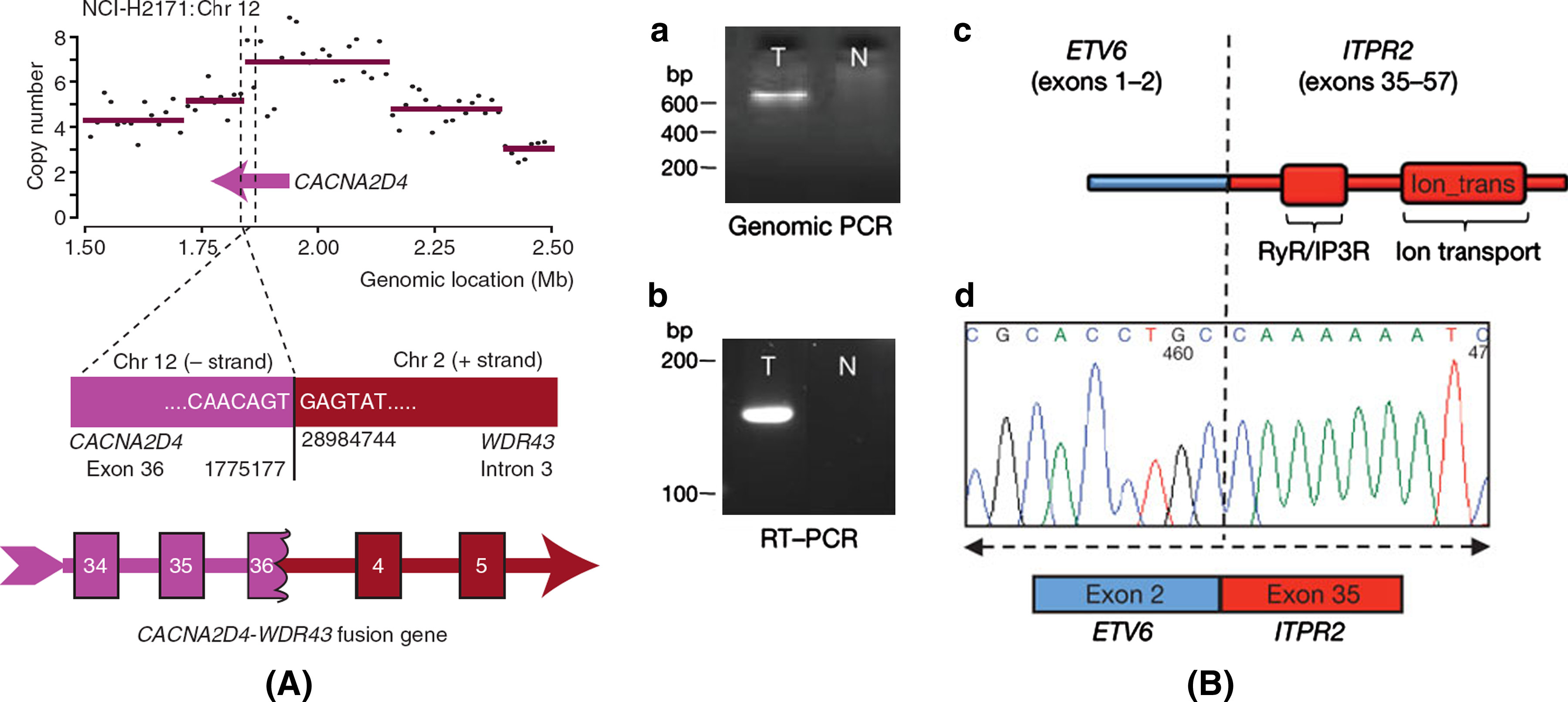
Fusion genes in cancer genomes. (A) CACNA2D4-WDR43 fusion gene identified in the NCI-H2171 lung cancer cell line. The 5′ portion of the CACNA2D4 gene is amplified. A rearrangement breaks the gene in exon 36, fusing it into intron 3 of WDR43. The sequence at the breakpoint creates an almost perfect splice-donor site, resulting in a fusion transcript with a shortened exon 36 from CACNA2D4. (From Campbell et al., 2008.) (B) ETV6-ITPR2 fusion gene in the primary breast cancer PD3668a. [B-a] Across-rearrangement PCR to confirm the rearrangement in genome. [B-b] RT-PCR of RNA between ETV6 exon 2 and ITPR exon 35 to confirm the expressed transcript. N, normal; T, tumor. [B-c] Diagram of the protein domains fused in the ETV6-ITPR2 fusion protein. [B-d] Sequence from RT-PCR product shown in B-b confirming ETV6 exon 2 fused to ITPR2 exon 35. (From Stephens et al., 2009.)

5. Conclusion

Our capability to sequence the entire human genome and other mammalian species has given us an unprecedented opportunity to peer into our origins and decode our own genomes. Based on computational analysis of the genomes of modern mammals, it would be extremely exciting to find out the critical genetic changes that led to the remarkable differences among these species. As the genomic data grows exponentially, the idea of ancestral genome reconstruction is an elegant way to organize a large number of related species, creating a vertical map so that we can navigate the genomes and trace the history from past to present. Even when we study genomic variation in the human population and human disease genomes, it is always important to put the genomic data into the evolutionary context to approach these problems. As Theodosius Dobzhansky said: “Nothing in biology makes sense except in the light of evolution.”

Footnotes

Acknowledgment

We would like to thank Pavel Pevzner, Phillip Compeau, Eugene Koonin, and Ryan Cunningham for helpful suggestions.

Disclosure Statement

No competing financial interests exist.

References

Alekseyev

, Pevzner

2007. Are there rearrangement hotspots in the human genome. PLoS Comput. Biol., 3:e209.

Blanchette

, Green

E.D.

, Miller

, Haussler

2004. Reconstructing large regions of an ancestral mammalian genome in silico. Genome Res., 14:2412–2423.

Bourque

, Pevzner

P.A.

2002. Genome-scale evolution: reconstructing gene orders in the ancestral species. Genome Res., 12:26–36.

Campbell

, Stephens

, Pleasance

et al. 2008. Identification of somatically acquired rearrangements in cancer using genome-wide massively parallel paired-end sequencing. Nat. Genet., 40:722–729.

Dobzhansky

, Sturtevant

1938. Inversions in the chromosomes of Drosophila pseudoobscura. Genetics, 23:28–64.

Fitch

W.M.

1971. Toward defining the course of evolution: minimum change for a specific tree topology. Syst. Zool., 20:406–416.

Green

, Krause

, Ptak

et al. 2006. Analysis of one million base pairs of Neanderthal DNA. Nature, 444:330–336.

Hannenhalli

, Pevzner

P.A.

1995. Transforming cabbage into turnip: polynomial algorithm for sorting signed permutations by reversals. Proc. STOC, 178–189.

Larkin

, Pape

, Donthu

et al. 2009. Breakpoint regions and homologous synteny blocks in chromosomes have different evolutionary histories. Genome Res., 19:770–777.

10.

Lee

, Carvalho

, Lupski

2007. A DNA replication mechanism for generating nonrecurrent rearrangements associated with genomic disorders. Cell, 131:1235–1247.

11.

, Zhang

, Suh

B.B.

et al. 2006. Reconstructing contiguous regions of an ancestral genome. Genome Res., 16:1557–1565.

12.

, Ratan

, Raney

B.J.

et al. 2008. The infinite sites model of genome evolution. Proc. Natl. Acad. Sci. USA, 105:14254–14261.

13.

Margulies

, Cooper

, Asimenos

et al. 2007. Analyses of deep mammalian sequence alignments and constraint predictions for 1% of the human genome. Genome Res., 17:760.

14.

Medvedev

, Stanciu

, Brudno

2009. Computational methods for discovering structural variation with next-generation sequencing. Nat. Methods, 6:13–20.

15.

Miller

, Drautz

, Ratan

et al. 2008. Sequencing the nuclear genome of the extinct woolly mammoth. Nature, 456:387–390.

16.

Miller

, Makova

, Nekrutenko

et al. 2004. Comparative genomics. Annu. Rev. Genomics Hum. Genet., 5:15–56.

17.

Murphy

, Pringle

, Crider

et al. 2007. Using genomic data to unravel the root of the placental mammal phylogeny. Genome Res., 17:413–421.

18.

Nadeau

, Taylor

1984. Lengths of chromosomal segments conserved since divergence of man and mouse. Proc. Natl. Acad. Sci. USA, 81:814–818.

19.

Pevzner

, Tesler

2003. Genome rearrangements in mammalian evolution: lessons from human and mouse genomes. Genome Res., 13:37–45.

20.

Pollard

, Salama

, Lambert

et al. 2006. An RNA gene expressed during cortical development evolved rapidly in humans. Nature, 443:167–172.

21.

Rocchi

, Archidiacono

, Stanyon

2006. Ancestral genomes reconstruction: an integrated, multi-disciplinary approach is needed. Genome Res., 16:1441.

22.

Sankoff

1992. Edit distances for genome comparisons based on non-local operations. Proc. CPM, 121–135.

23.

Sankoff

, Leduc

, Antoine

et al. 1992. Gene order comparisons for phylogenetic inference: evolution of the mitochondrial genome. Proc. Natl. Acad. Sci. USA, 89:6575–6579.

24.

Stephens

P.J.

, McBride

D.J.

, Lin

M.L.

et al. 2009. Complex landscapes of somatic rearrangement in human breast cancer genomes. Nature, 462:1005–1010.

25.

Yancopoulos

, Attie

, Friedberg

2005. Efficient sorting of genomic permutations by translocation, inversion and block interchange. Bioinformatics, 21:3340–3346.

26.

Zhu

, Sanborn

, Diekhans

et al. 2007. Comparative genomics search for losses of long-established genes on the human lineage. PLoS Comput. Biol., 3:e247.