Robustness Analysis of a Boolean Model of Gene Regulatory Network with Memory

Abstract

The response to different kinds of perturbations of a discrete model of gene regulatory network, which is a generalization of the random Boolean network (RBN) model, is discussed. The model includes memory effects, and the analysis pays particular attention to the influence on the system stability of a parameter (i.e., the decay time of the gene products) that determines the duration of the memory effects. It is shown that this parameter deeply affects the overall behavior of the system, with special regard to the dynamical regimes and the sensitivity. Furthermore, a noteworthy divergence in the response of systems characterized by different memory lengths in the presence of either temporary or permanent damages is highlighted, as is the substantial difference, with respect to classical RBNs, between the specific dynamical regime and the landscape of the attractors.

1. Introduction

During previous years, there were several attempts to model the complex set of processes and interactions that represent gene regulation under a systems perspective. While these models differ in features, applications, and results, they have contributed to drawing a coherent picture of the phenomenon (Karlebach and Shamir, 2008).

The seminal work of S. A. Kauffman on random Boolean networks (RBNs) (Kauffman, 1969a,b, 1971) paved the way for further refinements of the original concept, which is that genes can be interpreted as simple elements that can be only “active” or “inactive” (i.e., Boolean) and that their interactions in terms of enhancement or inhibition of the other genes' activation (shaping a network) may give rise to complex dynamics, which are not foreseeable a priori but are responsible for the adaptability, robustness, and evolution of cells in the environment.

Thereafter, knowledge about molecular mechanisms and pathways at the basis of the cells has been increasingly improved, mostly through the outstanding advances in molecular biology and, in particular, in those disciplines usually named with the suffix “-omics” (Lee et al., 2002; Giot et al., 2003; Tyers and Mann, 2003; Han et al., 2004; Li et al., 2004; Alberts et al., 2007; Watson et al., 2008).

Consequently, the integration between the effective reductionist approach and the holistic perspective typical of systems biology (Kitano, 2001, 2002; Noble, 2006; Alon, 2007) is one of the major challenges of the future in the quest for the complete characterization and explanation of gene regulation process. Within this methodological framework, the field defined as complex systems biology (Kaneko, 2006) aims to detect and characterize the general principles of biological systems, in general, and of gene regulation networks, in particular, by means of the concepts and the methods provided by the science of complex systems (Kauffman, 1993).

To this end, in spite of the drastic approximations at its basis, the RBN model has repeatedly proven fruitful in the description of significant quantitative features and important general properties of biological systems (Kauffman, 1993, 1995; Kauffman et al., 2003; Serra et al., 2004, 2007, 2008, 2010; Shmulevich et al., 2005; Ramo et al., 2006).

The principal question raised by this work is whether and how a variation in the “memory” of a system that models the gene regulation process may affect its robustness, with particular attention to the concept of dynamical criticality (Derrida and Pomeau, 1986; Aldana et al., 2003).

Robustness is an essential property of biological systems (Csete and Doyle, 2002) and is manifested through phenomenological properties as the adaptation to environmental changes, the relative insensitivity to the variation of specific parameters, and the resistance of the functions of the system to damage. Plainly, the comprehension of the mechanisms and the principles at its basis turns out to be a fundamental issue in the system-level interpretation of biological systems (Chaves et al., 2006).

On the other hand, it was hypothesized several times that real cells might be operating on or close to the hypersurface in the parameter space that separates the ordered from the disordered regime—sometimes referred as “the edge of chaos” (Langton, 1992)—which would ensure an optimal trade-off between robustness and evolvability (Kauffman, 1995; Shmulevich et al., 2005). The concern is how a variation of the memory affects the belonging of a system to a certain dynamical regime.

The model at the center of the analysis is that of Gene Protein Boolean Network (GPBN) (Graudenzi et al., 2009, 2011). The basic idea is to introduce a form of memory within the classical RBN model, in terms of synthesis and decay times associated to the entities of the system. The model is characterized by the presence of two distinct types of entities: G nodes (the particular portion of genetic information that synthesizes for a specific cellular product, i.e., genes) and P nodes (the products of the gene synthesis, i.e., proteins and RNAs). Both the entities are of the Boolean type, and there is a unique sense in the interaction flow: genes synthesize products, which regulate the activity of genes through fixed interaction pathways. The memory is introduced in the model in the form of a specific lifespan that characterizes the P nodes. Because, as in the case of classical RBNs, the system is deterministic, the time is discrete, and all the entities are updated synchronously, it is possible to study the nature and the features of the limit cycles (that are the only attractors in the case of finite systems1).

It is important to remark that the GPBN model was originally designed to allow a meaningful comparison with the relatively abundant data deriving from time-course microarray experiments, which would be incomparable to the original RBN model, because of the strict assumptions about the synchronization of molecular processes. Moreover, this new model could be an effective instrument to achieve a comprehensive dynamical vision about cellular networks, by means of the integration of time-dependent interaction and activity information (Silvescu and Honavar, 2001; Han et al., 2004; Luscombe et al., 2004).

Note also that some other attempts have been performed in order to introduce timing of molecular processes involved in the regulation within graph-based models of GRN, starting from the work of R. Thomas concerning the logic of the regulatory circuitry (Thomas, 1973, 1991; Thomas and D'Ari, 1990) and that of L. Glass and Kauffman on continuous models of GRN (Glass and Kauffman, 1972, 1973). Since, many refinements have been proposed (Graudenzi et al., 2011).

Preliminary analysis on the landscape and the properties of the attractors, presented in Graudenzi et al. (2009, 2011), proved a clear influence of the introduction of the memory in the system. GPBNs characterized by larger memories show, in fact, a configuration of the landscape of the attractors (usually) typical of more ordered networks, while, on the other hand, the average length of the cycles and that of the transients appear to increase with the increase of the protein lifespan. Furthermore, not all the networks behave in the same way in response to the variation of the memory, confirming the general hypothesis of dynamical heterogeneity of this kind of systems.

In this work, we present an in-depth analysis of different kinds of perturbations, either temporary or permanent, concerning the different entities of the GPBN. The main objective of this work is to understand how the presence and the intensity of the memory affects the robustness of the system under analysis, with particular regard to the characterization of its dynamical regime.

In Section 2, the main features and properties of the GPBN model are briefly described. In Section 3, the robustness analysis of the GPBN model is extensively discussed: we present the results of the analysis of the Derrida plots (Subsection 3.1), of the variation of the Hamming distance in time in presence of temporary perturbations (Subsection 3.2), and of the variation of the average activation values of the nodes (Subsection 3.3), while a theoretical study about the sensitivity in GPBNs is reported in Subsection 3.4 and the analysis of the avalanches consequent to gene knockouts is described in Subsection 3.5. In Section 4, results and further developments of the model are presented.

2. Basic Features of the GPBN Model

For an exhaustive description of the GPBN model, the reader is referred to Graudenzi et al. (2011). There are also reviews and descriptions of the RBN model in the literature (Kauffman, 1993; Aldana et al., 2003; Drossel, 2005, 2008).

A GPBN is an oriented graph in which the (Boolean) entities, G nodes and P nodes, respectively, represent genes and gene products (i.e., proteins or RNAs). In this implementation of the model, there are two possible types of interaction: (a) synthesis links, according to which there is one and only one outgoing link from each G node to each P node; (b) transcriptional regulation links, given by outgoing links from P nodes to G nodes.2 There can be from 0 up to N-1 outgoing links from P to G nodes, as in the classical regulation diagram in RBNs3 (Fig. 1).

FIG. 1.

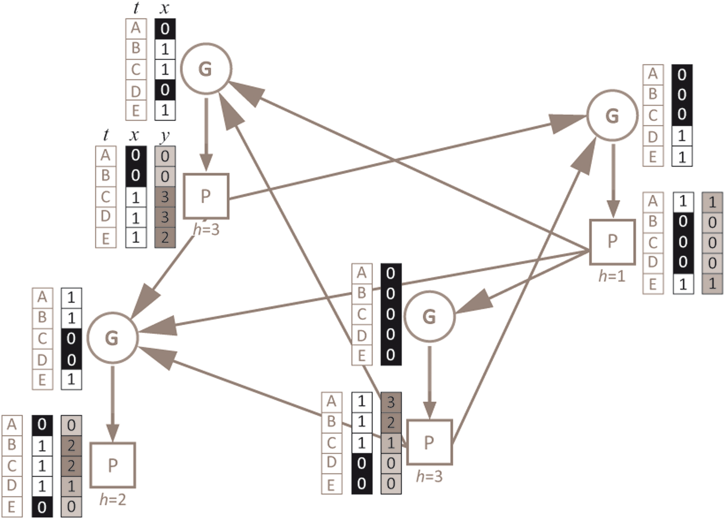
Example scheme of a GPBN. The blue circles correspond to G nodes, while the red squares stand for P nodes; blue links from G to P nodes represent the synthesis links, and red links are the regulative links. Every P node is characterized by a decay time which is indicated below the specific square (y), while every G node is featured by a Boolean function (not shown in the figure). Alongside of G nodes the two columns report respectively the time (t) of this example dynamics (for ease of comprehension indicated by letters, A–E) and the Boolean activation value of that G node (x) at the specific time step. The three columns near the P nodes represent respectively, the time (t), the Boolean activation of that P node (x), and the associated decay phase (h) at time t. This GPBN is composed by 4 G nodes and 4 P nodes (4 G-P node pairs) and characterized by an average connectivity K equal to 2 (being the average connectivity computed on the total of outgoing links from P nodes to G nodes), while a specific time ranging from 1 to 3 (i.e., maximum decay time) is associated randomly to the P nodes. Only 5 time steps of the dynamics are shown.

The main novelty of the model is that synthesis and decay times are associated to every single P node. In this case, we assumed a common unitary synthesis time for all the P nodes (that therefore represents the time unit for the dynamics) and the instantaneity of the regulative interactions of P nodes on G nodes, according to specific Boolean functions associated to G nodes. A uniform distribution of decay times (y_i) is associated to P nodes, ranging from 1 to a structural parameter typical of each realization of GPBN defined as maximum decay time (Y_max from now on). The decay times represent the discrete-length lifespan of the P nodes once activated and provide a form of memory to the system.

It is important to remark that setting Y_max equal to 1 renders the GPBN a classical RBN in terms of structure and dynamics. Hence the GPBN model can be considered as a generalization of the RBN model.

The dynamics of the system is discrete and the updating is synchronous for all the nodes of the network. In detail, if the value of a G node is 1 at time t, the value of its output P node will be 1 at time t + 1. In this case, the value of the P node will remain 1 for a number y_i of time-steps. We define as decay phase, h_i a specific counter that starts from the specific decay time of that protein, y_i and ends in 0; once the P node is activated, the counter is reset to the decay time. Conversely, the value of any G node at time t is determined by a specific Boolean function depending on the Boolean value of its input P nodes at time t.

A k inputs Boolean function f is characterized by 2^k output values. Therefore, there are \documentclass{aastex}\usepackage{amsbsy}\usepackage{amsfonts}\usepackage{amssymb}\usepackage{bm}\usepackage{mathrsfs}\usepackage{pifont}\usepackage{stmaryrd}\usepackage{textcomp}\usepackage{portland,xspace}\usepackage{amsmath,amsxtra}\pagestyle{empty}\DeclareMathSizes{10}{9}{7}{6} \begin{document} $$2^{2^k}$$ \end{document} possible Boolean functions. It is possible to choose the Boolean functions probabilistically according to a specific bias, which is a structural parameter of the system accounting for the probability that the output of a specific Boolean function is 1 on the total number of possible 2^k combination of inputs. Alternatively, it is possible to put constraints on the choice of the set of allowed Boolean functions for a specific network, according to different analysis needs, allowing, for instance, only canalyzing functions, or only biologically plausible functions (Serra et al., 2008).

The topology of the network, the Boolean function associated to each G node, and the decay time associated to the P nodes do not change in time (we deal with the so-called quenched model).

Let \documentclass{aastex}\usepackage{amsbsy}\usepackage{amsfonts}\usepackage{amssymb}\usepackage{bm}\usepackage{mathrsfs}\usepackage{pifont}\usepackage{stmaryrd}\usepackage{textcomp}\usepackage{portland,xspace}\usepackage{amsmath,amsxtra}\pagestyle{empty}\DeclareMathSizes{10}{9}{7}{6} \begin{document} $$ g_i (t) \in \{ 0, 1 \}, p_i (t) \in \{ 0, 1 \}, h_i (t) \in \{ 0, y_i \}, y_i \in \{ 1, Y_{ \max} \}, i = 1, 2, \ldots, N $$ \end{document} denote, respectively, the activation value of the G node i; the activation value, the decay phase, the decay time of the P node I, and the maximum decay time of a GPBN with N G nodes and N P nodes (N G-P node pairs for short from now on). \documentclass{aastex}\usepackage{amsbsy}\usepackage{amsfonts}\usepackage{amssymb}\usepackage{bm}\usepackage{mathrsfs}\usepackage{pifont}\usepackage{stmaryrd}\usepackage{textcomp}\usepackage{portland,xspace}\usepackage{amsmath,amsxtra}\pagestyle{empty}\DeclareMathSizes{10}{9}{7}{6} \begin{document} $$ S (t) = [ g_1 (t), g_2 (t) \ldots g_N (t) ; p_1 (t), p_2 (t) \ldots p_N (t) ; h_1 (t), h_2 (t) \ldots h_N (t ) ] $$ \end{document} represents the activation state of the network at time t. The dynamic of the system is deterministic and the attractors, if N is finite, are cycles of finite length (computed on the three vectors g_i p_i h_i). The average connectivity K is defined as the ratio of the number of outgoing connections of the P nodes over the number of P nodes.

Since many different studies proved a noteworthy dynamical heterogeneity of structurally analogous RBNs and GPBNs (Bastolla and Parisi, 1998; Damiani et al., 2009), the relevance of analyses on single networks is indeed limited, while it is meaningful to perform statistical analyses of a large number of simulations over a large number of networks with the same structural parameters.

3. Robustness Analysis of the GPBN Model

3.1. Derrida plot analysis

One of the most effective instruments to analyze the impact of perturbations on dynamical systems like RBNs and, consequently, to investigate their dynamical behavior is the so-called Derrida plot (Kauffman, 2000). The plot is useful in the discrimination of the dynamical regimes, typically when the combination of structural parameters that would lead to a particular behavior is not known a priori. Given that the GPBN model is a generalization of the RBN, it is sensible to perform this kind of analysis on GPBNs as well: from now on, we will consider as (dynamically) critical those GPBNs characterized by a Derrida curve with a slope in the origin that approximates the value 1.

We performed a certain number of flip perturbations of P nodes on different realizations of GPBNs characterized by the same structural parameters (in terms of topology, average connectivity, bias of the Boolean functions, and Y_max). Derrida plots regarding ensembles of GPBNs distinct for the value of the maximum decay time were finally compared, in order to detect the influence of a variation of this key parameter on the dynamical regime.4

The analyses were made on sets of networks built with parameters typical of the distinct RBNs dynamical regimes, i.e., ordered, chaotic, and critical.5 Notice that all the simulated networks are characterized by a fixed ingoing connectivity (G nodes) equal to K, by a random outgoing connectivity (P nodes), and by a procedure of choice of the Boolean functions through a specific bias p. These are the features typical of the classical RBNs (Fig. 2).

FIG. 2.

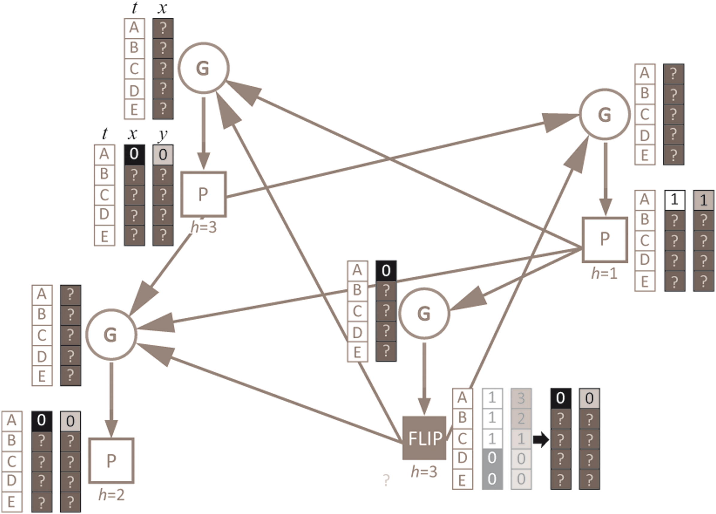
Example scheme of a flip-experiment on the GPBN represented in Figure 1. The P node in the lower right corner is chosen to be flipped in a random initial condition (time = A): its activation value switches from 1 to 0 and, accordingly, its phase skips from 3 to 0. Since all the G nodes (except the corresponding one) have the flipped P node as an input, the flip may influence the first step of the dynamics as well. On the contrary, the state of the other P nodes at time A is not influenced by the flip. For this reason, the state of the G node that is the input of the flipped P node may be influenced by the flip only from the second state of the dynamics on.

3.1.1. Ordered networks

Classical RBNs built with an average connectivity equal to 2 and a bias larger or smaller than 0.5 lay in the ordered dynamical.6 This kind of network presents an average activation value of the nodes that is either larger or smaller than one, according to the specific value of the bias.

The idea at the basis of this analysis is to understand what happens to GPBNs with ordered structural parameters, symmetrical biases, and different memory lengths (given by different values of Y_max). We considered two ensembles of networks: ordered networks with K = 2 and a bias smaller than 0.5 (group A); and ordered networks with K = 2 and a bias larger than 0.5 (group B).

We compared GPBNs belonging to the two distinct groups and characterized with a maximum decay time equal to 1 (that are classical RBNs) with GPBNs with an increasing maximum decay time (i.e., 2, 4, 8, 16). The classical RBNs represent the benchmark from which to start the analysis.

Looking at the values of the Derrida curve close to the origin of the axis (Fig. 3a, Table 1a), we notice that networks characterized by a unitary maximum decay time (i.e., RBNs) present a slope clearly lower than one in both the cases. In particular, the case of a flip of one node only leads to an average Hamming distance around 0.85. The situation becomes different when some memory is introduced within the systems. For GPBNs belonging to group A featured by larger values of the maximum decay time, the slope increases and reaches a value close to 1 (that is the critical value) already when Y_max is equal to 8.

FIG. 3.

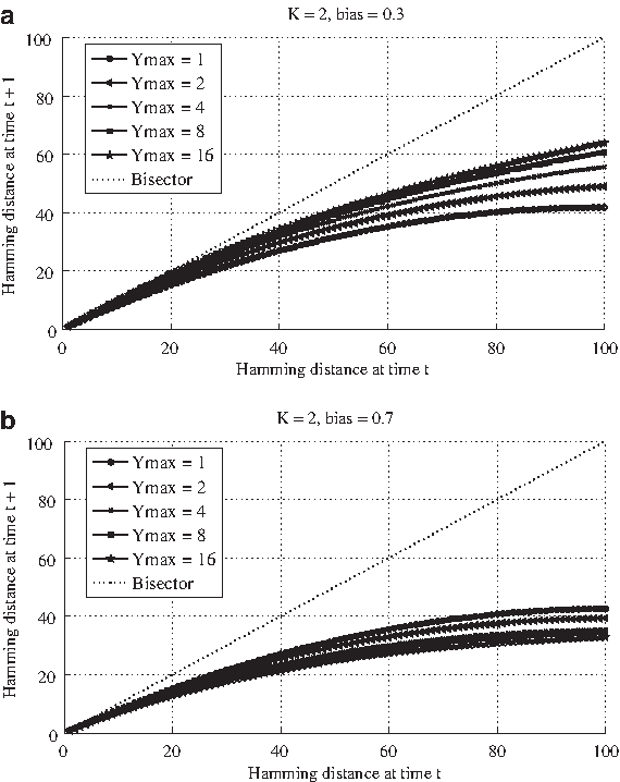
Derrida plot regarding five different ensembles of GPBNs, characterized by a different value of the maximum decay time (i.e., 1, 2, 4, 8, 16). All the networks are composed by N = 100 G-P node pairs, a fixed ingoing connectivity K equal to 2, a random outgoing connectivity and a bias p equal to 0.3, Group A (a); and to 0.7, Group B (b). For every Ymax, 50 different realizations of networks are created; for each realization 100 different simulation runs are performed for every single perturbation experiment, with random initial conditions. Note that GPBNs with Ymax equal to 1 are classical RBNs. On the x-axis is the Hamming distance among the WT and the PT networks at time t (i.e., a random initial condition) on the P nodes. Notice that a Hamming at time t equal to x corresponds to the experiments entailing x flips of P nodes. The value of the curve is computed in this way. Given a certain realization of GPBN, the average value of the Hamming distance at time t + 1 over all the experiments involving x flip is computed. The average value of Hamming distance at time t + 1 is calculated over the different (average) values relative to all the networks belonging to a particular ensembles of GPBNs (characterized by a specific Ymax) is then plotted in correspondence of the coordinate x on the x-axis.

Table 1.

Magnifications of the Plots in Figure 3a,b and Return the First Four Values of the Relative Derrida Plots

(a)
	Hamming distance at time t
	1	2	3	4
Y_max = 1	0.84	1.67	2.49	3.33
Y_max = 2	0.92	1.83	2.75	3.63
Y_max = 4	0.97	1.96	2.95	3.84
Y_max = 8	1.01	2.06	3.05	4.01
Y_max = 16	1.06	2.11	3.12	4.14

(b)
Y_max = 1	0.84	1.65	2.52	3.27
Y_max = 2	0.81	1.61	2.37	3.22
Y_max = 4	0.78	1.57	2.3	3.06
Y_max = 8	0.75	1.53	2.35	2.99
Y_max = 16	0.74	1.46	2.19	2.91

Table 1a refers to the networks belonging to Group A, whereas Table 1b refers to those belonging to Group B.

On the contrary, for networks belonging to group B (Fig. 1b, Table 1b), in correspondence of larger values of the maximum decay times the slopes of the curves diminish, indicating a shift toward the ordered dynamical regime, in apparent contradiction with what just showed about GPBNs characterized by a symmetrical bias. It appears that, in correspondence of biases lower than 0.5, a larger value of Y_max leads to a shift toward the chaotic regime, while for biases larger than 0.5 the shift would be toward the ordered region.

3.1.2. Chaotic networks

RBNs built with an average connectivity larger than 2 and a bias equal to 0.5 are placed in the chaotic dynamical regime (Aldana et al., 2003). The configuration of the activation values throughout the dynamical trajectory is composed, on average, by half of the nodes with value 1 and half of the nodes with value 0.

Looking at the variation of the slopes of the Derrida curves in the case of GPBNs with these structural features and distinct values of Y_max, we can observe how, corresponding to higher values of the Y_max, the slope tends to reduce, indicating a drift toward the ordered region (Fig. 4, Table 2).

FIG. 4.

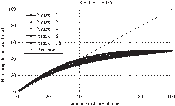
For a precise description of the Derrida plot, please refer to the caption of Figure 3a. We will just indicate the structural features of the GPBNs involved in the experiments. All the GPBNs are composed by N = 100 G-P node pairs, a fixed ingoing connectivity K equal to 3, a random outgoing connectivity and a bias p equal to 0.5. Five different ensembles of GPBNs are analyzed, characterized by a different value of the maximum decay time (i.e., 1, 2, 4, 8, 16). For every MDT, 50 different realizations of networks are created; for each realization 100 different simulation runs are performed within every single perturbation experiment.

Table 2.

Magnification of the Plot in Figure 4, and Returns the First Four Values of the Relative Derrida Plots

	Hamming distance at time t
	1	2	3	4
Y_max = 1	1.5	3.01	4.41	5.86
Y_max = 2	1.42	2.85	4.26	5.54
Y_max = 4	1.39	2.78	4.05	5.31
Y_max = 8	1.32	2.63	3.85	5.18
Y_max = 16	1.32	2.55	3.81	5.03

3.1.3. Critical networks

In the analysis of those networks that, according to the literature on classical RBNs, would lie in the critical regime, one must consider a further distinction. On one side, we have those networks characterized by an average connectivity larger than 2 and biases that according to the phase diagram (Aldana et al., 2003) are typical of dynamically critical behavior; on the other, we have the specific case of GPBNs with K = 2 and a bias p = 0.5, which are the most used parameters in the literature concerning RBNs.

In the former case, the Derrida plots confirm what was observed with critical and chaotic networks, notwithstanding the obvious differences in magnitude. An increase of the maximum decay time forces the GPBNs toward either a more ordered or a more disordered regime in the case of a bias, respectively, larger or smaller than 0.5 (not shown here).

A first hypothesis regarding the results of the analysis of the Derrida plots is then the following: in networks featured by large values of the maximum decay time, the proven symmetry among 0's and 1's in the activation state of the nodes, usually assured by the bias, would be no longer maintained, with the most dramatic effects showing up in correspondence of the highest values of Y_max. A higher maximum decay implies, in fact, that a larger number of P nodes are characterized by a larger decay time (and phase) and, consequently, once activated through the paths of regulation their value will be 1 for a larger number of time steps. This effect would force the system toward a configuration of the nodes with a larger fraction of 1's and, therefore, in dependence on the specific bias, the system would shift respectively toward either a more ordered or more disordered regime: in the case of a bias rather smaller than 0.5 the increase in of Y_max would involve a higher level of disorder, while in case of biases around or larger than 0.5 the pressure would be toward the ordered phase (Fig. 5, Table 3).

FIG. 5.

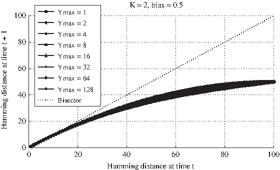
For a precise description of the Derrida plot, refer to the caption of Figure 3a. All the GPBNs are composed by N = 100 G-P node pairs, a fixed ingoing connectivity K equal to 2, a random outgoing connectivity and a bias p equal to 0.5. Five different ensembles of GPBNs are analyzed, characterized by a different value of the maximum decay time (i.e., 1, 2, 4, 8, 16, 32, 64, 128). For every MDT, 50 different realizations of networks are created; for each realization 100 different simulation runs are performed within every single perturbation experiment.

Table 3.

Magnification of the Plot in Figure 5, and Returns the First Four Values of the Relative Derrida Plots

	Hamming distance at time t
	1	2	3	4
Y_max = 1	0.99	1.99	2.95	3.96
Y_max = 2	1.01	1.99	2.96	3.97
Y_max = 4	0.99	1.94	2.96	3.93
Y_max = 8	0.98	2	2.96	3.94
Y_max = 16	0.99	2.01	2.93	3.91
Y_max = 32	1	1.98	2.96	3.93
Y_max = 64	0.99	2.02	2.97	3.93
Y_max = 128	0.98	1.96	2.93	3.91

Nevertheless, observing the Derrida plots regarding GPBNs with K = 2 and bias 0.5, one cannot notice any really significant difference in the shape of the curves, not even in the slope in the origin, in correspondence of different values of Y_max; furthermore, there are no major mismatches among the curves up to very high values of Y_max (e.g., 64 or 128). According to the previous outcomes, one would instead have expected lower values of the curve for a higher Y_max and, consequently, a drift toward the more ordered dynamical regime. Notice also that, as shown in Graudenzi et al. (2011), the analysis of the landscape of the attractors of GPBNs with these structural features and different values of Y_max seems to suggest a shift toward the ordered dynamical regime for larger values of the memory. In the case of critical nets with K = 2, the increase of the maximum decay time appears not to influence the dynamical regime of the considered GPBNs, as indicated by the likeness of the Derrida curves corresponding to networks characterized by even very different values of Y_max.

A possible justification of this counter-intuitive result may be obtained thanks to phase diagram for classical RBNs (Aldana et al., 2003). For different combinations of the bias and the average connectivity, it is possible to determine which dynamical regime the considered network belongs to. Corresponding to the exact combination of K = 2 and p = 0.5, the curve that separates the ordered and the chaotic region is characterized by a plateau: for RBNs characterized by an average connectivity around the value 2 there actually exists a range of different biases, centered in 0.5, that will lead to quite similar dynamical behaviors, at least in response to temporary perturbations. Considering that an increase of Y_max can be roughly interpreted as a shift toward right in the phase diagram, we hypothesize that it actually occurs, while not being detectable with the values of Y_max used in the experiments. Our next analyses aim to confirm this hypothesis.

3.2. Analysis of the Hamming distance by time, in the presence of temporary perturbations

We decided to refine the analysis regarding the robustness of GPBNs with different memories by means of a finer instrument, which is the study of the variation of the Hamming distance by time, in the presence of temporary perturbations. In particular, we focused our attention on one-flip-perturbation experiments on P nodes, successively analyzing the variation of the average Hamming distance, in ensembles of GPBNs characterized by identical structural features and different values of Y_max. The analysis was achieved on the same sets of networks that are analyzed by means of the Derrida plot and that are, respectively, critical, ordered, or chaotic7 (Kauffman, 1993; Aldana et al., 2003; Drossel, 2008).

The analysis made on ordered and chaotic networks substantially supported the results obtained through the Derrida plot analysis, confirming the hypothesis that a larger memory influences the robustness of the networks and their belonging to the dynamical regimes in different ways according to the specific bias. Here we will show the results concerning the ambiguous case of GPBNs with K = 2 and bias = 0.5 only.

In contrast with what observed in Figure 5, different values of Y_max indeed give rise to different curves and to an evident order relation among Y_max and both the slope and the asymptotic values: larger values of Y_max are related to curves that descend more slowly and tend to smaller asymptotic values.

In particular, the case of networks without memory (Y_max = 1, that is the case of classical RBNs) shows a trend that, after a transient, stabilizes around the value 1, and this is what one would expect from critical RBNs. On the contrary, for larger values of Y_max, the dynamics of the systems are characterized by always lower values of the Hamming distance, clearly indicating a better capacity of absorption of the perturbations or, in other words, a higher tendency to the ordered dynamical regime (Fig. 6).

FIG. 6.

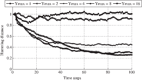
Variation of the average Hamming distance in time (between the WT and the PT cases) in case of one-flip perturbations performed at time t (i.e., a random initial condition) on P nodes (the duration of the perturbation is unitary) on GPBNs. In particular, five sets of GPBNs are analyzed, different for the value of the maximum decay time (i.e., 1, 2, 4, 8, 16). All the GPBNs have these common features: N = 100 G-P node pairs, a fixed ingoing connectivity (G nodes) equal to K = 2, a random outgoing connectivity (P nodes), a bias p = 0.5. For each set of GPBNs, 50 different realizations are created, and for each of them, 100 different perturbation experiments are performed. The final value of the Hamming distance is averaged first on the experiments for each realization and then on the realizations of each ensemble.

In addition to the confirmation of the hypothesis of an actual shift toward the ordered regime also for these networks, this outcome provides a substantiation of the fact that this kind of analysis is more suitable to investigate the dynamical differences of such systems, because it allows to follow the development of the perturbation in time, allowing the system to react: some time is actually needed for the network to absorb or to spread the perturbations, and the Derrida plot does not capture this phenomenon.8

Moreover, this outcome would provide a further evidence to the hypothesis that the presence of a memory in the system drives it to a configuration with more 1's and, according to the cases, either contrasts or favors the tendency towards the ordered regime.

3.3. Analysis of the average activation values

Considered that a possible partial explanation of the observed phenomena may be due to the introduction of a source of asymmetry in the system because of the presence of the decay times, we decided to analyze the time dependence of the average activation value of the nodes.

A statistical analysis on GPBNs built with classical critical parameters (K = 2, p = 0.5 and N = 100) and different values of Y_max (ranging from 1 to 10) was performed.

Looking at the variation of the average activation value of the network on the vector of G nodes only, we can see how, for all the values of Y_max, the average activation value remains around 0.5 (given some possible fluctuations). This result is expected, since the bias and the uniform choice of the Boolean functions assure symmetry of the value of the output, even in the case that the majority of the input P nodes may be equal to 1 (Fig. 7).

FIG. 7.

Variation of the average activation value of the G nodes (given by the ratio of G nodes whose activation value is equal to 1 over the total number N of G-P node pairs) in time (a), of the average activation value of the P nodes (given by the ratio of P nodes whose activation value is equal to 1 over the total number N of G-P node pairs) in time (b), of the average decay phase related to the P in time (c), for different sets of GPBNs characterized by different values of the maximum decay time (ranging from 1 to 10) and the following common features: N = 100 G-P node pairs, a fixed ingoing connectivity (G nodes) equal to K = 2, a random outgoing connectivity (P nodes), a bias p = 0.5. For each set of GPBNs, 50 different realizations are analyzed and the values of the plot is the average computed over the different realizations.

Taking a look, instead, to the average activation value of the P nodes and of their relative phases we can observe a significant phenomenon. Exception made for the case of classical RBN (Y_max = 1), for which the average activation value of the nodes is, as expected, around 0.5, it is evident a correlation among Y_max and the percentage of 1's in P nodes. A peak is detectable after a few time steps and, afterwards, a limit value around 55% is reached for all the values of Y_max larger than 1. A peak is detectable also in the shape of the curves that give account of the average phase of the P nodes of the whole network. After a transient, all the networks reach a different asymptotic value that is roughly given by the equation: \documentclass{aastex}\usepackage{amsbsy}\usepackage{amsfonts}\usepackage{amssymb}\usepackage{bm}\usepackage{mathrsfs}\usepackage{pifont}\usepackage{stmaryrd}\usepackage{textcomp}\usepackage{portland,xspace}\usepackage{amsmath,amsxtra}\pagestyle{empty}\DeclareMathSizes{10}{9}{7}{6} \begin{document} \begin{align*} < h > {\cong } \frac { 1 } { 4 } Y_ { \max } + \frac { 1 } { 4 } \tag { 1 } \end{align*} \end{document}

where <h> is the expected value of the average decay phase associated to the P nodes of a GPBN characterized by a specific maximum decay time, Y_max.

So, the existence of the asymmetry seems to be confirmed in the space of P nodes, and this provides at least a partial explanation of the observed phenomena.

3.4. Sensitivity in GPBNs

In studies about classical RBNs (Serra et al., 2007, 2008), the variable defined as q has been defined as the probability of a randomly chosen node not to change its value at time t if one and only one of its inputs is changed at time t-1. This value depends on the configuration of the Boolean function associated to the nodes and is a key factor in defining the so-called sensitivity: \documentclass{aastex}\usepackage{amsbsy}\usepackage{amsfonts}\usepackage{amssymb}\usepackage{bm}\usepackage{mathrsfs}\usepackage{pifont}\usepackage{stmaryrd}\usepackage{textcomp}\usepackage{portland,xspace}\usepackage{amsmath,amsxtra}\pagestyle{empty}\DeclareMathSizes{10}{9}{7}{6} \begin{document} \begin{align*} \lambda = K (1 - q) \tag{2} \end{align*} \end{document}

which is one of the fundamental parameters in the discrimination of the dynamical regimes and in the detection of the robustness of classical RBNs (Derrida and Pomeau, 1986; Derrida and Stauffer, 1986; Shmulevich et al., 2005; Drossel, 2008). Given this, we decided to analyze the analogous q* for GPBN, also in order to detect how the variation in the memory may affect it.

We developed an analytical formula that takes account of q* for a random GPBN with certain structural features. Note that we will focus our attention on P nodes only (the reason is that the experimental validation can be made through flip experiments, usually made on P nodes). Thus, q* is the probability of a randomly chosen P node not to change its value if one and only one of the input P nodes associated to its corresponding G node changed its value at time t – 1.

Let b_t be the fraction of P nodes whose value is 1 in an arbitrary random condition at time t, and let q be computed on the basis of the choice of the Boolean functions associated to the G nodes (see the Appendix in Serra et al. [2007]): the probability that at time t a randomly chosen G node does not change its value if one of its input P nodes has changed is given by q.

Given that a fraction 1-b_t of the P nodes is characterized by an activation value of 0 at time t and, hence, has 0 remaining lifespan, the probability for these P nodes not to change their value if one of the inputs of their relative G nodes has changed is given by q (case 1).

For the remaining fraction b_t of the nodes we must distinguish two more cases:

For the P nodes that at time t are active and are characterized by a decay phase equal to 1 q* will depend once more from q only (analogously to the case of inactivation) (case 2).

The P nodes whose decay phase is larger than one will surely not change their value (case 3).

Since with Y_max larger than 1 there is a uniform distribution of the decay times on all the P nodes, and given that for an active P node the phase is associated randomly from 1 to the specific decay time we have that for all the different decay times there is a chance of 1/y_i of having a phase equal to 1 (this will depend on q) and y_i-1/y_i to have a phase larger than 1 (this will not be influenced in the change of the input).

The final formula is the following: \documentclass{aastex}\usepackage{amsbsy}\usepackage{amsfonts}\usepackage{amssymb}\usepackage{bm}\usepackage{mathrsfs}\usepackage{pifont}\usepackage{stmaryrd}\usepackage{textcomp}\usepackage{portland,xspace}\usepackage{amsmath,amsxtra}\pagestyle{empty}\DeclareMathSizes{10}{9}{7}{6} \begin{document} \begin{align*} q^ { * } = q \cdot (1 - b_t) + \frac { b_t } { Y_ { \max } } \left(\sum_ { i = 1 } ^ { Y_ { \max } } \frac { q } { y_i } + \frac { y_i - 1 } { y_i } \right) \tag { 3 } \end{align*} \end{document}

We checked the formula through extensive simulations. In particular, one can see in Figure 8 the results of simulations on networks with the classical critical parameters (i.e., a fixed ingoing connectivity K equal to 2, a random outgoing connectivity, a bias p equal to 0.5, 100 G-P node pairs, Y_max ranging from 1 to 50). The match between the analytical formula and the numerical simulation is almost perfect and, as expected, we can notice a clear and direct correlation among the increase of the value of Y_max and that of q*.

FIG. 8.

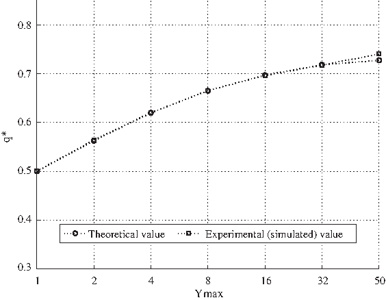
Comparison among the value of the variable q* computed through the analytical formula [3.4.2] and by means of computational simulations. In particular, the simulations regarded groups of 50 realizations of networks with common structural parameters (i.e., N = 100 G-P node pairs, a fixed ingoing connectivity K (G nodes) equal to 2, a random outgoing connectivity (P nodes) and a bias p = 0.5) and different values of Ymax (i.e., 1, 2, 4, 8, 16, 32, 50). The experiment is performed flipping a random P node at time t, observing if the P node corresponding to one of its output G nodes (randomly chosen) changes its value at time t + 1. For each realization, 100 different flips of P nodes have been performed.

This analytical result entails important hints about the concept of “criticality” of such systems: in the case of GPBNs, not only must the bias and average connectivity be considered, but the maximum decay time as well.

3.5. Avalanches in knock-out experiments on GPBNs

In the robustness analysis of GPBNs, we turned our attention towards the knock-out (i.e., permanent silencing) of single G nodes once the network has reached its limit cycle. The root G node of the perturbation is chosen randomly among the nodes whose value is 1 at least once in the activation pattern in the attractor. We then define as the avalanche dimension (avalanche for short) the number of G nodes whose activation pattern in the attractor of the control network is different if compared to the analogous pattern in the attractor of the perturbed one, in a specific knock-out experiment.

Once more, the focus is on the impact of a variation in the maximum decay time on the robustness of the network. Notice that we decide to perform knock-outs on G nodes by analogy to the same experiments executed on classical RBNs and to the experimental methodology of cDNA microarray (Fig. 9).

FIG. 9.

Example scheme of a knock-out experiment on the GPBN represented in Figure 1. The G node in right-upper corner is chose to be knocked-out (supposing that the states A–E in Fig. 1 belong to the attractor) and is permanently clamped to 0 from time = A on (its corresponding P node will be 0 once its phase has run out). The state of the other G nodes will be possibly influenced starting from the second step of the dynamics only, because the first step is determined by the initial condition of the P nodes through the specific Boolean functions. On the other hand, the P nodes may be influenced by the knock-out only from the third step of the dynamics (i.e., C), being the second determined univocally by the state of the G nodes at time = A.

These experiments regarded GPBNs built with different combinations of critical parameters.9 We decided, in fact, to investigate the behavior of critical GPBNs with biases either larger or smaller than 0.5 because of the supposed influence that the introduction of the decay times would entail in relation to the proportion of 0's and 1's usually assured by the bias, and also because of the marked difference in the Derrida curves of these specific networks when characterized by different maximum decay times. The first analyses regarded the variation of average and maximum avalanche, averaged on sets of GPBNs distinct for the value of the maximum decay time.10 Notice that, in this case, the avalanche is defined as the number of G nodes whose activation pattern in the attractor is different in the wild type and in the perturbed cases.

It is surprising to observe (Fig. 10) that the dimensions of the average and maximum avalanche seem to be largely insensitive to the variation of Y_max (ranging from 1 to 10), for all the three different combinations of critical parameters. Indeed, according to the hypotheses illustrated above, a variation of Y_max affects the degree of order in different ways if the bias is smaller, equal to or larger than 0.5, and on the basis of the behavior of classical RBNs one would expect that more ordered RBNs display smaller avalanches. Furthermore, these results are confirmed by experiments with networks of different sizes (ranging from 10 to 1000; not shown here). In Figure 10, we report the case of N = 100 networks. Even more alike are the distributions of the avalanches, which appear not to be affected by the differences in Y_max (Fig. 11).

FIG. 10.

Variation of the mean values of the average avalanche and the maximum avalanche in consequence of knock-out experiments of single G nodes, on GPBNs characterized by the following features: K = 3, p = 0.2111 (a); K = 2, p = 0.5 (b); K = 3, p = 0.7889 (c). All the GPBNs are composed by N = 100 G-P node pairs. For the three combinations of parameters 10 sets of GPBNs have been used in these experiments, distinct for the value of the maximum decay (ranging from 1 to 10). 20 different realizations for each set were built and for each realization 200 knock-out experiments were performed on randomly chosen G nodes (among those G nodes whose activation value is 1 at least once in the limit cycle; the value of the chosen G node is permanently clamped to 0). Notice that the values of average and maximum avalanche are averaged first over the knock-out experiments for each realization and then over the realizations of the different ensembles. The error bars on the plot represent the standard error over the average value.

FIG. 11.

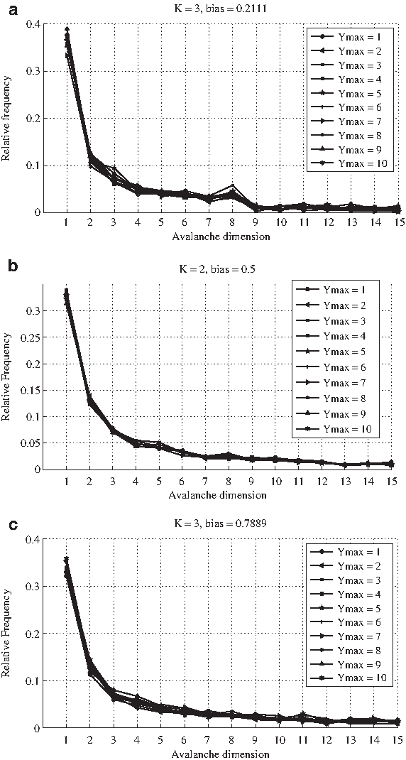
Frequency distribution of the avalanches (up to dimension 15) corresponding to the knock-out experiments on the GPBNs described in the caption of Figure 10, in the three cases, respectively, (a), (b), and (c). On the x-axis is the dimension of the avalanche, and on the y-axis the relative frequency.

Notice that past experiments on RBNs characterized by ordered structural parameters (e.g., K = 2, p = 0.3) showed not only a good robustness in case of temporary perturbations (as we can notice in the Derrida plot of ordered GPBNs with Y_max = 1 in Fig. 3), but also very different values of (average and maximum) avalanches, as well as distinct distributions, in respect to RNBs characterized by more disordered structural parameter (the opposite being for RBNs with disordered structural parameters).

Since we do not detect this difference in GPBNs characterized by maximum decay times that lead to “ordered” (respectively “disordered”) Derrida curves, this may hint at a noteworthy difference between the dynamical properties of GPBNs with a large memory and those of RBNs with ordered structural parameters, at least in the response to permanent perturbations.

A tentative hypothesis could be associated to the nature of the perturbation itself. A certain amount of “memory” could indeed allow to better resist to temporary perturbation, as suggested by the adjustment of the configuration of the space of the attractors and by the usually longer transients corresponding to a larger Y_max. Short perturbations could be absorbed through the effect of longer phases of P nodes. On the contrary, since knock-out perturbations imply a permanent damage to the internal structure of the network, even the long phases after a certain time become ineffective: hence, a longer memory may not be sufficient to improve the robustness of the system. Further analyses are in phase of development to support this hypothesis and provide a meaningful explanation of the phenomenon.

4. Conclusion

The analysis of the robustness of GPBNs characterized by different values of the maximum decay time allowed us to detect a clear influence of this parameter on overall dynamical behavior.

In detail, the variation of Y_max seems to influence the symmetry of the configuration of the activation states of the nodes: an increase of the value of Y_max entails an overall configuration characterized by a larger fraction of 1's. In this way, large values of the maximum decay time would imply a shift toward either the ordered dynamical regime (in case of biases larger or close to 0.5) or the chaotic phase (in case of biases rather smaller than 0.5), at least in regard to the response to temporary perturbations.

Additionally, because, in accord with the phase diagram of classical RBNs, networks specifically built with an average connectivity equal to 2 turn out to be characterized by a similar dynamical regime for a range of different values of the bias (around 0.5), this is reflected on the scarce influence of a variation of Y_max on structurally analogous GPBNs, in terms of response to perturbations. This outcome would suggest that networks designed with these structural parameters, which are the most used in the literature, are indeed particular networks, with distinct properties even when compared with other critical networks.

Furthermore, given what we observed in the analysis of the landscape of the attractors (Graudenzi et al., 2011), we must underline an important difference with the properties of classical RBNs: different responses to perturbations and, accordingly, different dynamical regimes seem not to be necessarily tied with an analogous configuration of the landscape of the attractors, as usually happens with classical RNBs. As shown in Graudenzi et al. (2011), a larger memory entails an adjustment of the landscape of the attractors toward a configuration that is usually typical of more ordered systems, in terms of number of different attractors: on average, GPBNs with larger values of Y_max are characterized by a smaller number of attractors with larger basins of attraction. On the other hand, analyzing the impact of temporary perturbations, we observe that, for instance, GPBNs with a bias lower than 0.5 (and K = 2) in correspondence of increasing values of Y_max present Derrida curves typical of more disordered networks, thus being characterized as more disordered, according to our definition of dynamical criticality.

Another remarkable finding regards the study of knock-out experiments performed on G nodes (in the attractors), which allowed to detect a substantial independence of the size distribution of the avalanches from the maximum decay time. Even GPBNs characterized by long memories do not show an improvement in the robustness to permanent perturbations like knock-outs.

One final remark: the GPBN model has been firstly designed to provide a new effective instrument to interpret heterogeneous large-scale genomic data sets coming from experimental biology, as well to provide tools for reasoning and generate hypothesis about real biological networks. To this extent, studies under way will entail the comparison among the results of the model and those coming from time-course microarray experiments on real organisms, in order to reach important insight about the architecture and the functioning of real networks and to investigate their generic properties like, for instance, the robustness or the dynamical criticality.

Footnotes

Acknowledgments

This work has been partially supported by the Fondazione di Venezia (; DICE project). Interesting discussions with Alessandro Filisetti, Chiara Damiani, Davide De Lucrezia, Andre Ribeiro, and Irene Poli are gratefully acknowledged.

Disclosure Statement

No competing financial interests exist.

¹Other GRN models take into account the fact that the actual level of expression of genes is plainly not Boolean as, for instance, in the case of continuous-variables models (Kaneko, 2006). Nonetheless, we decided to make use of simplified Boolean models for different reasons: first because only in this case it is possible to deal with very large simulated networks, if compared with models that are based, e.g., on ordinary differential equations; and second, to better identify the parameters and the variables responsible for the observed phenomena and to interpret the subsequent results. Obviously, no single model can wholly describe the complex dynamics and phenomenology of biological systems, and this is the reason why the results of different models should be combined to draw an effective picture of the phenomenon.

²Notice that some types of post-translational regulation mechanisms, like those provided, for instance, by mircroRNAs (Griffith-Jones et al., 2006; Zhang and Su, ), can be included in the model simply tuning the Boolean functions of specific nodes. Nevertheless, a straightforward modification of the model could describe also the presence of different classes of interactions as, for instance, the formation of protein complexes or the post-translational regulation.

³Since it has been demonstrated that several mechanisms of auto-regulation are present in real cells (Alon, ), one could relax the constraint of a maximum number of outgoing links equal to N-1. However, we decided to keep the systems as structurally similar as possible to classical RBNs, preserving this structural feature.

⁴The procedure for this kind of experiment is rather straightforward:

The perturbation regards P nodes only, because the dynamics of the system starts from P nodes at time 0.

Given a control network (WT), the perturbation happens at time t, i.e., a random configuration of the activation states of the nodes of the network.

Given a network composed of N G-P node pairs, each perturbation experiment involves the flip of a certain number x (ranging from 1 to N) of randomly chosen P nodes, indistinctly 1→0 or 0→1. Since, in the initial conditions of a GBPN, if a P node is active, a random phase is assigned as initial condition, in this case if the P node is flipped from 0 to 1, a random phase (with uniform probability between 1 and the maximum decay time) will be given. On the contrary, if the node is flipped from 1 to 0, its phase will necessarily become 0.

In this way, it is possible to draw the entire Derrida plot. In the limit case of N flipped P nodes, the initial condition of the PT network will be exactly a mirror configuration of the WT one. Notice that performing an experiment with x flips implies a starting Hamming distance between the WT and the PT network equal to x. This value will be represented in the x-axis of the Derrida plot, which will range from 1 to N.

The perturbation is temporary and it lasts only one time step.

For each value of x a large number of different experiments are performed, involving each time a randomly selected set of x P nodes to flip.

Once that all the experiments regarding a specific value of x are completed, the value of the Derrida curve corresponding to the x coordinate (on the x-axis) is given by the average Hamming distance between the two networks (WT vs. PT) at time t + 1 (averaged on the number of experiments concerning the specific value of x). Notice that the computation of the Hamming distance is performed on the vector of the states of P nodes only.

Once performed all the experiments on a specific set of different realizations of structurally identical GPBNs, characterized by a particular maximum decay time, the final Derrida plot corresponding to that value of Y_max is given by the point-to-point average of the curves of all the different realizations.

⁵It is important to specify that the classification of the dynamical regime holds for classical RBNs, while its generalization to GPBNs is under study. However, the main features of ordered, critical and chaotic regimes are related to the way in which perturbations are handled, so it is surely sensible to observe how perturbations of different sizes are absorbed by networks with different memory lengths.

⁶According to Aldana et al. (), the phase diagram regarding the dynamical regimes of a classical RBN entails only two parameters: the bias p and the average connectivity K. In detail, for each value of p there exist a critical value of the average connectivity K such that the network is in the ordered regime for K < K_kr(p) and in the chaotic regime for K > K_kr(p). The equation is K_kr = [2p(1− p)]⁻¹.

⁷The methodology at the base of the experiments is rather simple.

The perturbation regards P nodes only (see Derrida plot methodology for further details).

Given a control GPBN (WT), the perturbation happens at time t, i.e., a random initial condition.

The perturbation is the flip of one random P node, indistinctly 1→0 or 0→1 (see Derrida plot methodology).

The perturbation is temporary and it lasts one time step.

A certain and possibly large number y of different one-flip perturbations involving each time randomly chosen P nodes are performed.

Once that all the y perturbations are accomplished, the resulting plot gives account of the variation of the average Hamming among the couples of networks (WT vs. PT), from time 0 (at which the Hamming distance is necessarily equal to 1), up to time Z (i.e., the established last time step of the dynamics). Notice that the average is computed over the y experiments for each step of the dynamics.

Eventually, the final value to be plot corresponding to the ensembles of GPBNs featured by different values of the maximum decay time is computed as an average over the (mean) values corresponding to the different realizations of the GPBNs belonging to the ensembles.

⁸Due to the annealed approximation, according to which the quenched structure of the network is not maintained and the possible pathways of reaction of the system simply do not exist.

⁹(a) K = 2, p = 0.5; (b) K = 3, p = 0.2111; (c) K = 3, p = 0.7889 (in addition, all the GPBNs have the following common features: a fixed ingoing connectivity for G nodes equal to K, a random outgoing connectivity for P nodes). Distinct sets of GPBNs have been formed, different for the value of the maximum decay time, ranging from 1 to 10.

¹⁰A certain number of different realizations of structurally identical GPBNs is created, a large number of distinct knock-out experiments on random G nodes are performed on each realization, and the results are finally grouped in ensembles of realizations with different values of Y_max.

References

Alberts

, Bray

, Lewis

et al. 2007. Molecular Biology of the Cell, 5^th. Garland Science: New York.

Aldana

, Coppersmith

, Kadanoff

2003. Boolean dynamics with random couplings, 23–90. Kaplan

, Marsden

, Sreenivasan

K.R.

Perspectives and Problems in Nonlinear Science. Springer Applied Mathematical Sciences Series: Springer, New York.

Alon

2007. An Introduction to Systems Biology. Chapman & Hall/CRC: Boca Raton, FL.

Bastolla

, Parisi

1998. The modular structure of Kauffman networks. Physica D, 115:219–233.

Chaves

, Sontag

E.D.

, Albert

2006. Methods of robustness analysis for Boolean models of gene control networks. Syst. Biol. (Stevenage), 153:154–167.

Csete

M.E.

, Doyle

J.C.

2002. Reverse engineering of biological complexity. Science, 295:1664.

Damiani

, Graudenzi

, Serra

et al. 2009. On the fate of perturbations in critical random Boolean networks. Proc. Eur. Conf. Complex Syst.CD-ROM ISBN:0-9554123-1-5.

Derrida

, Pomeau

1986. Random networks of automata: a simple annealed approximation. Europhys. Lett., 1:45–49.

Derrida

, Stauffer

1986. Phase transitions in two-dimensional Kauffman random network automata. Europhys. Lett., 2:739.

10.

Drossel

2005. Number of attractors in random Boolean networks. Phys. Rev. E, 72:016110.

11.

Drossel

2008. Random Boolean networks, 69–109. Schuster

H.G.

Reviews of Nonlinear Dynamics and Complexity, 1. Wiley-VHC: New York.

12.

Giot

, Bader

J.S.

, Brouwer

et al. 2003. A protein interaction map of Drosophila melanogaster. Science, 302:1727–1736.

13.

Glass

, Kauffman

S.A.

1972. Cooperative components, spatial localization and oscillatory cellular dynamics. J. Theor. Biol., 34:219–237.

14.

Glass

, Kauffman

S.A.

1973. The logical analysis of continuous, non-linear biochemical control networks. J. Theor. Biol., 39:103–129.

15.

Graudenzi

, Serra

, Villani

et al. 2009. Timing of molecular processes in a synchronous Boolean model of genetic regulatory network. Proc. Eur. Conf. Complex Syst.CD-ROM ISBN:0-9554123-1-5.

16.

Graudenzi

, Serra

, Villani

et al. 2011. Dynamical properties of a Boolean model of gene regulatory network with memory. J. Comput. Biol. 10.1089/cmb.2010.0069(in press).

17.

Griffiths-Jones

, Grocock

R.J.

, van Dongen

et al. 2006. miRBase: microRNA sequences, targets and gene nomenclature. Nucleic Acids Res., 34:D140–D144.

18.

Han

J.D.

, Bertin

, Hao

et al. 2004. Evidence for dynamically organized modularity in the yeast protein-protein interaction network. Nature, 430:88–93.

19.

Kaneko

2006. Life: An Introduction to Complex Systems Biology. Springer: Berlin.

20.

Karlebach

, Shamir

2008. Modelling and analysis of gene regulatory networks. Nat. Rev. Mol. Cell Biol., 9:770–780.

21.

Kauffman

S.A.

1969. Homeostasis and differentiation in random genetic control networks. Nature, 224:177.

22.

Kauffman

S.A.

1969. Metabolic stability and epigenesis in randomly constructed genetic nets. J. Theor. Biol, 22:437–467.

23.

Kauffman

S.A.

1971. Gene regulation networks: a theory of their global structure and behavior. Curr. Top. Dev. Biol., 6:145–182.

24.

Kauffman

S.A.

1993. The Origins of Order. Oxford University Press: New York.

25.

Kauffman

S.A.

1995. At Home in the Universe. Oxford University Press: New York.

26.

Kauffman

S.A.

2000. Investigations. Oxford University Press: New York.

27.

Kauffman

S.A.

, Peterson

, Samuelsson

et al. 2003. Random Boolean network models and the yeast transcriptional network. Proc. Natl. Acad. Sci. USA, 100:14796–14799.

28.

Kitano

2001. Foundations of Systems Biology. MIT Press: Cambridge, MA.

29.

Kitano

2002. Computational systems biology. Nature, 420:206–210.

30.

Langton

C.G.

1992. Life at the edge of chaos. Proc. Workshop Synthesis Simulation Living Syst., 41–91.

31.

Lee

T.I.

, Rinaldi

N.J.

, Robert

et al. 2002. Transcriptional regulatory networks in Saccharomyces cerevisiae. Science, 298:799–804.

32.

, Armstrong

C.M.

, Bertin

et al. 2004. A map of the interactome network of the metazoan C. elegans. Science, 303:540–543.

33.

Luscombe

N.M.

, Babu

M.M.

, Yu

H.Y.

et al. 2004. Genomic analysis of regulatory network dynamics reveals large topological changes. Nature, 431:308–312.

34.

Noble

2006. The Music of Life: Biology Beyond the Genome. Oxford University Press: New York.

35.

Ramo

, Kesseli

, Yli-Harja

2006. Perturbation avalanches and criticality in gene regulatory networks. J. Theor. Biol., 242:164–170.

36.

Serra

, Graudenzi

, Villani

2008. Genetic regulatory networks and neural networks. Proc. Ital. Workshop Neural Networks, 109–117.

37.

Serra

, Villani

, Barbieri

et al. 2010. On the dynamics of random Boolean networks subject to noise: attractors, ergodic sets and cell types. J. Theor. Biol., 265:185–193.

38.

Serra

, Villani

, Graudenzi

et al. 2008. The simulation of gene knock-out in scale-free random Boolean models of genetic networks. Networks Heterogeneous Media, 3:333–343.

39.

Serra

, Villani

, Graudenzi

et al. 2007. Why a simple model of genetic regulatory networks describes the distribution of avalanches in gene expression data. J. Theor. Biol., 246:449–460.

40.

Serra

, Villani

, Semeria

2004. Genetic network models and statistical properties of gene expression data in knock-out experiments. J. Theor. Biol., 227:149–157.

41.

Shmulevich

, Kauffman

S.A.

, Aldana

2005. Eukaryotic cells are dynamically ordered or critical but not chaotic. Proc. Natl. Acad. Sci. USA, 102:13439–13444.

42.

Silvescu

, Honavar

2001. Temporal Boolean network models of genetic networks and their inference from gene expression time series. Complex Systems, 11:1–18.

43.

Thomas

1973. Boolean formalization of genetic control circuits. J. Theor. Biol., 42:563–585.

44.

Thomas

1991. Regulatory networks seen as asynchronous automata: a logical description. J. Theor. Biol., 153:1–23.

45.

Thomas

, D'Ari

1990. Biological Feedback. CRC Press: Boca Raton, FL.

46.

Tyers

, Mann

2003. From genomics to proteomics. Nature, 422:193–197.

47.

Watson

J.D.

, Baker

T.A.

, Bell

S.P.

et al. 2008. Molecular Biology of the Gene, 6^th. Benjamin Cummings/Pearson Education: San Francisco.

48.

Zhang

, Su

2009. Small but influential: the role of microRNAs on gene regulatory network and 3'UTR evolution. J. Genet. Genomics, 36:1–6.