Genovo: De Novo Assembly for Metagenomes

Abstract

Next-generation sequencing technologies produce a large number of noisy reads from the DNA in a sample. Metagenomics and population sequencing aim to recover the genomic sequences of the species in the sample, which could be of high diversity. Methods geared towards single sequence reconstruction are not sensitive enough when applied in this setting. We introduce a generative probabilistic model of read generation from environmental samples and present Genovo, a novel de novo sequence assembler that discovers likely sequence reconstructions under the model. A nonparametric prior accounts for the unknown number of genomes in the sample. Inference is performed by applying a series of hill-climbing steps iteratively until convergence. We compare the performance of Genovo to three other short read assembly programs in a series of synthetic experiments and across nine metagenomic datasets created using the 454 platform, the largest of which has 311k reads. Genovo's reconstructions cover more bases and recover more genes than the other methods, even for low-abundance sequences, and yield a higher assembly score. Supplementary Material is available at www.liebertoinline.com/cmb.

1. Introduction

The goal of metagenomic sequencing is to produce a sequence-based summary of the genomic material in a genetically diverse environmental sample. Examples of such environments include biomes of systems such as human gut (Gill et al., 2006; Qin et al., 2010), honey bees (Cox-Foster et al., 2007), or corals (Vega Thurber et al., 2008; Meyer et al., 2009) and also larger ecosystems (Venter et al., 2004; Tyson et al., 2004). These studies advance our systemic understanding of biological processes and communities. In addition, the recovered sequences can enable the discovery of new species (Venter et al., 2004) or reveal details of poorly understood processes (Warnecke et al., 2007). Another set of examples include cancer tumor cells (Warren et al., 2009) and pathogen populations such as HIV viral strains (Wang et al., 2007), where the genetic diversity is associated with disease progression and impacts the effectiveness of the drug treatment regime. Finally, the genetic structure of microbial populations may yield insight into evolutionary mechanisms such as horizontal gene transfer, and enable determination of genetic islands carrying functional toolkits necessary for survival and pathogenicity (Qu et al., 2008).

Such studies are made possible through the use of next-generation sequencing technologies, such as the Illumina Genome Analyzer (GA), Roche/454 FLX system, and AB SOLiD system. Compared to older sequencing methods, these sequencers produce a much larger number of relatively short and noisy reads of the DNA in a sample, at a significantly lower cost.

Automatic tools such as MG-RAST (Meyer et al., 2008) can analyze the reads in a metagenomic sample by comparing them to known genomes, protein families, and functional groups in order to grossly categorize the reads and discover genes. Giving these tools a list of assembled sequences, rather than the shorter and noisier individual reads, helps extract more information from the reads and leads to the discovery of more genes and better functional annotation, as demonstrated by the study of Meyer et al. (2009).

Hence our goal is to accurately reconstruct, given a set of reads, a likely set of DNA sequences that generated these reads. In other words, we are looking for the optimal assembly of the reads. While there are a few de novo assemblers aimed at single sequence reconstruction from short reads (Chaisson and Pevzner, 2008; Zerbino and Birney, 2008; Hernandez et al., 2008; Butler et al., 2008), there are no such tools designed specifically for metagenomics. The specific challenges in this setting stem from uncertainty about the population's size and composition. Additionally, coverage across species is uneven and affected by the species' frequency in the sample. Analysis of the complete populations require methods that can reconstruct sequences even for the low-coverage species. Given the lack of methods designed for a metagenomic environment, researchers resort to methods geared towards single sequence reconstruction.

Such single sequence reconstruction tools commonly frame the problem of sequence assembly as that of finding a path through the read set. A crucial requirement for these algorithms' success is summarized by Chaisson et al. (2009): “[this] approach works best for error-free reads and quickly deteriorates as soon as the reads have even a small number of base-calling errors.” To satisfy this requirement, a large computational effort is devoted to detect and correct read errors before any assembly is even attempted. This becomes even harder in 454, as the average read length is above 100 (and can reach 400b) and the error rate is 0.4% per base (Quinlan et al., 2008), so that a large portion of the reads have an error. This leads to removal of infrequent reads which correspond to poorly sequenced reads or a read from a low frequency species. In the latter case, the assembler's ability to reconstruct a low frequency species is adversely affected.

Our approach to the problem is different. First, we introduce a probabilistic model of a read set. Our model associates a probability to each possible list of sequences that could have given rise to this readset. The formulation of the model takes the form of a generative process that constructs a number of sequences and samples reads from these sequences. Such an assembly of sequences can be seen as a reasonable summary of the read set. We do not a priori assume the number of sequences or their length. The model does, however, favor compact assemblies. Second, we describe an algorithm that reconstructs a likely assembly from a read set. The algorithm accomplishes this by seeking the most probable assembly in an iterative fashion, moving between increasingly likely assemblies via a set of moves designed to increase the probability of the assembly. Intuitively, a move rearranges reads into a more compact assemblies that still accurately represent the whole read set. For example, a prototypical move is one that brings a read that overlaps with a sequence into that sequence. Crucially, the moves are not all greedy, thus allowing some undoing of potential erroneous moves. Convergence is achieved when no reasonable move is available. At this point, we report the assembly with the best probability. This is the assembly that best trades off the compactness and read set representation from among the assemblies that the algorithm explored, thus being a likely candidate for the true set of sequences that generated the reads.

Unlike the other methods, our method does not throw away reads and hence is able to extract more information from the data, which contributes to the discovery of more low-abundance sequences. The joint denoising and assembly of the reads enables us to postpone the decision about which bases are noise and make those decisions based on an assembly rather than in a preprocessing step, thus in principle enabling better assembly, albeit at a higher computational cost. The assembly returned by our algorithm is a full description of the original DNA sequences and how each read maps to them. Hence, Genovo does not only provide a reconstruction of the originating sequences, but also performs read denoising and multiple alignment that scales up to the order of 3 · 10⁵ reads.

The accurate and sensitive reconstruction of populations has been tackled in restricted domains, such as HIV sequencing, both experimentally (Wang et al., 2007) and computationally (Jojic et al., 2008; Eriksson et al., 2008; Zagordi et al., 2009). A probabilistic model, partly similar to ours, was also used in the recent work of Zagordi et al. (2009). However, their approach is applicable only to a very small-scale (10³) set of reads already aligned to a short reference sequence.

We compare the performance of our algorithm to three state of the art short read assembly programs in terms of the number of GenBank bases covered, the number of amino acids recognized by PFAM profiles, and using a score we developed, which quantifies the quality of a de novo assembly using no external information. The comparison is conducted on 9 metagenomic datasets (Qu et al., 2008; Biddle et al., 2008; Breitbart et al., 2009; Cox-Foster et al., 2007; Vega Thurber et al., 2008; Dinsdale et al., 2008) and one single sequence assembly dataset. Genovo's reconstructions show better performance across a variety of datasets. In addition, synthetic tests show that the our method consistently outperforms other methods across a range of sequence abundances and thus is robust to diminishing coverage. Genovo is publicly available online at http://cs.stanford.edu/genovo.

2. Results

2.1. Algorithm overview

Each environmental sample originates from an unknown population of sequences. The number, length, and content of these sequences are uncertain. In order to cope with this uncertainty, we formulate a probabilistic model that represents a potentially unbounded set of DNA sequences, also called contigs, of unknown length. In addition, we model the reads obtained from the environmental sample as noisy copies of contiguous parts of these contigs. Thus, different components of our probabilistic model account for the generation of contigs, the locations from which the reads are copied, and the errors in the copy process. The detailed probabilistic model that captures this precisely is given in the Methods section. This model is the basis for our metagenomic sequencing method, as well as the score we propose for de novo reconstructions.

The dataset of reads obtained from an environmental sample serves as an input to our sequence assembly algorithm. Our model-based approach uses this data to infer the number and the content of the contigs used to “generate” the reads, as well as the reads' location. We call the output of such inference an assembly of the reads (Fig. 1A).

FIG. 1.

(A) An assembly. Thick lines represent contigs, thin lines represent reads. The reads are aligned to match the contigs base-for-base. For clarity, the reads are colored by the contig they map to (green for top contig, purple for bottom). (B) Contig letters are updated from left to right. For each position, count how many letters of each type are aligned to it. These counts induce the distribution from which we sample the letter (red histogram on the right). (C) Updating a location for a single read. A read (dotted line) is removed from the assembly. Likelihood scores are computed for all potential locations of the read (including putting it in a new, empty, contig). These scores induce a discrete distribution (marked by the red histogram). A location is sampled (the red arrow) and the read is aligned to it and added to the assembly. (D) Merge contigs. The ends of two contigs are detected to show high similarity. Likelihood scores are computed for all potential merge locations. The merge with the highest likelihood is performed, provided that it improves the probability of the current assembly. (E) A contig letter might be deleted if many reads are aligned to it with an insertion, thus removing that insertion from their new alignment and introducing a deletion (the red dot) to the alignment of the reads that did not have an insertion in that location. An analogous move for is applied for deletions.

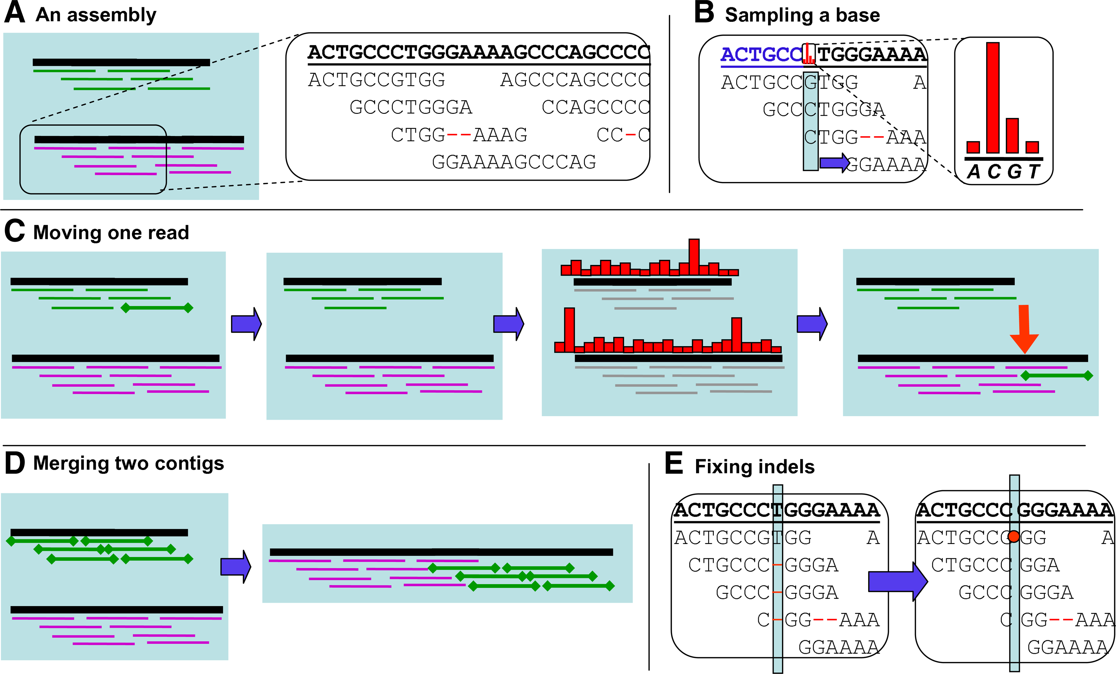
Our algorithm is an instance of the iterated conditional modes (ICM) algorithm (Besag, 1986), which maximizes or samples local conditional probabilities sequentially, in order to reach the assembly with the maximum probability. Starting from an initial random assembly, Genovo performs a random walk on states corresponding to different assemblies. The steps are designed to guide the walk into regions of high probability. The available arsenal of steps includes deterministic hill-climbing steps (that are guaranteed to increase the probability) and stochastic steps (where the next assembly is sampled from a distribution over candidate assemblies, some of them with lower probability), which are necessary in order to avoid getting stuck in a local maximum. We run our algorithm until convergence (200–300 iterations), and then we output the assembly that achieved the highest probability thus far. Running the algorithm multiple times with different random seeds showed no significant influence on the resulting assembly. This suggests that while our algorithm has some stochastic elements, the variability of the output is low.

In Figure 1B–E, we illustrate the four types of steps we use to enable an efficient and correct traversal in the assembly space. One step type, illustrated in Figure 1B, samples a letter for a position in a contig. Another type of step (Fig. 1C), moves a single read either to an already existing contig or to a new one. A single read move involves local alignment, which effectively denoises the read. A third type of step (Fig. 1D) takes even larger steps in the probability space by merging entire contigs. A fourth step type (Fig. 1E) is used to fix indels based on the consensus of the reads.

2.2. Methods compared

While many sequencing technologies are gaining popularity, most of the short-read metagenomic datasets currently available have been sequenced using 454 sequencers (probably due to their longer reads), hence we focus on this technology. Throughout this manuscript, we compare the performance of our algorithm to three other tools: Velvet (Zerbino and Birney, 2008), EULER-SR (Chaisson and Pevzner, 2008), and Newbler, the 454 Life Science de novo assembler. We chose Velvet and Euler due to their high popularity and as representatives of the state of the art. Both these tools were designed for the shorter Illumina reads, but support 454 reads as well and are freely available. Newbler was specifically designed for 454 reads, is extremely popular, and is provided with the 454 machine. As far as we know, this is the only assembler that was designed specifically to meet the assembly needs of the 454 technology. However, the source code for Newbler is unavailable. We also tested SOAPdenovo, as well as ABySS (Simpson et al., 2009), two relatively new assembly programs, but we did not include a detailed comparison with them in the paper because they did not work well on 454 reads.

Running on a set of reads, each method outputs the list of contigs (sequences) that it was able to assemble from the reads. As done in previous studies (Chaisson and Pevzner, 2008; Margulies et al., 2005; Qin et al., 2010), we evaluate only contigs longer than 500bp.

2.3. A single sequence dataset

Before testing the methods on the metagenomic datasets, we benchmarked them on a single sequence assembly task. We used run [SRR:024126] from NCBI short read archive, which contains 110k reads taken from E. coli (length 4.6Mb), sequenced using 454 Titanium. Even though Genovo was not optimized for the single sequence assembly task, it performed on par with the other methods, as Table 1 shows (Newbler achieved a slightly better coverage than Genovo). Genovo and Newbler report much longer contigs than Velvet and Euler (see also Figure 1 in Supplementary Material, available at www.liebertonline.com/cmb).

Table 1.

Comparing the Methods on a Single Sequencing Task

	No. contigs	Total contig length (kb)	N50 (kb)	N90 (kb)	Coverage (%)	Identities (%)
Genovo	129	4693	76.9	25.9	88.4	98.5
Newbler	150	4645	60.4	17.6	88.9	98.5
Velvet	621	4496	10.5	3.6	87.6	98.6
Euler	828	4493	7.6	2.6	86.9	98.6

Contigs were mapped using BLAST to the E. coli reference strand [GenBank:NC_000913.2]. Coverage was computed by taking the union of all matching intervals with length of >400 b. Identities are exact base matches (i.e., not including gaps and mismatches). Nx is the largest value y such that at least x% of the genome is covered by contigs of length of ≥y.

2.4. Metagenomic datasets

We proceeded to compare the methods in a metagenomics setting. The comparison is conducted on eight datasets from six different studies (Table 2), and one synthetic dataset (see Additional File in Supplementary Material). The datasets were chosen so as to reflect common types of population sequencing studies. The first type are studies of viral and bacterial populations inside of another organism; Bee, Fish, Chicken, and Coral were selected as examples of such studies. The second type are studies of environmental samples; The Peru and Microbes dataset are open water samples represent such samples.

Table 2.

Metagenomic Datasets

Name (#reads)	Description (source)
Bee1 (19k), Bee2 (36k)	Samples from two bee colonies. Data obtained by J. DeRisi Lab. (Cox-Foster et al., 2007)
Coral (40k)	Samples from viral fraction from whole Porites compressa tissue extracts [SRR:001078]. (Vega Thurber et al., 2008)
Tilapia1 (50k), Tilapia2 (64k)	Samples from Kent SeeTech Tilapia farm containing microbial [SRR:001069] and viral [SRR:001066] communities isolated from the gut contents of hybrid striped bass. (Dinsdale et al., 2008)
Peru (84k)	Marine sediment metagenome from the Peru Margin subseafloor [SRR:001326]. (Biddle et al., 2008)
Microbes (135k)	Samples from the Rios Mesquites stromatolites in Cuatro Cienagas, Mexico [SRR:001043]. (Breitbart et al., 2009)
Chicken (311k)	Samples of microbiome from chicken cecum. Dataset at http://metagenomics.nmpdr.org, accession 4440283.3 (Qu et al., 2008)
Synthetic (50k)	Metagenomic samples of 13 virus strains, generated using Metasim (Richter et al., 2008), a 454 simulator. See details in Additional file 1.

Accession numbers starting with “SRR” refer to NCBI Short Read Archive (http://www.ncbi.nlm.nih.gov/Traces/sra/sra.cgi). All real datasets were sequenced using 454 GS20, with an average read length of 100–104.

2.4.1. Evaluation metrics

Since for non-simulated data we do not have the actual list of genomes (the “ground truth”) that generated it, exact evaluation of de novo assemblies in metagenomic analysis is hard. We utilize three different indicators for the quality of an assembly. For the first indicator, we BLASTed the contigs produced by each method. Our goal was to estimate both the number of genome bases that the contigs cover, and the quality of that coverage. For each dataset, we used the BLAST hits of all the methods to compile a pool of genomes (downloaded from GenBank) that best represents the consensus among the methods (see Methods). We threw away all the BLAST hits to sequences that did not make it to the pool. We evaluated the quality of the remaining BLAST hits, by computing the BLAST-score-per-base (Bspb) of each hit (the BLAST alignment score divided by the length of the aligned interval). We were then able to show the quantity vs. the quality of the pool bases covered by each method, by asking “How many pool bases were covered by a BLAST hit with a Bspb greater than x?,” and plot it in a graph which we call the BLAST profile. If a method has two BLAST hits that cover the same pool base, we count it only once, and use the higher Bspb value.

The value of the reconstructed sequences lies in the information they carry about the underlying population, such as is provided by the functional annotation of the contigs. Our second indicator evaluated the assemblies based on this information. We decoded the contigs into protein sequences (in all six reading frames) and annotated these sequences with PFAM profile detection tools (Finn et al., 2008). We denote by score_pfam the total number of decoded amino acids matched by PFAM profiles.

The above two indicators can be easily biased when exploring environments with sequences that are not yet in these databases, and hence our third indicator is a score that uses no external information and relies solely on the reads' consistency. Our proposed score, denoted score_denovo, is derived based on the same intuitions as our probabilistic model, which balances the desire to have an assembly with minimal read errors with the desire to have no redundant contigs. For a full description, see Methods.

2.4.2. Performance evaluation

Figure 2 compares the different methods across datasets using score_denovo. Genovo wins on every dataset, with as high as 366% advantage over the second best method. On the synthetic dataset, Genovo assembled all the reads (100.0%) into 13 contigs, one for each virus. The assemblies returned by the other methods are much more fractured—Euler, Velvet, and Newbler returned 33, 47, and 38 contigs, representing only 88%, 36%, and 68% of the reads, respectively. The real datasets with highest score_denovo were Bee1, Bee2, and Tilapia1. Genovo was able to assemble in large contigs 60%, 80%, and 96% of the reads in these datasets, respectively, compared to 30%, 25%, and 59% achieved by the second best method. The low score_denovo values for the other datasets reflect a low or no overlap between most reads in those datasets. Such reads almost always lead to assemblies with many short contigs, regardless of the method used, which drive the score to 0. An example of such dataset is Chicken—all methods produced assemblies which ignored at least 97% of the reads.

FIG. 2.

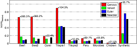
The numbers above the bars represent the improvement (in percentages) between Genovo and the second-best method. To compute score_denovo, we had to complete each list of contigs to a full assembly, by mapping each read to the location that explains it best. Reads that did not align well to any location were treated as singletons—aligned perfectly to their own contig. We could not run EULER-SR on Coral, and the corresponding entry is missing from all figures.

Figure 3 shows the BLAST profile for each method. On the synthetic dataset, Genovo covered almost all the bases (99.7%) of the 13 viruses. Other methods did poorly: Newbler, Euler, and Velvet covered 72.4%, 63.4%, and 39.3% of the bases, respectively. As for the real datasets, in Bee1, Bee2, Tilapia2, and Chicken, many contigs showed a significant match in BLAST (E < 10⁻⁹), and the BLAST profiles provide a good indication for the assembly quality. In those cases, not only does Genovo discover more bases, but it also produces better quality contigs, since Genovo's profile dominates the other methods even on high thresholds for the Bspb value (except on Tilapia2). These differences could also translate to more species. For example, in Bee1, none of Euler's and Newbler's contigs matched in BLAST to Apis mellifera 18S ribosomal RNA gene, even though Genovo and Velvet had contigs that matched it well. On the other datasets most of the contigs did not show a significant match, and hence the genome pools compiled for those datasets are incomplete in the sense that they do not represent all the genomes in the (unknown) ground truth.

FIG. 3.

For each dataset we compiled a pool of GenBank sequences approximating the true sequences. We BLASTed all the contigs of all the methods against the pool. For each method, The curve shows the trade off between the number of the pool bases that its contigs covered (y-axis), and the quality of that coverage (x-axis, measured by BLAST-score-per-base). As we increase the threshold on the quality of the BLAST hits that are included, less bases are covered. The dashed vertical line represents the BLAST-score-per-base of an exact match.The dashed horizontal line represents the total number of bases in the pool covered by at least one method.

Figure 4 compares the methods in terms of the number of amino acids matched by a protein family (PFAM), as measured by score_PFAM. In all datasets, Genovo has the highest score (with the exception of Bee1, where Newbler wins by 260aa), indicating that Genovo's contigs hold more (and longer) annotated regions. For example, in the highly fractured Chicken dataset, our BLAST and PFAM results are markedly higher: 65% more bases were significantly (E < 10⁻⁹) matched in BLAST and 36% more amino acids recognized in PFAM compared to the second best method (Newbler). The difference is also qualitative—the contigs reconstructed by our method were recognized by 84 distinct PFAM families, compared to 67 for Newbler's contigs. It is important to note that in our assembly, the length of matched regions ranged from 54 to 1206aa, with average region length 0f ∼289aa. Similar performance on PFAM matching was achieved on the Tilapia2 dataset, where the number of matched families was 47 (compared to Newbler's 33), and the range of matched regions was 60–1137aa. Such long matched regions could not be recovered from a read-level analysis.

FIG. 4.

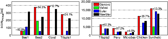
The contigs were translated to proteins in all 6 reading frames. scorePFAM measures how many amino acids were recognized by protein families profilers. Due to the scale difference, results are divided into two figures with the datasets on the right figure having an order of magnitude more annotated amino acids. The numbers above the bars show the change between Genovo and the best of the other methods.

The BLAST and PFAM results should not be taken as the ultimate measure of the reconstruction quality, or the dataset quality, since environmental samples may contain uncultured species that are phylogenetically distant from anything sequenced before. An example of such a dataset is Tilapia1, where almost all the contigs did not match significantly, as shown by the BLAST profiles and score_PFAM, even though they had significant coverage (one of our contigs, with no significant BLAST match, had a segment of 3790 bases with a minimal coverage of ×85 and a mean coverage of ×177). Notably, score_denovo does not suffer from the same problems since it is based on the quality of the read data reconstruction, rather than the presence of a ground truth proxy.

2.5. Robustness tests

We were interested to know how sensitive the model is to sequences that have a low abundance. To check that, we conducted a series of synthetic experiments, each corresponding to increasingly unbalanced population in terms of sequence abundance. In each experiment 50k reads were drawn from 10 sequences, with an exponential drop-off in the abundance of each sequence. Figure 5 shows the average coverage of the two least abundant sequences (i = 9, 10), across the 10 experiments. In the first (leftmost) experiment all sequences had an equal abundance, while at the last one (rightmost) the drop off was 90%. As the abundance gets lower, all methods show reduction covering the sequences (justifiably so, as the fewer reads may no longer cover the entire sequence), but Genovo is able to retain the most coverage of the rare sequences. In the covered regions, the accuracy levels of the reconstruction were the same for all methods, 99.8%. See full details and results in Additional File 1 in Supplementary Material.

FIG. 5.

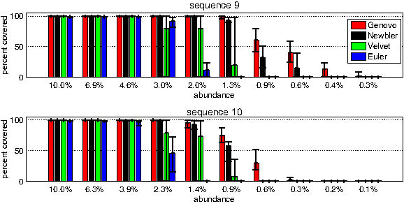
50k simulated reads were extracted from 10 sequences in 10 experiments. Abundance levels were different in each experiment, starting from uniform and getting more and more unbalanced. The graph shows the mean percentage of bases that were covered from the two least abundant sequences across the 10 experiments, as their abundance got worse. Error bars represent the minimum and maximum numbers obtained in 5 replicates. The full set of results across all abundances and allsequences is given in the Supplementary Material.

3. Discussion

Metagenomic analysis involves samples of poorly understood populations. The sequenced sets of reads approximate that population and can yield information about the distribution of gene functions as well as species. However, due to fluctuations of the genomes' coverage, these distributions may be poorly estimated. Furthermore, a read-level analysis may not be able to detect motifs that span multiple reads. Finally, a detailed analysis of events such as horizontal gene transfer will necessitate obtaining both the transposed elements and the genetic context into which they transposed. All of these concerns, in addition to a desire to obtain sequences for novel species, motivate development of sequence assembly methods aimed at problems of population sequencing.

Uncertainty over the sample composition, read coverage, and noise levels make development of methods for metagenomic sequence assembly a challenging problem. We developed a method for sequence assembly that performs well both on biologically relevant scores (based on BLAST and PFAM matches) and on a score that uses no external information. One advantage of our approach is that our probabilistic model is modular, permitting changes to the noise model without the need to modify the rest of the model. Thus, the extensions to other sequencing methodologies, as they are applied to metagenomic data, should be fairly straightforward.

There are two possible causes for variation in the reads: the true biological variation and the sequencing noise. A systematic approach to separating these two sources of variation is predicated on a reasonable model of the measurement noise. We utilize such a noise model based on probabilities of indels and mutations that are in accordance to measured 454 noise profile (Quinlan et al., 2008). This noise model enables us to trade off the two mentioned hypotheses: The measurement noise hypothesis that a set of reads with the same mutation are simply caused by measurement noise vs. the new variant hypothesis that the mutation is genuine and all those reads belong in another sequence (a new variant). These hypotheses have different probabilities that depend on the number of reads and the number of mismatches between the reads and the existing sequences. For example, if the base-mutation rate is 0.1%, and a read length is 100 bases, a relatively simple calculation shows that it takes 20 reads with the same mutation for a new variant hypothesis to be more likely than measurement noise hypothesis.

Extensions of our model can incorporate prior information on the composition of the sequences and would lead to an even more sensitive method that can require a lower coverage to outweigh the measurement noise hypothesis. For example, instead of a uniform prior over the genome letters one can use a prior based on a reference genome. Such a prior will boost the model's sensitivity in detecting variants of that genome, which can be useful when sequencing viral populations or transcriptome. An even more elaborate model will incorporate a model of phylogenetic sequence evolution, allowing us to better distinguish small variations due to local organism evolution. These extensions, although very useful, are outside the scope of this work.

We use a model of 454 noise based on the recent work of Quinlan et al. (2008). We opted not to use quality scores to avoid biases inherent in different base-callers, which vary across software versions of 454 and platforms (GS20 and FLX). Custom base callers and quality scores for 454 and Illumina have been designed by several groups. Assessing the impact of the use of different base callers on the sequence assembly in low coverage scenarios is an interesting problem but out of scope of our paper.

Recently, Illumina reads have been gaining popularity, even for metagenomic studies (Qin et al., 2010). The read quality is increasing and more importantly the reads are getting longer, almost to the level that the original 454 reads were. However, during the writing of this manuscript there were no available Illumina metagenomic datasets, so we had to leverage the available metagenomic datasets for development and assessment of our method, which were and still are predominantly 454 reads. Extending our model to Illumina reads is an important extension of our work, and we believe that the modular structure of our probabilistic model allows replacement of the noise model that was suitable for 454 assembly with the one tuned to Illumina sequencers.

All the methods showed a large range of performance across the different metagenomic datasets. An interesting yet challenging question to ask is what characteristics of a dataset can predict performance. We have found that assemblers universally attained low scores on datasets that had low coverage and a large number of non-overlapping contigs. This suggests that the high diversity in the sample and consequently low coverage significantly impact the maximum achievable score. Some indicators like the diversity of 16 s/18 s sequences may be predictive of the dataset difficulty. Estimation of these frequencies is also challenging as it would require means to compute variant frequencies, estimates from our assemblies being prime candidates. However, a larger number of distinct datasets would be needed for this analysis to be conclusive.

The running time required to construct an assembly can range from 15 minutes on a single CPU for a dataset with 40 k reads up to a few hours for a dataset with 300 k 454 reads, depending not only on the size but also on the complexity of the dataset. Newbler, Velvet and Euler typically provide their results on the order of minutes. Our increase in computational time is on the same scale with the time spent on a next generation sequencing run and it is worthwhile considering the higher quality of the results. Scaling to increasing orders of magnitude is indeed a challenge for next generation assemblers. The largest dataset we tackled was composed of 30 Mbp and did not require parallelization or excessive amounts of memory. While binning algorithms, for example, Wu and Ye (2010), can be used to produce chunks of data and distribute the task of assembly across multiple machines, the datasets we tackled did not require such subdivisions. Further, recently Dirichlet process inference has been shown to be amenable to parallelization (Newman et al., 2009). However this remains a future research direction.

4. Conclusion

The promise of metagenomic studies lies in their potential to elucidate interactions between members of an ecosystem and their influence on the environment they inhabit. In order to begin answering questions about these populations, systematic sequence level analysis is necessary. With advances in sequencing technology and increases in coverage, methods which can explore the space of possible reconstructions will become even more important. The model and method introduced in this paper are well suited to meet these challenges.

5. Methods

5.1. Probabilistic model

To assist the reader, Table 3 summarizes the notation used in the following sections. An assembly consists of a list of contigs, and a mapping of each read to a contiguous area in a contig. The contigs are represented each as a list of DNA letters {b_so}, where b_so is the letter at position o of contig s. For each read x_i, we have its contig number s_i, and its starting location o_i within the contig. We denote by y_i the alignment (orientation, insertions and deletions) required to match x_i base-for-base with the contig. Bold-face letters, such as b or s, represent the set of variables of that type. The subscript −i excludes the variable indexed i from the set.

Table 3.

Notation Table

Variables
x_i	vector of letters of read i (observed)
y_i	alignment (insertions/deletions) of read i
s_i	contig index of read i
o_i	starting offset of read i within contig
b_so	DNA letter in offset o of contig s
ρ_s	controls contig s length
Other parameters
α	controls the number of contigs
p_ins, p_del, p_mis	probability for base insertion, deletion, mismatch
N	number of reads
N_s	number of reads in contig s
\documentclass{aastex}\usepackage{amsbsy}\usepackage{amsfonts}\usepackage{amssymb}\usepackage{bm}\usepackage{mathrsfs}\usepackage{pifont}\usepackage{stmaryrd}\usepackage{textcomp}\usepackage{portland,xspace}\usepackage{amsmath,amsxtra}\pagestyle{empty}\DeclareMathSizes{10}{9}{7}{6} \begin{document}$${ \cal B}$$\end{document}	the DNA letters alphabet (typically {A, C, G, T})

One way to assign a probability to every possible assembly is to describe the full process that generated the reads, from the creation of the originating sequences up to the sequencing noise copying the reads from the sequences. Such model is called a generative model. In this model, the observed variables are the reads x_i, and the hidden variables are the sequences b_so and the location from which each read was copied s_i, o_i plus the alignment y_i. An assembly is hence an assignment to the hidden variables of the model, and once we have a full assignment we can plug it into the model and get a probability.

In our generative process, we first construct a potentially unbounded number of contigs (each has potentially unbounded length), then assign place holders for the beginning of reads in a coordinate system of contigs and offsets, and finally copy each read's letters (with some noise) from the place to which it is mapped in the contig. We deal with the challenge of unbounded quantities by assuming that we have infinitely many of them. Since the number of reads is finite, only a finite number of infinitely many contigs will have any reads assigned to them, and these are the contigs we report. Hence, instead of first deciding how many contigs there are and then assigning the reads to them, we do the opposite—first partition the reads to clusters, and then assign each cluster of reads to a contig. Hence the number of reported contigs will be determined by the number of clusters in the partition generated for the reads.

In order to randomly partition the reads we need a prior over partitions. The Chinese Restaurant Process (CRP) (Aldous, 1983) is such a prior. CRP(α, N) can generate any partition of N items by assigning the items to clusters incrementally. If the first i − 1 items are assigned to clusters \documentclass{aastex}\usepackage{amsbsy}\usepackage{amsfonts}\usepackage{amssymb}\usepackage{bm}\usepackage{mathrsfs}\usepackage{pifont}\usepackage{stmaryrd}\usepackage{textcomp}\usepackage{portland,xspace}\usepackage{amsmath,amsxtra}\pagestyle{empty}\DeclareMathSizes{10}{9}{7}{6} \begin{document} $$s_1 . s_{i - 1}$$\end{document} , then item i joins an existing cluster with a probability proportional to the number of items already assigned to that cluster, or it joins a new cluster with a probability proportional to α. The assignment probability for the last item, given the partition of the previous items is hence given by: \documentclass{aastex}\usepackage{amsbsy}\usepackage{amsfonts}\usepackage{amssymb}\usepackage{bm}\usepackage{mathrsfs}\usepackage{pifont}\usepackage{stmaryrd}\usepackage{textcomp}\usepackage{portland,xspace}\usepackage{amsmath,amsxtra}\pagestyle{empty}\DeclareMathSizes{10}{9}{7}{6} \begin{document} \begin{align*} p ( s_N = s \mid { \bf s } _ { - N } ) = \frac { 1 } { N - 1 + \alpha } \cdot \begin{cases} N_s & \hbox { s is an existing cluster } \\ \alpha & \hbox { s represents a new cluster } \end{cases} \end{align*} \end{document}

where N_s counts the number of items, not including item N, that are in cluster s. One property of the CRP is that the likelihood of a partition under this construction is invariant to the order of the items, and thus this last conditional probability is true for any item i, as we can assume that it is the last one. This conditional probability illustrates another desired property of the CRP, in which items are more likely to join clusters that already have a lot of items. The parameter α controls the expected number of clusters, which in our case represent contigs. In Supplementary Material (Additional File 1), we show how to set it correctly.

The same idea is used to deal with the unbounded length of the contigs. We treat the contigs as infinite in length, stretching from minus infinity to infinity, and then draw the starting points of the reads from a distribution over the integers. The length of the contig is then simply determined by the distance between the two most extreme reads. Since we cannot put a uniform prior over a countably infinite set, and since we want the reads to overlap with each other, we chose to use a symmetric geometric distribution \documentclass{aastex}\usepackage{amsbsy}\usepackage{amsfonts}\usepackage{amssymb}\usepackage{bm}\usepackage{mathrsfs}\usepackage{pifont}\usepackage{stmaryrd}\usepackage{textcomp}\usepackage{portland,xspace}\usepackage{amsmath,amsxtra}\pagestyle{empty}\DeclareMathSizes{10}{9}{7}{6} \begin{document} $${ \cal G}$$\end{document} over the integers that pushes the reads towards the arbitrary “zero.” This center has no meaning except for marking the region of the integer line where reads are more likely to cluster. Formally, this is defined as follows: \documentclass{aastex}\usepackage{amsbsy}\usepackage{amsfonts}\usepackage{amssymb}\usepackage{bm}\usepackage{mathrsfs}\usepackage{pifont}\usepackage{stmaryrd}\usepackage{textcomp}\usepackage{portland,xspace}\usepackage{amsmath,amsxtra}\pagestyle{empty}\DeclareMathSizes{10}{9}{7}{6} \begin{document} \begin{align*} { \cal G} ( o; \rho ) = \left\{ \begin{matrix}0.5 ( 1 - \rho ) ^{ \mid o_t \mid } \rho & o \neq 0 \\ \rho & o = 0\end{matrix} \right. \end{align*} \end{document}

The parameter ρ controls the length of the region from which reads are generated.

The full generative model is described as:

Infinitely many letters in infinitely many contigs are sampled uniformly:

\documentclass{aastex}\usepackage{amsbsy}\usepackage{amsfonts}\usepackage{amssymb}\usepackage{bm}\usepackage{mathrsfs}\usepackage{pifont}\usepackage{stmaryrd}\usepackage{textcomp}\usepackage{portland,xspace}\usepackage{amsmath,amsxtra}\pagestyle{empty}\DeclareMathSizes{10}{9}{7}{6} \begin{document} \begin{align*} b_{so} \sim \hbox{Uniform} ( { \cal B} ) \quad \forall s = 1 \ldots \infty , \forall o = - \infty \ldots \infty \end{align*} \end{document}

where \documentclass{aastex}\usepackage{amsbsy}\usepackage{amsfonts}\usepackage{amssymb}\usepackage{bm}\usepackage{mathrsfs}\usepackage{pifont}\usepackage{stmaryrd}\usepackage{textcomp}\usepackage{portland,xspace}\usepackage{amsmath,amsxtra}\pagestyle{empty}\DeclareMathSizes{10}{9}{7}{6} \begin{document}$${ \cal B}$$\end{document} is the alphabet of the bases (typically \documentclass{aastex}\usepackage{amsbsy}\usepackage{amsfonts}\usepackage{amssymb}\usepackage{bm}\usepackage{mathrsfs}\usepackage{pifont}\usepackage{stmaryrd}\usepackage{textcomp}\usepackage{portland,xspace}\usepackage{amsmath,amsxtra}\pagestyle{empty}\DeclareMathSizes{10}{9}{7}{6} \begin{document}$${ \cal B} = \{ A , C , G , T \} $$\end{document} ).

N empty reads are randomly partitioned between these contigs:

\documentclass{aastex}\usepackage{amsbsy}\usepackage{amsfonts}\usepackage{amssymb}\usepackage{bm}\usepackage{mathrsfs}\usepackage{pifont}\usepackage{stmaryrd}\usepackage{textcomp}\usepackage{portland,xspace}\usepackage{amsmath,amsxtra}\pagestyle{empty}\DeclareMathSizes{10}{9}{7}{6} \begin{document} \begin{align*}{ \bf s} \sim \hbox{CRP} ( \alpha , N )\end{align*}\end{document}

The reads are assigned a starting point o_i within each contig:

\documentclass{aastex}\usepackage{amsbsy}\usepackage{amsfonts}\usepackage{amssymb}\usepackage{bm}\usepackage{mathrsfs}\usepackage{pifont}\usepackage{stmaryrd}\usepackage{textcomp}\usepackage{portland,xspace}\usepackage{amsmath,amsxtra}\pagestyle{empty}\DeclareMathSizes{10}{9}{7}{6} \begin{document} \begin{align*}\begin{matrix} \rho_s \sim \hbox{Beta} ( 1 , \beta ) & \forall s \\ o_i \sim { \cal G} ( \rho_s ) & \forall i = 1..N\end{matrix}\end{align*}\end{document}

The distribution Beta(1, β) is over [0, 1] and has mean 1/(1 + β). We set β = 100.

We assume that the lengths l_i of the reads are already given. The read letters x_i are copied (with some mismatches) from its contig s_i starting from position o_i and according to the alignment y_i (encoding orientation, insertions and deletions):

\documentclass{aastex}\usepackage{amsbsy}\usepackage{amsfonts}\usepackage{amssymb}\usepackage{bm}\usepackage{mathrsfs}\usepackage{pifont}\usepackage{stmaryrd}\usepackage{textcomp}\usepackage{portland,xspace}\usepackage{amsmath,amsxtra}\pagestyle{empty}\DeclareMathSizes{10}{9}{7}{6} \begin{document} \begin{align*}x_i , y_i \sim { \cal A} ( l_i , s_i , o_i , { \bf b} , p_{ins} , p_{del} , p_{mis} ) \qquad \qquad \forall i = 1..N\end{align*} \end{document}

The distribution \documentclass{aastex}\usepackage{amsbsy}\usepackage{amsfonts}\usepackage{amssymb}\usepackage{bm}\usepackage{mathrsfs}\usepackage{pifont}\usepackage{stmaryrd}\usepackage{textcomp}\usepackage{portland,xspace}\usepackage{amsmath,amsxtra}\pagestyle{empty}\DeclareMathSizes{10}{9}{7}{6} \begin{document} $${ \cal A}$$\end{document} represents the noise model known for the sequencing technology (454, Illumina, etc.). In particular, if each read letter has a p_mis probability to be copied incorrectly, and the probabilities for insertions and deletions are p_ins and p_del respectively, then the log-probability log p(x_i, y_i|o_i, s_i, l_i, b) of generating a read in a specific orientation with n_hit matches, n_mis mismatches, n_ins insertions and n_del deletions is \documentclass{aastex}\usepackage{amsbsy}\usepackage{amsfonts}\usepackage{amssymb}\usepackage{bm}\usepackage{mathrsfs}\usepackage{pifont}\usepackage{stmaryrd}\usepackage{textcomp}\usepackage{portland,xspace}\usepackage{amsmath,amsxtra}\pagestyle{empty}\DeclareMathSizes{10}{9}{7}{6} \begin{document} \begin{align*}\log 0.5 + n_ { hit } \log ( 1 - p_ { mis } ) + n_ { mis } \log \left( \frac { p_ { mis } } { \mid { \cal B } \mid - 1 } \right) + n_ { ins } \log ( p_ { ins } ) + n_ { del } \log ( p_ { del } )\end{align*} \end{document}

assuming an equal chance (0.5) to appear in each orientation and an independent noise model. Given an assembly, we denote the above quantity as \documentclass{aastex}\usepackage{amsbsy}\usepackage{amsfonts}\usepackage{amssymb}\usepackage{bm}\usepackage{mathrsfs}\usepackage{pifont}\usepackage{stmaryrd}\usepackage{textcomp}\usepackage{portland,xspace}\usepackage{amsmath,amsxtra}\pagestyle{empty}\DeclareMathSizes{10}{9}{7}{6} \begin{document} $${ \rm score}_{ \rm READ}^i$$\end{document} , where i is the read index.

This model includes an infinite number of b_so variables, which clearly cannot all be represented in the algorithm. The trick is to treat most of these variables as “unobserved,” effectively integrating them out during likelihood computations. The only observed b_so letters are those that are supported by reads, i.e., have at least one read letter aligned to location (s, o). Hence, in the algorithm detailed below, if a contig letter loses its read support, it immediately becomes “unobserved.”

5.2. Algorithm

Our algorithm starts from any initial assembly and takes steps in the space of all assemblies. Recall that each assembly is an assignment to the hidden variables in our model, namely the mapping of every read to the set of contigs (o_i, s_i and y_i for all \documentclass{aastex}\usepackage{amsbsy}\usepackage{amsfonts}\usepackage{amssymb}\usepackage{bm}\usepackage{mathrsfs}\usepackage{pifont}\usepackage{stmaryrd}\usepackage{textcomp}\usepackage{portland,xspace}\usepackage{amsmath,amsxtra}\pagestyle{empty}\DeclareMathSizes{10}{9}{7}{6} \begin{document} $$i = 1.N$$\end{document} ) and the contig letters b_so in the locations that are supported by at least one read. The steps we take are designed to lead us to high probability regions in the space of assemblies. Each step either maximizes or samples a local conditional probability distribution over some hidden variables given the current values for all the other hidden variables. We list below the moves used to explore the space:

5.2.1. Consensus sequence

This type of move (Fig. 1B) updates the sequence letters b_so by maximizing p(b_so|x, y, s, o, b_−so) sequentially for each letter. Let \documentclass{aastex}\usepackage{amsbsy}\usepackage{amsfonts}\usepackage{amssymb}\usepackage{bm}\usepackage{mathrsfs}\usepackage{pifont}\usepackage{stmaryrd}\usepackage{textcomp}\usepackage{portland,xspace}\usepackage{amsmath,amsxtra}\pagestyle{empty}\DeclareMathSizes{10}{9}{7}{6} \begin{document} $$a_{so}^b$$\end{document} be the number of reads in the current assembly that align the letter \documentclass{aastex}\usepackage{amsbsy}\usepackage{amsfonts}\usepackage{amssymb}\usepackage{bm}\usepackage{mathrsfs}\usepackage{pifont}\usepackage{stmaryrd}\usepackage{textcomp}\usepackage{portland,xspace}\usepackage{amsmath,amsxtra}\pagestyle{empty}\DeclareMathSizes{10}{9}{7}{6} \begin{document} $$b \in{ \cal B}$$\end{document} to location (s, o). Since we assumed a uniform prior over the contig letters, it is easy to see that the above conditional probability is maximized by setting \documentclass{aastex}\usepackage{amsbsy}\usepackage{amsfonts}\usepackage{amssymb}\usepackage{bm}\usepackage{mathrsfs}\usepackage{pifont}\usepackage{stmaryrd}\usepackage{textcomp}\usepackage{portland,xspace}\usepackage{amsmath,amsxtra}\pagestyle{empty}\DeclareMathSizes{10}{9}{7}{6} \begin{document} $$b_{so} = \arg \max_{b \in{ \cal B}} a_{so}^b$$\end{document} (ties broken randomly), or in other words, by setting the sequence to be the consensus sequence of the reads in their current mapping.

5.2.2. Read mapping

This move (Fig. 1C) updates the read variables s_i, o_i, y_i, sequentially for each i, by sampling from the probability p(s_i = s, o_i = o, y_i = y|x, y_−i, s_−i, o_−i, b, ρ). First, we remove read i completely from the assembly. The above conditional probability decomposes to: \documentclass{aastex}\usepackage{amsbsy}\usepackage{amsfonts}\usepackage{amssymb}\usepackage{bm}\usepackage{mathrsfs}\usepackage{pifont}\usepackage{stmaryrd}\usepackage{textcomp}\usepackage{portland,xspace}\usepackage{amsmath,amsxtra}\pagestyle{empty}\DeclareMathSizes{10}{9}{7}{6} \begin{document} \begin{align*}p ( s_i = s , o_i = o , y_i = y \mid \cdot ) \propto p ( s_i = s \mid { \bf s}_{ - i} ) p ( o_i = o \mid s_i = s , \rho_{s} ) p ( x_i , y_i = y \mid s_i = s , o_i = o , { \bf b} )\end{align*} \end{document}

In order to make the sampling tractable, we reduce the space by considering for every location (s, o) only the best alignment \documentclass{aastex}\usepackage{amsbsy}\usepackage{amsfonts}\usepackage{amssymb}\usepackage{bm}\usepackage{mathrsfs}\usepackage{pifont}\usepackage{stmaryrd}\usepackage{textcomp}\usepackage{portland,xspace}\usepackage{amsmath,amsxtra}\pagestyle{empty}\DeclareMathSizes{10}{9}{7}{6} \begin{document} $$y^*_{so}$$\end{document} as a possible value for y_i: \documentclass{aastex}\usepackage{amsbsy}\usepackage{amsfonts}\usepackage{amssymb}\usepackage{bm}\usepackage{mathrsfs}\usepackage{pifont}\usepackage{stmaryrd}\usepackage{textcomp}\usepackage{portland,xspace}\usepackage{amsmath,amsxtra}\pagestyle{empty}\DeclareMathSizes{10}{9}{7}{6} \begin{document} \begin{align*}y^*_{so} = \arg \max_y p ( x_i , y_i = y \mid s_i = s , o_i = o , { \bf b} ) .\end{align*}\end{document}

We compute \documentclass{aastex}\usepackage{amsbsy}\usepackage{amsfonts}\usepackage{amssymb}\usepackage{bm}\usepackage{mathrsfs}\usepackage{pifont}\usepackage{stmaryrd}\usepackage{textcomp}\usepackage{portland,xspace}\usepackage{amsmath,amsxtra}\pagestyle{empty}\DeclareMathSizes{10}{9}{7}{6} \begin{document} $$y_{so}^*$$\end{document} using the banded Smith-Waterman algorithm, applied to both read orientations. This includes locations where the read only partially overlaps with the contig, in which case aligning a read letter to an unobserved contig letter entails a probabilistic price of \documentclass{aastex}\usepackage{amsbsy}\usepackage{amsfonts}\usepackage{amssymb}\usepackage{bm}\usepackage{mathrsfs}\usepackage{pifont}\usepackage{stmaryrd}\usepackage{textcomp}\usepackage{portland,xspace}\usepackage{amsmath,amsxtra}\pagestyle{empty}\DeclareMathSizes{10}{9}{7}{6} \begin{document} $$1 / \mid { \cal B} \mid$$\end{document} per letter. Given the vector y*, we can now sample from a simpler distribution over all possible locations (s, o): \documentclass{aastex}\usepackage{amsbsy}\usepackage{amsfonts}\usepackage{amssymb}\usepackage{bm}\usepackage{mathrsfs}\usepackage{pifont}\usepackage{stmaryrd}\usepackage{textcomp}\usepackage{portland,xspace}\usepackage{amsmath,amsxtra}\pagestyle{empty}\DeclareMathSizes{10}{9}{7}{6} \begin{document} \begin{align*}p ( s_i = s , o_i = o \mid { \bf y}^* , \cdot ) & \propto p ( s_i = s \mid { \bf s}_{ - i} ) p ( o_i = o \mid s_i = s , \rho_{s} ) p ( x_i , y^*_{so} \mid s_i = s , o_i = o , { \bf b} ) \\ & \propto N_s \cdot { \cal G} ( o; \rho_s ) \cdot p ( x_i , y^*_{so} \mid s_i = s , o_i = o , { \bf b} ) \end{align*}\end{document}

The weights {N_s}, which count the number of reads in each sequence, encourage the read to join large contigs. As dictated by the CRP, we also include the case where s represents an empty contig, in which case we simply replace N_s with α in the formula above. In that case, the \documentclass{aastex}\usepackage{amsbsy}\usepackage{amsfonts}\usepackage{amssymb}\usepackage{bm}\usepackage{mathrsfs}\usepackage{pifont}\usepackage{stmaryrd}\usepackage{textcomp}\usepackage{portland,xspace}\usepackage{amsmath,amsxtra}\pagestyle{empty}\DeclareMathSizes{10}{9}{7}{6} \begin{document} $$p ( x_i , y_{so}^* \mid \cdot )$$\end{document} term also simplifies to \documentclass{aastex}\usepackage{amsbsy}\usepackage{amsfonts}\usepackage{amssymb}\usepackage{bm}\usepackage{mathrsfs}\usepackage{pifont}\usepackage{stmaryrd}\usepackage{textcomp}\usepackage{portland,xspace}\usepackage{amsmath,amsxtra}\pagestyle{empty}\DeclareMathSizes{10}{9}{7}{6} \begin{document} $$1 / \mid { \cal B} \mid ^{l_i}$$\end{document} , where l_i is the length of the read. We set \documentclass{aastex}\usepackage{amsbsy}\usepackage{amsfonts}\usepackage{amssymb}\usepackage{bm}\usepackage{mathrsfs}\usepackage{pifont}\usepackage{stmaryrd}\usepackage{textcomp}\usepackage{portland,xspace}\usepackage{amsmath,amsxtra}\pagestyle{empty}\DeclareMathSizes{10}{9}{7}{6} \begin{document} $$y_i = y^*_{s_i o_i}$$\end{document} .

As bad alignments render most (s, o) combinations extremely unlikely, we significantly speed up the above computation by filtering out combinations with implausible alignments. A very fast computation can detect locations that have at least one 10-mer in common with the read. This weak requirement is enough to filter out all but a few locations, making the optimization process efficient and scalable. A further speedup is achieved by caching common alignments.

5.2.3. Merge

During the run of the algorithm, as contigs grow and accumulate more reads, it is common to find two contigs that have overlapping ends. Even though the assembly that merges two such contigs into one would have a higher probability, it could take many iterations to reach that assembly if we rely only on the “Read Mapping” step. Reads are likely to move back and forth between the two contigs, especially if they contain a similar number of reads, although eventually chance will make one contig have many more reads than the other, and then the CRP will push the rest of the reads of the smaller contig to the larger one. To speed up this process, we designed a global move (Fig. 1D) where we detect such cases specifically and commit a merge if it increases the likelihood. Specifically, if there are more than 15 k-mers in common between the end of one contig and the beginning of another (we include all possible orientations), we align those ends, re-align the reads in the overlapping interval, and continue with this merged assembly if the overall likelihood had increased.

5.2.4. Fix indels

If the first read that mapped to a previously unsupported area of a contig has an insertion error, then that error is going to propagate into the contig representation. Hence, the “Read Mapping” step will make all the other reads that map to the same location align with an unnecessary insertion. In such locations, this step will propose to delete the corresponding letter in the contig and realign the reads, and accept the proposal if that improves the likelihood (Fig. 1E). We have a similar move for deletions.

5.2.5. Geometric variables

The only hidden variables that are not represented specifically in the assembly are the ρ_s parameters that control the length of the contigs. We set ρ_s to the value that maximizes the probability p(ρ_s| · ) (see Supplementary Material, Additional File 1, for details). Also, any shift by a constant of the starting locations o_i of the reads in a particular contig does not change the assembly. Hence we simply use the shift that maximizes the overall probability. Both the above updates are local optimization moves that do not effect the current assembly.

5.2.6. Chimeric reads

Chimeric reads (Lasken and Stockwell, 2007) are reads with a prefix and a suffix matching distant locations in the genome. In our algorithm, these rare corrupted reads often find their way to the edge of an assembled contig, thus interfering with the assembly process. To deal with this problem we occasionally (every 5 iterations) disassemble the reads sitting in the edge of a contig, thus allowing other correct reads or contigs to merge with it and increase the likelihood beyond that of the original state. If such a disassembled read was not chimeric, it will reassemble correctly in the next iteration, thus keeping the likelihood the same as before.

5.3. Computation of score_denovo

We adopt a view of the metagenomic sequence assembly problem in which two competing constraints are traded off. First, we wish a compact summary of the read dataset. The reconstructed sequences should be reasonably covered and small in number. Second, each read should have a reasonable point of origin in our assembly. score_denovo coherently trades off these constraints.

Given an assembly, denote by S the number of contigs, and by L the total length of all the contigs. We measure the quality of an assembly using the expression \documentclass{aastex}\usepackage{amsbsy}\usepackage{amsfonts}\usepackage{amssymb}\usepackage{bm}\usepackage{mathrsfs}\usepackage{pifont}\usepackage{stmaryrd}\usepackage{textcomp}\usepackage{portland,xspace}\usepackage{amsmath,amsxtra}\pagestyle{empty}\DeclareMathSizes{10}{9}{7}{6} \begin{document} \begin{align*} \sum_i \hbox {score}_{ \rm READ}^i - \log ( \mid { \cal B} \mid ) L + \log ( \mid { \cal B} \mid ) {V_0}S. \end{align*}\end{document}

The first term in the above score penalizes for read errors and the second for contig length, embodying the trade off required for a good assembly. For example, the first term will be optimized by a naive assembly that lays each read in its own contig (so that it is an exact copy of it), but the large number of total bases will incur a severe penalty from the second term. These two terms interact well since they represent probabilities—the first term is the (log) probability for generating each noisy read from the contig bases it aligns to, and the second term is the (log) probability for generating (uniformly) each contig letter. In other words, if you put a read in a region that already has the support of other reads, you pay only for the disagreements between the read and the contig. But if you put that read in an unsupported region, that is, the read is the first one to cover this contig region, then you pay log(0.25) for generating each new letter. If the read does not align well to any supported region in the current assembly, it will be more beneficial to use the read to extend existing contigs or create new contigs than to pay the high “disagreement” cost due to bad alignment.

The third term in the score ensures a minimal overlap of V₀ bases between two consecutive reads. To understand this, assume two reads have an overlap of V bases. If you split the contig into two at this position, the third term gives you a “bonus” of \documentclass{aastex}\usepackage{amsbsy}\usepackage{amsfonts}\usepackage{amssymb}\usepackage{bm}\usepackage{mathrsfs}\usepackage{pifont}\usepackage{stmaryrd}\usepackage{textcomp}\usepackage{portland,xspace}\usepackage{amsmath,amsxtra}\pagestyle{empty}\DeclareMathSizes{10}{9}{7}{6} \begin{document} $$\log ( \mid { \cal B} \mid ) {V_0}$$\end{document} , while the second term penalizes you for \documentclass{aastex}\usepackage{amsbsy}\usepackage{amsfonts}\usepackage{amssymb}\usepackage{bm}\usepackage{mathrsfs}\usepackage{pifont}\usepackage{stmaryrd}\usepackage{textcomp}\usepackage{portland,xspace}\usepackage{amsmath,amsxtra}\pagestyle{empty}\DeclareMathSizes{10}{9}{7}{6} \begin{document} $$\log ( \mid { \cal B} \mid ) V$$\end{document} for adding V new bases to the assembly. Hence, we will prefer to merge the sequences if V > V₀. We set V₀ to 20.

To be able to compare the above score across different datasets, we normalized it by first subtracting from it the score of a naive assembly that puts each read in its own contig, and then dividing this difference by the total length of all the reads in the dataset. We define score_denovo to be this normalized score. See Supplementary Material, Additional File 1, for another derivation of score_denovo, based on our model.

Footnotes

Acknowledgments

We thank J. DeRisi for providing the Bee data. This material is based upon work supported under a Stanford Graduate Fellowship and a National Science Foundation grant (BDI-0345474). An earlier version of this work was presented in RECOMB 2010, Lisbon, Portugal (Laserson et al., ).

Disclosure Statement

No competing financial interests exist.

References

Aldous

1983. Exchangeability and related topics. Ecole Prob. Saint-Flour, XIII:1–198.

Besag

1986. On the statistical analysis of dirty pictures. J. R. Stat. Soc. Ser. B Methodol., 48:259–302.

Biddle

J.F.

, Fitz-Gibbon

, Schuster

S.C.

et al. 2008. Metagenomic signatures of the Peru Margin subseafloor biosphere show a genetically distinct environment. Proc. Natl. Acad. Sci. U.S.A., 105:10583–10588.

Breitbart

, Hoare

, Nitti

et al. 2009. Metagenomic and stable isotopic analyses of modern freshwater microbialites in Cuatro Cinegas, Mexico. Environ. Microbiol., 11:16–34.

Butler

, MacCallum

, Kleber

et al. 2008. ALLPATHS: de novo assembly of whole-genome shotgun microreads. Genome Res., 18:810–820.

Chaisson

M.J.

, Pevzner

P.A.

2008. Short read fragment assembly of bacterial genomes. Genome Res., 18:324–330.

Chaisson

M.J.P.

, Brinza

, Pevzner

P.A.

2009. De novo fragment assembly with short mate-paired reads: does the read length matter? Genome Res., 19:336–346.

Cox-Foster

D.L.

, Conlan

, Holmes

E.C.

et al. 2007. A metagenomic survey of microbes in honey bee colony collapse disorder. Science, 318:283–287.

Dinsdale

E.A.

, Edwards

R.A.

, Hall

et al. 2008. Functional metagenomic profiling of nine biomes. Nature, 452:629–632.

10.

Eriksson

, Pachter

, Mitsuya

et al. 2008. Viral population estimation using pyrosequencing. PLoS Comput. Biol., 4:e1000074.

11.

Finn

R.D.

, Tate

, Mistry

et al. 2008. The Pfam protein families database. Nucleic Acids Res., 36:D281–D288.

12.

Gill

S.R.

, Pop

, Deboy

R.T.

et al. 2006. Metagenomic analysis of the human distal gut microbiome. Science, 312:1355–1359.

13.

Hernandez

, Franois

, Farinelli

et al. 2008. De novo bacterial genome sequencing: millions of very short reads assembled on a desktop computer. Genome Res., 18:802–809.

14.

Jojic

, Hertz

, Jojic

2008. Population sequencing using short reads: HIV as a case study. Pac. Symp. Biocomput., 114–125.

15.

Laserson

, Jojic

, Koller

2011. Genovo: de novo assembly for metagenomes. Proc. RECOMB2010 (this article).

16.

Lasken

R.S.

, Stockwell

T.B.

2007. Mechanism of chimera formation during the multiple displacement amplification reaction. BMC Biotechnol., 7:19.

17.

Margulies

, Egholm

, Altman

W.E.

et al. 2005. Genome sequencing in microfabricated high-density picolitre reactors. Nature, 437:376–380.

18.

Meyer

, Aglyamova

, Wang

et al. 2009. Sequencing and de novo analysis of a coral larval transcriptome using 454 gsflx. BMC Genomics, 10:219.

19.

Meyer

, Paarmann

, D'Souza

et al. 2008. The metagenomics RAST server—a public resource for the automatic phylogenetic and functional analysis of metagenomes. BMC Bioinformatics, 9:386.

20.

Newman

, Asuncion

, Smyth

et al. 2009. Distributed algorithms for topic models. J. Mach. Learn. Res., 10:1801–1828.

21.

Qin

, Li

, Raes

et al. 2010. A human gut microbial gene catalogue established by metagenomic sequencing. Nature, 464:59–65.

22.

, Brulc

J.M.

, Wilson

M.K.

et al. 2008. Comparative metagenomics reveals host specific metavirulomes and horizontal gene transfer elements in the chicken cecum microbiome. PLoS ONE, 3:e2945.

23.

Quinlan

A.R.

, Stewart

D.A.

, Stromberg

M.P.

et al. 2008. Pyrobayes: an improved base caller for SNP discovery in pyrosequences. Nat. Methods, 5:179–181.

24.

Richter

D.C.

, Ott

, Auch

A.F.

et al. 2008. Metasim: A sequencing simulator for genomics and metagenomics. PLoS ONE, 3:e3373.

25.

Simpson

J.T.

, Wong

, Jackman

S.D.

et al. 2009. ABySS: a parallel assembler for short read sequence data. Genome Res., 19:1117–1123.

26.

Tyson

G.W.

, Chapman

, Hugenholtz

et al. 2004. Community structure and metabolism through reconstruction of microbial genomes from the environment. Nature, 428:37–43.

27.

Thurber

R.L.V.

, Barott

K.L.

, Hall

et al. 2008. Metagenomic analysis indicates that stressors induce production of herpes-like viruses in the coral Porites compressa. Proc. Natl. Acad. Sci. USA, 105:18413–18418.

28.

Venter

J.C.

, Remington

, Heidelberg

J.F.

et al. 2004. Environmental genome shotgun sequencing of the Sargasso Sea. Science, 304:66–74.

29.

Wang

, Mitsuya

, Gharizadeh

et al. 2007. Characterization of mutation spectra with ultra-deep pyrosequencing: application to HIV-1 drug resistance. Genome Res., 17:1195–1201.

30.

Warnecke

, Luginbuhl

, Ivanova

et al. 2007. Metagenomic and functional analysis of hindgut microbiota of a wood-feeding higher termite. Nature, 450:560–565.

31.

Warren

R.L.

, Nelson

B.H.

, Holt

R.A.

2009. Profiling model T-cell metagenomes with short reads. Bioinformatics, 25:458–464.

32.

Y.-W.

, Ye

2011. A novel abundance-based algorithm for binning metagenomic sequences using l-tuples. Proc. RECOMB2010 (this issue).

33.

Zagordi

, Geyrhofer

, Roth

et al. 2009. Deep sequencing of a genetically heterogeneous sample: local haplotype reconstruction and read error correction. RECOMB 2009, 345–358.

34.

Zerbino

D.R.

, Birney

2008. Velvet: algorithms for de novo short read assembly using de Bruijn graphs. Genome Res., 18:821–829.

Supplementary Material

Please find the following supplemental material available below.

For Open Access articles published under a Creative Commons License, all supplemental material carries the same license as the article it is associated with.

For non-Open Access articles published, all supplemental material carries a non-exclusive license, and permission requests for re-use of supplemental material or any part of supplemental material shall be sent directly to the copyright owner as specified in the copyright notice associated with the article.

0.00 MB

0.10 MB

Genovo: De Novo Assembly for Metagenomes

Abstract

Abstract

1. Introduction

2. Results

2.1. Algorithm overview

2.2. Methods compared

2.3. A single sequence dataset

2.4. Metagenomic datasets

2.4.1. Evaluation metrics

2.4.2. Performance evaluation

2.5. Robustness tests

3. Discussion

4. Conclusion

5. Methods

5.1. Probabilistic model

5.2. Algorithm

5.2.1. Consensus sequence

5.2.2. Read mapping

5.2.3. Merge

5.2.4. Fix indels

5.2.5. Geometric variables

5.2.6. Chimeric reads

5.3. Computation of score denovo

Footnotes

Acknowledgments

Disclosure Statement

References

Supplementary Material

5.3. Computation of score_denovo