Admixture Aberration Analysis: Application to Mapping in Admixed Population Using Pooled DNA

Abstract

Admixture mapping is a gene mapping approach used for the identification of genomic regions harboring disease susceptibility genes in the case of recently admixed populations such as African Americans. We present a novel method for admixture mapping, called admixture aberration analysis (AAA) that uses a DNA pool of affected admixed individuals. We demonstrate through simulations that AAA is a powerful and economical mapping method under a range of scenarios, capturing complex human diseases such as hypertension and end-stage kidney disease. The method has a low false-positive rate and is robust to deviation from model assumptions. Finally, we apply AAA on 600 prostate cancer-affected African Americans, replicating a known risk locus. Simulation results indicate that the method can yield over 96% reduction in genotyping. Our method is implemented as a Java program called AAAmap and is freely available at http://bioinfo.cs.technion.ac.il/AAAmap.

1. Introduction

Many complex disease studies are currently being conducted using population-based genetic association (The Wellcome Trust Case Control Consortium, 2007). The premise of this method is that affected individuals carry a common variant of a disease-susceptible gene that is in linkage disequilibrium with sampled markers. Hence, the susceptibility locus can be detected via the indirect association between the sampled markers and the disease status. In order to guarantee a sufficiently high power in association studies, thousands of cases and controls are sampled using dense marker panels.

Admixture mapping, also known as mapping by admixture linkage disequilibrium (MALD), offers a more economical alternative to association studies in certain circumstances without sacrificing the statistical power (Smith and O'Brien, 2005). MALD is a gene mapping approach used for the identification of genomic regions harboring disease susceptibility genes in the case of recently admixed populations, i.e., populations that are an admixture of several ancestral populations. African Americans are an example of an admixed population, having both European and African ancestries. The method is applicable when the prevalence of a disease is significantly different between the ancestral populations from which the admixed population was formed. When such a disease is studied, admixed individuals carrying the hereditary disease are expected to show an elevated genomic contribution from the ancestral population that has the higher prevalence of the disease around the disease gene loci. A MALD study is comprised of three main steps. First, a panel of ancestry informative markers (AIM) that differentiate well between ancestral populations is designed. Next, either cases, or both cases and controls are individually genotyped using the AIM panel, and the mosaic of ancestries of each individual is inferred. Finally, the inferred ancestral profiles are scanned in search for an aberration towards the ancestral population with the higher risk, as expected to appear near the disease locus.

The MALD method successfully discovered multiple risk alleles for prostate cancer (Freedman et al., 2006; Haiman et al., 2007), a disease with a higher incident rate in Africans compared to Europeans, and a candidate locus for end-stage kidney disease in African Americans (Kao et al., 2008). Diseases of similar characteristics include stroke, hypertension, and multiple sclerosis; a more comprehensive list of diseases suitable for admixture mapping appears in the method's review by Smith and O'Brien (2005). In all of these cases, the statistical efficiency of MALD stems from the fact that only a few thousand ancestry informative markers are required in order to accurately infer the ancestry of the admixed individuals (Smith et al., 2004). These genetic markers are selected via criteria such as Shannon information content, Fisher information content, or expected mutual information (Rosenberg et al., 2003; Bercovici et al., 2008). Moreover, only a few hundred cases are required for the identification of the ancestral aberration around the disease locus (Reich and Patterson, 2005).

In this article, we present a novel approach for admixture mapping that considerably reduces the genotyping cost of disease studies by applying admixture aberration analysis (AAA) on pooled DNA of affected admixed individuals. Our analysis detects divergence of allele distribution in a pool of samples near a disease locus without the intermediate step of ancestry inference per individual. The inherent aberration in admixture around the disease locus shifts the sampled allele frequencies towards the distribution of the alleles in the ancestry with the higher risk. It is the examination of this shift, evaluated through the estimation of allele frequencies in the pooled sample, that provides the means for our pooled mapping method (Fig. 1).

FIG. 1.

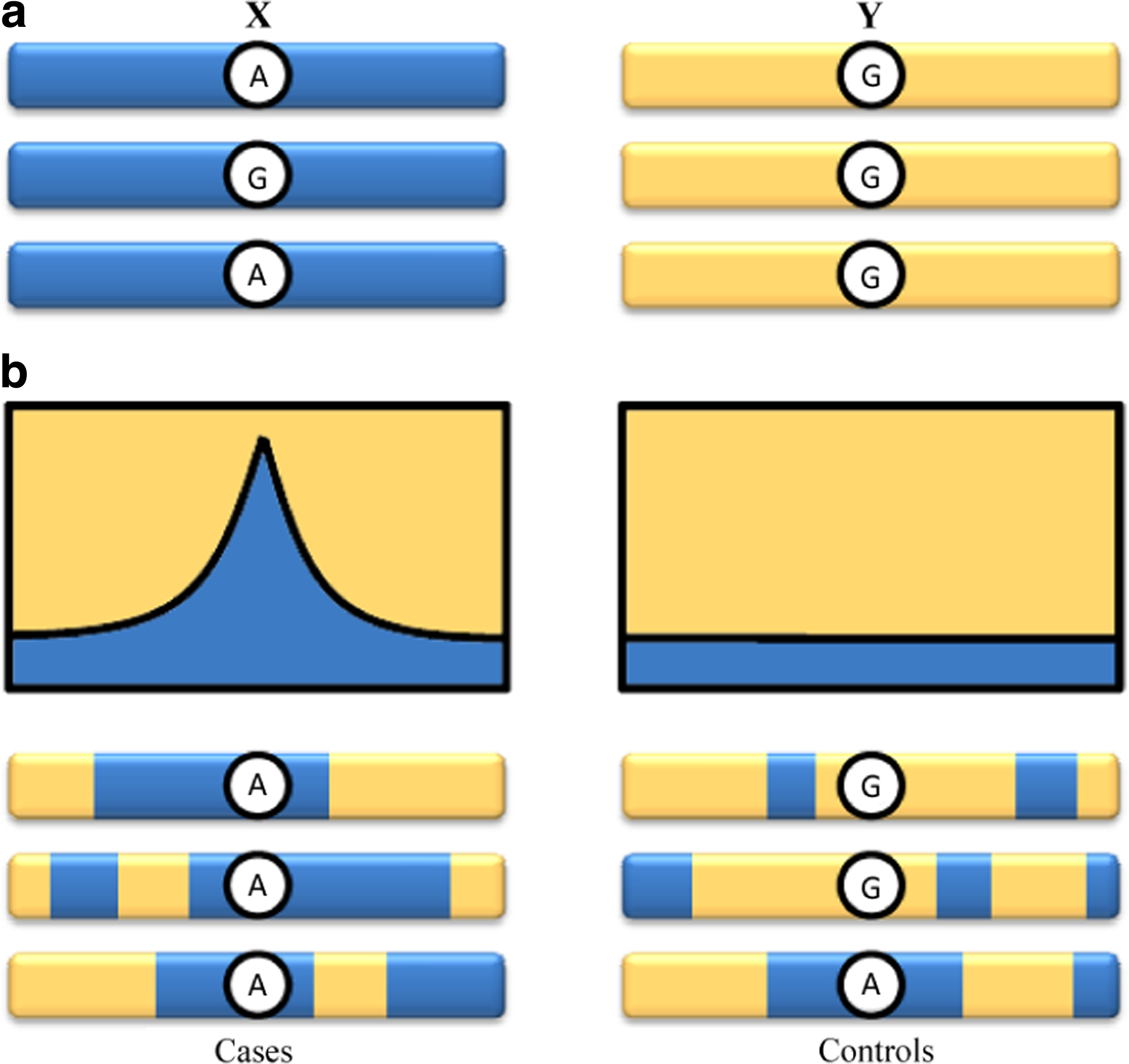
An illustration of admixture aberration. (a) Two distinct ancestral populations, X and Y, expressing a different distribution of alleles at a particular location. The greater the distance between allele distributions, the more informative the marker is regarding ancestry. (b) A sample of admixed individuals, descendants of the ancestral populations X and Y. In case of a disease with higher prevalence in population X, the affected sample will exhibit a higher contribution from population X near the disease locus, as indicated by the graph on the left. Hence, in the affected individuals, the distributions of alleles near the disease locus bears a higher resemblance to that of population X. The healthy admixed individuals show a contribution of populations X and Y that corresponds to the admixture process.

Current MALD studies mainly differ in the informative panel of choice and the method used for ancestry inference. Patterson et al. (2004) presented a method that employs a hidden Markov model (HMM) for the estimation of ancestry along the genome. The HMM was integrated into a Markov chain Monte Carlo (MCMC) method to account for the uncertainties in model parameters. Tang et al. (2006) extended previous methods by modeling linkage-disequilibrium in the ancestral populations using a Markov Hidden Markov model (MHMM), namely, dependency between adjacent markers evident in the ancestral populations was modeled. An inference framework developed in Bercovici and Geiger (2009) enables the incorporation of more complex probability models that account for linkage disequilibrium in the ancestral populations. An earlier work by Chakraborty and Weiss (1988) suggested mapping by directly assessing divergence from admixture linkage-disequilibrium, as expected near disease loci.

DNA pooling has been suggested as a practical way to reduce the cost of large-scale association studies (Sham et al., 2002). Rather than analyzing thousands of cases and controls that were sampled separately, association analysis was first applied on pooled cases and pooled controls in the work of Arnheim et al. (1985). Steer et al. (2006) have recently demonstrated the feasibility of pooled association studies using high-resolution microarrays for rheumatoid arthritis. Zeng and Lin (2005) examined the analysis of pooled DNA, extending the single-marker association methods to haplotype association using a likelihood-based approach. Kirov et al. (2006) investigated the accuracy by which the allele frequency difference between pools can be estimated. This work was extended by Wilkening et al. (2007) for higher resolution SNP microarrays of 250K. Pooling was also used in QTL studies. For example, Darvasi and Soller (1994) presented a statistical test of marker-QTL linkage based on selective pools of individuals with extreme quantitative trait values.

The main contribution of this article is the introduction of pooling to admixture mapping, and the demonstration of its power to the mapping of disease susceptibility loci. Pooling is a far more effective tool for admixture mapping in comparison to association studies. In the case of a recently formed admixed population, the linkage-disequilibrium patterns generated by the admixture process stretch over regions of several centimorgans, resulting in a wider effect which is easier to detect. In addition, using ancestry informative markers improves the ability to locate deviations of LD and marker distribution from those expected by the admixture process alone. The efficiency of our pooled AAA method has been established through simulation and via analysis of diseases that are currently being studied using the non pooled MALD approach. Specifically, we first develop the aberration analysis method based on a window of markers while accounting for linkage disequilibrium in the ancestral populations. We then determine the method's power through simulations. We show, for example, that a power of over 70% is achieved in a simulated study of an African American population carrying a disease with ethnicity relative risk of 1.3, comparable with end-stage kidney disease, using seven pools of 200 individuals with four repetitions. The results in this case indicate a more than 25-fold decrease in genotyping versus a non-pooled MALD method. We also demonstrate the strength of our pooled method on a sample of African American cases of prostate cancer, replacing 600 independently measured individuals with a single simulated pool. The result demonstrate that a significant signal (LOD 7.2) is obtained near the risk locus found by Amundadottir et al. (2006) and Freedman et al. (2006). Finally, we discuss the robustness of our method to measurement errors and to deviation from model assumptions.

Our method is implemented as a Java program called AAAmap and is freely available at http://bioinfo.cs.technion.ac.il/AAAmap.

2. Methods

2.1. Definitions and model assumptions

The genome of a recently admixed individual is a mosaic of long, single ancestry, chromosomal segments. We use the following definitions to describe these segments in admixed individuals. An admixed chromosome is a chromosome that originated from more than one ancestral population. A post admixture recombination (PAR) point is a recombination point in which either two chromosomes from different populations crossed, or two chromosomes crossed where at least one of the chromosomes is an admixed chromosome. A (PAR) block is a chromosomal segment limited by two consecutive PAR points, or by a chromosome edge and its closest PAR point. An immediate implication of these definitions is that every PAR block originated from a single ancestral population, designated as the ancestry of the block, for otherwise the block would have been further divided. In our model, we assume that the ancestry of PAR blocks are mutually independent. We further assume that given the ancestry of a PAR block, the markers within that PAR block are independent of the markers outside the PAR block and are determined strictly according to the distribution that corresponds to the ancestry of that PAR block (Bercovici et al., 2008). The markers within a PAR block are assumed to be dependent, accounting for the background linkage-disequilibrium in the ancestral populations.

Consider an admixed population that originated from two ancestral populations X and Y. Each ancestral population may have a different prevalence for a disease. A common way to characterize the disease risk attributed to the ancestral profile is by the ethnicity relative risk (ERR) which measures the increased risk due to an additional allele from population Y. Under a multiplicative disease model, ERR is defined as \documentclass{aastex}\usepackage{amsbsy}\usepackage{amsfonts}\usepackage{amssymb}\usepackage{bm}\usepackage{mathrsfs}\usepackage{pifont}\usepackage{stmaryrd}\usepackage{textcomp}\usepackage{portland,xspace}\usepackage{amsmath,amsxtra}\pagestyle{empty}\DeclareMathSizes{10}{9}{7}{6} \begin{document} \begin{align*} r = \frac { \psi ( XY ) } { \psi ( XX ) } = \frac { \psi ( YY ) } { \psi ( XY ) } \tag { 1 } \end{align*} \end{document}

where ψ(·) is the probability of the disease given that the ancestry pair at the disease susceptibility locus is either XX, XY, or YY.

When studying an admixed population with an hereditary disease characterized by an ERR ≠ 1, the regions around the disease loci are expected to show an aberration towards the ancestry with the higher risk, shifting the distribution of nearby allele frequencies. Our method scans through the genome, computing for each examined location the ratio between the likelihood of the measured allele frequencies under the assumption of a close disease locus and the likelihood of the measured frequencies under the null assumption of no disease: \documentclass{aastex}\usepackage{amsbsy}\usepackage{amsfonts}\usepackage{amssymb}\usepackage{bm}\usepackage{mathrsfs}\usepackage{pifont}\usepackage{stmaryrd}\usepackage{textcomp}\usepackage{portland,xspace}\usepackage{amsmath,amsxtra}\pagestyle{empty}\DeclareMathSizes{10}{9}{7}{6} \begin{document} \begin{align*} \Lambda_0 = \frac { P ( S \mid \hbox { nearby disease locus } ) } { P ( S \mid \hbox { no disease } ) } \tag { 2 } \end{align*} \end{document}

where S are the observed allele frequencies. Since the computation of this likelihood becomes intractable as the number of samples and markers grow, we approximate these probabilities via the multivariate central limit theorem over a window of markers. This approximate measure, denoted Λ, is used in the reported results. In the remaining method section, we derive the distribution of alleles under the two hypothesis, and the Λ score. We first assume a window with a single marker and then extend the results to multi-marker windows.

2.2. Single marker analysis

We first compute the probability P(J|d) of a bi-allelic marker \documentclass{aastex}\usepackage{amsbsy}\usepackage{amsfonts}\usepackage{amssymb}\usepackage{bm}\usepackage{mathrsfs}\usepackage{pifont}\usepackage{stmaryrd}\usepackage{textcomp}\usepackage{portland,xspace}\usepackage{amsmath,amsxtra}\pagestyle{empty}\DeclareMathSizes{10}{9}{7}{6} \begin{document} $$J \in \{ 0 , 1 \}$$ \end{document} of an individual, given the individual is affected (denoted by d). This probability is given by \documentclass{aastex}\usepackage{amsbsy}\usepackage{amsfonts}\usepackage{amssymb}\usepackage{bm}\usepackage{mathrsfs}\usepackage{pifont}\usepackage{stmaryrd}\usepackage{textcomp}\usepackage{portland,xspace}\usepackage{amsmath,amsxtra}\pagestyle{empty}\DeclareMathSizes{10}{9}{7}{6} \begin{document} \begin{align*} P ( J \mid d ) = P ( J \mid \bar{r} , d ) \cdot P ( \bar{r} \mid d ) + P ( J \mid r , d ) \cdot P ( r \mid d ) \tag{3} \end{align*} \end{document}

where r indicates that at least one recombination has occurred between the disease locus and the location of allele J since the first admixture event, and \documentclass{aastex}\usepackage{amsbsy}\usepackage{amsfonts}\usepackage{amssymb}\usepackage{bm}\usepackage{mathrsfs}\usepackage{pifont}\usepackage{stmaryrd}\usepackage{textcomp}\usepackage{portland,xspace}\usepackage{amsmath,amsxtra}\pagestyle{empty}\DeclareMathSizes{10}{9}{7}{6} \begin{document} $${ \bar r}$$ \end{document} is the complementary event.

The occurrence of PAR points can be modeled as a Poisson process with rate λ which is derived from the admixture dynamics. In the case of a hybrid-isolated admixture model (Long, 1991), λ roughly corresponds to the number of generations since the admixture began. Hence, under the assumption that the event of a recombination is independent of the disease status, the probability of at least one PAR point between location l₁ and l₂ is \documentclass{aastex}\usepackage{amsbsy}\usepackage{amsfonts}\usepackage{amssymb}\usepackage{bm}\usepackage{mathrsfs}\usepackage{pifont}\usepackage{stmaryrd}\usepackage{textcomp}\usepackage{portland,xspace}\usepackage{amsmath,amsxtra}\pagestyle{empty}\DeclareMathSizes{10}{9}{7}{6} \begin{document} \begin{align*} P ( r \mid d ) = P ( r ) = 1 - e^{ - \lambda \cdot \mid l_1 - l_2 \mid } \tag{4} \end{align*} \end{document}

To compute P(J|r,d) in Equation 3, we note that given r, namely that at least one PAR point occurred between sampled allele J and the disease locus, the distribution of the allele is determined solely by the ancestry at the location and the admixture coefficient P(Q): \documentclass{aastex}\usepackage{amsbsy}\usepackage{amsfonts}\usepackage{amssymb}\usepackage{bm}\usepackage{mathrsfs}\usepackage{pifont}\usepackage{stmaryrd}\usepackage{textcomp}\usepackage{portland,xspace}\usepackage{amsmath,amsxtra}\pagestyle{empty}\DeclareMathSizes{10}{9}{7}{6} \begin{document} \begin{align*} P ( J \mid r , d ) & = \sum_{Q}{ P ( J \mid Q , r , d ) \cdot P ( Q \mid r , d ) } & ( 5 ) \\ & = \sum_{Q}{ P ( J \mid Q ) \cdot P ( Q ) } \end{align*} \end{document}

where Q is the ancestry at the marker location.

To compute \documentclass{aastex}\usepackage{amsbsy}\usepackage{amsfonts}\usepackage{amssymb}\usepackage{bm}\usepackage{mathrsfs}\usepackage{pifont}\usepackage{stmaryrd}\usepackage{textcomp}\usepackage{portland,xspace}\usepackage{amsmath,amsxtra}\pagestyle{empty}\DeclareMathSizes{10}{9}{7}{6} \begin{document} $$P ( J \mid { \bar r} , d )$$ \end{document} in Equation 3, namely when assuming no PAR point exist between the disease locus and the sampled allele, the distribution of the allele is given by \documentclass{aastex}\usepackage{amsbsy}\usepackage{amsfonts}\usepackage{amssymb}\usepackage{bm}\usepackage{mathrsfs}\usepackage{pifont}\usepackage{stmaryrd}\usepackage{textcomp}\usepackage{portland,xspace}\usepackage{amsmath,amsxtra}\pagestyle{empty}\DeclareMathSizes{10}{9}{7}{6} \begin{document} \begin{align*} P ( J \mid \bar{r} , d ) = \sum_{Q^\prime }{ P ( J \mid Q ^\prime ) \cdot P ( Q ^\prime \mid d ) } \tag{6} \end{align*} \end{document}

where Q′ is the ancestry at the disease locus. The above equality relies on the assumption that given the ancestry of the chromosomal segment containing marker J, the affection status and the allele are independent, an assumption that is common in admixture mapping models (Patterson et al., 2004). The probability P(Q′|d) of the ancestry of an affected individual at disease locus Q′ is formalized in terms of the multiplicative disease model. Let \documentclass{aastex}\usepackage{amsbsy}\usepackage{amsfonts}\usepackage{amssymb}\usepackage{bm}\usepackage{mathrsfs}\usepackage{pifont}\usepackage{stmaryrd}\usepackage{textcomp}\usepackage{portland,xspace}\usepackage{amsmath,amsxtra}\pagestyle{empty}\DeclareMathSizes{10}{9}{7}{6} \begin{document} $$Z^{ \prime} \in \{ XX , XY , YY \}$$ \end{document} denote the ancestry pair at the disease locus. The probability of ancestry Q′ given the disease can be written as \documentclass{aastex}\usepackage{amsbsy}\usepackage{amsfonts}\usepackage{amssymb}\usepackage{bm}\usepackage{mathrsfs}\usepackage{pifont}\usepackage{stmaryrd}\usepackage{textcomp}\usepackage{portland,xspace}\usepackage{amsmath,amsxtra}\pagestyle{empty}\DeclareMathSizes{10}{9}{7}{6} \begin{document} \begin{align*} P ( Q ^\prime = X \mid d ) & = \sum_ { Z ^\prime } { P ( Q ^\prime = X \mid Z ^\prime , d ) \cdot P ( Z ^\prime \mid d ) } & ( 7 ) \\ & = P ( Z ^\prime = XX \mid d ) + \frac { P ( Z ^\prime = XY \mid d ) } { 2 } \end{align*} \end{document}

The probability P(Z′ = XX|d) is computed from ψ(·) as follows: \documentclass{aastex}\usepackage{amsbsy}\usepackage{amsfonts}\usepackage{amssymb}\usepackage{bm}\usepackage{mathrsfs}\usepackage{pifont}\usepackage{stmaryrd}\usepackage{textcomp}\usepackage{portland,xspace}\usepackage{amsmath,amsxtra}\pagestyle{empty}\DeclareMathSizes{10}{9}{7}{6} \begin{document} \begin{align*} P ( Z ^\prime = XX \mid d ) & = \frac { P ( D \mid Z ^\prime = XX ) \cdot P ( Z ^\prime = XX ) } { \sum_ { Z ^\prime } { P ( d \mid Z ^\prime ) \cdot P ( Z ^\prime ) } } \\ & = \frac { \psi ( XX ) \cdot p_X^2 } { \psi ( XX ) \cdot p_X^2 + 2 \psi ( XY ) p_X ( 1 - p_X ) + \psi ( YY ) ( 1 - p_X ) ^2 } \end{align*} \end{document}

where p_X is the a priori probability of ancestry X in an admixed individual. The probabilities P(Z′ = XY|d) and P(Z′ = YY|d) are derived in a similar fashion. This completes the derivation of all terms of Equation 3.

We continue by considering a set of independent marker observations \documentclass{aastex}\usepackage{amsbsy}\usepackage{amsfonts}\usepackage{amssymb}\usepackage{bm}\usepackage{mathrsfs}\usepackage{pifont}\usepackage{stmaryrd}\usepackage{textcomp}\usepackage{portland,xspace}\usepackage{amsmath,amsxtra}\pagestyle{empty}\DeclareMathSizes{10}{9}{7}{6} \begin{document} $$J_{1} , J_{2} , \ldots J_{n}$$ \end{document} sampled from n affected admixed individuals. We need to compute the likelihood ratio \documentclass{aastex}\usepackage{amsbsy}\usepackage{amsfonts}\usepackage{amssymb}\usepackage{bm}\usepackage{mathrsfs}\usepackage{pifont}\usepackage{stmaryrd}\usepackage{textcomp}\usepackage{portland,xspace}\usepackage{amsmath,amsxtra}\pagestyle{empty}\DeclareMathSizes{10}{9}{7}{6} \begin{document} $${ \cal L}$$ \end{document} of these observations, namely the probability of the observations under the hypothesis of a nearby disease susceptibility locus divided by the probability under the null hypothesis of no disease \documentclass{aastex}\usepackage{amsbsy}\usepackage{amsfonts}\usepackage{amssymb}\usepackage{bm}\usepackage{mathrsfs}\usepackage{pifont}\usepackage{stmaryrd}\usepackage{textcomp}\usepackage{portland,xspace}\usepackage{amsmath,amsxtra}\pagestyle{empty}\DeclareMathSizes{10}{9}{7}{6} \begin{document} \begin{align*} { \cal L } = \frac { P ( J_ { 1 } , \ldots , J_ { n } \mid H_1 ) } { P ( J_ { 1 } , \ldots , J_ { n } \mid H_0 ) } \end{align*} \end{document}

As we assume independent and identically distributed J_i, we conclude that \documentclass{aastex}\usepackage{amsbsy}\usepackage{amsfonts}\usepackage{amssymb}\usepackage{bm}\usepackage{mathrsfs}\usepackage{pifont}\usepackage{stmaryrd}\usepackage{textcomp}\usepackage{portland,xspace}\usepackage{amsmath,amsxtra}\pagestyle{empty}\DeclareMathSizes{10}{9}{7}{6} \begin{document} \begin{align*} {n \choose \left| \{ J_{i} \mid J_{i} = 1 \} \right| } \cdot P ( J_{1} , \ldots , J_{n} ) = P ( S_n ) \end{align*} \end{document}

where \documentclass{aastex}\usepackage{amsbsy}\usepackage{amsfonts}\usepackage{amssymb}\usepackage{bm}\usepackage{mathrsfs}\usepackage{pifont}\usepackage{stmaryrd}\usepackage{textcomp}\usepackage{portland,xspace}\usepackage{amsmath,amsxtra}\pagestyle{empty}\DeclareMathSizes{10}{9}{7}{6} \begin{document} $$S_n = \sum_{i}{J_i}$$ \end{document} . Hence, the likelihood ratio can be rewritten as follows \documentclass{aastex}\usepackage{amsbsy}\usepackage{amsfonts}\usepackage{amssymb}\usepackage{bm}\usepackage{mathrsfs}\usepackage{pifont}\usepackage{stmaryrd}\usepackage{textcomp}\usepackage{portland,xspace}\usepackage{amsmath,amsxtra}\pagestyle{empty}\DeclareMathSizes{10}{9}{7}{6} \begin{document} \begin{align*} { \cal L } = \frac { P ( J_ { 1 } , \ldots , J_ { n } \mid H_1 ) } { P ( J_ { 1 } , \ldots , J_ { n } \mid H_0 ) } = \frac { P ( S_n \mid H_1 ) } { P ( S_n \mid H_0 ) } \end{align*} \end{document}

We now explicate how to approximate the probabilities P(S_n|H₀) and P(S_n|H₁).

According to the central limit theorem, the standardized sum of n observations converges to the standard normal distribution N(0,1) as n grows \documentclass{aastex}\usepackage{amsbsy}\usepackage{amsfonts}\usepackage{amssymb}\usepackage{bm}\usepackage{mathrsfs}\usepackage{pifont}\usepackage{stmaryrd}\usepackage{textcomp}\usepackage{portland,xspace}\usepackage{amsmath,amsxtra}\pagestyle{empty}\DeclareMathSizes{10}{9}{7}{6} \begin{document} \begin{align*} S^ { * } _ { n } = \frac { \sum { J_ { i } } - n \cdot \mu } { \sigma \sqrt { n } } \rightarrow N ( 0 , 1 ) \end{align*} \end{document}

where μ and σ are determined by the distribution of J. For the two hypotheses, we use the following means and variances: \documentclass{aastex}\usepackage{amsbsy}\usepackage{amsfonts}\usepackage{amssymb}\usepackage{bm}\usepackage{mathrsfs}\usepackage{pifont}\usepackage{stmaryrd}\usepackage{textcomp}\usepackage{portland,xspace}\usepackage{amsmath,amsxtra}\pagestyle{empty}\DeclareMathSizes{10}{9}{7}{6} \begin{document} \begin{align*} \mu_0 & = P ( J \mid r , d ) , \quad \sigma_{0} = \sqrt{P ( J \mid r , d ) \cdot ( 1 - P ( J \mid r , d ) ) } \\ \mu_1 & \ \ = P ( J \mid d ) , \quad \sigma_{1} = \sqrt{ P ( J \mid d ) \cdot ( 1 - P ( J \mid d ) ) } \end{align*} \end{document}

Note that P(J|d) is given by Equation 3, and that P(J|r,d) is given by Equation 5. The use of P(J|r,d) for the null hypothesis is justified because this case is equivalent to an infinitely distant disease locus. Each hypothesis yields a different distribution of the markers hence a different standardization, and in turn, a corresponding probability for the sum of observations. We denote the standardized sums of S_n according to hypotheses H₀ and H₁ by \documentclass{aastex}\usepackage{amsbsy}\usepackage{amsfonts}\usepackage{amssymb}\usepackage{bm}\usepackage{mathrsfs}\usepackage{pifont}\usepackage{stmaryrd}\usepackage{textcomp}\usepackage{portland,xspace}\usepackage{amsmath,amsxtra}\pagestyle{empty}\DeclareMathSizes{10}{9}{7}{6} \begin{document} $$S_n^{H_0}$$ \end{document} and \documentclass{aastex}\usepackage{amsbsy}\usepackage{amsfonts}\usepackage{amssymb}\usepackage{bm}\usepackage{mathrsfs}\usepackage{pifont}\usepackage{stmaryrd}\usepackage{textcomp}\usepackage{portland,xspace}\usepackage{amsmath,amsxtra}\pagestyle{empty}\DeclareMathSizes{10}{9}{7}{6} \begin{document} $$S_n^{H_1}$$ \end{document} , respectively. The likelihood ratio of the observations under the two hypothesis can now be approximated as follows \documentclass{aastex}\usepackage{amsbsy}\usepackage{amsfonts}\usepackage{amssymb}\usepackage{bm}\usepackage{mathrsfs}\usepackage{pifont}\usepackage{stmaryrd}\usepackage{textcomp}\usepackage{portland,xspace}\usepackage{amsmath,amsxtra}\pagestyle{empty}\DeclareMathSizes{10}{9}{7}{6} \begin{document} \begin{align*} { \cal L } = \frac { P ( J_ { 1 } , \ldots , J_ { n } \mid H_1 ) } { P ( J_ { 1 } , \ldots , J_ { n } \mid H_0 ) } \rightarrow \frac { P ( S_ { n } ^ { H_1 } ) } { P ( S_ { n } ^ { H_0 } ) } = \Lambda \tag { 8 } \end{align*} \end{document}

The log₁₀ of Λ is called the LOD score; high LOD scores are indicative of a nearby disease locus.

In the above derivation, we assumed that the n marker observations are independent even though each affected individual contributes two observations to the sample. The effect of this discrepancy weakens as the sample size increases.

As a final note consider the case of fully informative markers. Such markers have one allele with probability 1 in the first ancestral population and the other allele with probability 1 in the second ancestral population. When using fully informative markers and assuming no errors reading them, the ancestry at each marker location is known with certainty using a single marker readings. In this case, a non-pooled MALD locus statistic such as the one described by Patterson et al. (2004), reduces to the ratio between the probability of ancestry given a nearby disease locus and the a priori probability of ancestry (rather than a ratio between probabilities of marker data). This ratio exactly equals, in the limit of sufficiently large samples, to our Λ statistic under fully informative markers. Consequently, for sample sizes that one normally deals with in MALD studies (>500 samples), our AAA method retains the same statistical power as non-pooled MALD but at orders of magnitude less genotyping under this scenario. A comparison of the power of the two methods is further studied in Section 3 without assuming fully informative markers.

2.3. Multi-marker analysis

We now extend our analysis from a single marker to the case of haplotypes where m bi-allelic markers are sampled. First, we derive the probability P(J|d) of an individual to carry haplotype \documentclass{aastex}\usepackage{amsbsy}\usepackage{amsfonts}\usepackage{amssymb}\usepackage{bm}\usepackage{mathrsfs}\usepackage{pifont}\usepackage{stmaryrd}\usepackage{textcomp}\usepackage{portland,xspace}\usepackage{amsmath,amsxtra}\pagestyle{empty}\DeclareMathSizes{10}{9}{7}{6} \begin{document} $$J \in \{ 0 , \ldots , 2^m - 1 \}$$ \end{document} given that the individual is affected (denoted by d). This probability can be written via \documentclass{aastex}\usepackage{amsbsy}\usepackage{amsfonts}\usepackage{amssymb}\usepackage{bm}\usepackage{mathrsfs}\usepackage{pifont}\usepackage{stmaryrd}\usepackage{textcomp}\usepackage{portland,xspace}\usepackage{amsmath,amsxtra}\pagestyle{empty}\DeclareMathSizes{10}{9}{7}{6} \begin{document} \begin{align*} P ( J \mid d ) = \sum_{ \pi}{ P ( J \mid \pi , d ) \cdot P ( \pi ) } \tag{9} \end{align*} \end{document}

where π is a partition of the haplotype into PAR blocks. The probability of a partition p(π) is determined by the independent PAR points that either occurred or did not occur between sampled markers \documentclass{aastex}\usepackage{amsbsy}\usepackage{amsfonts}\usepackage{amssymb}\usepackage{bm}\usepackage{mathrsfs}\usepackage{pifont}\usepackage{stmaryrd}\usepackage{textcomp}\usepackage{portland,xspace}\usepackage{amsmath,amsxtra}\pagestyle{empty}\DeclareMathSizes{10}{9}{7}{6} \begin{document} $$\prod\nolimits_{i = 1}^{m - 1}{P ( R_i ) }$$ \end{document} , where the variable \documentclass{aastex}\usepackage{amsbsy}\usepackage{amsfonts}\usepackage{amssymb}\usepackage{bm}\usepackage{mathrsfs}\usepackage{pifont}\usepackage{stmaryrd}\usepackage{textcomp}\usepackage{portland,xspace}\usepackage{amsmath,amsxtra}\pagestyle{empty}\DeclareMathSizes{10}{9}{7}{6} \begin{document} $$R_i \in \{ 0 , 1 \} $$ \end{document} denotes whether a PAR point occurred between markers i and i + 1, and the probability P(R_i = 1) is given by Equation 4.

To compute the remaining term p(J|π,d) in Equation 9, recall that our admixture model assumes that markers within a PAR block are independent of markers outside the PAR block given the ancestry of the block. Hence, given partition π, the probability of haplotype J is given by \documentclass{aastex}\usepackage{amsbsy}\usepackage{amsfonts}\usepackage{amssymb}\usepackage{bm}\usepackage{mathrsfs}\usepackage{pifont}\usepackage{stmaryrd}\usepackage{textcomp}\usepackage{portland,xspace}\usepackage{amsmath,amsxtra}\pagestyle{empty}\DeclareMathSizes{10}{9}{7}{6} \begin{document} \begin{align*} P ( J \mid \pi , d ) & = \prod_{b}{P ( J_b \mid d ) } & ( 10 ) \\ & = \prod_{b}{ \sum_{Q_b}{ P ( J_b \mid Q_b , d ) \cdot P ( Q_b \mid d ) }} \end{align*} \end{document}

where b is a block in partition π, J_b are the markers within block b, and Q_b is the ancestry of that block. The probability of a block's ancestry given an affected individual is determined by whether or not the disease locus is within the PAR block in question, hence is \documentclass{aastex}\usepackage{amsbsy}\usepackage{amsfonts}\usepackage{amssymb}\usepackage{bm}\usepackage{mathrsfs}\usepackage{pifont}\usepackage{stmaryrd}\usepackage{textcomp}\usepackage{portland,xspace}\usepackage{amsmath,amsxtra}\pagestyle{empty}\DeclareMathSizes{10}{9}{7}{6} \begin{document} \begin{align*} P ( Q_b \mid d ) = \begin{cases}P ( Q ^\prime \mid d ) \quad l_d \in b \\ \pi_{Q} \quad \qquad otherwise\end{cases} \end{align*} \end{document}

where l_d is the tentative disease locus, π_Q is the a prior probability of ancestry Q, and P(Q′|d) is given in Equation 7.

Our model assumes that given the ancestry of a block, the haplotype distribution is independent of the disease status. Hence, the term P(J_b|Q_b,d) in Equation 10 is equal to the probability P(J_b|Q_b), which can be computed via samples taken from the ancestral populations. For example, European and West African individuals phased in the HapMap project (The International HapMap Project., 2005) were used in Section 3 to construct the ancestral haplotype distribution P(J|Q) for the analysis of African American. This concludes the derivation of all the terms used in the computation of Equation 9.

Finally, we consider a set of independent haplotype observations \documentclass{aastex}\usepackage{amsbsy}\usepackage{amsfonts}\usepackage{amssymb}\usepackage{bm}\usepackage{mathrsfs}\usepackage{pifont}\usepackage{stmaryrd}\usepackage{textcomp}\usepackage{portland,xspace}\usepackage{amsmath,amsxtra}\pagestyle{empty}\DeclareMathSizes{10}{9}{7}{6} \begin{document} $$J_{1} , J_{2} , \ldots J_{n}$$ \end{document} sampled from n affected admixed individuals. We compute the likelihood ratio of the pooled observations, dividing the probability under the hypothesis of a nearby disease susceptibility locus by the probability under the null hypothesis of no disease: \documentclass{aastex}\usepackage{amsbsy}\usepackage{amsfonts}\usepackage{amssymb}\usepackage{bm}\usepackage{mathrsfs}\usepackage{pifont}\usepackage{stmaryrd}\usepackage{textcomp}\usepackage{portland,xspace}\usepackage{amsmath,amsxtra}\pagestyle{empty}\DeclareMathSizes{10}{9}{7}{6} \begin{document} \begin{align*} { \cal L } = \frac { P ( S_n \mid H_1 ) } { P ( S_n \mid H_0 ) } \end{align*} \end{document}

where S_n is the sum of observations J_i.

We continue by explicating the computation of the probabilities P(S_n|H₀) and P(S_n|H₁). According to the multivariate central limit theorem, under the assumption that the covariance matrix of J is positive-definite, the standardized sum of n observations converges towards the standard normal distribution N(0, Σ) as n grows \documentclass{aastex}\usepackage{amsbsy}\usepackage{amsfonts}\usepackage{amssymb}\usepackage{bm}\usepackage{mathrsfs}\usepackage{pifont}\usepackage{stmaryrd}\usepackage{textcomp}\usepackage{portland,xspace}\usepackage{amsmath,amsxtra}\pagestyle{empty}\DeclareMathSizes{10}{9}{7}{6} \begin{document} \begin{align*} S^ { * } _ { n } = \frac { \sum { J_ { i } } - n \cdot \mu } { \sqrt { n } } \rightarrow N ( 0 , \Sigma ) \end{align*} \end{document}

where μ and Σ are determined by the distribution of J assuming an affected admixed individual. For the two hypotheses, we use the following means and covariance matrices: \documentclass{aastex}\usepackage{amsbsy}\usepackage{amsfonts}\usepackage{amssymb}\usepackage{bm}\usepackage{mathrsfs}\usepackage{pifont}\usepackage{stmaryrd}\usepackage{textcomp}\usepackage{portland,xspace}\usepackage{amsmath,amsxtra}\pagestyle{empty}\DeclareMathSizes{10}{9}{7}{6} \begin{document} \begin{align*} \mu_0 & = \sum_{J}{J \cdot P ( J | d , l_d = \infty ) } \\ \mu_1 & = \sum_{J}{J \cdot P ( J | d , l_d = l ) } \\ \Sigma^0_{i , j} & = E \left( ( J^i - \bar{J^i} ) ( J^j - \bar{J^j} ) \right| l_d = \infty ) \\ \Sigma^1_{i , j} & = E \left( ( J^i - \bar{J^i} ) ( J^j - \bar{J^j} ) \right| l_d ) \end{align*} \end{document}

where Jⁱ indicates the i^th component of haplotype J. Under the alternative hypothesis, the distribution P(J|d,l_d = l) equals P(J|d) given by Equation 9, setting l_d to equal the suspected locus l. When assuming no disease locus, the distribution P(J|d,l_d = ∞) equals P(J|d) from Equation 9 under the assumption l_d = ∞.

We denote the standardized sums of S_n according to hypotheses H₀ and H₁ by \documentclass{aastex}\usepackage{amsbsy}\usepackage{amsfonts}\usepackage{amssymb}\usepackage{bm}\usepackage{mathrsfs}\usepackage{pifont}\usepackage{stmaryrd}\usepackage{textcomp}\usepackage{portland,xspace}\usepackage{amsmath,amsxtra}\pagestyle{empty}\DeclareMathSizes{10}{9}{7}{6} \begin{document} $$S_n^{H_0}$$ \end{document} and \documentclass{aastex}\usepackage{amsbsy}\usepackage{amsfonts}\usepackage{amssymb}\usepackage{bm}\usepackage{mathrsfs}\usepackage{pifont}\usepackage{stmaryrd}\usepackage{textcomp}\usepackage{portland,xspace}\usepackage{amsmath,amsxtra}\pagestyle{empty}\DeclareMathSizes{10}{9}{7}{6} \begin{document} $$S_n^{H_1}$$ \end{document} , respectively. The likelihood ratio under the two hypothesis can now be approximated as follows \documentclass{aastex}\usepackage{amsbsy}\usepackage{amsfonts}\usepackage{amssymb}\usepackage{bm}\usepackage{mathrsfs}\usepackage{pifont}\usepackage{stmaryrd}\usepackage{textcomp}\usepackage{portland,xspace}\usepackage{amsmath,amsxtra}\pagestyle{empty}\DeclareMathSizes{10}{9}{7}{6} \begin{document} \begin{align*} { \cal L } = \frac { P ( S_n \mid H_1 ) } { P ( S_n \mid H_0 ) } \rightarrow \frac { P ( S_ { n } ^ { H_1 } ) } { P ( S_ { n } ^ { H_0 } ) } = \Lambda \tag { 11 } \end{align*} \end{document}

The AAA method is defined to be the process of computing the LOD score log₁₀ Λ via Equation 11 at examined locations along the genome, declaring a region that shows a LOD above 3.3 as a suspect area that may contain a disease locus. Subsequently, significant peaks serve as candidates for fine-mapping. Section 3 details the process of selecting the LOD threshold.

2.4. Pooling strategies

In the case of DNA pooling, two parameters affect the number of panels used, namely the pool size k and the number of pool repetitions l. It was shown that these two parameters can increase the accuracy of allele frequency estimation in the pooled sample which affects the method's statistical power (Sham et al., 2002). Based on previous studies, when using a high-throughput platform for genotyping, pooling is recommended to be applied in quadruplets (l = 4). An empirical study of pooling examined the efficiency of this approach in association studies, using pools of k = 250 individuals (Steer et al., 2006). We report our results with l = 4 and k = 200.

2.5. Leave-one-out filter

The leave-one-out (LOO) approach is a common filtering method that can be used in this context to discard false-positive signals originating from markers with erroneous frequencies. One potential source for bias is the inaccurate estimation of the allele frequencies in the ancestral populations. Biased genotyping errors can also result in false signals. Both error sources are assumed to occur independently between the markers and with low probability. When applying the AAA method, the robustness of a high LOD signal is examined via LOO by repeatedly removing markers and evaluating the effect on the LOD; the minimal LOD is reported, conferring with a conservative approach. A significant signal that persists after the removal of the marker with the highest contribution to the LOD is less likely to be false. LOO is especially effective in admixture mapping because suspected regions are usually supported by multiple SNP markers, retaining the method's power throughout the filterring phase as opposed to association studies, which often pinpoints a small suspected region with a single SNP marker.

3. Results

In this section, we evaluate the performance of AAA through simulations, showing that the method has high statistical power and can detect loci of disease genes with even modest ethnicity relative risk. We investigate our statistics in the absence of a disease, bounding the false-positive rate to 5% genome-wide. We examine the effect of deviation from model assumptions, showing that for many realistic disease models (ERR > 1.4) the method is robust to the inaccuracies expected in real data, and for milder ERR, the power can be retained through additional samples. We compare our AAA method to non-pooled MALD, demonstrating significant reduction in panel assays due to pooling at the cost of an increase in sample size. Finally, we validate our method by replicating the result of a prostate cancer risk locus using real data.

To evaluate the performance of our proposed method, we simulated data following the characteristics of recent MALD studies. We examined a range of disease models, including a mild value of ERR = 1.3 (corresponding to end-stage kidney diseases) which produces signals that are harder to detect in comparison to diseases with higher ERR values such as hypertension (ERR 1.6) (Smith and O'Brien, 2005). The population of African Americans was simulated using the haplotypes of 60 unrelated European and 60 unrelated West African individuals phased in the HapMap project (The International HapMap Project, 2005).

The simulation assumed a hybrid-isolated admixture model with 0.2 European contribution, 0.8 African contribution, and 8 generations of admixture. The simulated individuals were sampled according to a published panel of 1955 ancestry informative SNP markers (Bercovici et al., 2008), of which approximately 150 SNPs are on chromosome 1.

Figure 2 illustrates the output of the AAA method, using pools of 500, 1000, 1500, and 2000 affected individuals. The disease susceptibility locus was set to 50cM, and the simulated disease ERR was 1.3. A three-marker sliding window was used to examine chromosome 1. One can clearly note that the evident peak, co-located with the disease locus, becomes significantly differentiated from distant locations with every increase in sample size.

FIG. 2.

LOD score along chromosome 1 showing a peak co-located with disease locus at 50 cM. The significant signal is enhanced with the increase of sample size while nearby LOD scores drop. The simulated disease ERR (1.3) is comparable to end-stage kidney disease. Chromosome 1 was sampled using 147 ancestry informative markers.

We evaluated the distribution of our LOD statistic in the absence of a disease by performing simulations of pools of 500, 1000 and 2000 admixed controls, analyzing the sample using a window of two, three, and four markers at 1cM steps. We assume an ERR between 1.3 and 1.8 using a multiplicative increase risk model (Equation 1) with a higher prevalence in Africans. Each configuration was repeated 2500 times. The results illustrate that the gap between random and significant signals increases markedly with both the sample size and the window size (for more details, see Table 2 in the Appendix). The 95^th percentile was approximately LOD = 3.3 when a pool of 1000 individuals was analyzed using a window of two to four markers over the entire genome, assuming an ERR of 1.3. This means that by defining the significance threshold to be a LOD > 3.3, we consequently confer a less than 5% type I error under the unfavorable condition of a hard to detect disease. Our recommended threshold of LOD > 3.3 is applicable for a wide range of parameters, as seen in Table 2 of the Appendix, but can be relaxed depending on the admixture model and sample size, as can be determined through appropriate simulations.

To establish the statistical power of AAA we simulated a range of models with ERR values of 1.2–1.8. For each disease model, we evaluated the performance for a single pool of 500, 750, 1000, 1500, and 2000 cases. In each simulation, a uniformly random locus along chromosome 1 was chosen as the disease locus. Each configuration, consisting of a specific sample size and an ethnicity relative risk, was repeated 2500 times. Figure 3 summarizes the results of applying AAA using a window of four markers. A successful detection was defined as a peak with LOD > 3.3 within 5cM of the actual disease locus. The results indicate high statistical power (over 80%) under disease models that are considered difficult to detect (e.g., ERR of 1.3) when a pool of 1500 affected individual is used. We further found that 500 cases suffice to detect a disease of ERR ≥ 1.6 with a power of approximately 80%, and 1000 cases yield a power of over 83% in the analysis of a disease with ERR ≥ 1.4.

FIG. 3.

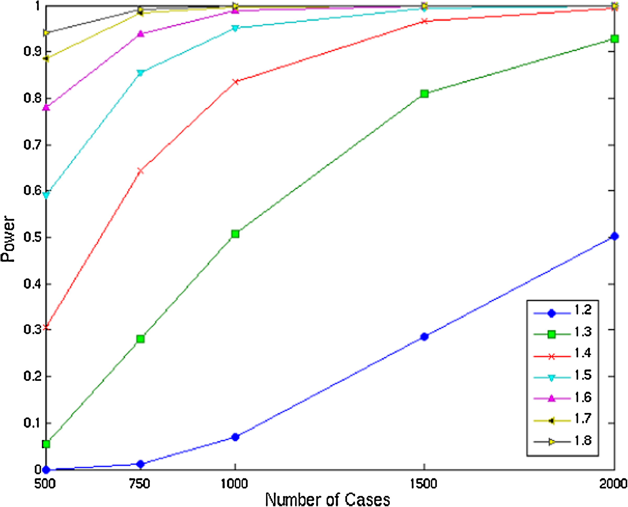
Statistical power of 4-marker window analysis under different disease models and sample sizes.

To evaluate the robustness of AAA to deviation from model assumptions, we examined the performance under inaccuracies in the admixture parameters. Namely, the inaccurate estimate λ of the number of generations since first admixture, and the inaccurate estimate of the ancestral distribution P(Q). Using a simulated population with African American admixture characteristics we conclude that the statistical power is insensitive (less than 1% decrease in power) to an inaccuracy of up to 5% in λ. Error in the estimate of P(Q) has a greater effect on power. In particular, a 5% overestimation of the contribution of the ancestry with the higher risk yields a 4.8% drop in power for a study with 2000 cases and ERR ≥ 1.5, and a 1.8% drop for a study with 1000 cases and ERR 1.8. When only 1000 cases are used to study a disease with a milder ERR of 1.5, the power drops significantly from 95% to 72%. The inaccuracies in the estimation of these admixture parameters are expected to be lower than 5% in the case of African Americans (Patterson et al., 2004).

To investigate the extent of genotyping reduction due to pooling we examined the number of SNP assays needed in order to achieve 70% power using our AAA method versus MALD. The MALD method performance was evaluated under the optimal condition where the ancestries are perfectly inferred by a fully informative single marker (see Section 2). The performance of AAA was examined over 2500 uniformly chosen locations along chromosome 1, using a window of four markers. In the case of AAA, we report the results under the configuration of k = 200 and l = 4, which resembles the choice of Sham et al. (2002) and Steer et al. (2006). The results are shown in Table 1. For ERR = 1.3, MALD requires a sample of 700 affected individuals, with one assay per individual. For the same disease model, AAA uses 28 assays, which suggests a 96% reduction in genotyping. The disadvantage of AAA is the need to collect additional affected individuals. However, for less than doubling the number of individuals, a 25-fold reduction in the number of assays is achieved. The performance of AAA was evaluated using a real panel for admixture mapping. When considering only perfect markers, AAA performance improves even when a single marker window analysis is applied, reducing the number of cases from 1300 to 1200, and the number of assays from 28 to 24. Similar results are obtained for ERR = 1.4.

Table 1.

Number of SNP Assays Needed to Achieve a Power of 70% Using MALD and AAA

	Cases		Assays
ERR	MALD	AAA	MALD	AAA
1.3	700	1300	700	28
1.4	470	820	470	20

The AAA method yields over 25-fold decrease in the number of SNP assays when using pool size k = 200 and number of replicates per pool l = 4.

ERR, ethnicity relative risk; MALD, mapping by admixture linkage disequilibrium; AA, admixture aberration analysis.

Table 2.

95^th Percentile of LOD Scores Using Pools of 500, 1000, and 2000 Simulated Controls Analyzed Using a Window of 2, 3, and 4 Markers Under the False Assumption of ERR between 1.3 and 1.8

	Two-markers window			Three-markers window			Four-markers window
Sample size	1.3	1.5	1.8	1.3	1.5	1.8	1.3	1.5	1.8
500	2.8	3.28	3.12	2.83	3.28	2.99	2.84	3.26	2.72
1000	3.29	3.14	1.72	3.3	2.89	0.78	3.28	2.75	0.26
2000	3.28	1.56	−1.78	3.06	0.65	−4.4	2.93	0.05	−6.39

All tested configurations exhibit a score lower than 3.3 in the 95^th percentile. The simulations demonstrate that in most cases an increase in either sample size or in the size of the sliding window results in a reduction of the threshold.

To evaluate the performance of AAA on real data, we examined a sample of 1646 African Americans with prostate cancer that were genotyped using 1985 ancestry informative SNPs. This sample led to the confirmation of prostate cancer risk locus in African American men through admixture mapping (Freedman et al., 2006). We simulated a pool using 600 cases that were genotyped with the same 1276 markers. The allele frequencies in the ancestral populations were estimated using a sample of 343 Europeans and 183 Africans. An ERR of 1.65 was used for the analysis based on Smith and O'Brien (2005). A European genetic contribution of 0.215 was estimated using a maximum likelihood approach on the pooled sample of affected admixed individuals.

Applying AAA using a window of four markers results in a significant signal near a known risk locus (for more details, see Fig. 4 in the Appendix). The peak on chromosome 8 (LOD 7.2) is less than 5Mb from the susceptibility locus reported by Freedman et al. (2006). Applying the AAA method genome-wide yielded two additional less significant signals on chromosomes 5 and 9 (LOD 3.7–3.8). To evaluate the robustness of the three significant signals, we applied AAA with four-marker and LOO filterring. The analysis shows that only the known locus on chromosome 8 persist, with a significant LOD of 5.88, while the other two peaks at chromosomes 5 and 9 drop to 0.2 and 1.46, respectively. We attribute the two additional signals to biased markers.

FIG. 4.

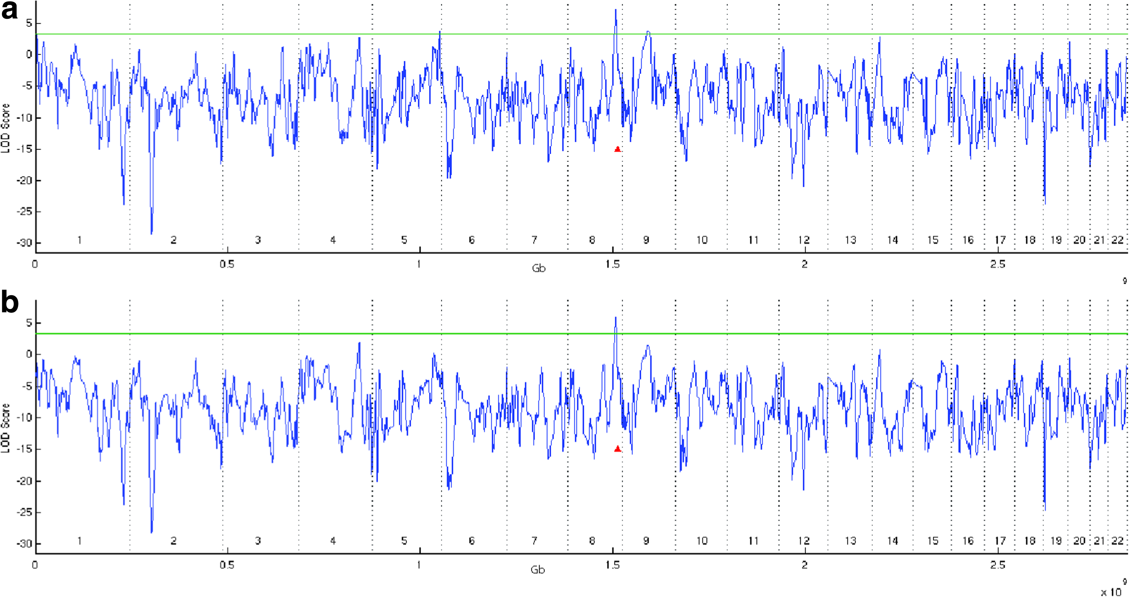
Analysis of 600 prostate cancer cases using AAA and a four-markers window. (a) The significant peak of 7.2 LOD is evident in close proximity to a validated prostate cancer risk locus at 129 Mb (marked by a triangle) that was previously discovered through a linkage scan by Amundadottir et al. (2006) and later reported by Freedman et al. (2006) using admixture mapping. Two additional significant signals are evident on chromosome 5 and 9. (b) Only the validated locus passes the LOO filter with a significant LOD of 5.88.

4. Conclusion

Pool-based methods rely on estimates of the allele frequencies in the pooled sample. It is known that pool-based association analysis is sensitive to errors in these estimates. Previous studies evaluated an error in the estimation of allele frequency difference between pools of less than 1.4% in 10K SNP arrays (Kirov et al., 2006). We now discuss the effects of these errors on AAA.

The model we used to simulate allele frequencies assumed independent normally distributed errors with zero mean. Three error levels were tested, adjusting the variance of the error so as to reflect a 95^th percentile of 1%, 3%, and 5% error in observed allele frequency. We performed simulations using pools of 500, 1000, and 2000 admixed controls, analyzing a window of 4 markers while using LOO filtering at 1cM steps, and assuming an ERR of 1.3–1.8. Each configuration was repeated 2500 times. The results are that the selected threshold of LOD = 3.3 is still valid for up to 5% error in allele frequencies for the case of ERR of 1.3–1.5 and 500–1000 affected individuals. These results further suggest that the analysis of the prostate cancer sample is robust to 5% allele frequency estimation error. Error in the estimation of allele frequencies has a greater impact on the false-positives rate in the case of a disease with a higher ERR or a larger sample, increasing the needed significance threshold defined by the 95^th percentile. One should adjust the significance threshold according to the expected allele frequency error via appropriate simulation.

We also repeated the experiment with cases, evaluating the impact of allele frequency estimation errors on the statistical power of AAA. The power of analyzing a disease with ERR of 1.5 using 1000 cases decreases from 95% to 82%. The tested error levels had a smaller effect on the analysis of a larger sample or a disease with a higher ERR value, still retaining a power of over 90%. In the analysis of a smaller sample size or a disease with a lower ERR, which achieved a power between 50% and 60% under accurate allele frequency estimation, the power decreased to 33–38% once such errors were introduced. However, in most of these settings, our simulated experiments on pooled controls suggest that a less stringent LOD threshold can be used without sacrificing the low level of false-positives.

The AAA method has an advantage over pooled association studies with respect to allele frequency estimation errors because (1) the aberration around the disease locus is supported by multiple markers, yielding a robust signal, (2) only a small fraction of SNP markers are required for the analysis, enabling the use of higher accuracy genotyping platforms, and (3) the ancestry informative markers are biased towards a high minor allele frequency in the admixed population, which increases the expected accuracy (Wilkening et al., 2007). The common enhancements applied in pool-based association studies of repeated measures and the subdivision of samples into pools should also increase the robustness of our method considerably.

Another source of error lies in the inaccurate estimation of allele frequencies of the ancestral populations which may lead to an increase in the number of false-positive signals. Indeed, initial experiments indicate that errors in the ancestral allele distribution increase the false-positive signals as these mimic the effect of a true risk allele. Such results may explain few of the additional suspected regions in the prostate cancer sample that were detected prior to applying LOO.

Our analysis assumes knowledge of the admixture coefficient P(Q), and the number of generations since the first admixture λ. While reasonable estimates of these parameters exists for some admixed populations, such as the African American and the Latino populations, it is recommended to tune the λ and P(Q) estimates using the sampled cases. We evaluated the genetic contribution of Europeans by applying a maximum likelihood approach on our prostate cancer cases pool, computing P(Q = Europe) = 0.215.

One of the properties of admixture mapping is that it can be applied on cases only, a property which holds for AAA as well. Nevertheless, similar to the use of control samples in MALD, healthy admixed individuals can increase the statistical power and decrease the rate of false-positives by providing a more accurate estimation of the allele frequencies in the ancestral population P(J|Q) as well as a more accurate estimation of the admixture parameters. Admixed controls pooled in several groups, each of similar admixture coefficient, can be used to adjust the estimates of ancestral allele frequencies using a maximum likelihood approach. In particular, measuring a marker's frequency in two African American control groups with a known and different admixture coefficient allows the estimation of the marker's frequencies in the ancestral populations via Equation 5.

The AAA method presented in Section 2 is developed for the case of an admixed population that was formed by two ancestral populations. Supporting admixed populations with more than two ancestral populations, as is the case with the Latino admixed population who are descendants of Native Americans, Europeans, and Africans, can be achieved through an adjustment of Equation 7. Another approach is to model all low risk populations as one ancestral population and the high risk population as the second ancestral population, applying the method as is.

Our multi-marker AAA method takes into account knowledge of linkage-disequilibrium evident in the ancestral population. Such inherent and complete incorporation of LD in the analysis further increases the method's statistical power, whereas other MALD methods do not fully benefit from this information, ranging from partial to no support of background LD. In addition, the analysis we developed is applied on a window of markers, while common MALD statistics employ an analysis of a single locus. Interestingly, the development steps presented in Section 2 imply that non-pooled MALD methods can also benefit from a multi-marker approach by deriving a statistic that evaluates aberration of inferred ancestries in a region, examining a range of marker locations rather than a single marker location at a time.

The goal of this work has been to alleviate the considerable cost of mapping. As the results indicate, a high power of 70% can be achieved for a disease with ethnicity prevalence differences comparable with end-stage kidney disease by pooling 1300 affected individuals, yielding a 25-fold reduction in genotyping in comparison to previous non-pooled MALD methods. We showed that AAA can be used by gene mapping groups as an economical, practical and powerful approach for the initial localization of regions containing disease genes.

5. Appendix

Footnotes

Acknowledgments

We thank Karl Skorecky for fruitful discussions on the MALD method. We are grateful to David Reich for providing the SNP readings from his prostate cancer study, which enabled the validation of the AAA method on real data. We thank Tamar Aizikowitz for her comments, as well as for help with our webpage design. S.B. is grateful to the Azrieli Foundation for the award of an Azrieli Fellowship. This research is partially supported by the Israel Science Foundation.

Disclosure Statement

No competing financial interests exist.

References

Amundadottir

L.T.

, Sulem

, Gudmundsson

et al. 2006. A common variant associated with prostate cancer in European and African populations. Nat. Genet, 38:652–658.

Arnheim

, Strange

, Erlich

1985. Use of pooled DNA samples to detect linkage disequilibrium of polymorphic restriction fragments and human disease: studies of the HLA class II loci. Proc. Natl. Acad. Sci. USA, 82:6970–6974.

Bercovici

, Geiger

2009. Inferring ancestries efficiently in admixed populations with linkage disequilibrium. J. Comput. Biol., 16:1141–1150.

Bercovici

, Geiger

, Shlush

et al. 2008. Panel construction for mapping in admixed populations via expected mutual information. Genome Res., 18:661–667.

Chakraborty

, Weiss

K.M.

1988. Admixture as a tool for finding linked genes and detecting that difference from allelic association between loci. Proc. Natl. Acad. Sci. USA, 85:9119–9123.

Darvasi

, Soller

1994. Selective DNA pooling for determination of linkage between a molecular marker and a quantitative trait locus. Genetics, 138:1365–1373.

Freedman

M.L.

, Haiman

C.A.

, Patterson

et al. 2006. Admixture mapping identifies 8q24 as a prostate cancer risk locus in African-American men. Proc. Natl. Acad. Sci. USA, 103:14068–14073.

Haiman

C.A.

, Patterson

, Freedman

M.L.

et al. 2007. Multiple regions within 8q24 independently affect risk for prostate cancer. Nat. Genet., 39:638–644.

Kao

W.H.L.

, Klag

M.J.

, Meoni

L.A.

et al. 2008. Myh9 is associated with nondiabetic end-stage renal disease in African Americans. Nat. Genet., 40:1185–1192.

10.

Kirov

, Nikolov

, Georgieva

et al. 2006. Pooled DNA genotyping on Affymetrix SNP genotyping arrays. BMC Genomics, 7:27.

11.

Long

J.C.

1991. The genetic structure of admixed populations. Genetics, 127:417–428.

12.

Patterson

, Hattangadi

, Lane

et al. 2004. Methods for high-density admixture mapping of disease genes. Am. J. Hum. Genet., 74:979–1000.

13.

Reich

, Patterson

2005. Will admixture mapping work to find disease genes? Philos. Trans. R. Soc. Lond. B Biol. Sci., 360:1605–1607.

14.

Rosenberg

N.A.

, Li

L.M.

, Ward

et al. 2003. Informativeness of genetic markers for inference of ancestry. Am. J. Hum. Genet., 73:1402–1422.

15.

Sham

, Bader

J.S.

, Craig

et al. 2002. DNA pooling: a tool for large-scale association studies. Nat. Rev. Genet., 3:862–871.

16.

Smith

M.W.

, O'Brien

S.J.

2005. Mapping by admixture linkage disequilibrium: advances, limitations and guidelines. Nat. Rev. Genet., 6:623–632.

17.

Smith

M.W.

, Patterson

, Lautenberger

J.A.

et al. 2004. A high-density admixture map for disease gene discovery in African Americans. Am. J. Hum. Genet., 74:1001–1013.

18.

Steer

, Abkevich

, Gutin

et al. 2006. Genomic DNA pooling for whole-genome association scans in complex disease: empirical demonstration of efficacy in rheumatoid arthritis. Genes Immun., 8:57–68.

19.

Tang

, Coram

, Wang

et al. 2006. Reconstructing genetic ancestry blocks in admixed individuals. Am. J. Hum. Genet., 79:1–12.

20.

The International HapMap Project. 2005. A haplotype map of the human genome. Nature, 437:1299–1320.

21.

The Wellcome Trust Case Control Consortium. 2007. Genome-wide association study of 14,000 cases of seven common diseases and 3,000 shared controls. Nature, 447:661–678.

22.

Wilkening

, Chen

, Wirtenberger

et al. 2007. Allelotyping of pooled DNA with 250k SNP microarrays. BMC Genomics, 8:77+.

23.

Zeng

, Lin

D.Y.

2005. Estimating haplotype-disease associations with pooled genotype data. Genet. Epidemiol., 28:70–82.