Towards Fully Automated Structure-Based NMR Resonance Assignment of 15 N-Labeled Proteins From Automatically Picked Peaks

Abstract

In NMR resonance assignment, an indispensable step in NMR protein studies, manually processed peaks from both N-labeled and C-labeled spectra are typically used as inputs. However, the use of homologous structures can allow one to use only N-labeled NMR data and avoid the added expense of using C-labeled data. We propose a novel integer programming framework for structure-based backbone resonance assignment using N-labeled data. The core consists of a pair of integer programming models: one for spin system forming and amino acid typing, and the other for backbone resonance assignment. The goal is to perform the assignment directly from spectra without any manual intervention via automatically picked peaks, which are much noisier than manually picked peaks, so methods must be error-tolerant. In the case of semi-automated/manually processed peak data, we compare our system with the Xiong-Pandurangan-Bailey-Kellogg's contact replacement (CR) method, which is the most error-tolerant method for structure-based resonance assignment. Our system, on average, reduces the error rate of the CR method by five folds on their data set. In addition, by using an iterative algorithm, our system has the added capability of using the NOESY data to correct assignment errors due to errors in predicting the amino acid and secondary structure type of each spin system. On a publicly available data set for human ubiquitin, where the typing accuracy is 83%, we achieve 91% accuracy, compared to the 59% accuracy obtained without correcting for such errors. In the case of automatically picked peaks, using assignment information from yeast ubiquitin, we achieve a fully automatic assignment with 97% accuracy. To our knowledge, this is the first system that can achieve fully automatic structure-based assignment directly from spectra. This has implications in NMR protein mutant studies, where the assignment step is repeated for each mutant.

1. Introduction

Nuclear magnetic resonance (NMR)-based technologies are not only important for determining protein structure in solution (Altieri and Byrd, 2004; Billeter et al., 2008), but also studying protein-protein, protein-ligand interactions (Mittermaier and Kay, 2006; Skinner and Laurence, 2008), and identifying new drugs (Pellecchia et al., 2008; Powers et al., 2008). However, presently, it can still take an experienced NMR spectroscopist weeks to months to process the data after the spectra are collected. A key bottleneck step in the data processing is backbone resonance assignment, where the goal is to assign chemical shift values extracted from the spectra to the underlying backbone atoms. Backbone resonance assignment generally requires some manual processing of peaks from both N-labeled and C-labeled spectra. In studies of wild-type and mutant peptides, the assignment step needs to be repeated for each peptide. Automated methods can accelerate this process especially if a similar 3D structure is already known, such as one obtained from a previous step. Previous steps will also yield assignment information. The additional data can allow subsequent steps to use only N-labeled NMR data without the added expense of C-labeled.

Traditional, sequence-based, resonance assignment methods depend mainly on the amino acid sequence and carbon connectivity information extracted from triple resonance experiments (Zimmerman et al., 1997; Güntert et al., 2000; Coggins and Zhou, 2003; Jung and Zweckstetter, 2004; Lemak et al., 2008; Alipanahi et al., 2009a). With the rate of new unique protein folds being discovered decreasing relative to the rate of protein structures being determined (Moult et al., 2005, 2007), one can expect that most proteins have homologs with a known protein structure. Analogous to molecular replacement in x-ray crystallography (Drenth, 2007), the known structure can be used as a template to which the NMR experimental evidence is matched, as is done in various structure-based assignment methods (Bartels et al., 1997; Bailey-Kellogg et al., 2000; Pristovsek et al., 2002; Hus et al., 2002; Erdmann and Rule, 2002; Langmead and Donald, 2004; Pristovsek and Franzoni, 2006; Xiong and Bailey-Kellogg, 2007; Xiong et al., 2008; Apaydin et al., 2008; Stratmann et al., 2009).

The nuclear vector replacement (NVR) approach (Langmead et al., 2004; Langmead and Donald, 2004) uses ¹⁵N-HSQC spectra, H^N-¹⁵N residual dipolar couplings (RDC), sparse unambiguous d_NN NOEs, amide exchange rates, and no triple resonance data for structure-based assignment. The problem was cast as a maximum bipartite matching problem, which they solved in polynomial time. Using close structural templates, they achieved an accuracy of over 99%. Their work was extended to handle more distant templates using normal mode analysis to obtain an ensemble of template structures (Apaydin et al., 2008). Unlike NOEs, which stem from short-range interactions, RDCs can provide long-range orientation information. However, currently in NMR labs, RDC experiments are not as commonly used for backbone resonance assignment. Very recently, the NVR approach was modified to use binary integer programming (Apaydin et al., 2010). Our approach, however, uses different data, and we directly model the relationship between pairs of residues with pairs of spin systems.

For assignment using 3D NOESY data, Xiong et al. developed a branch-and-bound algorithm (Xiong and Bailey-Kellogg, 2007), which they later improved to a randomized algorithm (Xiong et al., 2008), which we shall refer to as the contact replacement (CR) method. The CR method was demonstrated to tolerate 1–2Å structural variation, 250–600% noise, and 10–40% missing contact edges. Although they mention that there exists methods with close to 90% average accuracy for predicting a spin system's amino acid class prior to an assignment, the CR method ignored such errors. The method achieved an assignment accuracy of above 80% in α-helices, 70% in β-sheets, and 60% in loops. To our knowledge, it is the most error-tolerant structure-based assignment method in terms of the noise level. The data used consisted of only N-labeled spectra: 2D ¹⁵N-HSQC, 3D ¹⁵N-TOCSY-HSQC, 3D ¹⁵N-NOESY-HSQC, and ³J_HNHα coupling constants derived from 3D HNHA. The problem was cast as a subgraph matching problem, where one graph consisted of the contacts in the known protein structure, and the other consisted of the NOESY cross peaks (NOEs) that connected spin systems. In general, the mapping of NOESY peaks to specific contacts is ambiguous due to experimental errors, missing peaks, and false peaks. Although the graph problem that was solved is NP-hard in general, Xiong et al. proved that under their noise model, the problem could be solved in polynomial time with high probability.

In NOEnet (Stratmann et al., 2009), the problem was also cast as a subgraph matching problem. Unlike the CR method, NOEnet generates an ensemble of assignments containing all assignments compatible with the NMR data, and it requires only ¹H^N-¹H^N NOEs. However, it requires unambiguous NOEs, such as those from 4D NOESY experiments, so the noise is less than that handled by the CR method. NOEnet was recently updated to handle RDCs and chemical shifts from ¹⁵N-,¹³C-labeled proteins (Stratmann et al., 2010).

In NMR studies, NMR spectra are often examined by visual inspection, where the cross peaks get picked by inspection, or by automatic methods but then checked by the scientist to remove noisy peaks. The peaks get accumulated in a list of peaks, and this list can change during the study as errors and inconsistencies are discovered during the assignment step. Therefore, the peak picking and the resonance assignment steps are usually done together. We aim to build a system that automates this process without any manual intervention. The difficulty is that automatically picked peak lists are noisier than manually picked ones. To our knowledge, current structure-based methods are still semi-automated due to automated peak lists being of lower quality. The core of our system is a pair of integer programming models: one for predicting, a priori of a backbone assignment, the possible amino acid types and the ¹⁵N-TOCSY-HSQC peak corresponding to the Hα of each spin system; and the other model for backbone resonance assignment. As proof of concept, we solve this problem for automatically picked peaks from N-labeled only data, where related structure and assignment information is available. We perform an automatic assignment with accuracy 97% on a publicly available data set for ubiquitin. By accuracy we mean the number correct assignments over the number of assignments made by the system. Our automated peak picking system, PICKY (Alipanahi et al., 2009b), is used to pick the peaks.

To compare our system with existing methods, we consider processed peak data. In comparison with the CR method, on nine proteins from the simulated data set used by the CR method, our method, on average, has five times fewer incorrect assignments. This data set is in the form of a graph. As a step towards robust assignment, we achieve further error tolerance by using the NOESY data to directly handle errors in predicting each spin system's amino acid and secondary structure type. This was tested on five proteins with typing errors introduced, and also on manually picked peaks from the ubiquitin data set, where the combined type prediction accuracy is 83% (both amino acid and secondary structure type correct). On ubiquitin, we achieved an assignment accuracy of 91%, which is a large improvement over the 59% accuracy that was obtained without correcting for typing errors. Unlike the CR data set, the ubiquitin data set consisted of the spectra rather than a graph. We first describe our resonance assignment model that was compared with the CR method.

2. Methods

We use the graph representations from the CR method (Xiong et al., 2008) to represent the template protein of known structure and the NMR data of the unknown target protein. Please note that our integer linear programming formulation is independent of the details of their graph representation in that it can enforce constraints in a mathematical framework, while accomodating different sources of information.

Contact graph

Each residue in the template protein is represented by a vertex labelled with residue-related features. We use only amino acid and secondary structure type, but other residue-related features are possible. An edge is created between a pair of amino acids if there is a contact according to a given distance cutoff. Each edge is labelled by all pairs of directed proton-proton interaction types. We consider only two types of interactions, H^α and H^N, and H^N, and H^N. Since H^α and H^N is not symmetric, the labels have a direction.

Interaction graph

We define each spin system to consist of the chemical shifts of the backbone N, H^N, H^α, and the side chain protons. Each spin system is represented by a vertex labelled with spin system-related features. We use only the predicted amino acid and secondary structure type. Like the CR method, we use the side chain protons only in amino acid type prediction. Amino acid type predictions were obtained from the RESCUE software, version 1 (Pons and Delsuc, 1999). RESCUE classifies each spin system into one of ten possible amino acid classes using proton chemical shifts. We used all classes with positive reliability score rather than the highest scoring class to compensate for errors made by RESCUE. Secondary structure type predictions can be obtained from ³J_HNHα coupling constants (Wüthrich, 1986). An edge is created between a pair of spin systems if there is at least one matching NOESY peak (¹⁵N, H^N, ¹H), where the ¹⁵N, H^N matches the backbone N, H^N chemical shift of one spin system and the ¹H matches the backbone H^N or H^α of the other spin system. Edges are labelled similarly to the contact graph with the addition of a match score for each NOESY peak. The match score is defined as \documentclass{aastex}\usepackage{amsbsy}\usepackage{amsfonts}\usepackage{amssymb}\usepackage{bm}\usepackage{mathrsfs}\usepackage{pifont}\usepackage{stmaryrd}\usepackage{textcomp}\usepackage{portland,xspace}\usepackage{amsmath,amsxtra}\pagestyle{empty}\DeclareMathSizes{10}{9}{7}{6} \begin{document} $$er\,fc \Big( \frac { \mid \Delta e \mid } { 0.02 \times { \sqrt 2 } } \Big)$$ \end{document} as used in Xiong et al. (2008), where er fc is the complementary error function and \documentclass{aastex}\usepackage{amsbsy}\usepackage{amsfonts}\usepackage{amssymb}\usepackage{bm}\usepackage{mathrsfs}\usepackage{pifont}\usepackage{stmaryrd}\usepackage{textcomp}\usepackage{portland,xspace}\usepackage{amsmath,amsxtra}\pagestyle{empty}\DeclareMathSizes{10}{9}{7}{6} \begin{document} $$\mid \Delta e \mid$$ \end{document} is the chemical shift difference between ¹H and the matching H^N or H^α.

To find the best match between the two graphs, we look for the common edge subgraph that maximizes the match score, subject to the constraint that the vertex and edge labels match. Finding the maximum common weighted edge subgraph (and also the maximum common node subgraph), in general, is NP-hard (Raymond and Willett, 2002). We use integer programming to do the maximization because it models the problem naturally as we will show. Our ILP formulation is similar to that for the maximum clique problem (Bomze et al., 1999), to which subgraph matching can be reduced (Raymond and Willett, 2002). To solve the ILP model, we used the solver in the commercial optimization package ILOG CPLEX^®; version 9.130. Note that if we consider only vertex matches, we get a maximum bipartite matching problem, which can be solved in polynomial time as in the NVR method.

2.1. 0-1 Integer programming model

Define V_c, V_i to be the set of vertices in the contact graph and interaction graph, respectively. Define E_c, E_i to be the set of edges in the contact and interaction graph, respectively.

Input data

m(a, s, b, t) The edge match score between amino acids a, \documentclass{aastex}\usepackage{amsbsy}\usepackage{amsfonts}\usepackage{amssymb}\usepackage{bm}\usepackage{mathrsfs}\usepackage{pifont}\usepackage{stmaryrd}\usepackage{textcomp}\usepackage{portland,xspace}\usepackage{amsmath,amsxtra}\pagestyle{empty}\DeclareMathSizes{10}{9}{7}{6} \begin{document} $$b \in V_{c}$$ \end{document} and spin systems s, \documentclass{aastex}\usepackage{amsbsy}\usepackage{amsfonts}\usepackage{amssymb}\usepackage{bm}\usepackage{mathrsfs}\usepackage{pifont}\usepackage{stmaryrd}\usepackage{textcomp}\usepackage{portland,xspace}\usepackage{amsmath,amsxtra}\pagestyle{empty}\DeclareMathSizes{10}{9}{7}{6} \begin{document} $$t \in V_{i}$$ \end{document} , where a is matched with s, and b is matched with t. In our model, it is equal to the sum of the match scores of the NOESY peaks that match (s, t) and match an interaction type of (a, b). The score is assumed to be non-negative.

m(a, s) The vertex match score between amino acid a and spin system s. The score is assumed to be non-negative.

E_i(a, b) The set of edges in the interaction graph that match the edge \documentclass{aastex}\usepackage{amsbsy}\usepackage{amsfonts}\usepackage{amssymb}\usepackage{bm}\usepackage{mathrsfs}\usepackage{pifont}\usepackage{stmaryrd}\usepackage{textcomp}\usepackage{portland,xspace}\usepackage{amsmath,amsxtra}\pagestyle{empty}\DeclareMathSizes{10}{9}{7}{6} \begin{document} $$( a , \ b ) \in E_{c}$$ \end{document} . An edge \documentclass{aastex}\usepackage{amsbsy}\usepackage{amsfonts}\usepackage{amssymb}\usepackage{bm}\usepackage{mathrsfs}\usepackage{pifont}\usepackage{stmaryrd}\usepackage{textcomp}\usepackage{portland,xspace}\usepackage{amsmath,amsxtra}\pagestyle{empty}\DeclareMathSizes{10}{9}{7}{6} \begin{document} $$( s , \ t ) \in E_{i}$$ \end{document} matches edge (a, b) if the edge labels match, while taking into account the direction of the interaction, and if either the label of vertex a matches that of vertex s and the label of vertex b matches that of vertex t, or a with t and b with s.

A The set of all matching (a, s), where \documentclass{aastex}\usepackage{amsbsy}\usepackage{amsfonts}\usepackage{amssymb}\usepackage{bm}\usepackage{mathrsfs}\usepackage{pifont}\usepackage{stmaryrd}\usepackage{textcomp}\usepackage{portland,xspace}\usepackage{amsmath,amsxtra}\pagestyle{empty}\DeclareMathSizes{10}{9}{7}{6} \begin{document} $$a \in V_{c}$$ \end{document} and \documentclass{aastex}\usepackage{amsbsy}\usepackage{amsfonts}\usepackage{amssymb}\usepackage{bm}\usepackage{mathrsfs}\usepackage{pifont}\usepackage{stmaryrd}\usepackage{textcomp}\usepackage{portland,xspace}\usepackage{amsmath,amsxtra}\pagestyle{empty}\DeclareMathSizes{10}{9}{7}{6} \begin{document} $$s \in V_{i}$$ \end{document} , and there exists \documentclass{aastex}\usepackage{amsbsy}\usepackage{amsfonts}\usepackage{amssymb}\usepackage{bm}\usepackage{mathrsfs}\usepackage{pifont}\usepackage{stmaryrd}\usepackage{textcomp}\usepackage{portland,xspace}\usepackage{amsmath,amsxtra}\pagestyle{empty}\DeclareMathSizes{10}{9}{7}{6} \begin{document} $$( a , \ b ) \in E_{c}$$ \end{document} and \documentclass{aastex}\usepackage{amsbsy}\usepackage{amsfonts}\usepackage{amssymb}\usepackage{bm}\usepackage{mathrsfs}\usepackage{pifont}\usepackage{stmaryrd}\usepackage{textcomp}\usepackage{portland,xspace}\usepackage{amsmath,amsxtra}\pagestyle{empty}\DeclareMathSizes{10}{9}{7}{6} \begin{document} $$( s , \ t ) \in E_{i}$$ \end{document} such that (s, t) matches (a, b).

Decision variables

X(a, s, b, t) A binary variable. It equals to 1 if spin system s is assigned to amino acid a, and spin system t is assigned to amino acid b; and 0 otherwise. This variable represents an edge match between the graphs. X(b, t, a, s) is equivalent to X(a, s, b, t). For the purpose of exposition, we use X(a, s, b, t) to denote either X(b, t, a, s) or X(a, s, b, t), although the model contains only one such variable.

X(a, s) A binary variable. It equals to 1 if spin system s is assigned to the amino acid a; and 0 otherwise. This variable represents a vertex match.

Formulation
\documentclass{aastex}\usepackage{amsbsy}\usepackage{amsfonts}\usepackage{amssymb}\usepackage{bm}\usepackage{mathrsfs}\usepackage{pifont}\usepackage{stmaryrd}\usepackage{textcomp}\usepackage{portland,xspace}\usepackage{amsmath,amsxtra}\pagestyle{empty}\DeclareMathSizes{10}{9}{7}{6} \begin{document} \begin{align} \max_{X} & \left( \begin{matrix} \sum \limits_{ ( a , \ s ) \in A}m ( a , s ) \cdot X ( a , s ) + \\ \sum \limits_{ ( a , b ) \in E_{c}} \sum \limits_{ ( s , t ) \in E_{i} ( a , b ) }m ( a , s , b , t ) \cdot X ( a , s , b , t ) \end{matrix} \right) \tag{1} \end{align} \end{document} \documentclass{aastex}\usepackage{amsbsy}\usepackage{amsfonts}\usepackage{amssymb}\usepackage{bm}\usepackage{mathrsfs}\usepackage{pifont}\usepackage{stmaryrd}\usepackage{textcomp}\usepackage{portland,xspace}\usepackage{amsmath,amsxtra}\pagestyle{empty}\DeclareMathSizes{10}{9}{7}{6} \begin{document} \begin{align} \qquad \qquad subject \ to \\ & \qquad \sum_{s}X ( a , s ) \leq1 \quad \forall a \in V_{c} , \tag{2} \end{align} \end{document} \documentclass{aastex}\usepackage{amsbsy}\usepackage{amsfonts}\usepackage{amssymb}\usepackage{bm}\usepackage{mathrsfs}\usepackage{pifont}\usepackage{stmaryrd}\usepackage{textcomp}\usepackage{portland,xspace}\usepackage{amsmath,amsxtra}\pagestyle{empty}\DeclareMathSizes{10}{9}{7}{6} \begin{document} \begin{align} \qquad \sum_{a}X ( a , s ) \leq1 \quad \forall s \in V_{i} , \tag{3} \end{align} \end{document} \documentclass{aastex}\usepackage{amsbsy}\usepackage{amsfonts}\usepackage{amssymb}\usepackage{bm}\usepackage{mathrsfs}\usepackage{pifont}\usepackage{stmaryrd}\usepackage{textcomp}\usepackage{portland,xspace}\usepackage{amsmath,amsxtra}\pagestyle{empty}\DeclareMathSizes{10}{9}{7}{6} \begin{document} \begin{align} \quad \begin{matrix} \sum \limits_{t \ s.t. \ ( s , t ) \in E_{i} ( a , b ) }X ( a , s , b , t ) \leq X ( a , s ) \\ \forall ( a , s ) \in A , \; \forall ( a , b ) \in E_{c} \ , \end{matrix} \tag{4} \end{align} \end{document} \documentclass{aastex}\usepackage{amsbsy}\usepackage{amsfonts}\usepackage{amssymb}\usepackage{bm}\usepackage{mathrsfs}\usepackage{pifont}\usepackage{stmaryrd}\usepackage{textcomp}\usepackage{portland,xspace}\usepackage{amsmath,amsxtra}\pagestyle{empty}\DeclareMathSizes{10}{9}{7}{6} \begin{document} \begin{align} \quad X ( a , s , b , t ) \in \left\{ 0 , 1 \right\} \ , \tag{5} \end{align} \end{document} \documentclass{aastex}\usepackage{amsbsy}\usepackage{amsfonts}\usepackage{amssymb}\usepackage{bm}\usepackage{mathrsfs}\usepackage{pifont}\usepackage{stmaryrd}\usepackage{textcomp}\usepackage{portland,xspace}\usepackage{amsmath,amsxtra}\pagestyle{empty}\DeclareMathSizes{10}{9}{7}{6} \begin{document} \begin{align} \qquad X ( a , s ) \in \left\{ 0 , 1 \right\} \ . \tag{6} \end{align} \end{document}
Discussion

Equation (1), the objective function, expresses the total edge and vertex match score of the assignment. The first summation is over all vertices that are involved in at least one edge match. The second summation is over all edges that match. Unlike subgraph isomorphism, we look for edge matches only rather than non-matches. Non-matches are scored implicitly as described below. We generate only the variables involved in at least one edge match. We do not assign vertices that are isolated, unless the vertices can be unambiguously assigned, such as being the only ones with a particular type. Constraint (2) ensures that each amino acid is assigned to at most one spin system. Constraint (3) ensures that each spin system is assigned to at most one amino acid. Therefore, extra amino acids or spin systems can be unassigned, and missing amino acids or spin systems implicitly have a score of 0.

Constraint (4), in conjunction with (2) and (3), ensure that if X(a, s, b, t) = 1 , then X(a, s) = 1 and X(b, t) = 1. If X(a, s) = 1 and X(b, t) = 1, the left hand side of (4) can be zero, so missing edges are allowed. However, edge match scores are always non-negative and we are maximizing the score. If a match exists, we are guaranteed that one edge match variable is set to 1. Note that (2) and (3) prevent the situation in (4) where X(a, s, b, t) = 1 and X(a, u, b, v) = 1, or X(a, s, b, t) = 1 and X(i, s, j, t) = 1, so each contact graph edge has at most one matching interaction graph edge that gets picked, and vice versa. Since the interaction graph tends to have more edges than the contact graph, extra edges can get unmatched. Since edge match scores are non-negative, missing edges implicitly have a score of 0. The final two constraints ensure that the decision variables are binary. Note that the above formulation does not enforce that the common subgraph be connected, so contacts in different domains of the protein can get matched, while the parts in-between are unmatched.

2.2. ILP model generalizations

The ILP model can be adapted to accommodate different situations by setting, adding or removing variables, modifying their coefficients, and adding or removing constraints.

Different sources of data

Although we considered only chemical shift matches in the scoring function, the objective function of the ILP model can model any function that models the assignment of spins to residues and also the assignment of pairs of spins to pairs of residues. For C-labeled data, if there is carbon connectivity evidence that supports that spin systems s and t is associated with adjacent amino acids a_i and a_i₊₁, the value of m(a_i, s, a_i₊₁, t) can be increased. The variable X(a_i, s, a_i₊₁, t) can also be removed if there is insufficient connectivity and contact information.

For RDC data, once an alignment tensor has been estimated, back-computed RDCs can be computed and compared with the experimental values to yield a value for each m(a, s). After running the ILP, the assignment information can be used to update the alignment tensor and m(a, s) terms. For ¹H^N-¹H^N NOEs, chemical shift matches can be encoded in the m(a, s, b, t) terms.

Different weights on m(a, s, b, t) can be used to account for matches to specific types of contacts in the template protein structure, such as long range β-sheet contacts and local H^α and H^N contacts in α-helices. The CR method focused on finding common Hamiltonian path fragments in the graphs to be matched. Similar to carbon connectivity, the score for matches to pairs of adjacent amino acids can be scaled up to emphasize the Hamiltonian path, so that the objective function contains a weighted version of the Hamiltonian path length.

Note that if we remove the X(a, s, b, t) variables, and consider only the X(a, s) variables and use dummy vertices in the case that the size of V_c is not equal to V_i, we get a maximum bipartite matching problem. In this case, we can relax the constraint that the variables are integers because the constraint matrix becomes totally unimodular (Burkard et al., 2009), so linear programming, which is not NP-hard, will give an integer optimal solution.

A priori assignment information

ILP solvers can start from an initial solution to improve performance. This initial solution can even be a partial assignment. If specific spin system-amino acid assignments are known, the corresponding vertex match variables can be fixed to 1. The ability to fix specific assignments and to start from an existing assignment allows for a semi-automated approach, where the returned assignment is examined and corrected manually. The ILP can then be rerun using the new information rather than starting from scratch.

Multiple solutions

The maximum common subgraph is not necessarily unique, so there may be multiple best scoring assignments. The sequential algorithm, introduced by Greisdorfer et al. (2008) and generalized to more than two solutions in Danna et al. (2007), can be used to generate solutions that are guaranteed to be within a certain percentage of the optimal solution and have maximum diversity as measured by a diversity measure, such as average pairwise hamming distance. The one tree algorithm can also be used (Danna et al., 2007). Examining the variability of each amino acid's possible assignments among a set of optimal or near optimal assignments allows one to assess the assignment stability. The set of assignments can be used in consensus methods. For instance, the above ILP can be used to generate a consensus assignment by ignoring the X(a, s, b, t) variables and setting each m(a, s) to the number of times amino acid a is assigned to spin system s.

2.3. Spin system type prediction errors

In the current ILP model, an edge match requires that the corresponding vertices match in amino acid and secondary structure type. If there are type prediction errors, there will be assignment errors. To correct for these errors, after solving the ILP with the type matching requirement, we identify putative correct assignments and relax the type matching requirement for the remaining residues. The ILP is then resolved with the fixed assignments. Our approach to handle type prediction errors is summarized in Figure 1.

FIG. 1.
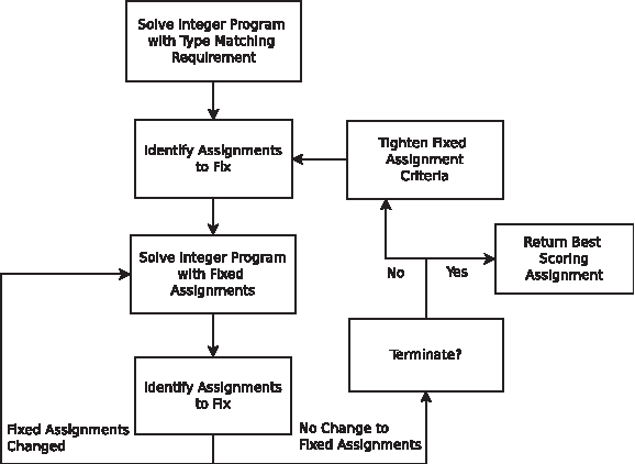
Iterative integer programming with fixed assignments.

To determine whether or not an assignment should be fixed, we examine the percentage of contacts matched involving each assigned amino acid. This percentage can be outputted as a confidence measure for each assignment. Due to erroneous assignments, an overly tight criteria for identifying fixed assignments may exclude many correct assignments and result in a large problem size. For the initial criteria, we chose a 50% cutoff, and then we used progressively tighter criteria. Once the ILP is resolved, the previously fixed assignments may no longer satisfy the criteria, while new assignments may satisfy it. Therefore, for a given criteria, we resolve the ILP until the fixed assignments do not change, or after a maximum number of iterations. From our tests, the number of iterations did not exceed 5. We chose 50% because the majority of the missing edge percentages in our data are below 50% (Table 1). To tighten the criteria, we considered the requirement that a certain number of sequential neighboring contacts, nonlocal contacts between β-sheet amino acids, and local helix contacts (i ± 5) in the template protein structure be matched. We first required only one sequential neighbor and then later two (assignments for amino acids at the end points will not be fixed). Finally, we required that β-sheet amino acids have at least one β-sheet contact match, and that α-helix amino acids have at least one local contact match before and one local contact match after the residue. We did not attempt to optimize the set of criteria for fixing assignments as this is a modeling issue, and we wanted to show that our ILP model is flexible in modeling the problem.

Table 1.
Summary of the Test Set

Template No. residues No. spin sys No. PRO Noise (×) Missing (%) RMSD (Å)

1KA5 88/40/23/25 85/39/23/23 1 5.5/5.6/5.9/5.3 21/20/21/22 0.2/0.2/0.1/0.2

1EGO 85/40/19/26 81/40/19/22 3 5.6/5.4/5.8/6.3 22/22/26/19 1.6/1.4/0.9/2.3

1G6J 76/18/22/36 72/18/22/32 3 4.4/3.5/5.1/4.8 33/31/32/35 1.1/0.6/0.4/1.5

1SGO 139/46/28/65 136/46/28/61 3 5.5/4.7/4.0/7.4 41/38/49/40 10.9/7.3/5.5/14.1

1YYC 174/36/72/66 158/36/70/52 10 6.6/5.2/7.5/7.3 38/35/38/40 4.0/2.5/1.6/6.0

2NBT 66/-/16/50 60/-/16/48 5 3.4/-/3.6/3.3 36/-/22/40 3.4/-/1.7/3.8

1RYJ 70/9/27/34 67/9/27/31 2 3.1/2.0/3.1/3.8 28/33/29/25 1.5/1.0/0.9/1.9

2FB7 80/-/32/48 73/-/32/41 7 3.1/-/3.0/3.2 34/-/30/36 5.4/-/2.0/6.8

1P4W 87/66/-/21 82/65/-/17 3 5.5/5.3/-/6.7 31/28/-/40 1.1/0.7/-/1.9

From left to right: template structure, number of residues in the template (total/helix/sheet/loop); number of spin systems (total/helix/sheet/loop); number of prolines; noise level (number NOE edges per contact); percentage of contacts missing in the NMR data (total/helix/sheet/loop); average pairwise RMSD of the models in the template PDB file (total/helix/sheet/loop).

Since a fixed assignment can be incorrect, we generate multiple assignments and then identify fixed assignments in each assignment in order to produce different fixed assignments. For a given fixed assignment criteria, this results in a set of solutions. The best scoring assignment is then taken as the starting point for the next fixed assignment criteria. Previous assignments can be supplied to CPLEX as an initial feasible solution to speed up the optimization. To examine the possible assignments for the non-fixed residues, multiple solutions can be generated from the final assignment by fixing assignments and then running the sequential or one tree algorithm.

For a given fixed assignment, ILP solvers can return a solution with score guaranteed to be at most N% away from the optimal score, where we chose N to be 1%. Due to noisy edges, increased ambiguity from relaxing the type matching requirement, incorrect fixed assignments, and inaccuracies in the scoring function in modeling the problem, the solution with the optimal score is not necessarily the correct solution. Nevertheless, from our tests, we found that the score of the correct assignment is near the optimal.

3. Results

We tested the performance of our method on the synthetic data set used by the CR method. It consisted of nine proteins. The authors provided us with simulated data, in the form of an interaction graph, that was derived from the following NMR structures from the PDB: 1KA5, 1EGO, 1G6J, 1SGO, and 1YYC. The data for the other four proteins were simulated according to their simulation method described in Xiong and Bailey-Kellogg (2007), where only one of the NMR models was used to generate the NOESY peaks. Although the simulated data was derived from one of the models in the PDB file, similar to the CR experiments, we tested the data using every model in the PDB file as the template structure, where the number of models per PDB file ranged from 10 to 32. The structural noise (in RMSD) of the models within each PDB file is given in Table 1, which summarizes the test set. To control noise, our method automatically increases the distance cutoff at 0.25 Å increments until the noise level is under 8. This gives an improvement over using a fixed 4 Å cutoff. We used the same distance cutoffs in the CR software.

Table 2 compares our method with the CR method, where the first row of each entry gives our results, while the row below gives the CR's. On eight of the nine proteins, our average accuracy on the entire protein is better. We achieved an average accuracy of 97.1%, whereas the CR method has 86.0% accuracy, resulting in 4.8 times fewer wrong assignments by our method. We also noticed that the ILP model significantly outperforms the CR method on both β-sheet and loop regions. This may be due to the fact that our method can maximize the score better as shown in column 4 of Table 2. In many instances, the score is higher than the score of the correct assignment, which indicates that maximizing contact matches alone may not necessarily give the correct assignment. For 2NBT, where 40% of loop contacts are missing, we did slightly worse, but the score is greater than the score of the correct assignment; similarly for helix residues in 1RYJ. In general, since amino acids in helices tend to have local contacts with nearby amino acids, in many of our tests, we observed that missing NOE edges and typing errors produced local errors in helices. For 1RYJ, the accuracy for helices using a (i ± 2) window, i.e., allowing a spin system to be assigned within two residues away from the correct residue, is 100%.

Table 2.
Comparison Between the ILP Model and the Contact Replacement Method for Correct Amino Acid and Secondary Structure Typing

Template Avg. acc. (%) Acc. range (%) Times score [>,<, = Ref]

1KA5 100/100/100/100 100/100/100 0, 0, 16

94/100/76/100 98-93/91-74/100 0, 16, 0

1EGO 98/100/100/93 100-97/100/100/100-90 15, 0, 5

96/96/100/93 100-92/100-90/100/100-79 4, 12, 4

1G6J 97/100/100/94 100-95/100/100/100-90 25, 2, 5

91/100/ 87/88 97-89/100/100-86/100-85 0, 32, 0

1SGO 96/97/100/94 100-86/100-95/100/100-70 13, 3, 4

80/95/95/62 88-71/100-87/100-86/76-45 0, 20, 0

1YYC 97/99/96/98 100-93/100/100-91/100-92 17, 0, 3

72/92/62/72 76-67/100-89/69-53/79-64 0, 20, 0

2NBT 91/-/98/88 96-85/-/100-93/95-79 10, 0, 0

92/-/95/90 100-88/-/100-88/96-82 1, 9, 0

1RYJ 97/98/96/96 97-94/100-88/96/96-93 20, 0, 0

82/100/70/86 82-75/100/70/88-72 0, 20, 0

2FB7 96/-/97/96 100-91/-/100-93/100-90 7, 0, 3

92/-/94/90 95-88/-/100-94/95-83 0, 10, 0

1P4W 99/100/-/97 100-97/100/-/100-88 4, 0, 16

77/77/-/77 91-63/91-63/-/90-58 0, 20, 0

Average 97/99/99/96 — —

86/94/85/84 — —

For each protein, the first row gives our results, while the second row gives the CR's. From left to right: template structure; average accuracy over all the models (total/helix/sheet/loop); accuracy ranges (total/helix/sheet/loop); number of times the assignment score was greater than, less than, or equal to the score of the correct assignment.

The CR software did not allow for the input of amino acid and secondary structure type predictions, so we could only perform the comparison assuming correct amino acid and correct secondary structure typing. Nevertheless, since perfect spin system typing cannot be achieved easily, we also tested our method on predicted spin system types. First we tested with only amino acid type prediction, and then we tested with both amino acid and secondary structure typing errors. For the five data sets received, we ran RESCUE Version 1 (Pons and Delsuc, 1999) on the experimental proton chemical shifts from the protein's entry in the Biological Magnetic Resonance Bank (BMRB) (Ulrich et al., 2008). Table 3 gives the results with amino acid type prediction. For comparison, we included the results of using type matching as strict constraints; that is, the result without using the iterative algorithm that tries to correct for typing errors. In general, type correction resulted in large improvements. For 1G6J, the amino acid typing accuracy is high, so the improvement is minimal. For 1YYC, the improvement is significant even though the typing accuracy is low. The accuracy, however, varied substantially depending on the model used as the template. Nevertheless, the template with the best score yielded an accuracy of 89.9%, which increases to 94.1% when considering an (i ± 2) window. This indicates that using multiple templates, such as those generated by normal mode analysis (Apaydin et al., 2008), may improve accuracy. In these tests, we used weaker criteria for fixing assignments. We did not require nonlocal β-beta sheet and local α-helix contact matches.

Table 3.
Assignment Accuracy for Amino Acid Typing Errors and Correct Secondary Structure Typing

Template Avg. acc. strict. (%) Avg. acc. iter. (%) Range acc. iter. (%) A.A. typing acc. (%) Times score [>, <, = Ref]

1KA5 86 100/100/100/100 100/100/100/100 89 0, 0, 16

1EGO 86 94/92(99)/100/94 100-91/100-87/100/100-90 90 15, 3, 2

1G6J 92 94/100/93/91 97-87/100/100-90/100-78 96 7, 25, 0

1SGO 82 92/90(100)/95/93 96-87/100-84/100-82/96-83 92 7, 13, 0

1YYC 59 77/86 (92)/81/66 94-68/100-58/100-52/90-50 79 0, 20, 0

From left to right: template structure; average accuracy for strict type matching; average accuracy for iterative error correction over all the models (total/helix/sheet/loop); accuracy ranges for iterative error correction (total/helix/sheet/loop); amino acid typing accuracy; number of times the assignment score was greater than, less than, or equal to the score of the correct assignment. Values in parenthesis give the accuracy within an i ± 2 window.

Table 4 gives the results for both amino acid and secondary structure typing errors. The standard method for predicting secondary structures from ³J_HNHα coupling constants (Wüthrich, 1986) is similar to the following: if the coupling value is between 2.5 and 5.5, the spin system is predicted as helix. If the value is between 8 and 11.5, the spin system is predicted as β-sheet; otherwise, it is predicted as loop. From a test set of the following BMRB entries with accession numbers 4267, 4071, 2151, 4458, 4376, 4136, 4784, 4347, 4163, 4297, plus ubiquitin experimental values from the literature (Wang and Bax, 1996), we obtained an average typing accuracy of 60% with a range of 50–69%. This will likely be too low for resonance assignment, so we classified coupling constants into classes consisting of two secondary structure types, which dramatically increased the average accuracy at the cost of increased problem size and increased ambiguity. For values less than 6.5, we classify it as helix and loop; otherwise, we classify it as β-sheet and loop. With this, we obtained an average accuracy of 92% with a range of 82–100%.

Table 4.
Assignment Accuracy for Both Amino Acid and Secondary Structure Typing Errors

Template Acc. strict. (%) Acc. best score iter. (%) A.A. typing acc. (%) S.S. typing acc. (%) Diff ref. score (%)

1KA5 72 100/100/100/100 89 91 0

1EGO 65 97/95(100)/100/100 90 85 −1.5%

1SGO 63 88/82(91)/96/88 92 87 −3.0%

1G6J 75 91/100/86/90 96 90 +0.5%

1YYC 40 70/91/71/53 79 91 −3.1%

From left to right: template structure; accuracy for strict type matching; accuracy of the best scoring model for iterative error correction (total/helix/sheet/loop); amino acid typing accuracy; secondary structure typing accuracy; percentage difference in score of the best scoring assignment compared to the correct one (+means score of our assignment was higher). Values in parenthesis gives the accuracy in a (i ± 2) window.

For our tests, we introduced secondary structure class prediction errors yielding the typing accuracies in Table 4, which are below 92%. In these tests, we used the nonlocal β-beta sheet and local α-helix contact match criteria for fixing assignments. For the convenience of time, we tested each target using only the first model in the template. The noise level and percentage of missing NOEs is similar to the average values in Table 1. From column 2 of Table 4, we see that low assignment accuracies can result if spin system type prediction errors are not handled, even if the type prediction accuracy is high. For 1KA5, the assignment accuracy did not change from the previous test. For 1EGO, the accuracy actually improved because of the tighter criteria for fixing assignments. The larger 1SGO struggled to maximize the score, but the accuracy is still much higher than without the iterative algorithm. For 1YYC, its large size combined with its low amino acid typing accuracy, produced poor quality fixed assignments, but there is still a large improvement over the case without the iterative algorithm.

For ubiquitin, which is a commonly used protein to test resonance assignment methods, we obtained ¹⁵N HSQC, ¹⁵N TOCSY-HSQC, and ¹⁵N NOESY-HSQC data from Richard Harris's The Ubiquitin Resource Page (Harris). In this test, we are using experimentally derived spectra rather than simulated data. We picked the peaks manually by inspecting the spectra with SPARKY (Goddard and Kneller). Ubiquitin has 76 residues and three prolines. The reference solution has 70 assigned residues. The noise level is 4.6 at 4 Å cutoff, and the missing edge percentage is 28.3%. HSQC peaks without an H^α chemical shift were correctly filtered out as noise. For amino acid typing, RESCUE performed poorly, giving an accuracy of 68.6%. The errors appear to be due to missing peaks that are hidden by peak overlap. Using a higher resolution TOCSY spectrum may improve accuracy. We performed the typing manually using each type's expected number of proton chemical shifts and their expected range of values. Manual typing gave an accuracy of 90%, where the average number of possible amino acid types per spin system is 3.3, with a range of 1–8. We used the results of manual typing for assignment. RESCUE version 2 (Marin et al., 2004) yielded an accuracy of 90% as well, but only after the peaks were manually assigned to their spin systems. Since we manually picked the peaks, we might as well perform the type prediction at the same time.

We used experimental ³J_HNHα coupling constants from the literature (Wang and Bax, 1996). Eight spin systems did not have J-coupling values, so their predicted class included all three secondary structure types. The accuracy of secondary structure type prediction was 91%, yielding a combined typing accuracy of 83%. Model 1 from PDB 1D3Z was used as the template structure. The template structure was not derived from the NMR data. An NMR model was used to test the case of using results from previous NMR studies. The best scoring assignment had accuracy 87.1%, with 64.3% on α-helix (85.7% with i ± 2 window), 95.7% on β-sheet, and 90.0% on loops. Although the accuracy for helix residues is low, many of the errors are due to a ±1 assignment position error due to the HSQC peak of a nearby amino acid not being present in the NMR data. We also obtained a consensus assignment by generating 10 solutions from the best scoring assignment with fixed assignments meeting the secondary structure contact matching criteria. Consensus gave an accuracy of 91% (62 out of 68 predictions) with 78% for helices (92% i ± 2) and the other types unchanged. This result from a non-synthetic data set is comparable to the result for the 1G6J synthetic data set, which is also ubiquitin, except that this test is slightly more difficult. This data set is missing HSQC peaks for two residues in addition to proline residues, which are known not to have HSQC peaks. The synthetic data set is missing only prolines and the initial methionine, which is also known not to have an HSQC peak. Without the iterative algorithm, the accuracy is 59%.

4. Fully Automated Assignment from Automatically Picked Peaks

For this problem, we used only three spectra—¹⁵N HSQC, ¹⁵N NOESY-HSQC, and ¹⁵N TOCSY-HSQC—from The Ubiquitin Resource Page. To simplify the problem, J-coupling constants were not used. These values do not seem to be commonly available in the BMRB, especially for large proteins. In general, obtaining a high yield of J-coupling constants from HNHA becomes more difficult as the protein size increases. Instead of using secondary structure type predictions, we used related assignment information, which is typically available in NMR protein mutant studies. Although our approach is automated, it estimates some parameters that likely would be better estimated by a quick visual inspection of the data, such as intensity cutoffs for noisy peak removal. Figure 2 summarizes our approach. Peaks are first picked from the spectra, and then the peak lists are calibrated and noise filtered. The peaks are then grouped into spin systems, which, in turn, get type predicted. Finally, the graphs for resonance assignment are built, followed by the assignment step. The details of each step follows.

FIG. 2.
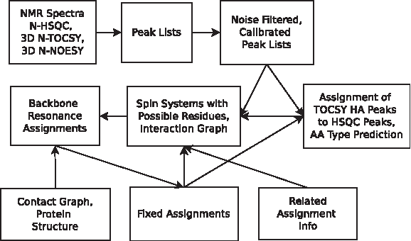
Automated backbone resonance assignment with protein structure and related assignment information. Arrows denote the flow of information, starting from the NMR spectra. Note that the backbone resonance assignment step is iterative. Fixed assignments are used to reduce the set of possible residues and to limit type prediction to only the unfixed spin systems.

4.1. Peak picking and peak list processing

Peak lists were obtained using PICKY, and then they were calibrated to align the N, H^N of the TOCSY and NOESY peaks to those in the HSQC. To maximize the number of N, H^N matches, we modeled calibration as a maximum clique problem on the intersection graph of rectangles, which can be solved in O(nlogn) time (Imai and Asano, 1983). We used rectangles with widths corresponding to the typical match tolerances of 0.5 ppm and 0.05 ppm, respectively, for the N and H^N dimensions of each HSQC peak. For the TOCSY/NOESY peaks, whose N and H^N coordinates are altered, we used a 0.5 ppm, 0.05 ppm rectangle as the search space, but this can be adjusted. To remove the influence of noisy peaks, we used only the top 50% most intense peaks to determine the N and H^Noffsets. The NOESY H was also calibrated against the TOCSY H by matching as many protons as possible. This was done by solving a maximum clique problem on the intersection graph of intervals, which can be solved in linear time (Möhring, 1986). Each TOCSY and NOESY H was represented by a 0.05 ppm interval centered about the peak. For ubiquitin, if calibration is not performed, the missing edge percentage increases by 12%. The combination of automated peak picking and peak list calibration resulted in a missing edge percentage of 36–45% (see Section 4.3). This is much higher than using manually picked peaks, which indicates that there is room for improvement in our peak picking and peak list calibration method. In general, peak picking is a non-trivial problem and an urgent target for improvement (Williamson and Craven, 2009).

When using automatically picked peaks, a true peak may have other nearby noisy peaks of similar chemical shift value, but of lower intensity. For the 3D spectra, overlapped peaks within 0.5, 0.05, 0.05 ppm were merged, and only the peak with the higher intensity was kept. Noisy HSQC peaks were identified by sorting the peaks by intensity, and then using a 4-SD cutoff to remove low intensity peaks.

To identify which TOCSY peaks should be grouped together, we used a divisive hierachical clustering approach. We first grouped TOCSY peaks into strips where all peaks in a strip matched at least one HSQC peak within a 0.5, 0.05 ppm tolerance and are within 0.5, 0.05 ppm of each other. TOCSY peaks not in any strips were removed. Strips may correspond to putative side chain protons of a given residue. A peak can occur in more than one strip due to peak overlap. To split strips, the 4 corners of each strip was defined by the maximum, minimum N and maximum, minimum H^N chemical shift values of the peaks in the strip. Peaks were then assigned to the closest corner. If there were groups of size at least 2 (since we want each strip to have H^N and Hα), and the difference in the assigned corners of the groups was larger than 0.25 ppm for N or 0.025 ppm for H^N, the strip was split. Using statistics from the BMRB, strips with no H^N and putative Hα atoms were removed. For instance, Hα's typically have chemical shift values of 2–6.

Noisy TOCSY peaks in each strip were removed by intensity using an approach similar to the one used for HSQC peaks. NOESY peaks were matched to HSQC peaks using a 0.5, 0.05 ppm tolerance. Noisy NOESY peaks were identified in a later step (see Section 4.3). Since the removal of peaks may change calibration, calibration and peak list processing was repeated until no additional peaks were removed. It is known that peak list processing can have a significant impact on assignment accuracy (Pawley et al., 2005).

The processed HSQC and TOCSY peaks were passed to the amino acid typing and Hα assignment module. After processing, the number of HSQC peaks was 84 versus 90 in the initial peak list. The initial TOCSY peak list had 2019 peaks, while the processed one had 311. The initial NOESY peak list had 1552 peaks, while the processed one had 287 (see Section 4.3).

4.2. Amino acid type predicton and Hα assignment

Our ILP for resonance assignment requires, as input, a list of possible amino acid types for each HSQC peak, and the TOCSY peaks representing the Hα atoms of the residue that is represented by the HSQC peak. In RESCUE 2, the grouping of TOCSY peaks to their corresponding HSQC peak, known as TOCSY assignment, is assumed to be known a priori of type prediction. We extended the Bayesian scoring model in RESCUE 2 to perform both type prediction and TOCSY assignment. Unlike the side chain resonance assignment problem, we do not have an a priori backbone assignment, so we can obtain only a distribution of assignments. For our problem, we considered only the distribution of TOCSY assignments to Hα's. To our knowledge, we are not aware of any other system that can perform amino acid type prediction and Hα prediction simultaneously from chemical shift information without an a priori backbone assignment.

To obtain the amino acid type predictions, we sampled the probability distribution of X , which is the set of (i, R), where the residue represented by HSQC peak i is assigned to amino acid type R. Letting H represent the set of HSQC peaks and T represent the TOCSY peaks, and applying Bayes' rule, we have \documentclass{aastex}\usepackage{amsbsy}\usepackage{amsfonts}\usepackage{amssymb}\usepackage{bm}\usepackage{mathrsfs}\usepackage{pifont}\usepackage{stmaryrd}\usepackage{textcomp}\usepackage{portland,xspace}\usepackage{amsmath,amsxtra}\pagestyle{empty}\DeclareMathSizes{10}{9}{7}{6} \begin{document} \begin{align} P (\textbf {\textit {X}} \ \mid \ \textbf {\textit {H}} , \ \textbf {\textit {T}}) &= \sum_ {\textbf {\textit {Z}}} P (\textbf {\textit {Z}} , \ \textbf {\textit {X}} \ \mid \ \textbf {\textit {H}} , \ \textbf {\textit {T}}) \\ &= \frac {1} {P (\textbf {\textit {H}} , \ \textbf {\textit {T}})} \sum_ {\textbf {\textit {Z}}} P ( \textbf {\textit {Z}} , \ \textbf { \textit {X}} , \ \textbf {\textit {H}} , \ \textbf {\textit {T}}) \\ &= \alpha \sum_ {\textbf {\textit {Z}}} \left (P (\textbf {\textit {T \ }} \mid \ \textbf {\textit { H } } , \ \textbf {\textit {Z}} , \textbf {\textit {\ X}}) \times P (\textbf {\textit {H}} \ \mid \ \textbf {\textit {Z}} , \textbf {\textit {\ X}}) \times P (\textbf {\textit {Z}} \ \mid \ \textbf {\textit {X}}) \times P (\textbf {\textit {X}}) \right ) ( 7 ) \end{align} \end{document}

where α is a normalization constant to denote P( H, T ), which is related to the input peak lists, and Z is the set of assignments ( A , M , N ) that are defined below.

Each HSQC peak i is represented by its N and H^N chemical shift values, which we denote collectively by δ_i. We allow HSQC peaks to have no amino acid type assignment. Each TOCSY peak j is presented by its N, H^N, H chemical shift values, which we denote collectively by δ_j, and by the peak intensity value denoted by I_j. Each TOCSY peak j can be assigned as noise or to a proton R_k of an amino acid of type R. Each R_k can be assigned to a TOCSY peak j or be assigned as being missing its TOCSY peak. Letting \documentclass{aastex}\usepackage{amsbsy}\usepackage{amsfonts}\usepackage{amssymb}\usepackage{bm}\usepackage{mathrsfs}\usepackage{pifont}\usepackage{stmaryrd}\usepackage{textcomp}\usepackage{portland,xspace}\usepackage{amsmath,amsxtra}\pagestyle{empty}\DeclareMathSizes{10}{9}{7}{6} \begin{document} $$( i , \ j , \ R_{k} ) \in\textbf{\textit{A}}$$ \end{document} denote an assignment of TOCSY peak j to proton R_k of some residue represented by HSQC peak i, letting \documentclass{aastex}\usepackage{amsbsy}\usepackage{amsfonts}\usepackage{amssymb}\usepackage{bm}\usepackage{mathrsfs}\usepackage{pifont}\usepackage{stmaryrd}\usepackage{textcomp}\usepackage{portland,xspace}\usepackage{amsmath,amsxtra}\pagestyle{empty}\DeclareMathSizes{10}{9}{7}{6} \begin{document} $$( i , \ R_{k} ) \in\textbf{\textit{M}}$$ \end{document} denote proton R_k assigned to HSQC peak i and missing its TOCSY peak, and letting \documentclass{aastex}\usepackage{amsbsy}\usepackage{amsfonts}\usepackage{amssymb}\usepackage{bm}\usepackage{mathrsfs}\usepackage{pifont}\usepackage{stmaryrd}\usepackage{textcomp}\usepackage{portland,xspace}\usepackage{amsmath,amsxtra}\pagestyle{empty}\DeclareMathSizes{10}{9}{7}{6} \begin{document} $$j \in\textbf{\textit{N}}$$ \end{document} denote TOCSY peak j assigned to noise, we can expand Equation 7 to give \documentclass{aastex}\usepackage{amsbsy}\usepackage{amsfonts}\usepackage{amssymb}\usepackage{bm}\usepackage{mathrsfs}\usepackage{pifont}\usepackage{stmaryrd}\usepackage{textcomp}\usepackage{portland,xspace}\usepackage{amsmath,amsxtra}\pagestyle{empty}\DeclareMathSizes{10}{9}{7}{6} \begin{document} \begin{align} &\sum_{(\textbf{\textit{A}} , \textbf{\textit{M}} , \textbf{\textit{N}})} \bigg( \Big( P \big( \textbf{\textit{T}}_A \ | \ \textbf{\textit{A}} , \ \textbf{\textit{X}}_A \big) \times P \big( \textbf{\textit{A}} \ | \ \textbf{\textit{X}}_A \big) \Big) \times P \big( \textbf{\textit{M}} \ | \ \textbf{\textit{X}}_{M} \big) \times \big( P (\textbf{\textit{T}}_{N} \ | \ \textbf{\textit{N}} ) \times P ( \textbf{\textit{N}} ) \big) \times \big( P ( \textbf{\textit{H}} \ | \ \textbf{\textit{X}}) \times P ( \textbf{\textit{X}}) \big) \bigg) \ \\ &\quad = \sum_{( \textbf{\textit{A}} , \textbf{\textit{M}} , \textbf{\textit{N}})} \Bigg( \prod_{i , \ j , \ R_{k} \in\textbf{\textit{A}}} \Big( P \big( \delta_{j} \ | \ \overline{R_{k} \ \hbox{missing}} , \ \overline{j \ \hbox{noise}} \big) \times P \big( \,\overline{R_{k} \ \hbox{missing}} , \ \overline{j \ \hbox{noise}} \ | \ i , \ R \big) \Big) \Bigg. &(8) \\ & \Bigg. \quad \times\prod_{ ( i , \ R_{k} ) \in\textbf{\textit{M}}} \bigg( P \big(R_{k} \ \hbox{missing} \ | \ i , \ R \big) \bigg) \prod_{j \in\textbf{\textit{N}}} \bigg( P \big( \delta_{j} \ | \ j \ \hbox{noise} \big) \times P \big( j \ \hbox{noise} \big)\bigg) \times \prod_{( i , \ R) \in\textbf{\textit{X}} , \ i \in\textbf{\textit{H}}} \bigg( P \big(\delta_{i} \ \mid \ R \big) \times P (R) \bigg) \Bigg) \end{align} \end{document}

where we have assumed that the assignments in A, M, N, and X are independent. T _A are the TOCSY peaks in A , and X _A are the (i, R) assignments in A ; similarly for M and N . Since the space of Z is large, we considered only the top scoring assignments. That is, we first maximize the product in parenthesis with respect to X and Z , and then sample again to obtain the next largest assignment, and so on. For each HSQC peak i, the number of times it is assigned to residue R is recorded. The number of times R_Hα is assigned to i is also recorded. Since multiplying many fractions may result in a product that gets rounded to 0, instead of maximizing, we take the negative logarithm and minimize, which is equivalent. For the product in large parenthesis, this results in a sum of terms. By using binary variables to denote whether or not a particular assignment is selected, we can use integer programming to sample the space of top scoring assignments. RESCUE 2, however, does not use such a global optimization approach because when given the TOCSY assignment, each spin system can be typed independently of each other.

ILP for amino acid type prediction and TOCSY Hα assignment

Please refer to Table 5 for the definitions of the decision variables and their objective function coefficients. The objective function being minimized is the sum of products consisting of the decision variable multiplied by its coefficient. The ILP constraints are \documentclass{aastex}\usepackage{amsbsy}\usepackage{amsfonts}\usepackage{amssymb}\usepackage{bm}\usepackage{mathrsfs}\usepackage{pifont}\usepackage{stmaryrd}\usepackage{textcomp}\usepackage{portland,xspace}\usepackage{amsmath,amsxtra}\pagestyle{empty}\DeclareMathSizes{10}{9}{7}{6} \begin{document} \begin{align} X ( i , \ R ) &= \sum_{j}X ( \delta_{j} , \ R_{k} , \ i ) + X ( R_{k} , \ i ) \quad \forall i \in\textbf{\textit{H}} , \ \forall R_{k} \in R &(9) \end{align} \end{document} \documentclass{aastex}\usepackage{amsbsy}\usepackage{amsfonts}\usepackage{amssymb}\usepackage{bm}\usepackage{mathrsfs}\usepackage{pifont}\usepackage{stmaryrd}\usepackage{textcomp}\usepackage{portland,xspace}\usepackage{amsmath,amsxtra}\pagestyle{empty}\DeclareMathSizes{10}{9}{7}{6} \begin{document} \begin{align} \quad \sum_{R_{k} , \ i}X ( \delta_{j} , \ R_{k} , \ i ) + X ( j ) \ = 1 \quad \forall j \in\textbf{\textit{T}} &(10) \end{align} \end{document} \documentclass{aastex}\usepackage{amsbsy}\usepackage{amsfonts}\usepackage{amssymb}\usepackage{bm}\usepackage{mathrsfs}\usepackage{pifont}\usepackage{stmaryrd}\usepackage{textcomp}\usepackage{portland,xspace}\usepackage{amsmath,amsxtra}\pagestyle{empty}\DeclareMathSizes{10}{9}{7}{6} \begin{document} \begin{align} \quad \sum_{R}X ( i , \ R ) \ \leq \ 1 \quad \forall i \in\textbf{\textit{H}} &(11) \end{align} \end{document} \documentclass{aastex}\usepackage{amsbsy}\usepackage{amsfonts}\usepackage{amssymb}\usepackage{bm}\usepackage{mathrsfs}\usepackage{pifont}\usepackage{stmaryrd}\usepackage{textcomp}\usepackage{portland,xspace}\usepackage{amsmath,amsxtra}\pagestyle{empty}\DeclareMathSizes{10}{9}{7}{6} \begin{document} \begin{align} \quad \sum_{i}X ( i , \ R ) \ \leq \ count ( R ) \quad \forall R \in{ \rm AATypes} &(12) \end{align} \end{document} \documentclass{aastex}\usepackage{amsbsy}\usepackage{amsfonts}\usepackage{amssymb}\usepackage{bm}\usepackage{mathrsfs}\usepackage{pifont}\usepackage{stmaryrd}\usepackage{textcomp}\usepackage{portland,xspace}\usepackage{amsmath,amsxtra}\pagestyle{empty}\DeclareMathSizes{10}{9}{7}{6} \begin{document} \begin{align} \quad X ( i , \ R ) \ \leq \ \sum_{j}X ( \delta_{j} , \ R_{H \alpha} , \ i ) \quad \forall i \in\textbf{\textit{H , }} \ \forall R &(13) \end{align} \end{document}

Table 5.
ILP Decision Variables and Their Objective Function Coefficients for Amino Acid Type Prediction and TOCSY H α Assignment

Binary decision variable Objective function coefficient (−log)

X(i, R) is set to 1 if amino acid of type R is assigned to HSQC peak i. We consider only i whose δ_i is within 3.5 σ from the mean values of R (3.5 for 99.9% confidence interval) \documentclass{aastex}\usepackage{amsbsy}\usepackage{amsfonts}\usepackage{amssymb}\usepackage{bm}\usepackage{mathrsfs}\usepackage{pifont}\usepackage{stmaryrd}\usepackage{textcomp}\usepackage{portland,xspace}\usepackage{amsmath,amsxtra}\pagestyle{empty}\DeclareMathSizes{10}{9}{7}{6} \begin{document} $$P ( \delta_{i} \ \mid \ R ) \times P (R) = G \Big( \delta_{i}^{N} , \mu_{R}^{N} , \sigma_{R}^{N} \Big ) \times G \Big( \delta_{i}^{HN} , \mu_{R}^{HN} , \sigma_{R}^{HN} \Big) \times{count ( R ) \over len}$$ \end{document} where G is the Gaussian density function for R with mean μ and standard deviation σ obtained from BMRB statistics for the N and H^N chemical shifts of R (as used in RESCUE 2). count(R) is the number of residues of type R in the protein sequence, and len is the length of the sequence

X(δ_j, R_k, i) is set to 1 if TOCSY peak j is assigned to proton R_k and HSQC peak i is assigned to R. Only j whose \documentclass{aastex}\usepackage{amsbsy}\usepackage{amsfonts}\usepackage{amssymb}\usepackage{bm}\usepackage{mathrsfs}\usepackage{pifont}\usepackage{stmaryrd}\usepackage{textcomp}\usepackage{portland,xspace}\usepackage{amsmath,amsxtra}\pagestyle{empty}\DeclareMathSizes{10}{9}{7}{6} \begin{document} $$\delta_{j}^{N}$$ \end{document} and \documentclass{aastex}\usepackage{amsbsy}\usepackage{amsfonts}\usepackage{amssymb}\usepackage{bm}\usepackage{mathrsfs}\usepackage{pifont}\usepackage{stmaryrd}\usepackage{textcomp}\usepackage{portland,xspace}\usepackage{amsmath,amsxtra}\pagestyle{empty}\DeclareMathSizes{10}{9}{7}{6} \begin{document} $$\delta_{j}^{HN}$$ \end{document} is within 0.5, and 0.05 ppm of those of i, and whose \documentclass{aastex}\usepackage{amsbsy}\usepackage{amsfonts}\usepackage{amssymb}\usepackage{bm}\usepackage{mathrsfs}\usepackage{pifont}\usepackage{stmaryrd}\usepackage{textcomp}\usepackage{portland,xspace}\usepackage{amsmath,amsxtra}\pagestyle{empty}\DeclareMathSizes{10}{9}{7}{6} \begin{document} $$\delta_{j}^{H}$$ \end{document} is within 3.5 σ of R_k are considered \documentclass{aastex}\usepackage{amsbsy}\usepackage{amsfonts}\usepackage{amssymb}\usepackage{bm}\usepackage{mathrsfs}\usepackage{pifont}\usepackage{stmaryrd}\usepackage{textcomp}\usepackage{portland,xspace}\usepackage{amsmath,amsxtra}\pagestyle{empty}\DeclareMathSizes{10}{9}{7}{6} \begin{document} $${P \Big( \delta_{j} \ \mid \ \overline{R_{k} \ { \rm missing}} , \ \overline{j \ { \rm noise}} \Big) \times P \Big( \overline{R_{k} \ { \rm missing}} , \ \overline{j \ { \rm noise}} \ \mid} \ i , \ R \Big) = \\ \quad \quad G \Big( \delta_{j}^{N} , \mu_{R}^{N} , \sigma_{R}^{N} \Big) \times G \Big( \delta_{j}^{HN} , \mu_{R}^{HN} , \sigma_{R}^{HN} \Big) \times G \Big( \delta_{j}^{H} , \mu_{R}^{H} , \sigma_{R}^{H} \Big) \\\quad\quad\times \Big( 1 - {count ( R_{k} \ { \rm missing} ) \over BMRB ( R ) } \Big) \times \Big( {I_{j} \over max_{j}} \Big)$$ \end{document} where BMRB(R) is the number of BMRB statistics for residue R, count(R_k missing) is the number of times R_k is not present in the statistics. max_j is the largest intensity of the peaks nearby j according to a chemical shift threshold. I_j is the intensity of j.

X(R_k, i) is set to 1 if proton R_k is missing its peak and R is assigned to HSQC peak i. We consider only i whose δ_i are within 3.5 σ from the mean values of R \documentclass{aastex}\usepackage{amsbsy}\usepackage{amsfonts}\usepackage{amssymb}\usepackage{bm}\usepackage{mathrsfs}\usepackage{pifont}\usepackage{stmaryrd}\usepackage{textcomp}\usepackage{portland,xspace}\usepackage{amsmath,amsxtra}\pagestyle{empty}\DeclareMathSizes{10}{9}{7}{6} \begin{document} $$P ( R_ { k } \ { \rm missing } \ \mid \ i , \ R ) = \frac { count ( R_ { k } \ { \rm missing } ) } { BMRB ( R ) } $$ \end{document} As used in RESCUE 2.

X(j) is set to 1 if TOCSY peak j is assigned as a noisy peak \documentclass{aastex}\usepackage{amsbsy}\usepackage{amsfonts}\usepackage{amssymb}\usepackage{bm}\usepackage{mathrsfs}\usepackage{pifont}\usepackage{stmaryrd}\usepackage{textcomp}\usepackage{portland,xspace}\usepackage{amsmath,amsxtra}\pagestyle{empty}\DeclareMathSizes{10}{9}{7}{6} \begin{document} $$P ( \delta_ { j } \ \mid \ j \ { \rm noise } ) \times P ( j \ { \rm noise } ) = P ( \delta_ { j } ) \times P ( j \ { \rm noise } ) = \frac { 1 } { numTOCSY } \times \Big( 1 - \frac { I_ { j } } { max_ { j } } \Big)$$ \end{document} where numTOCSY is the number of TOCSY peaks

Constraint 9 ensures that each R_k that is assigned to i is either assigned to a TOCSY peak or is missing its TOCSY peak. Constraint 10 ensures that each TOCSY peak is assigned to either a proton or as a noisy peak. Constraint 11 ensures that each i is assigned to at most one amino acid type. Constraint 12 ensures that the number spin systems assigned to a specific amino acid type does not exceed the number of such residues in the protein sequence. Constraint 13 ensures that if i is assigned to type R, it will have an Hα assigned to a TOCSY peak. Alternatively, assignments to Hα atoms can be encouraged by scaling the scores rather than using a constraint. Other constraints are possible, such as bounds on the number of noisy peaks, which can be estimated by the number of TOCSY peaks and the expected number of TOCSY peaks based on the amino acid sequence. Due to inaccuracies in the scoring function, it is possible for all the TOCSY peaks to be assigned as noise, and all the HSQC peaks to have no assignment. The objective function coefficients for X(j) were scaled such that the number of nonzero X(i, R)'s was at least 90% of the number of residues, excluding proline, which have no HSQC signal. This is done automatically by solving the ILP, counting the number of assigned HSQC peaks, and then increasing the scale factor if there are not enough assignments. We used a factor of 20. Alternatively, a constraint could be added to directly enforce that the total number of X(i, R)'s are greater than some lower bound.

To increase the sample space, all amino acid types of a predicted amino acid type's class were included with the prediction. We use the same classes as RESCUE 1 except that we grouped S and T together rather than apart, and V and A together because these residues have similar BMRB statistics. To ensure that we do not generate previous predictions including the types from the same class, after obtaining each solution, we add the following set of constraints. \documentclass{aastex}\usepackage{amsbsy}\usepackage{amsfonts}\usepackage{amssymb}\usepackage{bm}\usepackage{mathrsfs}\usepackage{pifont}\usepackage{stmaryrd}\usepackage{textcomp}\usepackage{portland,xspace}\usepackage{amsmath,amsxtra}\pagestyle{empty}\DeclareMathSizes{10}{9}{7}{6} \begin{document} \begin{align} \sum_{R \in Type ( i ) }X ( i , \ R ) = b_{i} \quad \forall i \in\textbf{\textit{H}} \\ \sum_{i}b_{i} \leq \sum_{i , \ R}X ( i , \ R ) - 1 \tag{14} \end{align} \end{document}

where Type(i) consists of the previously generated type predictions for HSQC peak i. The first constraint ensures that b_i is 1 if and only if one of the previously generated type predictions is predicted for i. The third expression ensures that a new type prediction for at least one HSQC peak will be generated. We run the ILP for the number of iterations equal to the length of the sequence. Even with this number of iterations, the scores of the solutions were still within 1% of the optimal. For each HSQC peak, all types with nonzero count were considered a possibility. For predicting the Hα's, among the Hα predictions for a given HSQC peak, the TOCSY peak with the highest count that is assigned to an Hα was selected. If GLY, which has two Hα's, was predicted, the TOCSY peak with the second highest count was also included.

Type Prediction Results for Ubiquitin

We obtained 64 correct type predictions out of 70 predictions. 14 HSQC peaks did not have any type prediction. It turns out that all of these were noisy peaks. The accuracy is better than our manual prediction result; however, on average, each spin system had 4.4 amino acid types, versus 3.3 for manual. The range was 2–13. The range is large because one amino acid class had seven residue types (FYWHDNC). Better methods are needed to differentiate among the residues in this class. Due to the large number of amino acid types predicted per spin system and the lack of secondary structure type prediction information, the search space for resonance assignment will be large. We did not use the amino acid type prediction results in the first iteration of resonance assignment; only the Hα results were used. We used the amino acid type prediction results to correct errors in subsequent iterations when we have some assignments fixed (see Section 4.3).

Type prediction errors were due to overlapped peaks, noisy peaks not identified, and a combination of missing peaks and peaks matching the mean values of the incorrect residue better than the correct. If peak shape information was available, one of the noisy peaks could have been removed because its shape was distorted.

For Hα assignment, 65 out of 70 spin systems had at least one Hα correct. Assignment errors were due to amino acid type prediction errors, Hβ of S or T being picked as the Hα, and noisy peaks that cannot be pruned based on intensity.

4.3. Iterative resonance assignment, spin system compilation, and typing

Figure 2 illustrates our iterative algorithm. The BMRB was searched to obtain related assignment information. To identify which BMRB entry best matched the HSQC peaks, we used an N, H^N chemical shift distance scoring function together with the Hungarian algorithm (Kuhn, 2010) to score and find the best assignment of chemical shifts in a given BMRB entry to the HSQC peaks. Among six candidates, BMRB entry 15410 (human ubiquitin) had the best score, and yielded an assignment accuracy of 100%, with 70 correctly assigned residues by the Hungarian algorithm. Therefore, we used the next best scoring entry, 4769 (yeast ubiquitin), which had 54 residues assigned correctly. Using a 0.75 ppm and 0.1 ppm tolerance for matching N and H^N, the BMRB assignment was used to identify possible residues for each spin system. These thresholds are dynamic. If a particular spin system still has no possible residue, the system will double the thresholds for this spin system. This yielded an average of two residues per spin system with a range of 1–6. Sixty-two spin systems had the correct residue in its list of possible residues. However, because of noisy NOESY edges and erroneous Hα assignments, the accuracy of resonance assignment may be less.

The list of possible residues was used to eliminate noisy NOESY edges. For each NOESY edge between a pair of spin systems, if there were no contacts among the list of possible residues, then the edge was deleted. Residues involving alpha helices and beta sheets in the input protein structure were considered in contact if they were 6.5 Å apart. We used a cutoff larger than 4 Å to account for structural variability since the input structure was not derived from the NMR data. For contacts involving loops, we used a 12 Å cutoff since loop regions are, in general, structurally more variable. Fortunately, edge pruning did not remove any correct edges. However, by using automatically picked NOESY peaks, the missing edge percentage is 36–45%, which is higher than using manually picked peaks. The percentage is a range because our iterative assignment process rebuilds the graphs using the assignment results from the previous iteration. Prior to pruning, the noise ratio was 7.8. Afterwards, it was 2.7. Simply using a match tolerance of 0.5, 0.05 ppm without any noise filtering resulted in a noise ratio over 12.

The NOESY edges were used to prune the list of possible residues for each spin system. For all 4-Å nonloop contacts in the input protein, for each spin system A associated with residue R in the contact, if A has no NOESY edges to any spin system associated with the other residue in the contact, then R was removed from A's list of possible residues. The residue pruning step resulted in at most once correct residue removed.

For the first step of resonance assignment, we used the Hα predictions from the amino acid type prediction step and the residue predictions from the BMRB. The amino acid type predictions were not used directly in the first step to keep the search space tractable (see Section 4.2). The scoring function was augmented to take into account the chemical shift difference between spin systems and BMRB residues. It is similar to the match score described earlier. The ILP for resonance assignment, described earlier, was used to perform the assignments. The consensus assignment after the first step yielded 61 correct assignments out of 62 assignments made.

In the subsequent steps, amino acid type prediction was performed on the spin systems that were not fixed. The fixed assignments and the amino acid type predictions were then used to filter NOESY edges and update the list of possible residues for each spin system. Spin systems with BMRB residue matches had their chemical shift differences halved if the residue has a predicted amino acid type. Spin systems with no BMRB residue matches were given the average chemical shift difference. The ILP was run for four iterations; after which, the best score did not change. The final consensus assignment yielded 67 correct assignments out of 69 assignments made, for an accuracy of 97%. Seven residues with incorrect BMRB matches were assigned correctly due to correct amino acid type prediction. Another residue with incorrect BMRB matches and incorrect amino acid type predictions was correctly assigned due to the fixed assignment algorithm. One error is due to an assignment for a residue not in the reference solution, but which is clearly incorrect. The other error is for the residue adjacent to that residue.

5. Conclusion

The accuracy for ubiquitin with the automatically picked peaks (67/69) is better than that with manually picked peaks (62/68). We were able to use additional information to reduce both the noise level and the search space despite a larger initial noise level, lack of secondary structure prediction information, and more missing edges. These results are comparable with the 1G6J test cases on synthetic data.

From the tests on the CR data set, the local assignment errors in helices show the limitations of using only backbone proton contact information. Since our ILP model can accommodate different sources of information, it is of interest to test the relative contribution of each source to assignment. For assignment from automatically picked peaks, using other cheaply available sources of data, such as RDCs and predicted chemical shift information from ShiftX (Neal et al., 2003), may remove the reliance on an input assignment. Methods for predicting secondary structure from chemical shift data alone without an a priori assignment may also help. Nevertheless, such assignment information is available during protein mutant studies, so fully automatic assignment from only N-labeled data is desirable as a starting point for further analysis. Manual analysis and additional experiments can then be performed to obtain the assignments for the unassigned residues, and for the residues with few contact edge matches. Such initial assignment information is also available in chemical shift mapping studies to monitor chemical shift perturbations due to the binding of a ligand. Such studies are important in NMR drug discovery (Pellecchia et al., 2008).

Although we had only one test on automatically picked peaks, the test demonstrated that given additional available information, it is possible to save both time and money. In addition, the test highlights additional complications besides the backbone resonance assignment step: peak picking, peak list calibration, noise removal, spin system typing, and Hα side chain assignment without an a priori backbone assignment.

The source code is available for academic use by request of the authors.

Template	No. residues	No. spin sys	No. PRO	Noise (×)	Missing (%)	RMSD (Å)
1KA5	88/40/23/25	85/39/23/23	1	5.5/5.6/5.9/5.3	21/20/21/22	0.2/0.2/0.1/0.2
1EGO	85/40/19/26	81/40/19/22	3	5.6/5.4/5.8/6.3	22/22/26/19	1.6/1.4/0.9/2.3
1G6J	76/18/22/36	72/18/22/32	3	4.4/3.5/5.1/4.8	33/31/32/35	1.1/0.6/0.4/1.5
1SGO	139/46/28/65	136/46/28/61	3	5.5/4.7/4.0/7.4	41/38/49/40	10.9/7.3/5.5/14.1
1YYC	174/36/72/66	158/36/70/52	10	6.6/5.2/7.5/7.3	38/35/38/40	4.0/2.5/1.6/6.0
2NBT	66/-/16/50	60/-/16/48	5	3.4/-/3.6/3.3	36/-/22/40	3.4/-/1.7/3.8
1RYJ	70/9/27/34	67/9/27/31	2	3.1/2.0/3.1/3.8	28/33/29/25	1.5/1.0/0.9/1.9
2FB7	80/-/32/48	73/-/32/41	7	3.1/-/3.0/3.2	34/-/30/36	5.4/-/2.0/6.8
1P4W	87/66/-/21	82/65/-/17	3	5.5/5.3/-/6.7	31/28/-/40	1.1/0.7/-/1.9

Template	Avg. acc. (%)	Acc. range (%)	Times score [>,<, = Ref]
1KA5	100/100/100/100	100/100/100	0, 0, 16
	94/100/76/100	98-93/91-74/100	0, 16, 0
1EGO	98/100/100/93	100-97/100/100/100-90	15, 0, 5
	96/96/100/93	100-92/100-90/100/100-79	4, 12, 4
1G6J	97/100/100/94	100-95/100/100/100-90	25, 2, 5
	91/100/ 87/88	97-89/100/100-86/100-85	0, 32, 0
1SGO	96/97/100/94	100-86/100-95/100/100-70	13, 3, 4
	80/95/95/62	88-71/100-87/100-86/76-45	0, 20, 0
1YYC	97/99/96/98	100-93/100/100-91/100-92	17, 0, 3
	72/92/62/72	76-67/100-89/69-53/79-64	0, 20, 0
2NBT	91/-/98/88	96-85/-/100-93/95-79	10, 0, 0
	92/-/95/90	100-88/-/100-88/96-82	1, 9, 0
1RYJ	97/98/96/96	97-94/100-88/96/96-93	20, 0, 0
	82/100/70/86	82-75/100/70/88-72	0, 20, 0
2FB7	96/-/97/96	100-91/-/100-93/100-90	7, 0, 3
	92/-/94/90	95-88/-/100-94/95-83	0, 10, 0
1P4W	99/100/-/97	100-97/100/-/100-88	4, 0, 16
	77/77/-/77	91-63/91-63/-/90-58	0, 20, 0
Average	97/99/99/96	—	—
	86/94/85/84	—	—

Template	Avg. acc. strict. (%)	Avg. acc. iter. (%)	Range acc. iter. (%)	A.A. typing acc. (%)	Times score [>, <, = Ref]
1KA5	86	100/100/100/100	100/100/100/100	89	0, 0, 16
1EGO	86	94/92(99)/100/94	100-91/100-87/100/100-90	90	15, 3, 2
1G6J	92	94/100/93/91	97-87/100/100-90/100-78	96	7, 25, 0
1SGO	82	92/90(100)/95/93	96-87/100-84/100-82/96-83	92	7, 13, 0
1YYC	59	77/86 (92)/81/66	94-68/100-58/100-52/90-50	79	0, 20, 0

Template	Acc. strict. (%)	Acc. best score iter. (%)	A.A. typing acc. (%)	S.S. typing acc. (%)	Diff ref. score (%)
1KA5	72	100/100/100/100	89	91	0
1EGO	65	97/95(100)/100/100	90	85	−1.5%
1SGO	63	88/82(91)/96/88	92	87	−3.0%
1G6J	75	91/100/86/90	96	90	+0.5%
1YYC	40	70/91/71/53	79	91	−3.1%

Binary decision variable	Objective function coefficient (−log)
X(i, R) is set to 1 if amino acid of type R is assigned to HSQC peak i. We consider only i whose δ_i is within 3.5 σ from the mean values of R (3.5 for 99.9% confidence interval)	\documentclass{aastex}\usepackage{amsbsy}\usepackage{amsfonts}\usepackage{amssymb}\usepackage{bm}\usepackage{mathrsfs}\usepackage{pifont}\usepackage{stmaryrd}\usepackage{textcomp}\usepackage{portland,xspace}\usepackage{amsmath,amsxtra}\pagestyle{empty}\DeclareMathSizes{10}{9}{7}{6} \begin{document} $$P ( \delta_{i} \ \mid \ R ) \times P (R) = G \Big( \delta_{i}^{N} , \mu_{R}^{N} , \sigma_{R}^{N} \Big ) \times G \Big( \delta_{i}^{HN} , \mu_{R}^{HN} , \sigma_{R}^{HN} \Big) \times{count ( R ) \over len}$$ \end{document} where G is the Gaussian density function for R with mean μ and standard deviation σ obtained from BMRB statistics for the N and H^N chemical shifts of R (as used in RESCUE 2). count(R) is the number of residues of type R in the protein sequence, and len is the length of the sequence
X(δ_j, R_k, i) is set to 1 if TOCSY peak j is assigned to proton R_k and HSQC peak i is assigned to R. Only j whose \documentclass{aastex}\usepackage{amsbsy}\usepackage{amsfonts}\usepackage{amssymb}\usepackage{bm}\usepackage{mathrsfs}\usepackage{pifont}\usepackage{stmaryrd}\usepackage{textcomp}\usepackage{portland,xspace}\usepackage{amsmath,amsxtra}\pagestyle{empty}\DeclareMathSizes{10}{9}{7}{6} \begin{document} $$\delta_{j}^{N}$$ \end{document} and \documentclass{aastex}\usepackage{amsbsy}\usepackage{amsfonts}\usepackage{amssymb}\usepackage{bm}\usepackage{mathrsfs}\usepackage{pifont}\usepackage{stmaryrd}\usepackage{textcomp}\usepackage{portland,xspace}\usepackage{amsmath,amsxtra}\pagestyle{empty}\DeclareMathSizes{10}{9}{7}{6} \begin{document} $$\delta_{j}^{HN}$$ \end{document} is within 0.5, and 0.05 ppm of those of i, and whose \documentclass{aastex}\usepackage{amsbsy}\usepackage{amsfonts}\usepackage{amssymb}\usepackage{bm}\usepackage{mathrsfs}\usepackage{pifont}\usepackage{stmaryrd}\usepackage{textcomp}\usepackage{portland,xspace}\usepackage{amsmath,amsxtra}\pagestyle{empty}\DeclareMathSizes{10}{9}{7}{6} \begin{document} $$\delta_{j}^{H}$$ \end{document} is within 3.5 σ of R_k are considered	\documentclass{aastex}\usepackage{amsbsy}\usepackage{amsfonts}\usepackage{amssymb}\usepackage{bm}\usepackage{mathrsfs}\usepackage{pifont}\usepackage{stmaryrd}\usepackage{textcomp}\usepackage{portland,xspace}\usepackage{amsmath,amsxtra}\pagestyle{empty}\DeclareMathSizes{10}{9}{7}{6} \begin{document} $${P \Big( \delta_{j} \ \mid \ \overline{R_{k} \ { \rm missing}} , \ \overline{j \ { \rm noise}} \Big) \times P \Big( \overline{R_{k} \ { \rm missing}} , \ \overline{j \ { \rm noise}} \ \mid} \ i , \ R \Big) = \\ \quad \quad G \Big( \delta_{j}^{N} , \mu_{R}^{N} , \sigma_{R}^{N} \Big) \times G \Big( \delta_{j}^{HN} , \mu_{R}^{HN} , \sigma_{R}^{HN} \Big) \times G \Big( \delta_{j}^{H} , \mu_{R}^{H} , \sigma_{R}^{H} \Big) \\\quad\quad\times \Big( 1 - {count ( R_{k} \ { \rm missing} ) \over BMRB ( R ) } \Big) \times \Big( {I_{j} \over max_{j}} \Big)$$ \end{document} where BMRB(R) is the number of BMRB statistics for residue R, count(R_k missing) is the number of times R_k is not present in the statistics. max_j is the largest intensity of the peaks nearby j according to a chemical shift threshold. I_j is the intensity of j.
X(R_k, i) is set to 1 if proton R_k is missing its peak and R is assigned to HSQC peak i. We consider only i whose δ_i are within 3.5 σ from the mean values of R	\documentclass{aastex}\usepackage{amsbsy}\usepackage{amsfonts}\usepackage{amssymb}\usepackage{bm}\usepackage{mathrsfs}\usepackage{pifont}\usepackage{stmaryrd}\usepackage{textcomp}\usepackage{portland,xspace}\usepackage{amsmath,amsxtra}\pagestyle{empty}\DeclareMathSizes{10}{9}{7}{6} \begin{document} $$P ( R_ { k } \ { \rm missing } \ \mid \ i , \ R ) = \frac { count ( R_ { k } \ { \rm missing } ) } { BMRB ( R ) } $$ \end{document} As used in RESCUE 2.
X(j) is set to 1 if TOCSY peak j is assigned as a noisy peak	\documentclass{aastex}\usepackage{amsbsy}\usepackage{amsfonts}\usepackage{amssymb}\usepackage{bm}\usepackage{mathrsfs}\usepackage{pifont}\usepackage{stmaryrd}\usepackage{textcomp}\usepackage{portland,xspace}\usepackage{amsmath,amsxtra}\pagestyle{empty}\DeclareMathSizes{10}{9}{7}{6} \begin{document} $$P ( \delta_ { j } \ \mid \ j \ { \rm noise } ) \times P ( j \ { \rm noise } ) = P ( \delta_ { j } ) \times P ( j \ { \rm noise } ) = \frac { 1 } { numTOCSY } \times \Big( 1 - \frac { I_ { j } } { max_ { j } } \Big)$$ \end{document} where numTOCSY is the number of TOCSY peaks

Footnotes

Acknowledgments

We would like to thank Xiong, Pandurangan, and Bailey-Kellogg for providing us with their program and the test data for five proteins. We would like to thank our collegues Babak Alipanahi, Frank Balbach, Dongbo Bu, Thorsten Dieckmann, Logan Donaldson, Emre Karakoc, and Shuai Cheng Li for thoughtful discussions. This work is partially supported by NSERC (Grant OGP0046506), China's MOST 863 (Grant 2008AA02Z313), Canada Research Chair program, MITACS, an NSERC Collaborative Grant, Premier's Discovery Award, SHARCNET, Cheriton Scholarship, and a grant from King Adbullah University of Science and Technology.

Disclosure Statement

No competing financial interests exist.

References

Alipanahi

, Gao

, Karakoc

et al. 2009a. IPASS: error tolerant NMR backbone resonance assignment by linear programming [Technical Report CS-2009-16] David R. Cheriton School of Computer Science, University of Waterloo: Canada.

Alipanahi

, Gao

, Karakoc

et al. 2009b. PICKY: a novel SVD-based NMR spectra peak picking method. Bioinformatics, 25:268–275.

Altieri

, Byrd

2004. Automation of NMR structure determination of proteins. Curr. Opin. Struct. Biol., 14:547–553.

Apaydin

M.S.

, Catay

, Patrick

et al. 2010. NVR-BIP: nuclear vector replacement using binary integer programming for NMR structure-based assignments. The Comput. J. DOI: 10.1093/comjne/Published online. bxp120.

Apaydin

, Conitzer

, Donald

2008. Structure-based protein NMR assignments using native structural ensembles. J. Biomol. NMR, 40:263–276.

Bailey-Kellogg

, Widge

, Kelly

et al. 2000. The NOESY Jigsaw: Automated protein secondary structure and main-chain assignment from sparse, unassigned NMR data. J. Comput. Biol., 7:537–558.

Bartels

, Güntert

, Billeter

et al. 1997. GARANT—a general algorithm for resonance assignment of multidimensional nuclear magnetic resonance spectra. J. Comput. Chem., 18:139–149.

Billeter

, Wagner

, Wüthrich

2008. Solution NMR structure determination of proteins revisited. J. Biomol. NMR, 42:155–158.

Bomze

, Budinich

, Pardalos

et al. 1999. The maximum clique problem. 1–74

D.-Z.

, Pardalos

P.M.

Handbook of Combinatorial Optimization. Kluwer Academic Publishers: New York.

10.

Burkard

, Dell'Amico

, Martello

2009. Assignment Problems. Society for Industrial and Applied Mathematics: Philadelphia.

11.

Coggins

, Zhou

2003. PACES: protein sequential assignment by computer-assisted exhaustive search. J. Biomol. NMR, 26:93–111.

12.

Danna

, Fenelon

, Gu

et al. 2007. Generating multiple solutions for mixed integer programming problems. Integer Programm. Combin. Optimization, 4513:280–294.

13.

Drenth

2007. Principles of Protein X-Ray Crystallography, 3rd. Springer: New York.

14.

Erdmann

, Rule

2002. Rapid protein structure detection and assignment using residual dipolar couplingsTechnical Report CMU-CS-02-195, School of Computer Science, Carnegie Mellon University.

15.

Goddard

T.D.

, Kneller

D.G.

2010Sparky 3University of California: San Francisco www.cgl.ucsf.edu/home/sparky/. 2010 December 1.

16.

Greistorfer

, Lokketangen

, Vob

et al. 2008. Experiments concerning sequential versus simultaneous maximization of objective function and distance. J. Heuristics, 14:613–625.

17.

Güntert

, Salzmann

, Braun

et al. 2000. Sequence-specific NMR assignment of proteins by global fragment mapping with the program MAPPER. J. Biomol. NMR, 18:129–137.

18.

Harris

2009. The Ubiquitin NMR Resource Page. Available at http://www.biochem.ucl.ac.uk/bsm/nmr/ubq/index.html. Accessed December, 1:2010.

19.

Hus

, Prompers

, Brüschweiler

2002. Assignment strategy for proteins with known structure. J. Magn. Reson., 157:119–123.

20.

Imai

, Asano

1983. Finding the connected components and a maximum clique of an intersection graph of rectangles in the plane. J. Algorithms, 4:310–323.

21.

Jung

, Zweckstetter

2004. MARS—robust automatic backbone assignment of proteins. J. Biomol. NMR, 30:11–23.

22.

Kuhn

H.W.

2010. The hungarian method for the assignment problem. https://dx-doi-org.web.bisu.edu.cn/10.1007/978-3-540-68279-0_2. 2010 December 1.

23.

Langmead

, Donald

2004. An expectation/maximization nuclear vector replacement algorithm for automated NMR resonance assignments. J. Biomol. NMR, 29:111–138.

24.

Langmead

, Yan

, Lilien

et al. 2004. A polynomial-time nuclear vector replacement algorithm for automated NMR resonance assignments. J. Comput. Biol., 11:277–298.

25.

Lemak

, Steren

, Arrowsmith

et al. 2008. Sequence specific resonance assignment via Multicanonical Monte Carlo search using an ABACUS approach. J. Biomol. NMR, 41:29–41.

26.

Marin

, Malliavin

T.E.

, Nicolas

et al. 2004. From NMR chemical shifts to amino acid types: investigation of the predictive power carried by nuclei. J. Biomol. NMR, 30:47–60.

27.

Mittermaier

, Kay

2006. New tools provide new insights in NMR studies of protein dynamics. Science, 312:224–228.

28.

Möhring

1986. Algorithmic graph theory and perfect graphs. Order, 3:207–208.

29.

Moult

, Fidelis

, Kryshtafovych

et al. 2007. Critical assessment of methods of protein structure prediction (CASP): Round VII. Proteins, 69:3–9.

30.

Moult

, Fidelis

, Rost

et al. 2005. Critical assessment of methods of protein structure prediction (CASP): Round VI. Proteins, 61:3–7.

31.

Neal

, Nip

A. M.

, Zhang

et al. 2003. Rapid and accurate calculation of protein ¹H, ¹³C and ¹⁵N chemical shifts. J. Biomol. NMR, 26:215–240.

32.

Pawley

N.H.

, Gans

J.D.

, Michalczyk

2005. Apart: automated preprocessing for nmr assignments with reduced tedium. Bioinformatics, 21:680–682.

33.

Pellecchia

, Bertini

, Cowburn

et al. 2008. Perspectives on NMR in drug discovery: a technique comes of age. Nat. Rev. Drug Discov., 7:738–745.

34.

Pons

J.L.

, Delsuc

M.A.

1999. RESCUE: An artificial neural network tool for the NMR spectral assignment of proteins. J. Biomol. NMR, 15:15–26.

35.

Powers

, Mercier

, Copeland

2008. The application of FAST-NMR for the identification of novel drug discovery targets. Drug Discov. Today, 13:172–179.

36.

Pristovsek

, Franzoni

2006. Stereospecific assignments of protein NMR resonances based on the tertiary structure and 2D/3D NOE data. J. Comput. Chem., 27:791–797.

37.

Pristovsek

, Rüterjans

, Jerala

2002. Semiautomatic sequence-specific assignment of proteins based on the tertiary structure - the program st2nmr. J. Comput. Chem., 23:335–340.

38.

Raymond

, Willett

2002. Maximum common subgraph isomorphism algorithms for the matching of chemical structures. J. Comput.-Aided Mol. Des., 16:521–533.

39.

Skinner

, Laurence

2008. High-field solution NMR spectroscopy as a tool for assessing protein interactions with small molecule ligands. J. Pharm. Sci., 97:4670–4695.

40.

Stratmann

, Guittet

, van Heijenoort

2010. Robust structure-based resonance assignment for functional protein studies by nmr. J Biomol NMR, 46:157–173.

41.

Stratmann

, Heijenoort

, Guittet

2009. NOEnet–use of NOE networks for NMR resonance assignment of proteins with known 3D structure. Bioinformatics, 25:474–481.

42.

Ulrich

, Akutsu

, Doreleijers

et al. 2008. BioMagResBank. Nucleic Acids Res., 36:D402–D408.

43.

Wang

, Bax

1996. Determination of the backbone dihedral angles phi in human ubiquitin from reparametrized empirical Karplus equations. J. Am. Chem. Soc., 118:2483–2494.

44.

Williamson

M.P.

, Craven

C.J.

2009. Automated protein structure calculation from NMR data. J Biomol NMR, 43:131–143.

45.

Wüthrich

1986. NMR of Proteins and Nucleic Acids. John Wiley & Sons: New York.

46.

Xiong

, Bailey-Kellogg

2007. A hierarchical grow-and-match algorithm for backbone resonance assignments given 3D structure. Proc. BIBE 2007, 403–410.

47.

Xiong

, Pandurangan

, Bailey-Kellogg

2008. Contact replacement for NMR resonance assignment. Bioinformatics, 24:205–213.

48.

Zimmerman

D.E.

, Kulikowski

C.A.

, Huang

1997. Automated analysis of protein NMR assignments using methods from artificial intelligence. J. Mol. Biol., 269:592–610.