Next generation high-throughput sequencing (NGS) is poised to replace array-based technologies as the experiment of choice for measuring RNA expression levels. Several groups have demonstrated the power of this new approach (RNA-seq), making significant and novel contributions and simultaneously proposing methodologies for the analysis of RNA-seq data. In a typical experiment, millions of short sequences (reads) are sampled from RNA extracts and mapped back to a reference genome. The number of reads mapping to each gene is used as proxy for its corresponding RNA concentration. A significant challenge in analyzing RNA expression of homologous genes is the large fraction of the reads that map to multiple locations in the reference genome. Currently, these reads are either dropped from the analysis, or a naive algorithm is used to estimate their underlying distribution. In this work, we present a rigorous alternative for handling the reads generated in an RNA-seq experiment within a probabilistic model for RNA-seq data; we develop maximum likelihood-based methods for estimating the model parameters. In contrast to previous methods, our model takes into account the fact that the DNA of the sequenced individual is not a perfect copy of the reference sequence. We show with both simulated and real RNA-seq data that our new method improves the accuracy and power of RNA-seq experiments.
1. Introduction
Next generation high-throughput sequencing (NGS) technologies are rapidly establishing themselves as powerful tools for assaying a growing list of cellular properties including sequence and structural variation, RNA expression levels, alternative splice variants, protein-DNA/RNA interaction sites, and chromatin methylation state (Wang et al., 2009; Schuster, 2008; Marioni et al., 2008; Mortazavi et al., 2008; Johnson et al., 2007; Cokus et al., 2008). NGS enables thousands of megabases of DNA to be sequenced in a matter of days with very low cost compared to traditional Sanger sequencing. It provides tens of millions of short reads, which can then be mapped back to a reference genome or used for de novo assembly. The advantages offered by NGS are underlined by the sheer wealth of significant novel discoveries not possible with existing chips and prohibitively expensive with previous sequencing methods.
As with any new technology, there are a host of new problems to solve in order to maximize the benefit of the data produced. In the case of NGS, many of the new methods adapt classic problems such as alignment and assembly to the relatively short, inaccurate, and abundant set of reads. Other methods, such as the one presented here, aim at optimizing the analysis of NGS assays previously done using microarray-based technologies such as quantifying gene expression levels from RNA data (RNA-seq). A first step in such an analysis is mapping the reads to a reference genome and aggregating the counts for each genomic location. Under the assumption that NGS samples short reads at random from the sequenced sample, the sequences with higher concentration will produce more reads. In the case of arrays, this corresponds to a higher probe intensity. Indeed, it was recently shown that the RNA-seq read counts and expression array probe intensities are highly correlated measurements for RNA expression levels (Mortazavi et al., 2008; Marioni et al., 2008).
Accurate estimation of the number of reads mapped to each genomic location critically depends on finding the location on the reference genome from which each read originated. While the majority of the reads produced by an NGS experiment map to a unique location along the genome, due to short read length, sequencing errors, and the presence of repetitive elements and homologs, a significant percentage of reads (up to 30% from the total mappable reads) are mapped to multiple locations (multireads). In the vast majority of RNA-seq experiments that have been published so far, the analysis consisted of simply disregarding the multireads from subsequent analyses. However, as previously noted (Mortazavi et al., 2008), if the multireads are discarded, the expression levels of genes with homologous sequences will be artificially deflated. If the multireads are split randomly amongst their possible loci, differences in estimates of expression levels for these genes between conditions will also be diminished leading to lower power to detect differential gene expression. Several groups have proposed a more intuitive alternative for dealing with multireads (Hashimoto et al., 2009; Mortazavi et al., 2008). Although there are small differences, they both adopt a heuristic approach, dividing the multireads amongst their mapped regions according to the distribution of the uniquely mapped reads in those regions. Intuitively, if there is a unique segment in the homologous region, then the distribution of the multireads in the repetitive segment of the region will follow the same distribution as the reads in the unique segment. This approach, although intuitive, is not optimal, as it does not thoroughly model the contribution of the multireads.
We note that a number of recent articles (Nicolae et al., 2010; Li et al., 2010; Jiang and Wong, 2009; Guttman et al., 2010; Trapnell et al., 2010) address related problems for the inference of expression levels using NGS data. The methods of Guttman et al. (2010) and Trapnell et al. (2010) address the inference of the transcripts using gapped alignments of reads across splice junctions aggregating reads into transcript structures followed by inference of expression levels of the inferred transcripts. Trapnell et al. (2010) use a Bayesian inference procedure based on importance sampling for estimating the abundance levels of the inferred transcripts. In this work, we assume the genome is fully annotated, and thus we do not infer the transcripts but focus only on estimation of their abundance levels. Particularly, we focus on solving the ambiguity in gene expression levels due to reads mapping to multiple locations in the genome. However, ambiguity can exist in the form of reads mapped to the same gene but coming from different isoforms. Several methods have been proposed for isoform expression inference (Nicolae et al., 2010; Li et al., 2010; Jiang and Wong, 2009; Trapnell et al., 2010) ranging from Poisson modeling of NGS data to Bayesian Network modeling of the short read data. All these methods assume no difference between reference genome and the genome in the experiment and treat all mismatches as sequencing errors. Our work focuses specifically on resolving the ambiguity of homologous gene expression levels due to reads mapped to multiple locations, allowing for variation in the genomic data as opposed to the reference genome.
In this work, we propose a rigorous framework for handling multireads that is applicable to several different assays including RNA-seq. In contrast to previous approaches, which were heuristic in their nature, we propose a generative model that describes the results of an RNA-seq experiment including multireads. An important feature of our model is that it takes into account genetic variation between the reference human genome sequence and the sequence of the studied sample, improving accuracy in some instances and allowing for simultaneous expression analysis and genotyping. We further developed algorithms for estimating the parameters of the model using a maximum likelihood approach. We show through simulations and real RNA-seq data that our method significantly improves the accuracy and power of detecting differentially expressed genes under several measures. Particularly, our results on real data demonstrate that, in an RNA-seq experiment comparing two tissues, we can potentially discover many more genes that are differently expressed between the tissues. In addition, our treatment of genetic variation allows us to simultaneously call variants (e.g., locations where the sequenced sample varies from reference), and use the location of these variants to further resolve the location of the multireads.
We will first describe our probabilistic generative model for an RNA-seq experiment. Let
\documentclass{aastex}
\usepackage{amsbsy}
\usepackage{amsfonts}
\usepackage{amssymb}
\usepackage{bm}
\usepackage{mathrsfs}
\usepackage{pifont}
\usepackage{stmaryrd}
\usepackage{textcomp}
\usepackage{portland, xspace}
\usepackage{amsmath, amsxtra}
\pagestyle{empty}
\DeclareMathSizes {10} {9} {7} {6}
\begin{document}
$$G = (G_1, \ldots, G_n)$$
\end{document} be n contiguous DNA regions representing genes or other potentially expressed sequences. For each Gi, we define the RNA cellular concentration of the gene as Pi, s.t.
\documentclass{aastex}
\usepackage{amsbsy}
\usepackage{amsfonts}
\usepackage{amssymb}
\usepackage{bm}
\usepackage{mathrsfs}
\usepackage{pifont}
\usepackage{stmaryrd}
\usepackage{textcomp}
\usepackage{portland, xspace}
\usepackage{amsmath, amsxtra}
\pagestyle{empty}
\DeclareMathSizes {10} {9} {7} {6}
\begin{document}
$$\sum_{i = 1}^n P_i = 1$$
\end{document}.
\documentclass{aastex}
\usepackage{amsbsy}
\usepackage{amsfonts}
\usepackage{amssymb}
\usepackage{bm}
\usepackage{mathrsfs}
\usepackage{pifont}
\usepackage{stmaryrd}
\usepackage{textcomp}
\usepackage{portland, xspace}
\usepackage{amsmath, amsxtra}
\pagestyle{empty}
\DeclareMathSizes {10} {9} {7} {6}
\begin{document}
$$P = (P_1, \ldots, P_n)$$
\end{document} can be interpreted as the normalized expression levels for the regions in G. Our model assumes that reads of length l are generated by randomly picking a region R from G according to the distribution P, and then copying l consecutive positions from R starting at a random position in the gene. The copying process is error-prone, with probability ε(k) for a sequencing error in the kth position of the read. The model is easily adapted to multi-length reads, but a fixed length is used here for simplicity. This process is repeated until we have a set of m reads
\documentclass{aastex}
\usepackage{amsbsy}
\usepackage{amsfonts}
\usepackage{amssymb}
\usepackage{bm}
\usepackage{mathrsfs}
\usepackage{pifont}
\usepackage{stmaryrd}
\usepackage{textcomp}
\usepackage{portland, xspace}
\usepackage{amsmath, amsxtra}
\pagestyle{empty}
\DeclareMathSizes {10} {9} {7} {6}
\begin{document}
$$R = r_1, \ldots, r_m$$
\end{document} generated according to the model described above. The objective of an RNA-seq experiment is to infer P from R.
The first step in an RNA-seq experiment consists of mapping the results of an NGS run to the reference genome. Mapping methods such as ELAND (http://www.illumina.com), Maq (Li et al., 2008), and bwa (Li and Durbin, 2009) provide for each read its most probable alignment, its position, and how many mismatches the alignment contains. Due to sequencing errors, some reads may not align perfectly. Furthermore, multireads align to more than one position, especially if the sequenced regions overlap with repeated genomic sequences such as homologous genes or repeats like ALUs, LINEs, and SINEs.
In the context of our model, each read ri originated from one of the regions in G, but due to sequencing errors it may not align perfectly to that region; furthermore, due to repeated sequences, it may also align to other regions. Put differently, for each region Gj and read ri, we have a probability pij = P(rj|Gi), the probability of observing rj given that the locus of the read was gene Gi. In practice, for each read rj, this probability will be close to zero for all but a few regions. The likelihood of observing the m reads can be written as:
\documentclass{aastex}
\usepackage{amsbsy}
\usepackage{amsfonts}
\usepackage{amssymb}
\usepackage{bm}
\usepackage{mathrsfs}
\usepackage{pifont}
\usepackage{stmaryrd}
\usepackage{textcomp}
\usepackage{portland, xspace}
\usepackage{amsmath, amsxtra}
\pagestyle{empty}
\DeclareMathSizes {10} {9} {7} {6}
\begin{document}
\begin{align*}
L (P;R) = \prod_{j = 1}^m P (r_j \mid G, P) = \prod_{j = 1}^m
\sum_{i = 1}^n P (G_i) P (r_j \mid G_i) = \prod_{j = 1}^m \sum_{i
= 1}^n P_i p_{ij}
\end{align*}
\end{document}
Unfortunately, we do not know the expression levels P. A natural way of finding estimates for P is given in the following problem formulation for the Maximum Likelihood Expression Inference (MLEI) problem:
Definition 1 (MLEI).Given a set or reads
\documentclass{aastex}
\usepackage{amsbsy}
\usepackage{amsfonts}
\usepackage{amssymb}
\usepackage{bm}
\usepackage{mathrsfs}
\usepackage{pifont}
\usepackage{stmaryrd}
\usepackage{textcomp}
\usepackage{portland, xspace}
\usepackage{amsmath, amsxtra}
\pagestyle{empty}
\DeclareMathSizes {10} {9} {7} {6}
\begin{document}
$$r_1, \cdots, r_m$$
\end{document}and a set of regions
\documentclass{aastex}
\usepackage{amsbsy}
\usepackage{amsfonts}
\usepackage{amssymb}
\usepackage{bm}
\usepackage{mathrsfs}
\usepackage{pifont}
\usepackage{stmaryrd}
\usepackage{textcomp}
\usepackage{portland, xspace}
\usepackage{amsmath, amsxtra}
\pagestyle{empty}
\DeclareMathSizes {10} {9} {7} {6}
\begin{document}
$$G_1, \cdots G_n$$
\end{document}, find a probability Pi for every region Gi so that ∑iPi = 1, and so that the likelihood of the data
\documentclass{aastex}
\usepackage{amsbsy}
\usepackage{amsfonts}
\usepackage{amssymb}
\usepackage{bm}
\usepackage{mathrsfs}
\usepackage{pifont}
\usepackage{stmaryrd}
\usepackage{textcomp}
\usepackage{portland, xspace}
\usepackage{amsmath, amsxtra}
\pagestyle{empty}
\DeclareMathSizes {10} {9} {7} {6}
\begin{document}
$$L = \prod_{j = 1}^m \sum_{i = 1}^n P_i p_{ij}$$
\end{document}is maximized.
As shown in Halperin and Hazan (2006), the likelihood objective function is concave, and the maximization of this function is polynomially solvable since there is a separation oracle as long as the pij coefficients are fixed. We present here an Expectation-Maximization (EM) algorithm for the MLEI problem. Since this problem is concave, the EM algorithm will converge to the optimal solution.
2.1. EM algorithm for inferring expression levels
We now describe an algorithm for solving the MLEI problem. We are searching for
\documentclass{aastex}
\usepackage{amsbsy}
\usepackage{amsfonts}
\usepackage{amssymb}
\usepackage{bm}
\usepackage{mathrsfs}
\usepackage{pifont}
\usepackage{stmaryrd}
\usepackage{textcomp}
\usepackage{portland, xspace}
\usepackage{amsmath, amsxtra}
\pagestyle{empty}
\DeclareMathSizes {10} {9} {7} {6}
\begin{document}
$$P = \{P_1, P_2, \cdots, P_n\}$$
\end{document} such that the likelihood of the data is maximized. Let M be the underlying true unobserved matching of reads to regions. Then the following is an EM algorithm that searches for P that maximizes L(P; R). Let P(t) be the current estimate of P.
It can be easily shown that the maximum is achieved at:
\documentclass{aastex}
\usepackage{amsbsy}
\usepackage{amsfonts}
\usepackage{amssymb}
\usepackage{bm}
\usepackage{mathrsfs}
\usepackage{pifont}
\usepackage{stmaryrd}
\usepackage{textcomp}
\usepackage{portland, xspace}
\usepackage{amsmath, amsxtra}
\pagestyle{empty}
\DeclareMathSizes {10} {9} {7} {6}
\begin{document}
\begin{align*}
P_j^ {(t + 1)} = \frac {\sum_ {i = 1} ^m a_ {ij}} {\sum_ {i = 1}
^m \sum_ {j = 1} ^n a_ {ij}}, \forall j
\end{align*}
\end{document}
Since the likelihood function is concave (Halperin and Hazan, 2006), the above EM is guaranteed to converge to the optimal solution. Although it does not have the same polynomial time guarantee as the method in Halperin and Hazan (2006), in practice it outperforms their HAPLOFREQ method. It also provides a basic framework for the extension of the MLEI problem to the case of joint estimation of expression levels and variants where the sequenced sample differs from the reference genome. Since single-nucleotide polymorphisms (SNPs) are the most common source of variation in the human genome, we focus primarily on single nucleotide variants although other type of variants can be easily incorporated into the model. The model of reads with SNP variants is more realistic and may also be more powerful for certain cases, since SNPs can be used to distinguish genomic locations in homologous regions. We demonstrate in the Results section that the solution obtained by the EM estimates the gene expression levels P more accurately than the heuristic methods of either ignoring the multireads altogether or dividing them among the regions they map to.
2.2. Joint estimation of expression levels and SNP variants
In the above formulation, we implicitly assumed that the probabilities pij were fixed and easy to compute since we had a fixed reference dataset. All differences between reads and reference were assumed to be due to errors, and pij was simply a function of our model parameters. In practice, however, the sequenced DNA may be slightly different than the reference genome, particularly in SNP positions. To model the SNP locations, we introduce a variable
\documentclass{aastex}
\usepackage{amsbsy}
\usepackage{amsfonts}
\usepackage{amssymb}
\usepackage{bm}
\usepackage{mathrsfs}
\usepackage{pifont}
\usepackage{stmaryrd}
\usepackage{textcomp}
\usepackage{portland, xspace}
\usepackage{amsmath, amsxtra}
\pagestyle{empty}
\DeclareMathSizes {10} {9} {7} {6}
\begin{document}
$$X_k = \{X_k^1, X_k^2\}$$
\end{document} with
\documentclass{aastex}
\usepackage{amsbsy}
\usepackage{amsfonts}
\usepackage{amssymb}
\usepackage{bm}
\usepackage{mathrsfs}
\usepackage{pifont}
\usepackage{stmaryrd}
\usepackage{textcomp}
\usepackage{portland, xspace}
\usepackage{amsmath, amsxtra}
\pagestyle{empty}
\DeclareMathSizes {10} {9} {7} {6}
\begin{document}
$$X_k^1, X_k^2 \in \{A, C, T, G\}$$
\end{document} for each genomic position k, which denotes the genotype of the sequenced sample at that location. The values of Xk are unknown, and they have to be inferred. We can assume that we have a prior distribution of Xk that corresponds to the distribution of the allele frequencies in the genome; this distribution can be empirically estimated (depending on the ancestry of the sample) from the HapMap (The International HapMap Consortium, 2007) data and particularly the ENCODE (The ENCODE Project Consortium, 2007) regions, as well as the 1000 genomes project when the data becomes available. Particularly, we can have an estimate of the distribution of allele frequency across positions that are not known to be SNPs based on the ENCODE regions, and for the other positions we have their allele frequencies from dbSNP or from HapMap. Now, if the plausible alignment of read ri to region Gj spans the positions
\documentclass{aastex}
\usepackage{amsbsy}
\usepackage{amsfonts}
\usepackage{amssymb}
\usepackage{bm}
\usepackage{mathrsfs}
\usepackage{pifont}
\usepackage{stmaryrd}
\usepackage{textcomp}
\usepackage{portland, xspace}
\usepackage{amsmath, amsxtra}
\pagestyle{empty}
\DeclareMathSizes {10} {9} {7} {6}
\begin{document}
$$X_1, \ldots, X_l$$
\end{document}, assuming that sequencing errors are independent of each position, we can write pij as:
\documentclass{aastex}
\usepackage{amsbsy}
\usepackage{amsfonts}
\usepackage{amssymb}
\usepackage{bm}
\usepackage{mathrsfs}
\usepackage{pifont}
\usepackage{stmaryrd}
\usepackage{textcomp}
\usepackage{portland, xspace}
\usepackage{amsmath, amsxtra}
\pagestyle{empty}
\DeclareMathSizes {10} {9} {7} {6}
\begin{document}
\begin{align*}
p_{ij} = \prod_{k} \gamma (X_k, r_i^k, k)
\end{align*}
\end{document}
where
\documentclass{aastex}
\usepackage{amsbsy}
\usepackage{amsfonts}
\usepackage{amssymb}
\usepackage{bm}
\usepackage{mathrsfs}
\usepackage{pifont}
\usepackage{stmaryrd}
\usepackage{textcomp}
\usepackage{portland, xspace}
\usepackage{amsmath, amsxtra}
\pagestyle{empty}
\DeclareMathSizes {10} {9} {7} {6}
\begin{document}
\begin{align*}
\gamma (X_k, r_i^k, k) = \{\begin{matrix} \epsilon (k), & if \
X_k^1 \neq r_i^k, X_k^2 \neq r_i^k \\ 1 - \epsilon (k), & if \
X_k^1 = r_i^k, X_k^2 = r_i^k \\ 0.5, & otherwise\end{matrix}
\end{align*}
\end{document}
ε(k) is the error rate function in a read at position k. The dependency of the error rate on the position comes from technological constraints as the error rate is expected to increases with the length of the reads (see Dohm et al. [2008] for empirical estimates of Solexa error rates). Based on this, the problem of joint estimation of expression levels and SNP variants can be defined as follows:
Definition 2 (MLEI-SNP).Given a set or reads
\documentclass{aastex}
\usepackage{amsbsy}
\usepackage{amsfonts}
\usepackage{amssymb}
\usepackage{bm}
\usepackage{mathrsfs}
\usepackage{pifont}
\usepackage{stmaryrd}
\usepackage{textcomp}
\usepackage{portland, xspace}
\usepackage{amsmath, amsxtra}
\pagestyle{empty}
\DeclareMathSizes {10} {9} {7} {6}
\begin{document}
$$r_1, \cdots, r_m$$
\end{document}and a set of regions
\documentclass{aastex}
\usepackage{amsbsy}
\usepackage{amsfonts}
\usepackage{amssymb}
\usepackage{bm}
\usepackage{mathrsfs}
\usepackage{pifont}
\usepackage{stmaryrd}
\usepackage{textcomp}
\usepackage{portland, xspace}
\usepackage{amsmath, amsxtra}
\pagestyle{empty}
\DeclareMathSizes {10} {9} {7} {6}
\begin{document}
$$G_1, \cdots G_n$$
\end{document}, find a probability Pi for every region Gi and genotype
\documentclass{aastex}
\usepackage{amsbsy}
\usepackage{amsfonts}
\usepackage{amssymb}
\usepackage{bm}
\usepackage{mathrsfs}
\usepackage{pifont}
\usepackage{stmaryrd}
\usepackage{textcomp}
\usepackage{portland, xspace}
\usepackage{amsmath, amsxtra}
\pagestyle{empty}
\DeclareMathSizes {10} {9} {7} {6}
\begin{document}
$$X_k = \{X_k^1, X_k^2\} \in \{A, C, T, G\} ^2$$
\end{document}for every location k, so that ∑iPi = 1, and so that the likelihood of the data
\documentclass{aastex}
\usepackage{amsbsy}
\usepackage{amsfonts}
\usepackage{amssymb}
\usepackage{bm}
\usepackage{mathrsfs}
\usepackage{pifont}
\usepackage{stmaryrd}
\usepackage{textcomp}
\usepackage{portland, xspace}
\usepackage{amsmath, amsxtra}
\pagestyle{empty}
\DeclareMathSizes {10} {9} {7} {6}
\begin{document}
$$L = \prod_{j = 1}^m \sum_{i = 1}^n P_i p_{ij}$$
\end{document}is maximized, where
\documentclass{aastex}
\usepackage{amsbsy}
\usepackage{amsfonts}
\usepackage{amssymb}
\usepackage{bm}
\usepackage{mathrsfs}
\usepackage{pifont}
\usepackage{stmaryrd}
\usepackage{textcomp}
\usepackage{portland, xspace}
\usepackage{amsmath, amsxtra}
\pagestyle{empty}
\DeclareMathSizes {10} {9} {7} {6}
\begin{document}
$$p_{ij} = \prod_{k = 1}^l \gamma (X_k, r_i^k, k)$$
\end{document}.
EM extension with SNP variants. In order to maximize the likelihood of the data, we are now looking for both
\documentclass{aastex}
\usepackage{amsbsy}
\usepackage{amsfonts}
\usepackage{amssymb}
\usepackage{bm}
\usepackage{mathrsfs}
\usepackage{pifont}
\usepackage{stmaryrd}
\usepackage{textcomp}
\usepackage{portland, xspace}
\usepackage{amsmath, amsxtra}
\pagestyle{empty}
\DeclareMathSizes {10} {9} {7} {6}
\begin{document}
$$P = \{P_1, P_2, \cdots, P_n\}$$
\end{document} s.t ∑ Pi = 1 and genotype calls
\documentclass{aastex}
\usepackage{amsbsy}
\usepackage{amsfonts}
\usepackage{amssymb}
\usepackage{bm}
\usepackage{mathrsfs}
\usepackage{pifont}
\usepackage{stmaryrd}
\usepackage{textcomp}
\usepackage{portland, xspace}
\usepackage{amsmath, amsxtra}
\pagestyle{empty}
\DeclareMathSizes {10} {9} {7} {6}
\begin{document}
$$X = \{x_1, \cdots, x_k\}$$
\end{document} for every genomic location so that the likelihood of the data
\documentclass{aastex}
\usepackage{amsbsy}
\usepackage{amsfonts}
\usepackage{amssymb}
\usepackage{bm}
\usepackage{mathrsfs}
\usepackage{pifont}
\usepackage{stmaryrd}
\usepackage{textcomp}
\usepackage{portland, xspace}
\usepackage{amsmath, amsxtra}
\pagestyle{empty}
\DeclareMathSizes {10} {9} {7} {6}
\begin{document}
$$L (P, X; R) = \prod_{j = 1}^m \sum_{i = 1}^n P_i p_{ij}$$
\end{document} is maximized, where pij is defined as before:
\documentclass{aastex}
\usepackage{amsbsy}
\usepackage{amsfonts}
\usepackage{amssymb}
\usepackage{bm}
\usepackage{mathrsfs}
\usepackage{pifont}
\usepackage{stmaryrd}
\usepackage{textcomp}
\usepackage{portland, xspace}
\usepackage{amsmath, amsxtra}
\pagestyle{empty}
\DeclareMathSizes {10} {9} {7} {6}
\begin{document}
\begin{align*}
p_{ij} = \prod_{k} \gamma (X_k, r_i^k, k)
\end{align*}
\end{document}
Since the two terms in the above equation are independent, we can maximize them separately. Just as before the first term in the equation above is maximized when
\documentclass{aastex}
\usepackage{amsbsy}
\usepackage{amsfonts}
\usepackage{amssymb}
\usepackage{bm}
\usepackage{mathrsfs}
\usepackage{pifont}
\usepackage{stmaryrd}
\usepackage{textcomp}
\usepackage{portland, xspace}
\usepackage{amsmath, amsxtra}
\pagestyle{empty}
\DeclareMathSizes {10} {9} {7} {6}
\begin{document}
$$P_j^ {(t + 1)} = \frac {\sum_ {i = 1} ^m a_ {ij}} {\sum_ {i = 1} ^m \sum_ {j = 1} ^n a_ {ij}}$$
\end{document}, where
\documentclass{aastex}
\usepackage{amsbsy}
\usepackage{amsfonts}
\usepackage{amssymb}
\usepackage{bm}
\usepackage{mathrsfs}
\usepackage{pifont}
\usepackage{stmaryrd}
\usepackage{textcomp}
\usepackage{portland, xspace}
\usepackage{amsmath, amsxtra}
\pagestyle{empty}
\DeclareMathSizes {10} {9} {7} {6}
\begin{document}
$$a_ {ij} = \frac {P_j^ {(t)} p_ {ij} ^ {X^ {(t)}}} {\sum_ {j = 1} ^ {n} P_j^ {(t)} p_ {ij} ^ {X^ {(t)}}}$$
\end{document}.
The second term is more complicated as we need to find X* that maximizes
\documentclass{aastex}
\usepackage{amsbsy}
\usepackage{amsfonts}
\usepackage{amssymb}
\usepackage{bm}
\usepackage{mathrsfs}
\usepackage{pifont}
\usepackage{stmaryrd}
\usepackage{textcomp}
\usepackage{portland, xspace}
\usepackage{amsmath, amsxtra}
\pagestyle{empty}
\DeclareMathSizes {10} {9} {7} {6}
\begin{document}
$$\sum_{i = 1}^m \sum_{j = 1}^{n}a_{ij} \log p_{ij}$$
\end{document}. However, since the term depending on pij is a log of a product, we can decompose it into independent contributions for each genomic location k and optimize each Xk independently. Namely,
\documentclass{aastex}
\usepackage{amsbsy}
\usepackage{amsfonts}
\usepackage{amssymb}
\usepackage{bm}
\usepackage{mathrsfs}
\usepackage{pifont}
\usepackage{stmaryrd}
\usepackage{textcomp}
\usepackage{portland, xspace}
\usepackage{amsmath, amsxtra}
\pagestyle{empty}
\DeclareMathSizes {10} {9} {7} {6}
\begin{document}
\begin{align*}
\sum_{i = 1}^m \sum_{j = 1}^{n}a_{ij} \log p_{ij} & = \sum_{i =
1}^m \sum_{j = 1}^{n}a_{ij} \log \prod_{k} \gamma (X_k, r_i^k, k)
\\ & = \sum_{i = 1}^m \sum_{j = 1}^{n}a_{ij} \sum_{k} \log \gamma
(X_k, r_i^k, k) \\ & = \sum_{k} \sum_{read \ i \ spans \ k} a_{ij}
\log \gamma (X_k, r_i^k, k)
\end{align*}
\end{document}
and thus we set
\documentclass{aastex}
\usepackage{amsbsy}
\usepackage{amsfonts}
\usepackage{amssymb}
\usepackage{bm}
\usepackage{mathrsfs}
\usepackage{pifont}
\usepackage{stmaryrd}
\usepackage{textcomp}
\usepackage{portland, xspace}
\usepackage{amsmath, amsxtra}
\pagestyle{empty}
\DeclareMathSizes {10} {9} {7} {6}
\begin{document}
\begin{align*}
X_k^{(t + 1)} = \arg \max_{X_k = (x_k^1, x_k^2)} \sum_{read \ i \
spans \ k} a_{ij} \log \gamma (X_k, r_i^k, k)
\end{align*}
\end{document}
In practice, we can speed up the computations by noticing that, in the M step when finding new estimates for
\documentclass{aastex}
\usepackage{amsbsy}
\usepackage{amsfonts}
\usepackage{amssymb}
\usepackage{bm}
\usepackage{mathrsfs}
\usepackage{pifont}
\usepackage{stmaryrd}
\usepackage{textcomp}
\usepackage{portland, xspace}
\usepackage{amsmath, amsxtra}
\pagestyle{empty}
\DeclareMathSizes {10} {9} {7} {6}
\begin{document}
$$X^{t + 1}_k$$
\end{document}, we only need to consider locations k, at which there are at least c > 0 mismatches to the reference.
3. Results
In this section, we present results on both simulated and real data sets showing the superior accuracy of our approach when compared to three previously proposed heuristic approaches for this problem. The first method we compare to is the standard method that ignores all multireads and estimates the expression levels
\documentclass{aastex}
\usepackage{amsbsy}
\usepackage{amsfonts}
\usepackage{amssymb}
\usepackage{bm}
\usepackage{mathrsfs}
\usepackage{pifont}
\usepackage{stmaryrd}
\usepackage{textcomp}
\usepackage{portland, xspace}
\usepackage{amsmath, amsxtra}
\pagestyle{empty}
\DeclareMathSizes {10} {9} {7} {6}
\begin{document}
$$P_i^{uniq}$$
\end{document} as the percentage of unique reads mapped to region i amongst all uniquely mapped reads. The second method estimates Pi by dividing the ambiguous reads uniformly between each region it maps to. Namely,
\documentclass{aastex}
\usepackage{amsbsy}
\usepackage{amsfonts}
\usepackage{amssymb}
\usepackage{bm}
\usepackage{mathrsfs}
\usepackage{pifont}
\usepackage{stmaryrd}
\usepackage{textcomp}
\usepackage{portland, xspace}
\usepackage{amsmath, amsxtra}
\pagestyle{empty}
\DeclareMathSizes {10} {9} {7} {6}
\begin{document}
$$P_i^ {unif} = \frac {1} {m} \sum_ {j:j \ maps \ to \ i} \frac {1} {h (i)}$$
\end{document}, where h(i) is the number of locations read ri maps to. A more intuitive approach (Hashimoto et al., 2009; Mortazavi et al., 2008) is to divide each read amongst each location it maps to according to weights, where the weights are given by the distribution of the uniquely mapped reads in those regions; we denote this method as the weighted approach.
Performance measures. We use two correlated measures for the distance between the estimated and true distributions of the RNA expression levels P. Pi denotes the true expression level of a gene and
\documentclass{aastex}
\usepackage{amsbsy}
\usepackage{amsfonts}
\usepackage{amssymb}
\usepackage{bm}
\usepackage{mathrsfs}
\usepackage{pifont}
\usepackage{stmaryrd}
\usepackage{textcomp}
\usepackage{portland, xspace}
\usepackage{amsmath, amsxtra}
\pagestyle{empty}
\DeclareMathSizes {10} {9} {7} {6}
\begin{document}
$${\hat P}_i$$
\end{document} is the estimated expression level. The first measure we use, the error rate, is computed as
\documentclass{aastex}
\usepackage{amsbsy}
\usepackage{amsfonts}
\usepackage{amssymb}
\usepackage{bm}
\usepackage{mathrsfs}
\usepackage{pifont}
\usepackage{stmaryrd}
\usepackage{textcomp}
\usepackage{portland, xspace}
\usepackage{amsmath, amsxtra}
\pagestyle{empty}
\DeclareMathSizes {10} {9} {7} {6}
\begin{document}
$$ \frac {1} {n} \sum_i \frac {\mid P_i - {\hat P} _i \mid} {P_i}$$
\end{document}, and it quantifies the average distance between the true and the estimated expression level in a region. A second approach to measure the accuracy of the estimates is the “goodness-of-fit” measure between the two distributions, in terms of chi-square difference:
\documentclass{aastex}
\usepackage{amsbsy}
\usepackage{amsfonts}
\usepackage{amssymb}
\usepackage{bm}
\usepackage{mathrsfs}
\usepackage{pifont}
\usepackage{stmaryrd}
\usepackage{textcomp}
\usepackage{portland, xspace}
\usepackage{amsmath, amsxtra}
\pagestyle{empty}
\DeclareMathSizes {10} {9} {7} {6}
\begin{document}
$$\sum_i \frac {(P_i - {\hat P} _i) ^2} {P_i}$$
\end{document}. This measure is of particular interest as it is correlated to the power to detect differentially expressed regions.
Simulated datasets. In the first set of experiments, we assessed the performance of our framework on RNA-seq by simulating short reads based on chromosome 1 from the human genome as a reference sequence. We focused on known homologous genes, since they are the genes that are most affected by multireads. To do this, we downloaded the 756 human homologous genes from chromosome 1 from the Homologene (http://www.ncbi.nlm.nih.gov/homologene/) database. We removed all overlapping genes and genes with no other homologs in human resulting in 51 genes over 95kb.
The human reference genome does not contain information about possible polymorphisms, however it is expected that we will see both homozygous and heterozygous variants when sequencing a random individual in comparison to the reference. Given that the sequencing sample is different from the reference at a locus where the SNP allele frequency is f, the probability for a heterozygote is 2f (1 − f) and for a homozygous variant different from the reference is f2(1 − f) + f (1 − f)2 = f (1 − f). Thus, given that a site is different from the reference, the probability of a heterozygote is 2/3, and of a homozygote is 1/3, regardless of the allele frequency f. As done elsewhere (Li et al., 2008), we used this observation when simulating a sample. First we pick a set of variants (where the sample differs from reference) with a rate of 10−3 (which is the approximate frequency of SNPs in the genome) and then we randomly set 2/3 of the variants as heterozygous and 1/3 homozygous. In order to make the simulations as close to the actual data as possible, we also picked genotypes for the sample at known HapMap SNPs from the distribution given by the HapMap CEU frequencies.
For each of the 51 homologous genes, we randomly chose Pi according to the uniform distribution, and normalized so that ∑iPi = 1; Pi represents the true expression rate for gene i. We generated xi reads for this region, where
\documentclass{aastex}
\usepackage{amsbsy}
\usepackage{amsfonts}
\usepackage{amssymb}
\usepackage{bm}
\usepackage{mathrsfs}
\usepackage{pifont}
\usepackage{stmaryrd}
\usepackage{textcomp}
\usepackage{portland, xspace}
\usepackage{amsmath, amsxtra}
\pagestyle{empty}
\DeclareMathSizes {10} {9} {7} {6}
\begin{document}
$$x_i = \frac {C \times L (i) \times P_i} {T}$$
\end{document}. C is a parameter of the simulation denoting the coverage rate, L(i) is the length of the gene in base-pairs (we only count the exons) and T is the length of the read. Although currently available NGS technologies such as Solexa (http://www.illumina.com) or ABI SolID (http://solid.appliedbiosystems.com/) produce reads of length 20–40 base-pairs it is expected that the read length will increase dramatically to up to 100 bp and more in the near future. For this reason, we use simulations for two tag lengths (T = 32 and T = 100) thus simulating both currently available technologies and future technological developments. For each read at every location we inserted errors using a rate of ε = 0.01; similar results were obtained on simulations using an empirical error model that was estimated by Dohm et al. (2008) (data not shown). The reads were mapped to chromosome 1 hg18 using the bwa (Li and Durbin, 2009) mapping algorithm with default parameters.
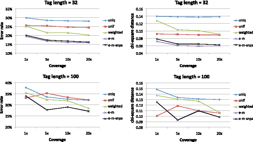
Inferring expression levels in homologous genes. In our first set of results, we compared the EM algorithms with or without SNP variant calling to previously employed methods. Figure 1 shows that both EM algorithms outperform the other methods for both 32- and 100-bp length reads as well as for the different accuracy measures. Indeed for reads of length 32 the error rate decreases from approximately 30% for the uniq method that uses only the uniquely mapped reads to approximately 20% for both EM methods. The improvement, although still substantial, is more modest for reads of length 100, probably due to a smaller number of multireads as compared to reads of length 32.
Accuracy of gene expression inference based on simulated RNA-seq data for different read lengths and different accuracy measures. Results are given as averages over 100 simulated datasets. The EM methods outperform the heuristic methods of assigning reads as well as the approach of ignoring multireads.
To further highlight the effect of including the multireads in subsequent analyses as opposed to the general approach of using only the uniquely mapped reads, we assessed the quality of SNP variant inference with or without multireads. To maintain a meaningful comparison, we called SNP variants based on unique reads under the same likelihood method for calling SNPs as in the EM algorithm of Section 2.2. Table 1 shows the true and false positive rates for SNP variant calling showing that the e–m–snps method outperforms the uniq method for all studied coverages when compared to the method that employs only the uniquely mapped reads.
Variant Calling Rates on Simulated Datasets with Reads of Length 32 for Various Coverages
Coverage
Method
TPR
FPR
1×
uniq
18.00%
2.39E-05
e-m-snps
18.26%
4.97E-05
5×
uniq
53.19%
3.27E-05
e-m-snps
55.52%
3.99E-05
10×
uniq
69.67%
4.82E-05
e-m-snps
73.55%
4.13E-05
20×
uniq
79.23%
3.50E-05
e-m-snps
83.65%
2.26E-05
Results given in averages over 100 simulated datasets.
Detecting differential expression. Using the same set of genes as before we simulated pairs of experiments with different expression levels for the genes. Using the true expression levels and a standard chi-square test (α = 0.01), we first computed a set of differentially expressed genes between the experiments which serve as the gold standard “true” differentially expressed genes. We assessed the capacity of identifying the differentially expressed genes when different methods were used for estimating
\documentclass{aastex}
\usepackage{amsbsy}
\usepackage{amsfonts}
\usepackage{amssymb}
\usepackage{bm}
\usepackage{mathrsfs}
\usepackage{pifont}
\usepackage{stmaryrd}
\usepackage{textcomp}
\usepackage{portland, xspace}
\usepackage{amsmath, amsxtra}
\pagestyle{empty}
\DeclareMathSizes {10} {9} {7} {6}
\begin{document}
$$P_i^{\prime}s$$
\end{document}. The EM method shows the overall best performance, area under ROC curve of 0.83, compared to 0.75 for the uniq method and 0.81, 0.82 for the unif and weighted methods. For α = 0.05 cutoff, EM achieves (true positive, false positive) rates of (97.5%, 24.5%)—compared to (88.4%, 20.8%) for uniq method, (95.9%,26.6%) for unif method, and (96.6%,26.4%) for weighted method.
Real dataset. We also applied our methods to a real RNA-seq data set from Marioni et al. (2008) consisting of two runs of an Illumina Genome Analyzer with half of the lanes containing human liver RNA and half kidney. We mapped all the reads with bwa (Li and Durbin, 2009) to the human genome sequence build hg18 and counted the number of reads in exons (we used the exon annotation of UCSC genome browser, http://genome.ucsc.edu/). The read counts per gene were highly correlated across lanes and did not exhibit a lane effect for most lanes (Marioni et al., 2008). We used the data from lanes one and two from the first run to estimate kidney and liver expression levels. We used the weighted method and our EM method to estimate the read counts for each gene. In this case, we do not know the true expression levels of the genes so we can not report which method is more accurate. Instead, we measure the number of genes exceeding a 5 × log2 fold change between each of the methods. The 5 log2 fold change threshold we chose has the property that all genes exceeding this threshold in both the weighted and EM methods also exceed this threshold on the Affymetrix arrays. This suggests it is so conservative that it is 100% specific with 0 false positives. It would be useful to examine specificity and sensitivity at other thresholds but the true set of differentially expressed genes (i.e., a gold standard) for making such a comparison does not exist yet, and thus we restrict ourselves to the extreme 5 log2 fold change.
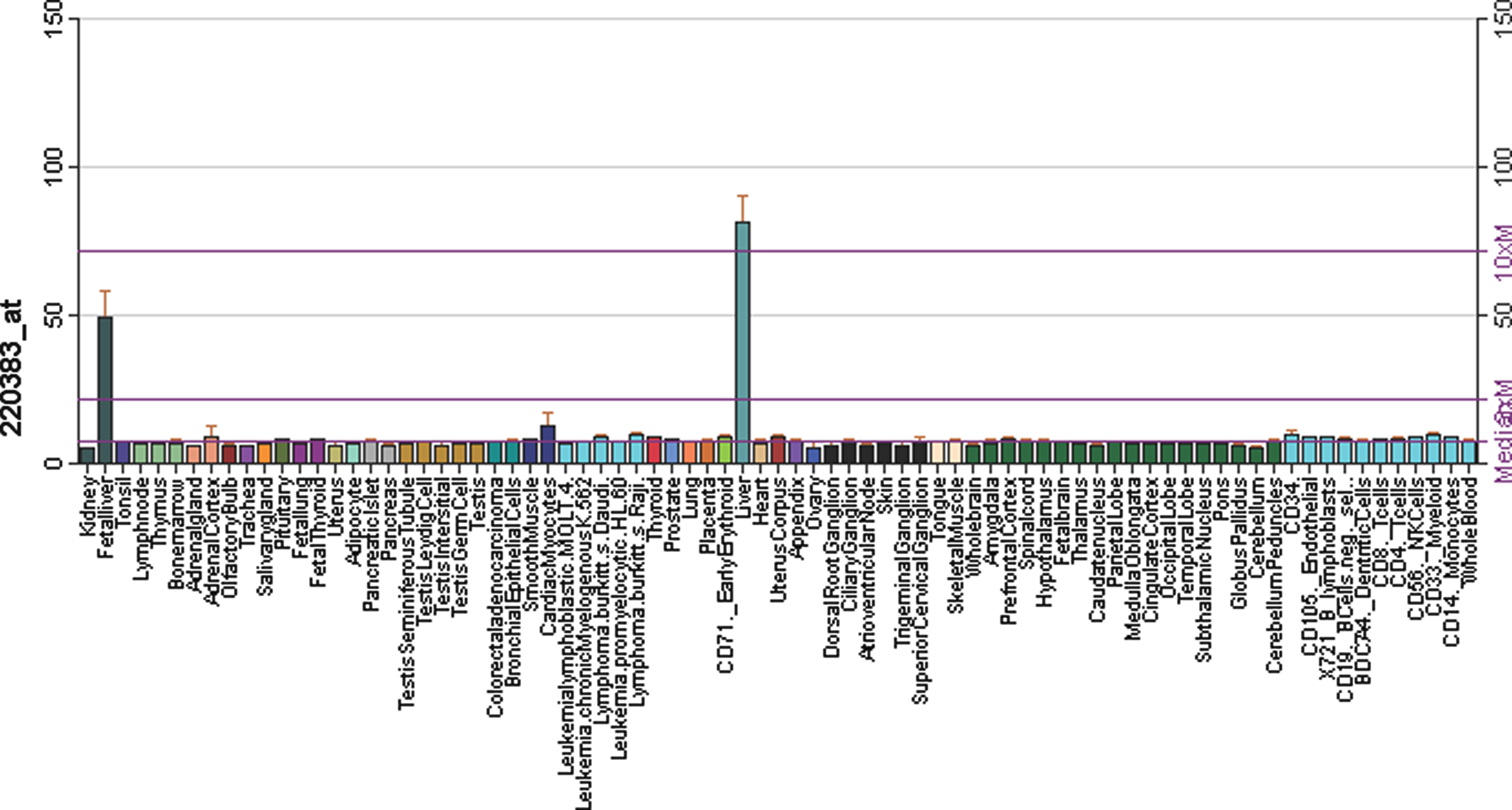
For genes with uniquely mapped reads, these methods will perform identically, so we restricted our analysis to the 2207 genes with more than 200 multireads. For this set of homologous genes, our EM method found 94 highly differentially expressed genes, while the weighted method reported only 86, a decrease of 8.5%. All of the genes found to be highly differentially expressed using the weighted method were contained in the set found using EM. To verify that the additional eight genes we found using EM were not false positives, we examined their expression levels in the GeneAtlas project (Su et al., 2004), a comprehensive survey of gene expression in human tissues. For seven of the eight additional genes, we found that GeneAtlas expression levels were consistent with the EM findings; the probe intensities were greater than 50 in one tissue and less than 10 in the other. Figure 2 shows an example for the gene ENSG00000138075 (ABCG5). Note that ABCG5 has a known homolog ABCG8, so it is one of the cases that our method addresses. Only one of these eight genes predicted to be differentially expressed by EM was not differentially expressed in the GeneAtlas. Overall, these data confirm the increased power of our method, suggesting that the additional differentially expressed genes found by the EM are true positives.
Expression levels of gene ABCG5 in the GeneAtlas (http://biogps.gnf.org) project with high expression in liver and fetal-liver. Gene ABCG5 is shown to be highly differentially expressed between liver and kidney in Marioni et al. (2008) RNA-seq data only when using our EM method for inferring gene expression levels.
4. Conclusion
Given the dropping cost of sequencing and the numerous advantages that RNA-seq has over expression array-based experiments, it is likely that in the near future RNA-seq will become a pervasive choice for measuring cellular RNA expression levels. Many of the analyses conducted so far have utilized varying methods, and it is currently unclear which strategies will prove to be the most accurate and powerful. Considering the rich literature discussing proper analysis of microarray data over the last fifteen years, it is likely that methods for this new technology can be significantly improved.
This work addresses an important aspect of RNA-seq analysis: how to handle reads from homologous and repetitive elements that map to multiple genomic locations. Our results clearly show that naive approaches significantly underestimate the true expression of homologous genes. Unlike previous heuristic approaches, we present methods based on a rigorous probabilistic generative framework for an RNA-seq experiment and show that our approach consistently outperforms all previous attempts at solving this problem. We also applied our approach on a real RNA-seq data set to find several new highly differentially expressed genes when compared to previous approaches; these findings were confirmed by existing expression array data sets.
We have identified several areas of improvement that we plan to address in future work. Currently, our method is limited to the use of consensus genes and may be improved by additionally modelling isoforms, splice variants, allelic heterogeneity, and un-annotated genes. In addition, the problem of multireads extends beyond RNA-seq experiments. For example, in both ChiP-seq and RIp-seq scenarios, array-based methods are replaced with an NGS approach, and so analysis methods must again handle multireads. Instead of determining the distribution of multireads as in RNA-seq, a binary signal is returned specifying whether or not a particular transcription factor binds to a specific genomic location. Solving the multiread problem in this context can potentially increase the power of detecting interesting loci, particularly when these loci fall within repetitive elements of the genome.
Footnotes
Acknowledgments
E.H. is a faculty fellow of the Edmond J. Safra Bioinformatics program at Tel-Aviv University. E.H. and B.P. were supported by National Science Foundation grant HS-071325412. E.H. and N.Z. were supported by the Israel Science Foundation grant no. 04514831.
Disclosure Statement
No competing financial interests exist.
References
1.
CokusS.J., FengS., ZhangX.et al.2008. Shotgun bisulphite sequencing of the Arabidopsis genome reveals DNA methylation patterning. Nature, 452:215–219.
2.
DohmJ.C., LottazC., BorodinaT.et al.2008. Substantial biases in ultra-short read data sets from high-throughput DNA sequencing. Nucleic Acids Res., 36:e105.
3.
GuttmanM., GarberM., LevinJ.Z.et al.2010. Ab initio reconstruction of cell type-specific transcriptomes in mouse reveals the conserved multi-exonic structure of lincRNAs. Nat. Biotechnol, 28:503–510.
HashimotoT., de HoonM.J., GrimmondS.M.et al.2009. Probabilistic resolution of multi-mapping reads in massively parallel sequencing data using MuMRescueLite. Bioinformatics, 25:2613–2614.
6.
JiangH., WongW.H.2009. Statistical inferences for isoform expression in RNA-Seq. Bioinformatics, 25:1026–1032.
7.
JohnsonD.S., MortazaviA., MyersR.M.et al.2007. Genome-wide mapping of in vivo protein-DNA interactions. Science, 316:1497–1502.
LiH., DurbinR.2009. Fast and accurate short read alignment with Burrows-Wheeler transform. Bioinformatics, 25:1754–1760.
10.
LiH., RuanJ., DurbinR.2008. Mapping short DNA sequencing reads and calling variants using mapping quality scores. Genome Res, 18:1851–1858.
11.
MarioniJ.C., MasonC.E., ManeS.M.et al.2008. RNA-seq: an assessment of technical reproducibility and comparison with gene expression arrays. Genome Res, 18:1509–1517.
12.
MortazaviA., WilliamsB.A., McCueK.et al.2008. Mapping and quantifying mammalian transcriptomes by RNA-Seq. Nat. Methods, 5:621–628.
13.
NicolaeM., MangulS., MandoiuI.et al.2010. Estimation of alternative splicing isoform frequencies from RNA-Seq data. Proc. WABI2687.
SuA.I., WiltshireT., BatalovS.et al.2004. A gene atlas of the mouse and human protein-encoding transcriptomes. Proc. Natl. Acad. Sci. USA, 101:6062–6067.
16.
The ENCODE Project Consortium. 2007. Identification and analysis of functional elements in 1% of the human genome by the ENCODE pilot project. Nature, 447:799–816.
17.
The International HapMap Consortium. 2007. A second generation human haplotype map of over 3.1 million SNPs. Nature, 449:851–861.
18.
TrapnellC., WilliamsB.A., PerteaG.et al.2010. Transcript assembly and quantification by RNA-Seq reveals unannotated transcripts and isoform switching during cell differentiation. Nat. Biotechnol, 28:511–515.
19.
WangZ., GersteinM., SnyderM.2009. RNA-Seq: a revolutionary tool for transcriptomics. Nat. Rev. Genet., 10:57–63.