A Blind Deconvolution Approach for Improving the Resolution of Cryo-EM Density Maps

Abstract

Cryo-electron microscopy (cryo-EM) plays an increasingly prominent role in structure elucidation of macromolecular assemblies. Advances in experimental instrumentation and computational power have spawned numerous cryo-EM studies of large biomolecular complexes resulting in the reconstruction of three-dimensional density maps at intermediate and low resolution. In this resolution range, identification and interpretation of structural elements and modeling of biomolecular structure with atomic detail becomes problematic. In this article, we present a novel algorithm that enhances the resolution of intermediate- and low-resolution density maps. Our underlying assumption is to model the low-resolution density map as a blurred and possibly noise-corrupted version of an unknown high-resolution map that we seek to recover by deconvolution. By exploiting the nonnegativity of both the high-resolution map and blur kernel, we derive multiplicative updates reminiscent of those used in nonnegative matrix factorization. Our framework allows for easy incorporation of additional prior knowledge such as smoothness and sparseness, on both the sharpened density map and the blur kernel. A probabilistic formulation enables us to derive updates for the hyperparameters; therefore, our approach has no parameter that needs adjustment. We apply the algorithm to simulated three-dimensional electron microscopic data. We show that our method provides better resolved density maps when compared with B-factor sharpening, especially in the presence of noise. Moreover, our method can use additional information provided by homologous structures, which helps to improve the resolution even further.

1. Introduction

Cryo-electron microscopy (cryo-EM) and low-resolution x-ray crystallography are emerging experimental techniques to elucidate the three-dimensional structure of large biomolecular complexes (Frank, 2002; Orlova and Saibil, 2004; Chiu et al., 2005; Brunger, 2005). A major drawback common to these methods is that the reconstructed density maps are only of intermediate or low resolution, typically in the nanometer range. In this resolution range, it becomes difficult to interpret the density maps unambiguously and to fit atomic models. A method to improve the quality of electron density maps has therefore the potential to broaden the scope of cryo-EM and low-resolution crystallography.

B-factor sharpening (DeLaBarre and Brunger, 2006; Rosenthal and Henderson, 2003; Fernández et al., 2008) is often advocated as a method for improving the resolution of density maps. The method operates in the frequency domain and applies a negative B-factor to the Fourier coefficients of the density map. This has the effect that high-frequency components encoding high-resolution features are amplified. B-factor sharpening has several limitations: First, the underlying model of the PSF is an isotropic Gaussian whose width is determined by the magnitude of the overall B-factor (the Fourier transform of a Gaussian is a Gaussian with inverted width); this assumption may be inappropriate for anisotropic data such as 2D crystals. Second, the method suffers from amplification of noise; noise in density maps contributes high-frequency components, which are weighted up when applying a negative B-factor. Third, it is not possible to incorporate prior knowledge to regularize the recovered high-resolution density map; for example, the B-factor sharpened density map is not guaranteed to be nonnegative.

In this article, we present a novel algorithm to sharpen electron density maps. The algorithm remedies some of the shortcomings of thermal factor sharpening. The underlying assumption is that low- to intermediate-resolution density maps can be viewed as distorted or “blurred” versions of high-resolution maps. Mathematically, this blurring process is modeled as a convolution \documentclass{aastex}\usepackage{amsbsy}\usepackage{amsfonts}\usepackage{amssymb}\usepackage{bm}\usepackage{mathrsfs}\usepackage{pifont}\usepackage{stmaryrd}\usepackage{textcomp}\usepackage{portland,xspace}\usepackage{amsmath,amsxtra}\pagestyle{empty}\DeclareMathSizes{10}{9}{7}{6} \begin{document} \begin{align*} y = f * x \tag{1} \end{align*} \end{document}

where y denotes the observed blurry and noisy low-resolution map, x the true high-resolution map, f the linear shift-invariant blur kernel or point spread function (PSF), and * the linear convolution operator.

We propose a blind deconvolution method (BD) to sharpen electron density maps. BD aims to invert the blurring process and thereby recover the high-resolution map without any knowledge on the degradation or blur kernel. It does so by estimating the sharpened density map and the PSF simultaneously. In this article, we are interested in BD algorithms that do not assume a particular structural model and that are in this sense parameter-free. The recovered high-resolution map will be useful for density map interpretation and model fitting.

Blind deconvolution is a severely ill-posed problem, because there exists an infinite number of solutions and small perturbations in the data lead to large distortions in the estimated true map. The ill-posedness may be alleviated by confining the set of admissible maps to those that are physically plausible through the introduction of additional constraints. One such constraint is that electron density maps are inherently nonnegative. We show that nonnegative blind deconvolution (NNBD) can be cast into a set of coupled quadratic programs that are solved using the multiplicative updates proposed in Sha et al. (2007). No learning rate has to be adjusted, and convergence of the updates is guaranteed. By iterating between an update step for x and f, we obtain an efficient BD algorithm that allows for straightforward incorporation of prior knowledge such as sparseness and smoothness of the true map and/or the PSF.

Blind deconvolution is a valuable tool in many image and signal processing applications such as computational photography, astronomy, microscopy, and medical imaging, and thus has been treated in numerous publications. Many blind deconvolution algorithms have been proposed in various fields of research (Kundur and Hatzinakos, 1996; Starck et al., 2002; Sarder and Nehorai, 2006; Levin et al., 2009). However, to our knowledge, it has never been proposed in the field of cryo-EM.

2. Blind Deconvolution by Nonnegative Quadratic Programming

Our generative model underlying the image formation process is \documentclass{aastex}\usepackage{amsbsy}\usepackage{amsfonts}\usepackage{amssymb}\usepackage{bm}\usepackage{mathrsfs}\usepackage{pifont}\usepackage{stmaryrd}\usepackage{textcomp}\usepackage{portland,xspace}\usepackage{amsmath,amsxtra}\pagestyle{empty}\DeclareMathSizes{10}{9}{7}{6} \begin{document} \begin{align*} y \approx f * x \end{align*} \end{document}

where the degraded map y, the PSF f and the true map x are n-dimensional.1 Assuming additive Gaussian noise with zero mean and variance τ⁻¹, the likelihood of observing y is given by \documentclass{aastex}\usepackage{amsbsy}\usepackage{amsfonts}\usepackage{amssymb}\usepackage{bm}\usepackage{mathrsfs}\usepackage{pifont}\usepackage{stmaryrd}\usepackage{textcomp}\usepackage{portland,xspace}\usepackage{amsmath,amsxtra}\pagestyle{empty}\DeclareMathSizes{10}{9}{7}{6} \begin{document} \begin{align*} p ( y \mid\, f , x , \tau) = Z ( \tau ) ^ { - 1 } \exp \left\{ - \frac { \tau } { 2 } \| y - f \ast x \| ^2 \right\} \end{align*} \end{document}

where ‖·‖ denotes the L₂-norm and Z the normalizing partition function, which depends only on the precision τ. As a prior, we constrain f and x to be of finite size and to lie in the nonnegative orthant: p(x) ∝ χ(x ≥ 0) and p(f) ∝ χ(f ≥ 0) where χ is the indicator function. Computation of the maximum a posteriori (MAP) estimate of f and x is equivalent to the nonnegatively constrained problem of minimizing the negative log-likelihood viewed as a function of the unknown parameters f and x: \documentclass{aastex}\usepackage{amsbsy}\usepackage{amsfonts}\usepackage{amssymb}\usepackage{bm}\usepackage{mathrsfs}\usepackage{pifont}\usepackage{stmaryrd}\usepackage{textcomp}\usepackage{portland,xspace}\usepackage{amsmath,amsxtra}\pagestyle{empty}\DeclareMathSizes{10}{9}{7}{6} \begin{document} \begin{align*} \min_ {f \,\geq\, 0 , \ x\, \geq\, 0 } L ( \,f , x ) = \frac { 1 } { 2 } \| y - f \ast x \| ^2. \tag { 2 } \end{align*} \end{document}

Here, the negative log-likelihood L is expressed in units of τ and constants independent of f and x have been dropped. Because of the interdependence of f and x through the convolution, optimization problem (2) is non-convex and a globally optimal solution cannot be found efficiently. Fortunately, the objective function L(f, x) is sufficiently well-behaved as it is convex in each variable separately if the other is held fixed. This observation suggests a simple alternating descent scheme: instead of minimizing (2) directly, we iteratively solve the minimization problems min_f ≥ 0 L(f) and min_x ≥ 0 L(x), where L(f), L(x) denotes L(f, x) for fixed f, x, respectively. If we can ensure descent in each step, we will obtain a sequence of estimates {f^(k), x^(k)} that never increase the objective L(f, x). Due to the symmetry of the convolution operation, f * x = x * f, we can restrict our exposition to the optimization of x; equivalent results will hold for f.

Because convolution is a bilinear operation, the problem of optimizing x can be written in matrix notation: \documentclass{aastex}\usepackage{amsbsy}\usepackage{amsfonts}\usepackage{amssymb}\usepackage{bm}\usepackage{mathrsfs}\usepackage{pifont}\usepackage{stmaryrd}\usepackage{textcomp}\usepackage{portland,xspace}\usepackage{amsmath,amsxtra}\pagestyle{empty}\DeclareMathSizes{10}{9}{7}{6} \begin{document} \begin{align*} \min_ { x \, \geq\, 0 } L (x ) = \frac { 1 } { 2 } \| y - f \ast x \| ^2 = \frac { 1 } { 2 } x^T F^T Fx - y^T Fx + \frac { 1 } {2} y^T y \tag { 3 } \end{align*} \end{document}

where in this formulation y, x, and f are zero-padded vectors stacked in lexicographical order and F is a block-Toeplitz structured matrix. In the following, we will use both notations interchangeably; the type of the involved quantities will be clear from the context. Minimizing (3) is equivalent to solving a quadratic program with nonnegativity constraint (NNQP) \documentclass{aastex}\usepackage{amsbsy}\usepackage{amsfonts}\usepackage{amssymb}\usepackage{bm}\usepackage{mathrsfs}\usepackage{pifont}\usepackage{stmaryrd}\usepackage{textcomp}\usepackage{portland,xspace}\usepackage{amsmath,amsxtra}\pagestyle{empty}\DeclareMathSizes{10}{9}{7}{6} \begin{document} \begin{align*} \min_ {x\, \geq \, 0 } \frac { 1 } { 2 } \, x^T A x + b^T x \tag {4} \end{align*} \end{document}

with A = F^TF and b = −F^Ty. Recently, a novel algorithm for solving NNQPs based on multiplicative updates has been proposed (Sha et al., 2007). In the derivation of the updates, only the positive semidefiniteness of A is required. In particular, A may have negative entries off-diagonal. The key idea is to decompose A into its positive and negative part, i.e., A = A⁺ − A⁻ where \documentclass{aastex}\usepackage{amsbsy}\usepackage{amsfonts}\usepackage{amssymb}\usepackage{bm}\usepackage{mathrsfs}\usepackage{pifont}\usepackage{stmaryrd}\usepackage{textcomp}\usepackage{portland, xspace}\usepackage{amsmath, amsxtra}\pagestyle{empty}\DeclareMathSizes{10}{9}{7}{6}\begin{document}$$A^{ \pm}_{ij} = ( \mid A_{ij} \mid \pm A_{ij} ) / 2$$\end{document} , and to construct an auxiliary function G(x, x′) for the objective (2) such that ∀x, x′ > 0: L(x) ≤ G(x, x′) and L(x′) = G(x′, x′). Because G(x, x′) is an upper bound on L(x), minimization with respect to x yields an estimate \documentclass{aastex}\usepackage{amsbsy}\usepackage{amsfonts}\usepackage{amssymb}\usepackage{bm}\usepackage{mathrsfs}\usepackage{pifont}\usepackage{stmaryrd}\usepackage{textcomp}\usepackage{portland, xspace}\usepackage{amsmath, amsxtra}\pagestyle{empty}\DeclareMathSizes{10}{9}{7}{6}\begin{document}$${ \hat x} = { \rm argmin}_x G ( x , x^ \prime )$$\end{document} , which never increases the objective L(x′): \documentclass{aastex}\usepackage{amsbsy}\usepackage{amsfonts}\usepackage{amssymb}\usepackage{bm}\usepackage{mathrsfs}\usepackage{pifont}\usepackage{stmaryrd}\usepackage{textcomp}\usepackage{portland,xspace}\usepackage{amsmath,amsxtra}\pagestyle{empty}\DeclareMathSizes{10}{9}{7}{6} \begin{document} \begin{align*} L ( {\hat x} ) \leq G ( { \hat x} , x^ \prime ) \leq G ( x^ \prime, x^ \prime ) \leq L ( x^ \prime). \end{align*} \end{document}

As shown in Sha et al. (2007), a valid auxiliary function for (4) is given by \documentclass{aastex}\usepackage{amsbsy}\usepackage{amsfonts}\usepackage{amssymb}\usepackage{bm}\usepackage{mathrsfs}\usepackage{pifont}\usepackage{stmaryrd}\usepackage{textcomp}\usepackage{portland,xspace}\usepackage{amsmath,amsxtra}\pagestyle{empty}\DeclareMathSizes{10}{9}{7}{6} \begin{document} \begin{align*} G (x , x^ \prime ) = \frac { 1 } { 2 } \sum_i \frac { ( A^ + x^ \prime ) _i } { x^ \prime_i } \ x_i^2 - \sum_i ( A^ - x^ \prime )_i \ x^ \prime_i \log \frac { x_i } { x^ \prime_i } + b^T x - \frac { 1 } { 2 } x^ { \prime T } A^ - x^ \prime. \tag { 5 } \end{align*} \end{document}

Minimization of (5) with respect to its first argument yields the update: \documentclass{aastex}\usepackage{amsbsy}\usepackage{amsfonts}\usepackage{amssymb}\usepackage{bm}\usepackage{mathrsfs}\usepackage{pifont}\usepackage{stmaryrd}\usepackage{textcomp}\usepackage{portland,xspace}\usepackage{amsmath,amsxtra}\pagestyle{empty}\DeclareMathSizes{10}{9}{7}{6} \begin{document} \begin{align*} x \leftarrow x \odot \frac {- b + \sqrt { b \odot b + 4 \ ( A^ + x ) \odot ( A^ - x ) } } { 2 A^ + x } . \tag { 6 } \end{align*} \end{document}

The symbol ⨀ denotes voxel-wise multiplication; also, division and square root are understood voxel-wise. For a nonnegative observed map y with A⁺ = F^TF, A⁻ = 0 and b = −F^Ty, update (6) reads \documentclass{aastex}\usepackage{amsbsy}\usepackage{amsfonts}\usepackage{amssymb}\usepackage{bm}\usepackage{mathrsfs}\usepackage{pifont}\usepackage{stmaryrd}\usepackage{textcomp}\usepackage{portland,xspace}\usepackage{amsmath,amsxtra}\pagestyle{empty}\DeclareMathSizes{10}{9}{7}{6} \begin{document} \begin{align*} x \longleftarrow x \odot \frac { F^Ty } { F^T F x } . \tag { 7 } \end{align*} \end{document}

Contrary to previous approaches to NNQP (Johnston et al., 2000), no learning rate is involved that needs adjustment. Furthermore, convergence to a global optimum is guaranteed. Note that, as f * x approaches y, the multiplicative factor in (7) tends to one. The update rules can be computed very efficiently using the Fast Fourier Transform (Press et al., 2007) because \documentclass{aastex}\usepackage{amsbsy}\usepackage{amsfonts}\usepackage{amssymb}\usepackage{bm}\usepackage{mathrsfs}\usepackage{pifont}\usepackage{stmaryrd}\usepackage{textcomp}\usepackage{portland,xspace}\usepackage{amsmath,amsxtra}\pagestyle{empty}\DeclareMathSizes{10}{9}{7}{6} \begin{document} \begin{align*} Fx \equiv f \ast x = { \cal F}^{ - 1} \{ { \cal F} ( f ) \cdot { \cal F} ( x ) \} \end{align*} \end{document}

and \documentclass{aastex}\usepackage{amsbsy}\usepackage{amsfonts}\usepackage{amssymb}\usepackage{bm}\usepackage{mathrsfs}\usepackage{pifont}\usepackage{stmaryrd}\usepackage{textcomp}\usepackage{portland,xspace}\usepackage{amsmath,amsxtra}\pagestyle{empty}\DeclareMathSizes{10}{9}{7}{6} \begin{document} \begin{align*} F^T x \equiv f \star x = {\cal F}^{ - 1} \{ { \cal F} ( f ) ^ \ast \cdot { \cal F} ( x ) \} \end{align*} \end{document}

Coming back to our original problem, namely solving (2) jointly in x and f, we propose to iterate between update steps in x and f. Cycling between (7) and (8) ensures that both f and x will remain in the nonnegative orthant. Although multiplicative updates guarantee convergence to a global optimum in the case of NNQP, the proposed NNBD scheme only ensures convergence to a stationary point. Therefore, the solution might be sensitive to the initial values of x and f. In our experiments, however, initialization was never a problem: choosing flat maps for the initial x and f always led to good results. Algorithm (1) summarizes our NNBD approach.

Algorithm 1.

Nonnegative Blind Deconvolution

Input: Degraded, blurry map y

Output: Sharp map x, blur kernel f

Initialization of f and x with positive flat maps

while

\documentclass{aastex}\usepackage{amsbsy}\usepackage{amsfonts}\usepackage{amssymb}\usepackage{bm}\usepackage{mathrsfs}\usepackage{pifont}\usepackage{stmaryrd}\usepackage{textcomp}\usepackage{portland, xspace}\usepackage{amsmath, amsxtra}\pagestyle{empty}\DeclareMathSizes{10}{9}{7}{6}\begin{document}$$\| y - f \ast x \| ^2_F > \epsilon$$\end{document}

end

return

3. Incorporation of Prior Knowledge

In the absence of noise as well as in the case of high signal-to-noise ratios2 (SNRs), our algorithm correctly decomposes a blurry observation into the true underlying map and the corresponding PSF.3 Figure 1 shows a simulated one-dimensional toy example, where x is an equispaced sample of a Gaussian mixture model and f is chosen such that it is irreducible.4 The estimated map \documentclass{aastex}\usepackage{amsbsy}\usepackage{amsfonts}\usepackage{amssymb}\usepackage{bm}\usepackage{mathrsfs}\usepackage{pifont}\usepackage{stmaryrd}\usepackage{textcomp}\usepackage{portland, xspace}\usepackage{amsmath, amsxtra}\pagestyle{empty}\DeclareMathSizes{10}{9}{7}{6}\begin{document}$${ \hat x}$$\end{document} and PSF \documentclass{aastex}\usepackage{amsbsy}\usepackage{amsfonts}\usepackage{amssymb}\usepackage{bm}\usepackage{mathrsfs}\usepackage{pifont}\usepackage{stmaryrd}\usepackage{textcomp}\usepackage{portland, xspace}\usepackage{amsmath, amsxtra}\pagestyle{empty}\DeclareMathSizes{10}{9}{7}{6}\begin{document}$${ \hat f}$$\end{document} are close to the ground truth. However, Figure 1 shows that low SNRs raise difficulties in the reconstruction process and lead to noise-fitting and unfavorable solutions.

FIG. 1.

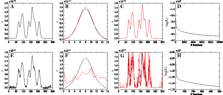
One-dimensional toy example. Top row: Results of NNBD at SNR of 60 dB. Bottom row: SNR 20 dB. (A, E) Data y used in NNBD. (B, F) True (black) and estimated (red) PSF f. (C, G) True (black), NNBD (red) estimate of the true signal x. (D, H) Negative log-likelihood (on logarithmic scale).

To further constrain the space of admissible solutions, additional knowledge about the unknown map and the PSF has to be utilized. This knowledge will be represented by non-uniform prior distributions p(f|θ) and p(x|θ) on f and x, respectively, involving hyperparameters θ. With p(θ) denoting the prior of the hyperparameters, the joint posterior is proportional to: \documentclass{aastex}\usepackage{amsbsy}\usepackage{amsfonts}\usepackage{amssymb}\usepackage{bm}\usepackage{mathrsfs}\usepackage{pifont}\usepackage{stmaryrd}\usepackage{textcomp}\usepackage{portland,xspace}\usepackage{amsmath,amsxtra}\pagestyle{empty}\DeclareMathSizes{10}{9}{7}{6} \begin{document} \begin{align*} p (x , f , \theta \mid y ) \propto p ( y \mid\, f , x , \theta ) \ p ( x \mid \theta ) \ p ( f \mid \theta ) \ p ( \theta ) . \tag{9} \end{align*} \end{document}

In the following, we describe prior distributions that are compatible with the multiplicative updates for f and x derived in the previous section. Again, because of the symmetry of (2) in f and x, we will restrict ourselves to the incorporation of prior knowledge on the unknown map x.

Incorporating priors on x introduces additional terms in (3) that have to be taken into account in the computation of the MAP estimate. In the derivation of the multiplicative update rule (6), we minimized the auxiliary function (5) defining an upper bound on L(x). A close look reveals that all priors whose negative logarithm comprises terms that are either linear, quadratic, or logarithmic in x can be incorporated into (5) and hence are compatible with the update (6). This includes the following priors:

Smoothness: A desired property in many imaging applications is smoothness of the true map, which can be enforced by penalizing the norm of its gradient ‖∇x‖. The corresponding prior is \documentclass{aastex}\usepackage{amsbsy}\usepackage{amsfonts}\usepackage{amssymb}\usepackage{bm}\usepackage{mathrsfs}\usepackage{pifont}\usepackage{stmaryrd}\usepackage{textcomp}\usepackage{portland,xspace}\usepackage{amsmath,amsxtra}\pagestyle{empty}\DeclareMathSizes{10}{9}{7}{6} \begin{document} \begin{align*} p (x \mid \lambda ) \propto \exp \left\{ - \frac { \lambda } {2} \| \nabla x \| ^2 \right\} . \tag { 10 } \end{align*} \end{document}

Note that ‖∇x‖² can be rewritten as x^TΔx where \documentclass{aastex}\usepackage{amsbsy}\usepackage{amsfonts}\usepackage{amssymb}\usepackage{bm}\usepackage{mathrsfs}\usepackage{pifont}\usepackage{stmaryrd}\usepackage{textcomp}\usepackage{portland, xspace}\usepackage{amsmath, amsxtra}\pagestyle{empty}\DeclareMathSizes{10}{9}{7}{6}\begin{document}$$\Delta x \equiv \nabla^T \nabla x = - { \cal L} \ast x$$\end{document} is the negative Laplace operator, i.e., in the one-dimensional case \documentclass{aastex}\usepackage{amsbsy}\usepackage{amsfonts}\usepackage{amssymb}\usepackage{bm}\usepackage{mathrsfs}\usepackage{pifont}\usepackage{stmaryrd}\usepackage{textcomp}\usepackage{portland, xspace}\usepackage{amsmath, amsxtra}\pagestyle{empty}\DeclareMathSizes{10}{9}{7}{6}\begin{document}$${ \cal L} = ( 1 , - 2 , 1 )$$\end{document} .

Sparseness: A further assumption commonly made is sparseness, which can be encoded in the exponential prior \documentclass{aastex}\usepackage{amsbsy}\usepackage{amsfonts}\usepackage{amssymb}\usepackage{bm}\usepackage{mathrsfs}\usepackage{pifont}\usepackage{stmaryrd}\usepackage{textcomp}\usepackage{portland,xspace}\usepackage{amsmath,amsxtra}\pagestyle{empty}\DeclareMathSizes{10}{9}{7}{6} \begin{document} \begin{align*} p (x \mid \lambda ) \propto \exp \left\{ - \lambda \sum_i \mid x_i \mid \right\} = \exp \{ - \lambda { I}^T x \} \tag{11} \end{align*} \end{document}

where the second equality holds for nonnegative maps.

Orthogonality: In some applications, it is useful to introduce a voxel-wise nonnegative background z, which results in the model y = f * x + z. Such a background could, for example, account for the solvent in electron microscopic recordings or a homologous structure for model refinement (see Section 4.1). Usually, the background should be uncorrelated with the reconstructed map, which can be enforced by penalizing the overlap between x and z, i.e. \documentclass{aastex}\usepackage{amsbsy}\usepackage{amsfonts}\usepackage{amssymb}\usepackage{bm}\usepackage{mathrsfs}\usepackage{pifont}\usepackage{stmaryrd}\usepackage{textcomp}\usepackage{portland,xspace}\usepackage{amsmath,amsxtra}\pagestyle{empty}\DeclareMathSizes{10}{9}{7}{6} \begin{document} \begin{align*} p ( x \mid \theta ) \propto \exp \{ - \lambda \ z^Tx \} . \tag{12} \end{align*} \end{document}

We treat the background as a variable that we learn along with f and x using analogous multipli-cative updates. In the following, we will refer to this regularization term as orthogonality constraint. Of course, z could be constant if such knowledge is available.

Entropy: A reasonable assumption, especially for the form of the PSF, is that it exhibits a bump-like shape. This can be favored by using the entropic prior \documentclass{aastex}\usepackage{amsbsy}\usepackage{amsfonts}\usepackage{amssymb}\usepackage{bm}\usepackage{mathrsfs}\usepackage{pifont}\usepackage{stmaryrd}\usepackage{textcomp}\usepackage{portland,xspace}\usepackage{amsmath,amsxtra}\pagestyle{empty}\DeclareMathSizes{10}{9}{7}{6} \begin{document} \begin{align*} p (x \mid \lambda ) \propto \exp \left\{ \lambda \sum_i \log x_i \right\} . \tag{13} \end{align*} \end{document}

The Burg entropy ∑_i log x_i is compliant with the auxiliary function G(x, x′) and favors maximum entropy maps, i.e., constant maps. Entropy and sparseness/orthogonality can be combined into a single prior density: a voxel-wise Gamma distribution.

Table 1 summarizes the presented prior distributions and the required modifications in (6).

Table 1.

Modifications for the Incorporation of Prior Knowledge in the Update of the True Map

Prior	A⁺	A⁻	b
Smoothness	F^TF +Δ⁺	Δ⁻	−F^Ty
Sparseness	F^TF	0	− F^T y + λI
Orthogonality	F^TF	0	−F^Ty + λz
Entropy	F^TF	λdiag{x}⁻²	−F^Ty

Δ⁺ and Δ⁻ refer to the decomposition of the negative Laplacian Δ = Δ⁺ − Δ⁻. diag{x} is a diagonal matrix with entries x_i.

3.1. Estimation of hyperparameters

An important aspect is the estimation of the unknown hyperparameters. Instead of resorting to heuristics or cross-validation, we use Bayesian inference to estimate the hyperparameters θ. For all hyperpriors introduced in the previous section, the Gamma distribution G(θ|α,β) is a conjugate prior. The ideal approach to hyperparameter estimation would be to calculate their marginal posterior distribution \documentclass{aastex}\usepackage{amsbsy}\usepackage{amsfonts}\usepackage{amssymb}\usepackage{bm}\usepackage{mathrsfs}\usepackage{pifont}\usepackage{stmaryrd}\usepackage{textcomp}\usepackage{portland,xspace}\usepackage{amsmath,amsxtra}\pagestyle{empty}\DeclareMathSizes{10}{9}{7}{6} \begin{document} \begin{align*} p (\theta \mid y ) = \int_{f \geq 0} \int_{x \geq 0} \ p ( x , f , \theta \mid y ) \ { \rm d}f \ { \rm d}x \tag{14} \end{align*} \end{document}

and determine the mean or mode (Mackay, 1996). In our case, however, exact integration over f and x is infeasible. One would have to resort to computationally intensive methods like Markov chain Monte Carlo or alternatives such as variational (Molina et al., 2006) or approximate inference (Lin and Lee, 2005). Therefore, we pursue the much simpler approach of computing the MAP estimate of the joint posterior, i.e., \documentclass{aastex}\usepackage{amsbsy}\usepackage{amsfonts}\usepackage{amssymb}\usepackage{bm}\usepackage{mathrsfs}\usepackage{pifont}\usepackage{stmaryrd}\usepackage{textcomp}\usepackage{portland,xspace}\usepackage{amsmath,amsxtra}\pagestyle{empty}\DeclareMathSizes{10}{9}{7}{6} \begin{document} \begin{align*} {\hat \theta} = {\rm argmin}_{ \theta} \ p ( { \hat f} , { \hat x}, \theta \mid y ) \tag{15} \end{align*} \end{document}

where \documentclass{aastex}\usepackage{amsbsy}\usepackage{amsfonts}\usepackage{amssymb}\usepackage{bm}\usepackage{mathrsfs}\usepackage{pifont}\usepackage{stmaryrd}\usepackage{textcomp}\usepackage{portland, xspace}\usepackage{amsmath, amsxtra}\pagestyle{empty}\DeclareMathSizes{10}{9}{7}{6}\begin{document}$${ \hat f}$$\end{document} and \documentclass{aastex}\usepackage{amsbsy}\usepackage{amsfonts}\usepackage{amssymb}\usepackage{bm}\usepackage{mathrsfs}\usepackage{pifont}\usepackage{stmaryrd}\usepackage{textcomp}\usepackage{portland, xspace}\usepackage{amsmath, amsxtra}\pagestyle{empty}\DeclareMathSizes{10}{9}{7}{6}\begin{document}$${ \hat x}$$\end{document} denote the MAP estimate of the PSF and the true map, respectively. Although it has been argued that this approximation is crude and neglects valuable information (Levin et al., 2009), the joint MAP approach led to good results in our experiments. The estimates for the hyperparameters \documentclass{aastex}\usepackage{amsbsy}\usepackage{amsfonts}\usepackage{amssymb}\usepackage{bm}\usepackage{mathrsfs}\usepackage{pifont}\usepackage{stmaryrd}\usepackage{textcomp}\usepackage{portland, xspace}\usepackage{amsmath, amsxtra}\pagestyle{empty}\DeclareMathSizes{10}{9}{7}{6}\begin{document}$${ \hat \theta}$$\end{document} can be derived by solving (15) directly. The shape parameters α and β of the Gamma hyperprior are not estimated but set to fixed values α = 1 and β close to zero. According to Jin and Zou (2009), the sensitivity of the results on the shape parameters is negligible, which was confirmed by our experiments.

3.2. Remarks

Let us come back to the one-dimensional toy example at low SNR (Fig. 1).

Figure 2A–D shows how enforcing smoothness of the signal using prior (10) prevents unfavorable noise-fitting, and effectively helps us to recover the original signal and the PSF from the blurred and noisy observation. We further investigated the estimation of the regularization parameter λ. We tested different fixed values for λ and compared the reconstruction error of and the correlation with the true signal when applying our hierachical Bayes approach. Figure 2E, F shows that the Bayes procedure yields a minimal reconstruction error and a maximal correlation for a wide range of fixed λ values. The evolution of the regularization parameter (Fig. 2G) reveals an important feature of our deconvolution algorithm. Starting at a small initial value, the regularization parameter increases rapidly within a few iterations, after which it gradually converges to a smaller optimal value. This finding may justify the heuristic regularization scheme of Shan et al. (2008), which seems to be crucial for the success of their BD algorithm on natural images (Levin et al., 2009). Shan et al. (2009) propose to start the deconvolution with a large value of λ—a conservative choice that puts higher weight on the prior than on the data. As the deconvolution improves, the regularization parameter is decreased to put more and more weight on the data. This is similar to simulated or deterministic annealing, which aims to avoid trapping in sub-optimal local minima. The advantage of our approach is that, contrary to Shan et al. (2008), we do not need to choose a schedule for adjusting λ. Rather, our update procedure automatically balances the influence of the data versus the importance of the prior.

FIG. 2.

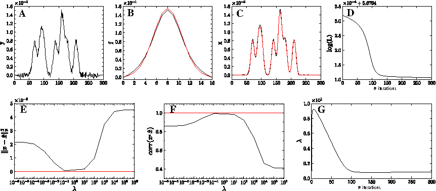
One-dimensional toy example. Top row: Results of NNBD at a SNR of 20 dB. (A) Data y used in NNBD. (B) True (black) and estimated (red) PSF f. (C) True (black), NNBD (red) estimate of the true signal x. (D) Negative log-likelihood (on logarithmic scale). Bottom row: Absolute deviation (E)/correlation coefficient (F) of the reconstructed signal \documentclass{aastex}\usepackage{amsbsy}\usepackage{amsfonts}\usepackage{amssymb}\usepackage{bm}\usepackage{mathrsfs}\usepackage{pifont}\usepackage{stmaryrd}\usepackage{textcomp}\usepackage{portland, xspace}\usepackage{amsmath, amsxtra}\pagestyle{empty}\DeclareMathSizes{10}{9}{7}{6}\begin{document}$${ \hat x}$$\end{document} from/and the true underlying signal x for fixed values of the regularization parameter λ (black) and in the case of NNBD with additional hyperparameter estimation (red) after 5000 iterations. (G) Evolution of the hyperparameter λ with increasing number of iterations.

4. Applications

To evaluate the performance of our model and verify its validity, we applied our algorithm to simulated three-dimensional density maps with a sampling of 1 Å/voxel. We used the program pdb2mrc from the EMAN software package (Ludtke et al., 1999) for density map simulation. First, we use nonnegative blind deconvolution to sharpen electron density maps. In the second application, we demonstrate the capabilities of our approach and the usefulness of the orthogonality prior by incorporating homologous structure information in the deconvolution.

4.1. Electron density maps of proteins

For validation, we used a monomer of the trimer of the bluetongue virus capsid protein VP7 (PDB ID: 2BTV) (Grimes et al., 1998). Figure 3A shows the molecular structure, Figure 3B the simulated electron density map at 10 Å resolution, and Figure 3C the corresponding PSF. Figure 3D–F shows the density map reconstructed with NNBD, the molecular structure fitted into it, and the estimated PSF. The sharpened map reveals the nature of most secondary structure elements, whereas the original density map provides ambiguous secondary structure information. Also side chains become visible, which is important for modeling atomic details. To quantify the gain in resolution, we computed the correlation coefficient between the sharpened map and density maps simulated at higher resolutions. Figure 3G shows that the correlation coefficient is highest for a density map at a resolution of 6 Å. Hence, our algorithm is able to sharpen the original map and to improve its resolution by almost a factor of two. Figure 3C,F depicts the true and estimated PSFs. The overall shape and functional form is determined correctly; however, the estimated bandwith appears to be smaller. This shrinkage of the PSF is largely due to the smoothness prior that downweights high-frequency components, which causes a loss of structural details but, at the same time, prevents amplification of noise. In this sense, underestimation of the bandwidth is conservative and should be viewed as a feature rather than a shortcoming.

FIG. 3.

NNBD for the electron density map of the monomer of the bluetongue virus outer shell coat protein VP7 (PDB ID: 2BTV). Top row: (A) Molecular structure. (B) Simulated density map at 10 Å, (C) Point spread function. Middle row: (D) NNBD reconstruction with molecular structure fitted into it. (E) NNBD reconstruction. (F) Estimated point spread function. Bottom row: (G) Correlation coefficient with simulated density maps at various resolutions. (H) Guinier plot.

Further insight is obtained by looking at the Guinier plot (Fig. 3H) showing the radially averaged power spectrum against the squared resolution. In physical terms, the Guinier plot quantifies the map's energy content at various spatial frequencies. Blurring has the effect that the Guinier plot drops off quite rapidly; convolution with a broad PSF acts as a low-pass filter that deletes all information above a certain cutoff frequency. The NNBD algorithm is able to recover high-frequency information to a large extent and lifts the Guinier curve above the curve of the simulated density map at a resolution of 6 Å (orange line in Fig. 3H).

To study the influence of noise, we corrupted the simulated density maps with Gaussian noise at different SNRs. We used the program proc3d from the EMAN software package (Ludtke et al., 1999) for noise corruption. Figure 4A shows a noisy 10 Å-density map at a SNR of 6 dB. Figure 4B shows the corresponding NNBD reconstruction using a smoothness prior (10). For comparison, Figure 4C shows the density map sharpened with embfactor (Fernández et al., 2008; Rosenthal and Henderson, 2003), the state-of-the-art method within the field.

FIG. 4.

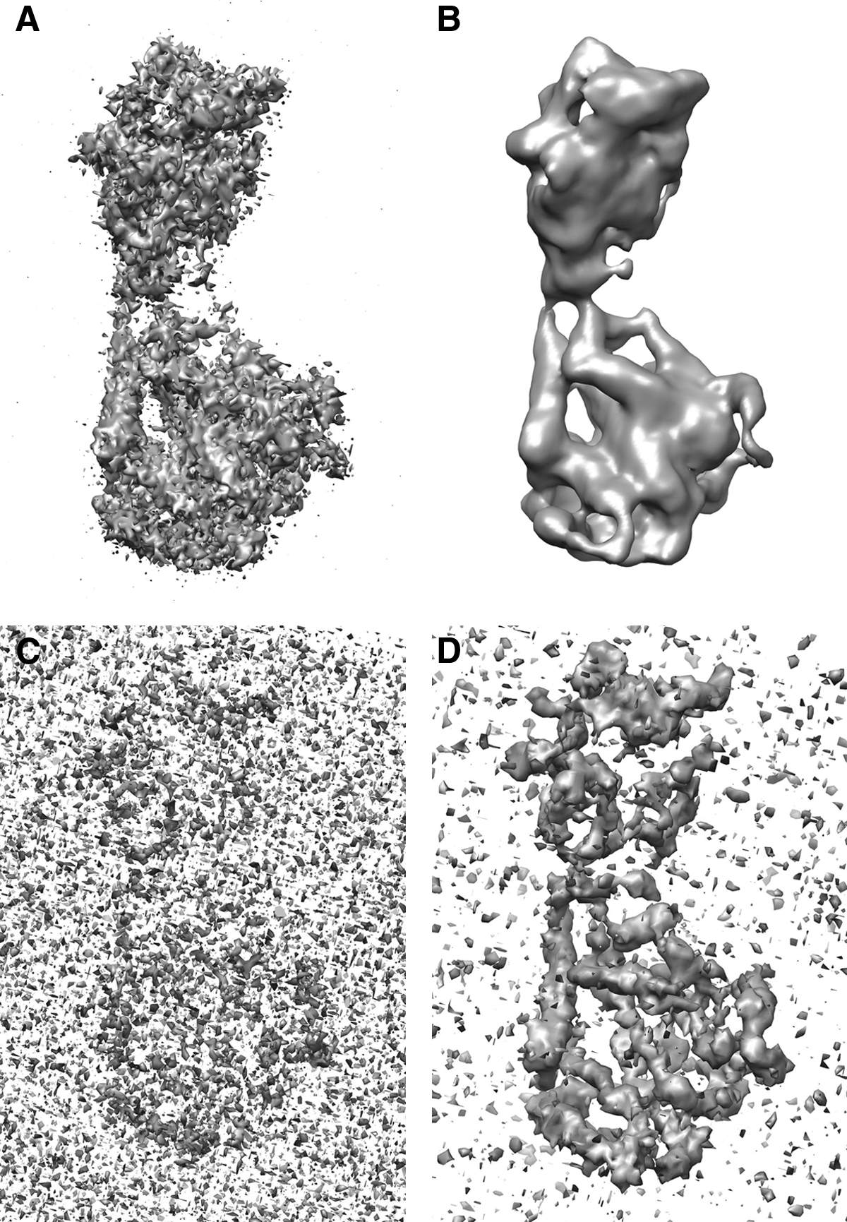
NNBD for the electron density map of the monomer of the bluetongue virus outer shell coat protein VP7 (PDB ID: 2BTV). (A) Simulated density map at SNR of 6 dB at 10 Å resolution. (B) NNBD reconstruction. (C) Result of embfactor. (D) Median-filtered result of embfactor.

4.2. Incorporating homologous structure information

We now demonstrate how additional information from homologous structures can be incorporated to aid the deconvolution process and to detect secondary structure. We use the trimeric structure of the bluetongue virus capsid protein VP7 (PDB ID: 2BTV) as an example. Figure 5A–C shows the molecular structure, and a top and side view of the simulated density of 2BTV at a resolution of 8 Å. The protein is made up of β-sheets and α-helices in the upper and lower domains, respectively. The African horse sickness virus capsid protein (PDB ID: 1AHS) is a close structural homologue (RMSD: 1.4 Å) to the all-beta domain of 2BTV. Figure 5D–F displays the molecular structure, the simulated density at a resolution of 8 Å, and the fit of 1AHS into 2BTV provided by FOLDHUNTER (Jiang et al., 2001). In B-factor sharpening, information from homologous folds is used to compute the optimal B-factor for density sharpening. In our blind deconvolution approach, we model the observed density map as being composed of the homologous structure simulated at a higher resolution and the remainder density of 2BTV. The density of the homologous fold is held fixed; only the missing density and the PSF are estimated during the deconvolution. As initial PSF, we use a Gaussian at 6 Å resolution corresponding to the resolution difference between the high-resolution density of 1AHS at 2 Å and the experimental density. During reconstruction, we apply the orthogonality constraint (12) to enforce that the 1AHS density and the unexplained region of 2BTV do not overlap. The result of NNBD is shown in Figure 5G–I. As visible in the closeup (Fig. 5I), the sharpenend density map reveals sidechains and information with almost atomic resolution. Figure 6A–C compares the true PSF and the PSFs estimated by NNBD with and without homologous structure. As in the previous example, the width of the PSF is underestimated due to the smoothness prior. However, the additional structural information facilitates a more accurate estimation of the PSF (Fig. 6C) and thereby allows the restoration of a high-resolution density map (Fig. 5I). The Guinier plot (Fig. 6D) illustrates the improved recovery of high-frequency information and the increase in resolution.

FIG. 5.

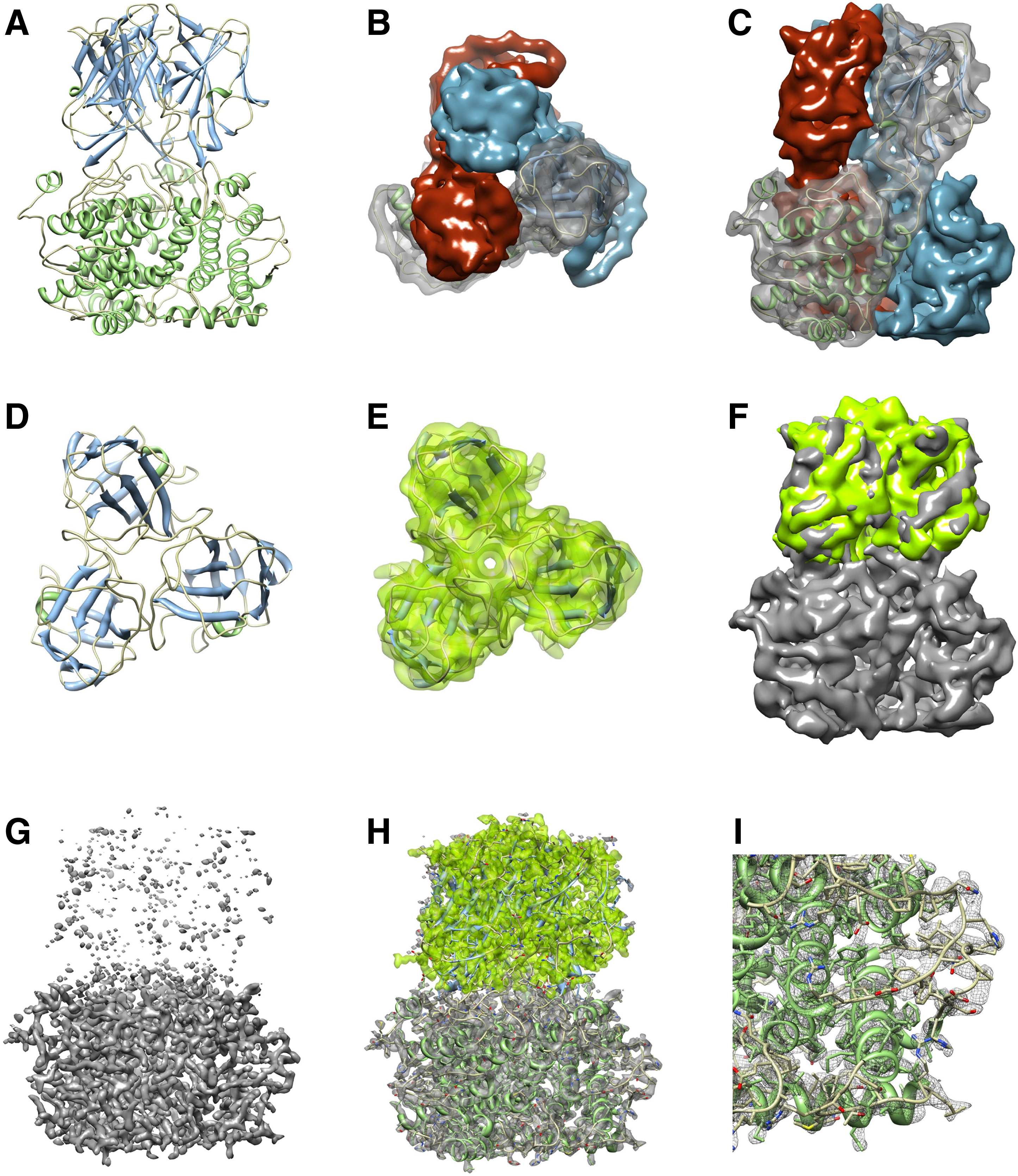
NNBD for the electron density map of the bluetongue virus capsid protein (PDB ID: 2BTV) using additional structural information from a homologous fold. Top row: (A) Molecular structure of trimer 2BTV. (B) Top view of simulated density map of 2BTV at 8 Å resolution. (C) Sideview. Middle row: (D) Molecular structure of the African horse sickness virus capsid protein (PDB ID: 1AHS). (E) Simulated density map of 1AHS at 8 Å resolution. (F) Density map of 1AHS fitted into the map of 2BTV by FOLDHUNTER. Bottom row: (G) NNBD of 2BTV without density map of homologous fold. (H) Molecular structure of 2BTV fitted into the density map. (I) Closeup view of H.

FIG. 6.

Comparison of true PSF (A), and the PSFs estimated by NNBD without (B) and with homologous structure information (C). (D) Guinier plot of reconstructed density maps with (magenta dashed line) and without homologous structure information (red dotted line).

5. Conclusion

We propose a new method for improving the resolution of cryo-EM density maps by nonnegative blind deconvolution. We provide an iterative algorithm for learning simultaneously the sharpened density map and the blur kernel. We illustrate the generality of the proposed framework and show that the derived updates allow for easy incorporation of prior knowledge such as smoothness and sparseness.The updates are multiplicative and do not require the adjustment of a learning rate, as opposed to previously proposed gradient descent techniques. In addition, the updates ensure the nonnegativity of the sharp map and the PSF and guarantee convergence to a stationary point. A hierarchical Bayesian formulation also allows us to derive update rules for the hyperparameters; thus, the method is fully parameter-free. The simplicity of the multiplicative updates allows for straightforward implementation. By employing the Fast Fourier Transform, we can reduce the computational complexity to a large extent, such that even medium and large sized problems (number of voxels > 10⁷) can be tackled efficiently. Computation time is typically on the order of minutes to hours for large-density maps (> 400³) depending on the number of iterations one is willing to perform. Since our method allows the inspection of intermediate results, the user can decide when to stop, either by visual inspection or by a user-set threshold of the monotonically decreasing cost function. We illustrate the performance and versatility of our algorithm by sharpening simulated electron density maps of the bluetongue virus capsid protein VP7 and by incorporating homologous structure information into the deconvolution process. We are currently applying our method to experimental density maps. Initial results confirm that NNDB is a flexible and generic tool to improve the resolution of electron density maps.

Footnotes

Disclosure Statement

No competing financial interests exist.

New affiliation: Max Planck Institute for Metals Research, Stuttgart, Germany.

1

The convolution is assumed to be non-circular and its value is taken only on its valid part, i.e. in the one-dimensional case, if \documentclass{aastex}\usepackage{amsbsy}\usepackage{amsfonts}\usepackage{amssymb}\usepackage{bm}\usepackage{mathrsfs}\usepackage{pifont}\usepackage{stmaryrd}\usepackage{textcomp}\usepackage{portland, xspace}\usepackage{amsmath, amsxtra}\pagestyle{empty}\DeclareMathSizes{10}{9}{7}{6}\begin{document}$$x \in {\mathbb R}^{n}$$\end{document} and \documentclass{aastex}\usepackage{amsbsy}\usepackage{amsfonts}\usepackage{amssymb}\usepackage{bm}\usepackage{mathrsfs}\usepackage{pifont}\usepackage{stmaryrd}\usepackage{textcomp}\usepackage{portland, xspace}\usepackage{amsmath, amsxtra}\pagestyle{empty}\DeclareMathSizes{10}{9}{7}{6}\begin{document}$$f \in {\mathbb R}^m$$\end{document} , then y is an element of \documentclass{aastex}\usepackage{amsbsy}\usepackage{amsfonts}\usepackage{amssymb}\usepackage{bm}\usepackage{mathrsfs}\usepackage{pifont}\usepackage{stmaryrd}\usepackage{textcomp}\usepackage{portland, xspace}\usepackage{amsmath, amsxtra}\pagestyle{empty}\DeclareMathSizes{10}{9}{7}{6}\begin{document}$${\mathbb R}^{n - m + 1}$$\end{document} . For discretized signals, * reads \documentclass{aastex}\usepackage{amsbsy}\usepackage{amsfonts}\usepackage{amssymb}\usepackage{bm}\usepackage{mathrsfs}\usepackage{pifont}\usepackage{stmaryrd}\usepackage{textcomp}\usepackage{portland, xspace}\usepackage{amsmath, amsxtra}\pagestyle{empty}\DeclareMathSizes{10}{9}{7}{6}\begin{document}$$( f \ast x ) _n = \sum\nolimits_{i \in { \rm supp} ( f ) } \ f_i x_{n - i}$$\end{document} where supp(f) denotes the support of f.

2

Here, we define the SNR of a signal as \documentclass{aastex}\usepackage{amsbsy}\usepackage{amsfonts}\usepackage{amssymb}\usepackage{bm}\usepackage{mathrsfs}\usepackage{pifont}\usepackage{stmaryrd}\usepackage{textcomp}\usepackage{portland, xspace}\usepackage{amsmath, amsxtra}\pagestyle{empty}\DeclareMathSizes{10}{9}{7}{6}\begin{document}$${\rm SNR } ( { \rm dB } ) = 10 \log_ { 10 } \frac { var ( x ) } {var ( y - x \ast f ) }$$\end{document} .

3

Note that this is true only up to an overall scaling factor, because for each estimate \documentclass{aastex}\usepackage{amsbsy}\usepackage{amsfonts}\usepackage{amssymb}\usepackage{bm}\usepackage{mathrsfs}\usepackage{pifont}\usepackage{stmaryrd}\usepackage{textcomp}\usepackage{portland, xspace}\usepackage{amsmath, amsxtra}\pagestyle{empty}\DeclareMathSizes{10}{9}{7}{6}\begin{document}$$\{ { \hat f} , { \hat x} \}$$\end{document} there exist infinitely many estimates \documentclass{aastex}\usepackage{amsbsy}\usepackage{amsfonts}\usepackage{amssymb}\usepackage{bm}\usepackage{mathrsfs}\usepackage{pifont}\usepackage{stmaryrd}\usepackage{textcomp}\usepackage{portland, xspace}\usepackage{amsmath, amsxtra}\pagestyle{empty}\DeclareMathSizes{10}{9}{7}{6}\begin{document}$$\left\{ \frac { 1 } { \lambda } { \hat f } , \lambda { \hat x } \right\}$$\end{document} with \documentclass{aastex}\usepackage{amsbsy}\usepackage{amsfonts}\usepackage{amssymb}\usepackage{bm}\usepackage{mathrsfs}\usepackage{pifont}\usepackage{stmaryrd}\usepackage{textcomp}\usepackage{portland, xspace}\usepackage{amsmath, amsxtra}\pagestyle{empty}\DeclareMathSizes{10}{9}{7}{6}\begin{document}$$\lambda \in {\mathbb R}^ +$$\end{document} that explain the observed data equally well. To rule these out, we fix the scale by normalizing f. In addition to this scale invariance, the solution is also shift-invariant. Usually this effect can be corrected only by means of further prior knowledge.

4

A signal x is irreducible, if it cannot be decomposed into two or more nontrivial components \documentclass{aastex}\usepackage{amsbsy}\usepackage{amsfonts}\usepackage{amssymb}\usepackage{bm}\usepackage{mathrsfs}\usepackage{pifont}\usepackage{stmaryrd}\usepackage{textcomp}\usepackage{portland, xspace}\usepackage{amsmath, amsxtra}\pagestyle{empty}\DeclareMathSizes{10}{9}{7}{6}\begin{document}$$\{ x_1 , x_2 , \ldots , x_n \}$$\end{document} such that \documentclass{aastex}\usepackage{amsbsy}\usepackage{amsfonts}\usepackage{amssymb}\usepackage{bm}\usepackage{mathrsfs}\usepackage{pifont}\usepackage{stmaryrd}\usepackage{textcomp}\usepackage{portland, xspace}\usepackage{amsmath, amsxtra}\pagestyle{empty}\DeclareMathSizes{10}{9}{7}{6}\begin{document}$$x = x_1 * x_2 * \ldots * x_n$$\end{document} . Note that if either f or x is reducible, NNBD becomes inherently ill-posed, because y = f * x cannot be decomposed unambiguously without employing additional prior knowledge.

References

Brunger

A.T.

2005. Low-resolution crystallography is coming of age. Structure, 13:171–172.

Chiu

, Baker

M.L.

, Jiang

et al. 2005. Electron cryomicroscopy of biological machines at subnanometer resolution. Structure, 13:363–372.

DeLaBarre

, Brunger

A.T.

2006. Considerations for the refinement of low-resolution crystal structures. Acta Crystallographica D, 62:923–932.

Fernández

J.J.

, Luque

, Castón

J.R.

et al. 2008. Sharpening high resolution information in single particle electron cryomicroscopy. J. Struct. Biol., 164:170–175.

Frank

2002. Single-particle imaging of macromolecules by cryo-electron microscopy. Annu. Rev. Biophys. Biomol. Struct., 31:303–319.

Grimes

J.M.

, Burroughs

J.N.

, Gouet

et al. 1998. The atomic structure of the bluetongue virus core. Nature, 395:470–478.

Jiang

, Baker

M.L.

, Ludtke

S.J.

et al. 2001. Bridging the information gap: computational tools for intermediate resolution structure interpretation. J. Mol. Biol., 308:1033–1044.

Jin

, Zou

2009. Augmented Tikhonov regularization. Inverse Problems, 25:025001.

Johnston

R.A.

, Connolly

T.J.

, Lane

R.G.

2000. An improved method for deconvolving a positive image. Optics Commun., 181:267–278.

10.

Kundur

, Hatzinakos

1996. Blind image deconvolution. IEEE Signal Process. Mag., 13:43–64.

11.

Levin

, Weiss

, Durand

et al. 2009. Understanding and evaluating blind deconvolution algorithms. Proc. IEEE Conf. Comput. Vision Patt. Recognit., June.

12.

Lin

, Lee

D.D.

2005. Bayesian regularization and nonnegative deconvolution for time delay estimation. Adv. NIPS, 17:809–816.

13.

Ludtke

S.J.

, Baldwin

P.R.

, Chiu

1999. EMAN: semiautomated software for high-resolution single-particle reconstructions. J. Struct. Biol., 128:82–97.

14.

MacKay

D.J.C.

1999. Hyperparameters: optimize, or integrate out? Neural Computation, 11:1035–1068.

15.

Molina

, Mateos

, Katsaggelos

A.K.

2006. Blind deconvolution using a variational approach to parameter, image, and blur estimation. IEEE Trans. Image Process., 15:3715–3727.

16.

Orlova

E.V.

, Saibil

H.R.

2004. Structure determination of macromolecular assemblies by single-particle analysis of cryo-electron micrographs. Curr. Opin. Struct. Biol., 14:584–590.

17.

Press

W.H.

, Teukolsky

S.A.

, Vetterling

W.T.

et al. 2007. Numerical Recipes: The Art of Scientific Computing, 3rd. Cambridge University Press: New York.

18.

Rosenthal

P.B.

, Henderson

2003. Optimal determination of particle orientation, absolute hand, and contrast loss in single-particle electron cryomicroscopy. J. Mol. Biol., 333:721–745.

19.

Sarder

, Nehorai

2006. Deconvolution methods for 3-D fluorescence microscopy images. IEEE Signal Process. Mag., 23:32–45.

20.

Sha

, Lin

, Saul

L.K.

et al. 2007. Multiplicative updates for nonnegative quadratic programming. Neural Comput., 19:2004–2031.

21.

Shan

, Jia

, Agarwala

2008. High-quality motion deblurring from a single image. ACM Trans. Graphics, 27:3.

22.

Starck

J.L.

, Pantin

, Murtagh

2002. Deconvolution in astronomy: a review. Publications Astronom. Soc. Pac., 114:1051–1069.